Anisotropic massive strings in scalar-tensor theory of gravitation

Abstract

We present the model of anisotropic universe with string fluid as source of matter within the framework of scalar-tensor theory of gravitation. Exact solution of field equations are obtained by applying Berman’s law of variation of Hubble’s parameter which yields a constant value of DP. The nature of classical potential is examined for the model under consideration. It has been also found that the massive strings dominate in early universe and at long last disappear from universe. This is in agreement with current astronomical observations. The physical and dynamical properties of model are also discussed.

1 Introduction

On the basis of coupling between an adequate tensor field and scalar field $\phi$, Brans and DikeBrans1961 formulated the scalar-tensor theories of gravitation. The scalar field $\phi$ has the dimension of $G^{-1}$ therefore $\phi^{-1}$ plays the role of time varying gravitational constant $G$. This theory is more consistent with Mach’s principle and less reliant on the absolute properties of space. A detail survey of Brans-Dike theory has been done by Singh and RaiSingh1983 . In fact the notion of time-dependent $G$ was first conceived by DiracDirac1938 , though Dirac’s arguments were based on cosmological considerations not directly concerned with Mach’s principle.

In Brans-Dike theory, which is the generalisation of general relativity, an additional scalar field $\phi$ besides the metric tensor $g_{ij}$ and a dimensionless coupling constant $\omega$ were introduced. For large value of coupling constant $\omega$ (i. e. $\omega>500$), Brans-Dike theory follows the result of general relativity. Later on, Saez and BallesterSaez1985 developed a scalar-tensor theory in which a dimensionless scalar field is coupled with metric. This coupling use to give a satisfactory description of the weak fields. This scalar-tensor theory play an important role to solve the missing matter problem and to remove the graceful exit problem in non flat FRW cosmologies and inflation eraPiemental1997 respectively. The following authors, Singh and AgarwalSingh1991 ; Singh1992 , Reddy et alReddy2006 ; Reddy2008 , Socorro and SabiboSocorro2010 and recently Jamil et alJamil2012 have studied cosmological model within the framework of Sa’ez-Ballester scalar-tensor theory of gravitation in different physical contexts.

Among the different cosmological structure of universe, the cosmic string models have wide acceptance because it give rise to density perturbations which lead to formation of galaxiesVilenkin1985 . Firstly, LetelierLatelier1979 described the gravitational effect of massive strings which are formed by geometric strings with particles attached along their extension. At the observational front, Pogasian et alPogosian2003 have showed that the cosmic strings are not responsible for either the CMB fluctuations or the observed clustering of galaxies. Recently Yadav et alYadav2011 and YadavYadav2012 have studied Bianchi-V string cosmological models in general relativity. In this paper, we discuss Einstein’s field equations in scalar tensor theory of gravitation for Bianchi - V space-time, filled with string fluid as source of matter. Exact solution of field equations are obtained by applying the law of variation of Hubble’s parameter, firstly proposed by BermanBerman1983 . This law yield the constant value of DP.

2 Matric and Basic equations

The spatially homogeneous and anisotropic Bianchi-V space-time is described by the line element

$$ds^{2}=-dt^{2}+A^{2}dx^{2}+e^{2\alpha x}\left(B^{2}dy^{2}+C^{2}dz^{2}\right)$$ (1)

where $A(t)$, $B(t)$ and $C(t)$ are the scale factors in different spatial directions and $\alpha$ is a constant.
We define the average scale factor $(a)$ of Bianchi-type V model as

$$a=(ABC)^{\frac{1}{3}}$$ (2)

The spatial volume is given by

$$V=a^{3}=ABC$$ (3)

Therefore, the mean Hubble’s parameter $(H)$ read as

$$H=\frac{\dot{a}}{a}=\frac{1}{3}\left(H_{1}+H_{2}+H_{3}\right)$$ (4)

where $H_{1}=\frac{\dot{A}}{A}$, $H_{2}=\frac{\dot{B}}{B}$ and $H_{3}=\frac{\dot{C}}{C}$ are the directional Hubble’s parameters in the direction of $x$, $y$ and $z$ respectively. An over dot denotes differentiation with respect to cosmic time t.

We define the kinematical quantities such as expansion scalar $(\theta)$, shear scalar $(\sigma)$ and anisotropy parameter $(A_{m})$ as follows:

$$\theta=u;^{i}_{i}$$ (5)

$$\sigma^{2}=\frac{1}{2}\sigma_{ij}\sigma^{ij}$$ (6)

$$A_{m}=\frac{1}{3}\sum_{i=1}^{3}\left(\frac{H_{i}-H}{H}\right)^{2}$$ (7)

where $u^{i}=(0,0,0,1)$ is a matter four velocity vector and

$$\sigma_{ij}=\frac{1}{2}\left(u_{i;\alpha}P^{\alpha}+u_{j;\alpha}P^{\alpha}_{i}\right)-\frac{1}{3}\theta P_{ij}$$ (8)

Here, the projection vector $P_{ij}$ has the form

$$P_{ij}=g_{ij}-u_{i}u_{j}$$ (9)

The expansion scalar $(\theta)$ and shear scalar $(\sigma)$, in Bianchi-V space-time, have the form

$$\theta=3H=\frac{\dot{A}}{A}+\frac{\dot{B}}{B}+\frac{\dot{C}}{C}$$ (10)

$$2\sigma^{2}=\left[\left(\frac{\dot{A}}{A}\right)^{2}+\left(\frac{\dot{B}}{B}\right)^{2}+\left(\frac{C}{C}\right)^{2}\right]-\frac{\theta^{2}}{3}$$ (11)

Here, $(;)$ stands for covariant derivative with respect to cosmic time $t$.

3 Field equations

We consider homogeneous and anisotropic Bianchi-V metric coupled with scalar field $\phi$. Our model is based on Saez-Ballester theory of gravitation which is based on coupling of dimensionless scalar field with metric.

We assume the Lagrangian

$$L=R-\omega\phi^{r}\phi_{,i}\phi^{,i}$$ (12)

where $R$, $\omega$ and $r$ represent the scalar curvature, coupling constant and dimensionless arbitrary constant respectively.
For the scalar field having the dimensions of $G^{-1}$, the Lagrangian (12) is not physically admissible because two terms of the right hand side of equation (12) have different dimension. However, it is suitable Lagrangian in the case of dimensionless scalar field.
From the above Lagrangian, we can establish the action

$$I=\int_{\Sigma}(L+8\pi L_{m})(-g)^{\frac{1}{2}}dx^{1}dx^{2}dx^{3}dx^{4}$$ (13)

where $L_{m}$ is the matter Lagrangian, $g$ is the determinant of the matrix $g_{ij}$, $x^{i}$ are the coordinates and $\Sigma$ is an arbitrary region of integration.
The variational principle $\delta I=0$ leads to the field equations

$$G_{ij}-\omega\phi^{r}\left(\phi_{,i}\phi_{,j}-\frac{1}{2}g_{ij}\phi_{,\ell}\phi^{,\phi}\right)=-8\pi T_{ij},$$

$$2\phi^{r}\phi^{,i}_{;i}+r\phi^{r-1}\phi_{,\ell}\phi^{,\ell}=0$$ (14)

Equation (14) is obtained by considering arbitrary independent variations of the metric and scalar field vanishing at the boundary of $\Sigma$.

Since, the action $I$ is a scalar, it can easily proved that the equation of motion

$$T^{ij}_{;i}=0$$ (15)

are consequences of the field equations.
The energy momentum tensor for a cloud of massive strings and perfect fluid distribution is taken as

$$T_{ij}=(\rho+p)u_{i}u_{j}+pg_{ij}-\lambda x_{i}x_{j}$$ (16)

where $p$ is isotropic pressure; $\rho$ is the proper energy density for the cloud of strings with particle attached to them; $\lambda$ is the string tension density; $x^{i}$ is a unit space-like vector representing the direction of string.

Choosing $x^{i}$ parallel to $\frac{\partial}{\partial x}$, we have

$$x^{i}=(A^{-1},0,0,0)$$ (17)

Here, the cosmic string has been directed along x-axis.

If the particle density of the configuration is denoted by $\rho_{p}$, then

$$\rho=\rho_{p}+\lambda$$ (18)

The Einstein’s field equations (in gravitational units $c=1$, $8\pi G=1$)

$$R_{ij}-\frac{1}{2}Rg_{ij}=-T_{ij}$$ (19)

The Einstein’s field equations (19) for the line-element (1) lead to the following system of equations

$$\frac{\ddot{B}}{B}+\frac{\ddot{C}}{C}+\frac{\dot{B}\dot{C}}{BC}-\frac{\alpha^{2}}{A^{2}}=-p+\frac{1}{2}\omega\phi^{r}{\dot{\phi}}^{2}+\lambda$$ (20)

$$\frac{\ddot{A}}{A}+\frac{\ddot{C}}{C}+\frac{\dot{A}\dot{C}}{AC}-\frac{\alpha^{2}}{A^{2}}=-p+\frac{1}{2}\omega\phi^{r}{\dot{\phi}}^{2}$$ (21)

$$\frac{\ddot{A}}{A}+\frac{\ddot{B}}{B}+\frac{\dot{A}\dot{B}}{AB}-\frac{\alpha^{2}}{A^{2}}=-p+\frac{1}{2}\omega\phi^{r}{\dot{\phi}}^{2}$$ (22)

$$\frac{\dot{A}\dot{B}}{AB}+\frac{\dot{A}\dot{C}}{AC}+\frac{\dot{B}\dot{C}}{BC}-\frac{3\alpha^{2}}{A^{2}}=\rho-\frac{1}{2}\omega\phi^{r}{\dot{\phi}}^{2}$$ (23)

$$\frac{2\dot{A}}{A}-\frac{\dot{B}}{B}-\frac{\dot{C}}{C}=0$$ (24)

$$\ddot{\phi}+\left(\frac{\dot{A}}{A}+\frac{\dot{B}}{B}+\frac{\dot{C}}{C}\right)+\frac{r}{2\phi}{\dot{\phi}}^{2}=0$$ (25)

The energy conservation equation $T^{ij}_{;j}=0$ yields

$$\dot{\rho}+3(\rho+p)H-\lambda\frac{\dot{A}}{A}=0$$ (26)

4 Solution of the field equations

We have a system of six equations (20)$-$(26) involving seven unknown variables namely, $A$, $B$, $C$, $p$, $\rho$, $\lambda$ and $\phi$. Therefore, in order to solve the field equations completely, we need at least one suitable physical assumption among the unknown variables. So, we constrain the system of equations with the law of variation for the Hubble’s parameter proposed by BermanBerman1983 , which yields a constant value of DP. This law reads as

$$H=Da^{-n}$$ (27)

where $D$ and $n$ are positive constants. In this paper, we show how the constant DP models with metric (1) behave in the presence of string fluid and dimensionless scalar field $\phi$.
The deceleration parameter $(q)$, an important observational quantity, is defined as

$$q=-\frac{a\ddot{a}}{{\dot{a}}^{2}}$$ (28)

From equations (4) and (27), we get

$$\dot{a}=Da^{-n+1}$$ (29)

Integration of (29) leads to

$$a=(nDt+c_{1})^{\frac{1}{n}},\;\;\;\;\;(n\neq 0)$$ (30)

It is important to note here that for $n=0$, the model has non singular origin and it evolves with exponential expansion which seems reasonable to project the dynamics of future Universe. Since we are looking for a model of Universe, which describe the dynamics of Universe from big bang to present epoch. Hence in this paper, the case $n=0$ has been omitted.

Integrating equation (24) and absorbing the constant of integration in $B$ or $C$, without loss of generality, we obtain

$$A^{2}=BC$$ (31)

Subtracting equation (21) from equation (22) and taking second integral, we get the following relation

$$\frac{B}{C}=d_{1}exp\left[x_{1}\int{\frac{dt}{V}}\right]$$ (32)

where $d_{1}$ and $x_{1}$ are constants of integration.

From equations (3), (30), (31) and (32), the metric function can be explicitly written as

$$A=(nDt+c_{1})^{\frac{1}{n}}$$ (33)

$$B=\sqrt{d_{1}}(nDt+c_{1})^{\frac{1}{n}}exp\left[\frac{x_{1}}{2D(n-3)}(nDt+c_{1})^{\frac{n-3}{3}}\right]$$ (34)

$$C=\frac{1}{\sqrt{d_{1}}}(nDt+c_{1})^{\frac{1}{n}}exp\left[-\frac{x_{1}}{2D(n-3)}(nDt+c_{1})^{\frac{n-3}{3}}\right]$$ (35)

provided that $n\neq 3$.

Inserting equation (4) into equation (25) and then integrating, we obtain

$$\dot{\phi}^{2}\phi^{r}=d_{2}a^{-6}$$ (36)

Here, $d_{2}$ is constant of integration.

The average’s Hubble’s parameter $(H)$, isotropic pressure $(p)$, proper energy density $(\rho)$, string tension density $(\lambda)$ and particle energy density $(\rho_{p})$ are found to be

$$H=\frac{D}{nDt+c_{1}}$$ (37)

$$p=\alpha^{2}(nDt+c_{1})^{-\frac{2}{n}}-\left(\frac{2\omega d_{2}-x_{1}^{2}}{4}\right)(nDt+c_{1})^{-\frac{6}{n}}-3(1-n)D^{2}(nDt+c_{1})^{-2}$$ (38)

$$\rho=3D^{2}(nDt+c_{1})^{-2}-\frac{(x_{1}^{2}+2\omega d_{2})}{4}(nDt+c_{1})^{-\frac{6}{n}}-3\alpha^{2}(nDt+c_{1})^{-\frac{2}{n}}$$ (39)

$$\lambda=\frac{(x_{1}^{2}-\omega d_{2})}{4}(nDt+c_{1})^{-\frac{6}{n}}$$ (40)

$$\rho_{p}=3D^{2}(nDt+c_{1})^{-2}-\frac{3x_{1}^{2}}{4}(nDt+c_{1})^{-\frac{6}{n}}-3\alpha^{2}(nDt+c_{1})^{-\frac{2}{n}}$$ (41)

The above solutions satisfy the energy conservation equation (26) identically, as expected.

The spatial volume $(V)$, expansion scalar $(\theta)$ and DP (q) are given by

$$V=(nDt+c_{1})^{\frac{3}{n}}$$ (42)

$$\theta=3D(nDt+c_{1})^{-1}$$ (43)

$$q=n-1$$ (44)

We observe that at $t=-\frac{c_{1}}{nD}$, the spatial volume vanishes while all other parameters diverge. Therefore, the model has a big bang singularity at $t=-\frac{c_{1}}{nD}$. This singularity is point type because the directional scale factors $A(t)$, $B(t)$ and $C(t)$ vanish at the initial moment. From equation (43), it is clear that for $n=1$, the universe expands with constant rate. However, the recent observations of SN Ia (Perlmutter et alPerlmutter1997 $-$Perlmutter1999 Riess et alRiess1998 ; Riess2004 and Tonry et alTonry2003 ) reveal that the present Universe is accelerating and value of DP lies somewhere in the range $-1<q<0$. It follows that one can choose the value of $n$ in the range $0<n<1$ to have the consistancy of derived model with observations.

In the derived model, the scale factors increase with time. But the contribution of exponential terms to the scale factors $B$ and $C$ becomes negligible for sufficiently large time i. e. for sufficiently large time we have $A(t)\approx B(t)\approx C(t)$. This may be observed from equation (33)$-$(35). Thus, initially the growth of scale factors take place at different rates due to effective contribution of exponential terms in $B$ and $C$. But later on the scale factors grow at the same rate. Therefore, in the derived model, the early anisotropic Universe becomes isotropic at later times.

The scalar function $(\phi)$ may be obtained as

$$\phi=\left[\frac{\phi_{0}(r+2)}{2D(n-3)}(nDt+c_{1})^{\frac{n-3}{n}}\right]^{\frac{2}{r+2}}$$ (45)

where $\phi_{0}$ is the constant of integration.

The shear scalar $(\sigma)$ and anisotropy parameter $(A_{m})$ are read as

$$\sigma=\frac{x_{1}}{2}(nDt+c_{1})^{-\frac{3}{n}}$$ (46)

$$A_{m}=\frac{x_{1}^{2}}{6D^{2}}(nDt+c_{1})^{\frac{2n-6}{n}}$$ (47)

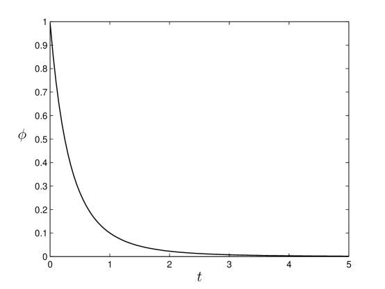
Figure 1: Plot of scalar function $(\phi)$ vs. time.

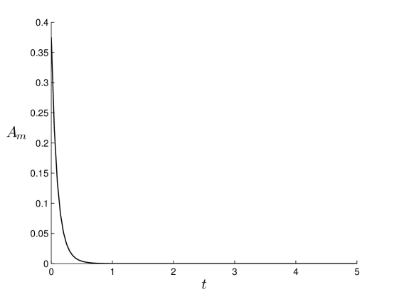
Figure 2: Plot of anisotropy parameter $(A_{m})$ vs. time

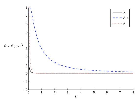
Figure 3: Plot of proper energy density $(\rho)$, string tension density $(\lambda)$ and particle energy density $(\rho_{p})$ vs. time.

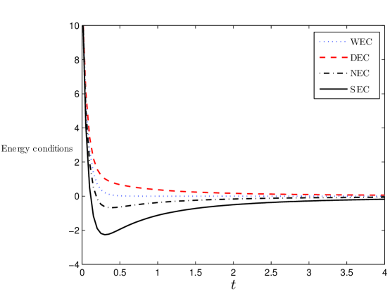
Figure 4: The left hand side of energy conditions vs. time.

The behaviours of $\rho$, $\rho_{p}$ and $\lambda$ are depicted in Figure 3. From eq. (40) and (41), it is clear that for $n<1$ and for large value of time, $\frac{\rho_{p}}{\lambda}>1$. This means that the particles dominate the strings at later times which confirms the disappearance of strings in the present day observations.

The behaviour of scalar function $(\phi)$ is depicted in figure 1. From equation (47), it is clear that for $n<1$, the anisotropy parameter $(A_{m})$ vanishes at late time. The behaviour of $A_{m}$ versus time is shown in figure 2.

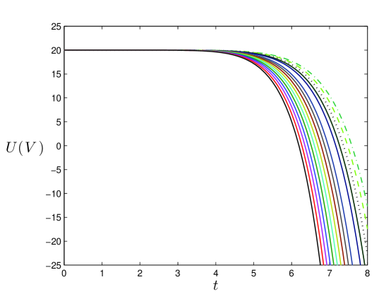
Figure 5: The classical potential vs. time.

From equation (42), we obtain

$$\dot{V}=3D(nDt+c_{1})^{\frac{3-n}{n}}$$ (48)

According to Saha and Boyadjiev Saha2004 , the equation of motion of a single particle with unit mass under force F(V) can be described as

$$\dot{V}=\sqrt{2[\in-U(V)]}$$ (49)

where $U(V)$ and $\in$ are the classical potential of force F and viewed energy level respectively.
From equations (48) and (49), we obtain

$$U(V)=2\in-9D^{2}(nDt+c_{1})^{\frac{6-2n}{n}}$$ (50)

In connection, with Hubble’s parameter the classical potential $(U)$ is given by

$$U(V)=2\in-9D^{\frac{6}{n}}H^{\frac{2n-6}{n}}$$ (51)

Figure 4 plots the left hand side of energy conditions versus time. We observe that the weak energy condition (WEC) and dominant energy condition (DEC) are satisfied in the derived model. The null energy condition (NEC) is violated in the early universe but it is eventually satisfied in the present universe. It can also be observed that the strong energy condition (SEC) is violated in the derived model. The violation of SEC gives a reverse gravitation effect which may be possible cause for late time accelerated expansion of universe. Figure 5 plots the classical potential with respect to time in presence of string fluid as source of matter. We observe that $U(V)$ shows positive and negative nature with respect to time.

5 Conclusion

In this paper, we have studied Bianchi - V string cosmological model in scalar - tensor theory of gravitation. The study reveals that the sting tension density $(\lambda)$ vanishes at present epoch that is why strings disappears from present universe but it was playing a significant role in the expansion of early universe. The derived model is singular in nature and it has big bang singularity at $t=-\frac{c_{1}}{nD}$. Thus the universe starts evolving from the infinite big bang singularity at $t=-\frac{c_{1}}{nD}$ and expands with power law expansion rate. The spatial volume is zero at initial moment $t=-\frac{c_{1}}{nD}$. At this instant, the physical parameters $\rho$, $p$, $\lambda$, $\rho_{p}$, $H$ and $\sigma$ all assume infinite values. These parameters are decreasing function of time and ultimately tend to zero for sufficiently large value of time. The spatial volume tends to zero as $t\rightarrow\infty$. Thus, the universe is essentially an empty space-time for large t.

The age of universe is given by

$$T=\frac{1}{(q+1)}H^{-1}-\frac{c_{1}}{(q+1)D}$$

Thus the age of universe increases with $-1<q<0$ which shows the consistency of derived model with observations.

We have also discussed the classical potential with respect to time and have observed that the classical potential changes its nature with evolution of universe. In early universe, it is found positive and grows with constant rate but at late time, it is ruled with negative value and decreases rapidly with time.

References

- (1) Brans C., Dike, R.: Phys. Rev., 124, 925, (1961)
- (2) Singh, T., Rai, L. N.: Gen. Relativ. Grav., 15, 875, (1983)
- (3) Dirac, P. A. M.: Proc. Roy. Soc. London, A165, 199, (1938)
- (4) Saez, D., Ballester, V. J.: Phys. Lett. A, 113, 467 (1985)
- (5) Piemental, L. O.: Mod. Phys. Lett. A, 12, 1865 (1997)
- (6) Singh, T., Agarwal, A. K.: Astrophys. Space Sc., 182, 289 (1991)
- (7) Singh, T., Agarwal, A. K.: Astrophys. Space Sc., 191, 61 (1992)
- (8) Reddy, D. R. K., Naidu, R. L., Rao, V. U. M.: Astrophys. Space Sc., 306, 185, (2006)
- (9) Reddy, D. R. K., Govinda, P., Naidu, R. L.: Int. J. Theor. Phys., 47, 2966, (2008)
- (10) Socorro, J., Sabido, M.: Revista Mexicana De Fisica, 56, 166 (2010)
- (11) Jamil, M., Ali, S., Momeni, D.: Eur. Phys. J. C, 72, 1998 (2012)
- (12) Vilenkin, A.: Phys. Rep., 121, 263, (1985)
- (13) Latelier, P. S.: Phys. Rev. D, 20, 1294, (1979)
- (14) Pogosian, L., Tye, S. H., Wasserman, I. and Wyman. M.: Phys. Rev. D, 68, 023506, (2003)
- (15) Yadav, A. K., Yadav, V. K. and Yadav, L.: Pramana J. Phys., 76, 681, (2011)
- (16) Yadav, A. K.: Research in Astron. Astrophys., 12, 1467 (2012)
- (17) Berman, M. S.: Nuovo Cimento B, 74, 182, (1983)
- (18) Perlmutter, S., et al: Astrophys. J., 483, 565 (1997)
- (19) Perlmutter, S., et al: Nature, 391, 51, (1998)
- (20) Perlmutter, S., et al: Astrophys. J., 517, 565 (1999)
- (21) Riess, R. G., et al: Astron J., 116, 1009, (1998)
- (22) Riess, R. G., et al: Astrophys. J., 607, 665 (2004)
- (23) Tonry, J. L., et al: Astrophys. J., 594, 1, (2003)
- (24) Saha, B., Boyadjiev, T.: Phys. Rev. D, 69, 124010, (2004)