Abstract

An initial-boundary value problem for the 1D self-adjoint parabolic equation on the half-axis is solved. We study a broad family of two-level finite-difference schemes with two parameters related to averagings both in time and space. Stability in two norms is proved by the energy method. Also discrete transparent boundary conditions are rigorously derived for schemes by applying the method of reproducing functions. Results of numerical experiments are included as well.

MSC classification: 65M06, 65M12

Keywords: parabolic equations, unbounded domains, finite-difference schemes, stability, discrete transparent boundary conditions

1 Introduction

In many applications, a problem of solving partial differential equations in unbounded domains arises. A number of approaches to the problem is developed mainly associated with the statement of additional boundary conditions on artificial boundaries [1]-[6]. The conditions are called the (exact) artificial/non-reflecting/transparent boundary conditions provided that they are satisfied by the solutions of the original problems in unbounded domains. For definiteness, we exploit the last name (TBCs). For parabolic evolution equations or for the Schroödinger equation, the TBCs are integro-differential relations along the artificial boundaries. Their adequate discretization is non-trivial since it can produce significant reflections from the boundaries and even instability in computations as well as create difficulties in rigorous proofs of stability of the resulting numerical method.

An alternative approach suggests to implement the idea of the TBCs on the mesh level. Namely, first one consider a discretization of the problem on an infinite mesh in the unbounded domain (which is not practical because of the infinite number of unknowns). Its solution is restricted to the finite mesh by deriving a mesh counterpart of the TBC on the artificial boundary. One version of this approach is associated with the derivation of discrete TBCs requiring to solve analytically model mesh problems on infinite grids. This approach had worked well by the complete absence of reflections from artificial boundaries and reliable stability of computations in practice as well as by clarity of the mathematical background and rigorous proofs of stability of the resulting mesh method in theory. Such an approach is developed in detail for 1D time-dependent Schrödinger equation in [7]-[11] and also used for 1D parabolic equations in [1, 12, 8, 6, 13].

In this paper, the approach is developed for the 1D self-adjoint parabolic equation on the half-axis. We study a broad family of two-level finite-difference $\sigma$-schemes with averaging in space with a weight $\theta$. We prove its stability by the energy method and rigorously derive the discrete TBC by applying the method of reproducing functions. Notice that both points are not so well developed in some other papers. Similarly to [11], this allows one to cover in a unified manner a collection of particular schemes: the standard scheme without averaging ($\theta=0$), the linear finite-element method ($\theta=\frac{1}{6}$), scheme of higher order of accuracy (for constant coefficients, $\theta=\frac{1}{12}$) and a vector scheme on a four-point stencil ($\theta=\frac{1}{4}$). The results generalize those obtained for $\theta=0$ in [13] but here we prove stability in two (not one) energy norms, the rigorous derivation of the discrete TBC is notably different and results of numerical experiments are included as well.

Notice that the results for the family of finite-difference schemes can be enlarged for the 2D (or multi-D) case exploiting the technique from [14, 15].

2 An initial-boundary value problem and a finite-difference $\sigma$-scheme with averaging in space and an approximate TBC

We consider the one-dimensional parabolic equation

$$\rho\,\frac{\partial u}{\partial t}+{\mathcal{A}}u=f,\ \ {\mathcal{A}}u:=-\frac{\partial}{\partial x}\left(b\frac{\partial u}{\partial x}\right)+cu$$ (1)

for $x>0$ and $t>0$. Its coefficients satisfy the conditions $\rho(x)\geqslant\underline{\rho}>0$, $b(x)\geqslant\nu>0$ and $c(x)\geqslant 0$ for $x>0$.

Equation (1) is supplemented with the following boundary condition, the condition at infinity and the initial condition:

$$u|_{x=0}=g(t),\ \ u(x,t)\to 0\ \ \mbox{as}\ x\to\infty,\ \mbox{for all}\ t>0,$$ (2)

$$\left.u\right|_{t=0}=u^{0}(x)\ \ \mbox{for}\ x>0.$$ (3)

We assume that the coefficients become constants as well as $f$ and $u^{0}$ vanish for sufficiently large $x\geqslant X_{0}$ (for some $X_{0}>0$)

$$\rho(x)=\rho_{\infty}>0,\ b(x)=b_{\infty}>0,\ c(x)=c_{\infty}\geqslant 0,\ f(x,t)=0,\ u^{0}(x)=0.$$ (4)

An integro-differential TBC satisfied by the solution to this problem can be written in the Dirichlet-to-Neumann form

$$\frac{\partial u}{\partial x}\,(X,t)=-\sqrt{\frac{\rho_{\infty}}{b_{\infty}}}\,e^{\displaystyle{-(c_{\infty}/\rho_{\infty})t}}\,\frac{1}{\sqrt{\pi}}\frac{d}{dt}\int_{0}^{t}u(X,\theta)e^{\displaystyle{(c_{\infty}/\rho_{\infty})\theta}}\,\frac{d\theta}{\sqrt{t-\theta}}$$ (5)

for $t>0$ and for any $X\geqslant X_{0}$; other equivalent forms are also known. The TBC is nonlocal in time; recall that the involved operator

$$\mathcal{D}_{t+}^{1/2}w(t):=\frac{1}{\sqrt{\pi}}\frac{d}{dt}\int_{0}^{t}w(\theta)\,\frac{d\theta}{\sqrt{t-\theta}}\ \ \mbox{for}\ \ t>0$$

defines the classical left-hand Riemann-Liouville time derivative of order $\frac{1}{2}$ on the half-axis $[0,\infty)$. But we do not exploit this TBC explicitly below.

We fix some $X>X_{0}$, set $\Omega=(0,X)$ and introduce a nonuniform mesh $\overline{\omega}_{h,\infty}$ in $x$ on $[0,\infty)$ with nodes $0=x_{0}<\dots<x_{J}=X<\dots$ and steps $h_{j}:=x_{j}-x_{j-1}$ such that $h_{J}\leqslant X-X_{0}$ and $h_{j}=h\equiv h_{J}$ for $j\geqslant J$. We set $x_{j-1/2}:=\frac{x_{j-1}+x_{j}}{2}$ and $h_{j+1/2}:=\frac{h_{j}+h_{j+1}}{2}$. Let $\omega_{h,\infty}:=\overline{\omega}_{h,\infty}\backslash\,\{0\}$, $\overline{\omega}_{h}:=\{x_{j}\}_{j=0}^{J}$ and $\omega_{h}:=\{x_{j}\}_{j=1}^{J-1}$. Let $H_{0}(\overline{\omega}_{h})$ be the space of functions on mesh $\overline{\omega}_{h}$ that equal $0$ for $x_{0}=0$.

We define the backward, modified forward and central difference quotients in $x$

$$\overline{\partial}_{x}W_{j}:=\frac{W_{j}-W_{j-1}}{h_{j}},\ \ \widehat{\partial}_{x}W_{j}:=\frac{W_{j+1}-W_{j}}{h_{j+1/2}},\ \ \overset{\circ}{\partial}_{x}W_{j}:=\frac{W_{j+1}-W_{j-1}}{2h_{j+1/2}},$$

together with averaging operators in $x$

$$\widehat{s}_{x}W_{j}:=\frac{h_{j}}{2h_{j+1/2}}W_{j}+\frac{h_{j+1}}{2h_{j+1/2}}W_{j+1},$$

$$s_{\theta}W_{j}:=\theta\frac{h_{j}}{h_{j+1/2}}W_{j-1}+(1-2\theta)W_{j}+\theta\frac{h_{j+1}}{h_{j+1/2}}W_{j+1}$$

and a more general mesh counterpart of multiplication by a mesh function $\varkappa_{h}$

$$C_{\theta}[\varkappa_{h}]W_{j}:=\theta\frac{h_{j}}{h_{j+1/2}}\varkappa_{hj}W_{j-1}+(1-2\theta)(\widehat{s}_{x}\varkappa_{hj})W_{j}+\theta\frac{h_{j+1}}{h_{j+1/2}}\varkappa_{h_{j+1}}W_{j+1},$$

see [11]; clearly $C_{\theta}[1]=s_{\theta}$. Notice that $s_{\theta}W_{J}=s_{\theta}^{-}W_{J}+s_{\theta}^{+}W_{J}$, where

$$s_{\theta}^{-}W_{J}:=\theta W_{J-1}+(\textstyle{\frac{1}{2}}\displaystyle-\theta)W_{J},\ \ s_{\theta}^{+}W_{J}:=(\textstyle{\frac{1}{2}}\displaystyle-\theta)W_{J}+\theta W_{J+1}.$$

We also introduce a nonuniform mesh in $t$ on $[0,\infty)$ with the nodes $0=t_{0}<\dots<t_{m}<\dots$ such that $t_{m}\to\infty$ for $m\to\infty$ and the steps $\tau_{m}:=t_{m}-t_{m-1}$. Let $\omega^{\tau}:=\overline{\omega}^{\,\tau}\backslash\,\{0\}$, $\omega^{\tau}_{M}:=\{t_{m}\}_{m=1}^{M}$. We also define the backward difference quotient, the mean value with the weight $\sigma$ (independent of the meshes) and the backward shift in $t$

$$\overline{\partial}_{t}\Phi^{m}:=\frac{\Phi^{m}-\Phi^{m-1}}{\tau_{m}},\ \ \Phi^{(\sigma)\,m}:=\sigma\Phi^{m}+(1-\sigma)\Phi^{m-1},\ \ \check{\Phi}^{m}:=\Phi^{m-1}.$$

We study the following finite-difference scheme, which is weighted in $t$ and averaged in $x$, on a finite mesh with an abstract approximate TBC for the initial-boundary value problem (1)-(4)

$$C_{\theta}[\rho_{h}]\overline{\partial}_{t}U^{m}+{\mathcal{A}}_{h}U^{(\sigma)\,m}=F^{m}\ \ \mbox{on}\ \ \omega_{h}\times\omega^{\tau},$$ (6)

$$U^{m}_{0}=g(t_{m})\ \ \mbox{for}\ \ m\geqslant 1,$$ (7)

$$b_{\infty}\overline{\partial}_{x}U_{J}^{(\sigma)\,m}+h_{J}s_{\theta}^{-}(\rho_{\infty}\overline{\partial}_{t}U+c_{\infty}U^{(\sigma)})^{m}_{J}=b_{\infty}{\mathcal{S}}^{m}{\bf U}_{J}^{m}\ \ \mbox{for}\ m\geqslant 1,$$ (8)

$$U^{0}=U^{0}_{h}\ \ \mbox{on}\ \ \overline{\omega}_{h}$$ (9)

with the operator ${\mathcal{A}}_{h}W:=-\widehat{\partial}_{x}\left(b_{h}\overline{\partial}_{x}W\right)+C_{\theta}[c_{h}]W$ and the functions

$$\rho_{hj}=\rho(x_{j-1/2}),\ b_{hj}=b(x_{j-1/2}),\ c_{hj}=c(x_{j-1/2}),\ F_{j}^{m}=f(x_{j},t_{m})$$

and $U^{0}_{hj}=u^{0}(x_{j})$ (for simplicity, for continuous $\rho$, $b$, $c$, $f$ and $u_{0}$). Thus $U^{0}_{hJ}=0$; we also assume that $U^{0}_{h0}=0$. Here ${\mathcal{S}}^{m}$ is any linear operator acting in the space of functions given on the mesh $\omega_{m}^{\tau}\cup\{0\}$, and ${\bf U}_{J}^{m}:=\left\{U_{J}^{0},\dots,U_{J}^{m}\right\}$.

Now we discuss the approximate TBC, i.e., the boundary condition (8). Let an equation

$$\overset{\circ}{\partial}_{x}\left[U^{(\sigma)}-\frac{\theta h^{2}}{b_{\infty}}\left(\rho_{\infty}\overline{\partial}_{t}U+c_{\infty}U^{(\sigma)}\right)\right]^{m}_{J}={\mathcal{S}}^{m}{\bf U}_{J}^{m}\ \ \mbox{for}\ \ m\geqslant 1$$ (10)

serve as an (abstract) approximate TBC for (5) at the node $x_{J}$; here we have discretized $\frac{\partial u}{\partial x}$ with weight in $t$ and symmetrically in $x$. We first write down equation (6) on the mesh $\omega_{h}\cup\{x_{J}\}$ and apply it at the node $x_{J}$ only in order to eliminate the values $U^{(\sigma)}_{J+1}$ involved in the left-hand side of (10). Namely, since $\overset{\circ}{\partial}_{x}W_{J}=\overline{\partial}_{x}W_{J}+\frac{h}{2}\widehat{\partial}_{x}\,\overline{\partial}_{x}W_{J}$, taking into account (4) we get the boundary condition (8). Importantly, the boundary condition (8) for $\mathcal{S}=0$ is the natural approximation of the Neumann boundary condition for this finite-difference scheme for $x=X$. Such an approach was implemented earlier in [9, 13, 11]; it reliably leads to the computationally stable form of discrete TBCs (in contrast to some other approaches).

The corresponding three-point system of mesh equations for a vector $\{U_{j}^{m}\}_{j=0}^{J}$ of the solution values on the upper level, has the form:

$$\alpha_{\sigma,j}^{m}U_{j-1}^{m}+(\beta_{\sigma,j}^{m}+\beta_{\sigma,j+1}^{m})U_{j}^{m}+\alpha_{\sigma,j+1}^{m}U_{j+1}^{m}$$

$$=\alpha_{\sigma-1,j}^{m}U_{j-1}^{m-1}+(\beta_{\sigma-1,j}^{m}+\beta_{\sigma-1,j+1}^{m})U_{j}^{m-1}+\alpha_{\sigma-1,j+1}^{m}U_{j+1}^{m-1}+h_{j+1/2}F_{j}^{m}$$

for $1\leqslant j\leqslant J-1$,

$$U_{0}^{m}=g(t_{m}),\ \ \alpha_{\sigma,J}^{m}U_{J-1}^{m}+(2\beta_{\sigma-1,J}^{m}-\mu_{m0})U_{J}^{m}$$

$$=\alpha_{\sigma-1,J}^{m}U_{J-1}^{m-1}+(2\beta_{\sigma-1,J}^{m}-\mu_{(m-1)1})U_{J}^{m-1}+\sum\limits_{0\leqslant l\leqslant m-2}\mu_{l(m-l)}U_{J}^{l},$$ (11)

compare with [11]. Here the coefficients are given by formulas

$$\alpha_{\sigma,j}^{m}=\theta\left(\frac{h_{j}\rho_{hj}}{\tau_{m}}+\sigma h_{j}c_{hj}\right)-\sigma\frac{b_{hj}}{h_{j}},\ \beta_{\sigma,j}^{m}=(\textstyle{\frac{1}{2}}\displaystyle-\theta)\left(\frac{h_{j}\rho_{hj}}{\tau_{m}}+\sigma h_{j}c_{hj}\right)+\sigma\frac{b_{hj}}{h_{j}}$$

for $1\leqslant j\leqslant J$; in particular, for $j=J$, these expressions become more simple

$$\alpha_{\sigma,J}^{m}=\theta\left(\frac{h\rho_{\infty}}{\tau_{m}}+\sigma hc_{\infty}\right)-\sigma\frac{b_{\infty}}{h},\ \beta_{\sigma,J}^{m}=(\textstyle{\frac{1}{2}}\displaystyle-\theta)\left(\frac{h\rho_{\infty}}{\tau_{m}}+\sigma hc_{\infty}\right)+\sigma\frac{b_{\infty}}{h}.$$

Equation (11) is written assuming that the operator in the approximate TBC has the form ${\mathcal{S}}^{m}{\bf U}_{J}^{m}=\sum\limits_{l=1}^{m}\mu_{l(m-l)}U_{J}^{l}$.

3 Stability of the finite-difference scheme on the finite mesh with the approximate TBC

We consider the stability problem for the finite-difference scheme (6)-(9) with respect to the initial data $U^{0}_{h}$, the free term $F$ and a perturbation in the boundary condition (8) and take $g(t)=0$. We need to introduce several mesh counterparts of the $L^{2}(\Omega)$-inner products

$$\left(V,W\right)_{\omega_{h}}=\sum_{j=1}^{J-1}V_{j}W_{j}h_{j+1/2},\ \ \left(V,W\right)_{\widetilde{\omega}_{h}}=\sum_{j=1}^{J}V_{j}W_{j}h_{j},$$

$$\left(V,W\right)_{\overline{\omega}_{h}}=\left(V,\,W\right)_{\omega_{h}}+V_{J}W_{J}\frac{h}{2}$$

and the corresponding norms $\|\cdot\|_{\omega_{h}}$, $\|\cdot\|_{\widetilde{\omega}_{h}}$, $\|\cdot\|_{\overline{\omega}_{h}}$ (of course, for mesh functions given on $\omega_{h}$ or belonging to $H_{0}(\overline{\omega}_{h})$).

We introduce a bilinear form

$$(U,W)_{C_{\theta}[\varkappa_{h}]}:=(C_{\theta}[\varkappa_{h}]U,W)_{\omega_{h}}+\varkappa_{hJ}(s_{\theta}^{-}U)_{J}W_{J}h_{J}\ \ \text{for}\ U,W\in H_{0}(\overline{\omega}_{h}).$$

According to [11], it is symmetric for $\theta\leqslant\frac{1}{4}$ and generates a norm $\|W\|_{C_{\theta}[\varkappa_{h}]}=(W,W)_{C_{\theta}[\varkappa_{h}]}^{1/2}$ for $\varkappa_{h}>0$ (or a seminorm for $\varkappa_{h}\geqslant 0$). Moreover, an inequality

$$\sqrt{c_{\theta}\underline{\rho}}\,\|W\|_{\overline{\omega}_{h}}\leqslant\|W\|_{C_{\theta}[\rho_{h}]}\leqslant\sqrt{(1+4\max\{-\theta,0\})\overline{\rho}}\,\|W\|_{\overline{\omega}_{h}}$$ (12)

holds for any $W\in H_{0}(\overline{\omega}_{h})$ and $\theta\leqslant\frac{1}{4}$, where $c_{\theta}=1-4\max\{\theta,0\}$ and $\overline{\rho}=\max\limits_{1\leqslant j\leqslant J}\rho_{hj}$.

We also introduce mesh counterparts of the norms in $L^{2}(0,t_{M})$ and $L^{2}(\Omega\times(0,t_{M}))$:

$$\|\Phi\|_{\omega^{\tau}_{M}}:=\Bigl{(}\sum_{m=1}^{M}(\Phi^{m})^{2}\tau_{m}\Bigr{)}^{1/2},\ \|\cdot\|_{\omega^{h,\tau}_{M}}:=\|\,\|\cdot\|_{\omega_{h}}\|_{\omega^{\tau}_{M}},\ \|\cdot\|_{\widetilde{\omega}^{h,\tau}_{M}}:=\|\,\|\cdot\|_{\widetilde{\omega}_{h}}\|_{\omega^{\tau}_{M}}$$

and also set $\|\cdot\|_{C_{\theta}[\varkappa_{h}]^{\tau}_{M}}:=\|\,\|\cdot\|_{C{{}_{\theta}}[\varkappa_{h}]}\|_{\omega^{\tau}_{M}}$ for $\varkappa_{h}\geqslant 0$.

Proposition 1

Let $U$ be a solution to the finite-difference scheme (6)-(9) with a generalized boundary condition (8):

$$b_{\infty}\overline{\partial}_{x}U_{J}^{(\sigma)\,m}+h_{J}s_{\theta}^{-}(\rho_{h}\overline{\partial}_{t}U+c_{h}U^{(\sigma)})^{m}_{J}=b_{\infty}{\mathcal{S}}^{m}{\bf U}_{J}^{m}+G^{m}\ \ \mbox{for}\ m\geqslant 1,$$ (13)

where $G$ is given on $\omega^{\tau}$. Let the operator ${\mathcal{S}}$ satisfy an inequality

$$\sum_{m=1}^{M}\left({\mathcal{S}}^{m}\boldsymbol{\Phi}^{m}\right)\Phi^{(\sigma)\,m}\tau_{m}\leqslant 0\ \ \mbox{for any}\ M\geqslant 1$$ (14)

for any function $\Phi$ given on $\overline{\omega}^{\,\tau}$ such that $\Phi^{0}=0$, where $\boldsymbol{\Phi}^{m}=\{\Phi^{1},\ldots,\Phi^{m}\}$. Then, for $\sigma\geqslant\frac{1}{2}$ and $\theta<\frac{1}{4}$, the first energy bound

$$\max\Bigl{\{}\,\max\limits_{0\leqslant m\leqslant M}\|U^{m}\|_{C_{\theta}[\rho_{h}]},\sqrt{2}\,\|U\|_{(1)}\Bigr{\}}\leqslant\|U_{h}^{0}\|_{C_{\theta}[\rho_{h}]}$$

$$+\frac{K_{\sigma}}{\sqrt{c_{\theta}\underline{\rho}}}\sum\limits_{m=1}^{M}\|F^{(0)\,m}\|_{\omega_{h}}\tau_{m}+\sqrt{\frac{2}{\nu}}\,(\|F^{(1)}\|_{\widetilde{\omega}^{h,\tau}_{M}}+\sqrt{X}\|G\|_{\omega^{\tau}_{M}})$$ (15)

holds for any $M\geqslant 1$ and for any decomposition $F=F^{(0)}+\widehat{\partial}_{x}F^{(1)}$ such that $F^{(1)}|_{j=J}=0$, with $K_{\sigma}:=2(\sigma+|1-\sigma|)$. Here the norm $\|U\|_{(1)}$ is such that

$$\|U\|_{(1)}^{2}=(\sigma-\textstyle{\frac{1}{2}}\displaystyle)\|\sqrt{\tau}\,\overline{\partial}_{t}U\|_{C_{\theta}[\rho_{h}]^{\tau}_{M}}^{2}+\|\sqrt{b_{h}}\,\overline{\partial}_{x}U^{(\sigma)}\|_{\widetilde{\omega}^{h,\tau}_{M}}^{2}+\|U^{(\sigma)}\|_{C_{\theta}[c_{h}]^{\tau}_{M}}^{2}.$$

The bound holds also in the case $\theta=\frac{1}{4}$ provided that $F^{(0)}=0$ (one has to drop the summand with $F^{(0)}$).

Consequently, for $\sigma\geqslant\frac{1}{2}$ and $\theta\leqslant\frac{1}{4}$, the scheme has a unique solution.

Proof. We take the $(\cdot\,,\cdot)_{\omega_{h}}$–inner product of equation (6) and a function $W\in H_{0}(\overline{\omega}_{h})$, sum the result by parts (using the second assumption (4)) and obtain

$$\left(C_{\theta}[\rho_{h}]\overline{\partial}_{t}U^{m},W\right)_{\omega_{h}}+\left(b_{h}\overline{\partial}_{x}U^{(\sigma)\,m},\overline{\partial}_{x}W\right)_{\widetilde{\omega}_{h}}+\left(C_{\theta}[c_{h}]U^{(\sigma)\,m},W\right)_{\omega_{h}}$$

$$=b_{\infty}(\overline{\partial}_{x}U^{(\sigma)\,m}_{J}){W^{m}_{J}}+\left(F^{m},W\right)_{\omega_{h}}.$$ (16)

Choosing $W=U^{(\sigma)\,m}$ and applying the boundary condition (13) and other assumptions (4), we get

$$(\overline{\partial}_{t}U^{m},U^{(\sigma)\,m})_{C_{\theta}[\rho_{h}]}+(b_{h}\overline{\partial}_{x}U^{(\sigma)\,m},\overline{\partial}_{x}U^{(\sigma)\,m})_{\widetilde{\omega}_{h}}+(U^{(\sigma)\,m},U^{(\sigma)\,m})_{C_{\theta}[c_{h}]}$$

$$-b_{\infty}\left({\mathcal{S}}^{m}{\bf U}_{J}^{m}\right)U^{(\sigma)\,m}_{J}=(F^{m},U^{(\sigma)\,m})_{\omega_{h}}+\,G^{m}U^{(\sigma)\,m}_{J}\ \ \mbox{for}\ \ m\geqslant 1.$$

We multiply the result by $\tau_{m}$ and sum up it over $m=1,\dots,M$. Applying the formula $U^{(\sigma)}=U^{(1/2)}+(\sigma-\textstyle{\frac{1}{2}}\displaystyle)\tau\overline{\partial}_{t}U$, we obtain the first energy equality

$$\displaystyle{\textstyle{\frac{1}{2}}\displaystyle\|U^{M}\|^{2}_{C_{\theta}[\rho_{h}]}+(\sigma-\textstyle{\frac{1}{2}}\displaystyle)\|\sqrt{\tau}\,\overline{\partial}_{t}U\|_{C_{\theta}[\rho_{h}]^{\tau}_{M}}^{2}+\|\sqrt{b_{h}}\,\overline{\partial}_{x}U^{(\sigma)}\|_{\widetilde{\omega}^{h,\tau}_{M}}^{2}}$$

$$+\|U^{(\sigma)}\|_{C_{\theta}[c_{h}]^{\tau}_{M}}^{2}-b_{\infty}\sum\limits_{m=1}^{M}\left({\mathcal{S}}^{m}{\bf U}_{J}^{m}\right)U^{(\sigma)\,m}_{J}\tau_{m}=\textstyle{\frac{1}{2}}\displaystyle\|U_{h}^{0}\|^{2}_{C_{\theta}[\rho_{h}]}+I^{(1)M}$$ (17)

for $M\geqslant 1$, where

$$I^{(1)M}:=\sum\limits_{m=1}^{M}\left[(F^{m},U^{(\sigma)\,m})_{\omega_{h}}+G^{m}U^{(\sigma)\,m}_{J}\right]\tau_{m}.$$

For $F=F^{(0)}+\widehat{\partial}_{x}F^{(1)}$, we sum the result by parts and derive the following bound

$$I^{(1)M}\leqslant\sum\limits_{m=1}^{M}\|F^{(0)\,m}\|_{\omega_{h}}\left(|\sigma|\|U^{m}\|_{\omega_{h}}+|1-\sigma|\|U^{m-1}\|_{\omega_{h}}\right)\tau_{m}$$

$$+(\|F^{(1)}\|_{\widetilde{\omega}^{h,\tau}_{M}}+\sqrt{X}\|G\|_{\omega^{\tau}_{M}})\|\overline{\partial}_{x}U^{(\sigma)}\|_{\widetilde{\omega}^{h,\tau}_{M}}$$

$$\leqslant(|\sigma|+|1-\sigma|)\sum\limits_{m=1}^{M}\|F^{(0)\,m}\|_{\omega_{h}}\tau_{m}\max\limits_{0\leqslant m\leqslant M}\|U^{m}\|_{\omega_{h}}$$

$$+\frac{1}{\sqrt{\nu}}\left(\|F^{(1)}\|_{\widetilde{\omega}^{h,\tau}_{M}}+\sqrt{X}\|G\|_{\omega^{\tau}_{M}}\right)\|\sqrt{b_{h}}\,\overline{\partial}_{x}U^{(\sigma)}\|_{\widetilde{\omega}^{h,\tau}_{M}}.$$

Using the left-hand inequality (12), conditions $\sigma\geqslant\frac{1}{2}$ and (14) and applying the standard argument lead from the first energy equality (17) to bound (15). It is well-known that such a bound implies the existence and uniqueness of a solution to the finite-different scheme.

Remark 1

In the case $\theta=\frac{1}{4}$, one can generalize bound (15) and next stability bounds for $F^{(0)}\not\equiv 0$ as well, see [11].

We also define a symmetric bilinear form

$$\mathcal{L}_{\omega_{h\theta}}(U,W)=(b_{h}\overline{\partial}_{x}U,\overline{\partial}_{x}W)_{\widetilde{\omega}_{h}}+(C_{\theta}[c_{h}]U,W)_{\omega_{h}}+c_{\infty}(s_{\theta}^{-}U_{J})W_{J}h_{J}$$

for $U,W\in H_{0}(\overline{\omega}_{h})$ and derive stability in the norm $\|W\|_{\mathcal{L}_{\omega_{h\theta}}}=\mathcal{L}_{\omega_{h\theta}}^{1/2}(W,W)$.

Proposition 2

Let $U$ be a solution to the finite-difference scheme (6)-(9) with the generalized boundary condition (13) instead of (8). Let the operator ${\mathcal{S}}$ satisfy an inequality

$$\sum_{m=1}^{M}\left({\mathcal{S}}^{m}\boldsymbol{\Phi}^{m}\right)\overline{\partial}_{t}\Phi^{m}\tau_{m}\leqslant 0\ \ \mbox{for any}\ M\geqslant 1$$ (18)

for any function $\Phi$ given on $\overline{\omega}^{\,\tau}$ such that $\Phi^{0}=0$. Then, for $\sigma\geqslant\frac{1}{2}$ and $\theta<\frac{1}{4}$, the second energy bound

$$\max\Bigl{\{}\,\max\limits_{0\leqslant m\leqslant M}\|U^{m}\|_{\mathcal{L}_{\omega_{h\theta}}},\sqrt{2}\,\|U\|_{(2)}\Bigr{\}}\leqslant\|U_{h}^{0}\|_{\mathcal{L}_{\omega_{h\theta}}}+\sqrt{\frac{2}{c_{\theta}\underline{\rho}}}\,\|F^{(0)}\|_{\omega^{h,\tau}_{M}}$$

$$+\frac{4}{\sqrt{\nu}}\Bigl{[}\|F^{(1)\,0}\|_{\widetilde{\omega}_{h}}+\sum\limits_{m=1}^{M}\|\overline{\partial}_{t}F^{(1)}\|_{\widetilde{\omega}_{h}}\tau_{m}+\sqrt{X}\Bigl{(}|G^{0}|+\sum\limits_{m=1}^{M}|\overline{\partial}_{t}G^{m}|\tau_{m}\Bigr{)}\Bigr{]}$$ (19)

holds for any $M\geqslant 1$ and any decomposition $F=F^{(0)}+\widehat{\partial}_{x}F^{(1)}$ with $F^{(1)}|_{j=J}=0$. Here

$$\|U\|_{(2)}^{2}=\sum\limits_{m=1}^{M}\Bigl{[}(\sigma-\textstyle{\frac{1}{2}}\displaystyle)\tau_{m}\|\overline{\partial}_{t}U^{m}\|_{\mathcal{L}_{\omega_{h\theta}}}^{2}+\|\overline{\partial}_{t}U^{m}\|_{C_{\theta}[\rho_{h}]}^{2}\Bigr{]}\tau_{m}.$$

The bound holds also in the case $\theta=\frac{1}{4}$ provided that $F^{(0)}=0$.

Consequently, for $\sigma\geqslant\frac{1}{2}$ and $\theta\leqslant\frac{1}{4}$, the scheme has a unique solution.

Proof. We choose $W=\overline{\partial}_{t}U^{m}$ in (16), apply the boundary condition (13) and assumptions (4) and get

$$\left(\overline{\partial}_{t}U^{m},\overline{\partial}_{t}U^{m}\right)_{C_{\theta}[\rho_{h}]}+\mathcal{L}_{\omega_{h\theta}}(U^{(\sigma)\,m},\overline{\partial}_{t}U^{m})$$

$$-b_{\infty}\left({\mathcal{S}}^{m}{\bf U}_{J}^{m}\right)\overline{\partial}_{t}U^{m}_{J}=\left(F^{m},\overline{\partial}_{t}U^{m}_{J}\right)_{\omega_{h}}+\,G^{m}\overline{\partial}_{t}U^{m}_{J}\ \ \mbox{for}\ \ m\geqslant 1.$$

We multiply the equality by $\tau_{m}$ and sum up it over $m=1,\dots,M$. Applying again the formula $U^{(\sigma)}=U^{(1/2)}+(\sigma-\textstyle{\frac{1}{2}}\displaystyle)\tau\overline{\partial}_{t}U$, we obtain the second energy equality

$$\sum\limits_{m=1}^{M}\left\|\overline{\partial}_{t}U^{m}\right\|^{2}_{C_{\theta}[\rho_{h}]}\tau_{m}+\textstyle{\frac{1}{2}}\displaystyle\|U^{M}\|^{2}_{\mathcal{L}_{\omega_{h\theta}}}+(\sigma-\textstyle{\frac{1}{2}}\displaystyle)\displaystyle{\sum\limits_{m=1}^{M}\|\overline{\partial}_{t}U^{m}\|_{\mathcal{L}_{\omega_{h\theta}}}^{2}\tau_{m}^{2}}$$

$$\displaystyle{-b_{\infty}\sum_{m=1}^{M}\left({\mathcal{S}}^{m}{\bf U}_{J}^{m}\right)\overline{\partial}_{t}U^{m}_{J}\tau_{m}=\textstyle{\frac{1}{2}}\displaystyle\left\|U_{h}^{0}\right\|^{2}_{\mathcal{L}_{\omega_{h\theta}}}+I^{(2)M}}$$ (20)

for $M\geqslant 1$, where

$$I^{(2)M}:=\sum\limits_{m=1}^{M}\left[(F^{m},\,\overline{\partial}_{t}U^{m})_{\omega_{h}}+G^{m}\overline{\partial}_{t}U^{m}_{J}\right]\tau_{m}.$$

For $F=F^{(0)}+\widehat{\partial}_{x}F^{(1)}$, we sum the result by parts in $t$ and $x$ and get

$$I^{(2)M}=\sum\limits_{m=1}^{M}(F^{(0)\,m},\,\overline{\partial}_{t}U^{m})_{\omega_{h}}\tau_{m}-\left.(F^{(1)\,m},\overline{\partial}_{x}U^{m})_{\widetilde{\omega}_{h}}\right|_{m=0}^{m=M}$$

$$+\sum_{m=1}^{M}(\overline{\partial}_{t}F^{(1)\,m},\overline{\partial}_{x}U^{m-1})_{\widetilde{\omega}_{h}}\tau_{m}+\left(G^{m}U_{J}^{m})\right|_{m=0}^{m=M}-\sum_{m=1}^{M}(\overline{\partial}_{t}G^{m})U_{J}^{m-1}\tau_{m}$$

$$\leqslant\|F^{(0)}\|_{\omega^{h,\tau}_{M}}\|\overline{\partial}_{t}U\|_{\omega^{h,\tau}_{M}}+2\Bigl{[}\|F^{(1)\,0}\|_{\widetilde{\omega}_{h}}$$

$$+\sum\limits_{m=1}^{M}\|\overline{\partial}_{t}F^{(1)}\|_{\widetilde{\omega}_{h}}\tau_{m}+\sqrt{X}\Bigl{(}|G^{0}|+\sum\limits_{m=1}^{M}|\overline{\partial}_{t}G^{m}|\tau_{m}\Bigr{)}\Bigr{]}\max\limits_{0\leqslant m\leqslant M}\|\overline{\partial}_{x}U^{m}\|_{\widetilde{\omega}_{h}}.$$

Using the left-hand inequality (12), conditions $\sigma\geqslant\frac{1}{2}$ and (18) and applying the standard argument lead from the second energy equality (20) to bound (19).

4 Stability of the finite-difference scheme on an infinite mesh

In order to construct and study the discrete TBC, we first turn to the finite-difference scheme on an infinite mesh for the original problem (1)-(3) on the half-axis

$$C_{\theta}[\rho_{h}]\,\overline{\partial}_{t}U+{\mathcal{A}}_{h}U^{(\sigma)}=F\ \ \mbox{on}\ \ \omega_{h,\infty}\times\omega^{\tau},$$ (21)

$$U^{m}_{0}=g(t_{m})\ \ \mbox{for}\ m\geqslant 1,$$ (22)

$$U^{0}=U^{0}_{h}\ \ \mbox{on}\ \ \overline{\omega}_{h,\infty}.$$ (23)

Assumptions (4) are supposed to be fulfilled. Let $g(t)=0$ and $U^{0}_{h}|_{j=0}=0$.

We introduce the Hilbert spaces $H_{h}$ and $\widetilde{H}_{h}$ (mesh counterparts of $L^{2}(\mathbb{R}^{+})$) consisting of functions $W$ given on the meshes respectively $\overline{\omega}_{h,\infty}$ (and with $W_{0}=0$) and $\omega_{h,\infty}$ and such that $\|W\|_{\ell_{2}}^{2}=\sum\limits_{j=1}^{\infty}W_{j}^{2}<\infty$, equipped with the inner products

$$(V,W)_{H_{h}}:=\sum_{j=1}^{\infty}V_{j}W_{j}h_{j+1/2},\ \ (V,W)_{\widetilde{H}_{h}}:=\sum_{j=1}^{\infty}V_{j}W_{j}h_{j}.$$

Since $h_{j}=h$ for $j\geqslant J$, the conditions $\|W\|_{\ell_{2}}^{2}<\infty$, $\|W\|_{H_{h}}^{2}<\infty$ and $\|W\|_{\widetilde{H}_{h}}^{2}<\infty$ are equivalent.

We define symmetric bilinear forms [11]

$$(V,W)_{C_{\theta}[\varkappa_{h}],\infty}:=(C_{\theta}[\varkappa_{h}]V,W)_{H_{h}},$$

$$\mathcal{L}_{H_{h\theta}}(V,W)=(b_{h}\overline{\partial}_{x}V,\overline{\partial}_{x}W)_{\widetilde{H}_{h}}+(C_{\theta}[c_{h}]V,W)_{H_{h}}$$

for $V,W\in H_{h}$. They generate norms $\|W\|_{C_{\theta}[\varkappa_{h}],\infty}=(W,W)_{C_{\theta}[\varkappa_{h}],\infty}^{1/2}$ for $\varkappa_{h}=\rho_{h}$ (a seminorm for $\varkappa_{h}=c_{h}$) and $\|W\|_{\mathcal{L}_{H_{h\theta}}}=\mathcal{L}_{H_{h\theta}}^{1/2}(W,W)$. Moreover, an inequality

$$\sqrt{c_{\theta}\underline{\rho}}\,\|W\|_{H_{h}}\leqslant\|W\|_{C_{\theta}[\rho_{h}],\infty}\leqslant\sqrt{(1+4\max\{-\theta,0\})\overline{\rho}}\,\|W\|_{H_{h}}$$

holds for all $W\in H_{h}$ and $\theta\leqslant\frac{1}{4}$ [11].

We also define the mesh counterparts of the norm in $L^{2}(\mathbb{R}^{+}\times(0,t_{M}))$

$$\|\cdot\|_{H^{h,\tau}_{M}}:=\|\,\|\cdot\|_{H_{h}}\|_{\omega^{\tau}_{M}},\ \ \|\cdot\|_{\widetilde{H}^{h,\tau}_{M}}:=\|\,\|\cdot\|_{\widetilde{H}_{h}}\|_{\omega^{\tau}_{M}}.$$

Proposition 3

Let $F=F^{(0)}+\widehat{\partial}_{x}F^{(1)}$ with $F^{(0)\,m}\in H_{h}$ and $F^{(1)\,m}\in\widetilde{H}_{h}$ for any $m\geqslant 1$ and $U_{h}^{0}\in H_{h}$. Then, for $\sigma\geqslant 0$ and $\theta\leqslant\frac{1}{4}$, there exists a unique solution $U^{m}\in H_{h}$, for all $m\geqslant 0$, to the finite-difference scheme (21)-(23), and, for $\sigma\geqslant\frac{1}{2}$ and $\theta<\frac{1}{4}$, the first energy bound

$$\displaystyle{\max\left\{\,\max_{0\leqslant m\leqslant M}\|U^{m}\|_{C_{\theta}[\rho_{h}],\infty},\sqrt{2}\,\|U\|_{(1),\infty}\right\}}$$

$$\displaystyle{\leqslant\|U_{h}^{0}\|_{C_{\theta}[\rho_{h}],\infty}+\frac{K_{\sigma}}{\sqrt{c_{\theta}\underline{\rho}}}\sum\limits_{m=1}^{M}\|F^{(0)\,m}\|_{H_{h}}\tau_{m}+\sqrt{\frac{2}{\nu}}\,\|F^{(1)}\|_{\widetilde{H}_{M}^{h,\tau}}}$$ (24)

holds for any $M\geqslant 1$. Here

$$\|U\|_{(1),\infty}^{2}=\Bigl{\|}\sqrt{(\sigma-\textstyle{\frac{1}{2}}\displaystyle)\tau}\|\overline{\partial}_{t}U\|_{C_{\theta}[\rho_{h}],\infty}\Bigr{\|}_{\omega^{\tau}_{M}}^{2}+\|\|U^{(\sigma)}\|_{\mathcal{L}_{H_{h\theta}}}\|_{\omega^{\tau}_{M}}^{2}.$$

The bound holds also in the case $\theta=\frac{1}{4}$ provided that $F^{(0)}=0$.

Proof. We extend ${\mathcal{A}}_{h}$ and $C_{\theta}[\rho_{h}]$ up to operators acting in $H_{h}$ by setting $(\mathcal{A}_{h}W)_{0}:=0$ and $(C_{\theta}[\rho_{h}]W)_{0}:=0$. By virtue of assumptions (4) and the property $h_{j}=h$ for $j\geqslant J$, the operator $\mathcal{A}_{h}$ is bounded $H_{h}$. Moreover, $\mathcal{A}_{h}=\mathcal{A}_{h}^{*}>0$ since

$$(\mathcal{A}_{h}W,V)_{H_{h}}=\mathcal{L}_{H_{h\theta}}(V,W)$$ (25)

for any $W,V\in H_{h}$. To establish equality (25), one can first transform the finite sum $\sum\limits_{j=1}^{j_{1}}({\mathcal{A}}_{h}W)_{j}V_{j}h_{j+1/2}$ by summing by parts (compare with the derivation of equality (16)) and then pass to the limit as $j_{1}\to\infty$ using the property $\lim_{j\to\infty}W_{j}=0$ for $W\in H_{h}$ (as in [13] for $\theta=0$).

Now we rewrite equation (21), together with the homogeneous boundary condition (22), as an operator equation in $H_{h}$

$$C_{\theta}[\rho_{h}]\,\overline{\partial}_{t}U+\mathcal{A}_{h}U^{(\sigma)}=F\ \ \mbox{on}\ \ \omega^{\tau}.$$ (26)

Thus

$$(C_{\theta}[\rho_{h}]+\sigma\tau_{m}\mathcal{A}_{h})U^{m}=(C_{\theta}[\rho_{h}]-(1-\sigma)\tau_{m}\mathcal{A}_{h})\check{U}^{m}+\tau_{m}F^{m}$$ (27)

for $m\geqslant 1$. For $\sigma\geqslant 0$, the operator $C_{\theta}[\rho_{h}]+\sigma\tau_{m}\mathcal{A}_{h}$ is bounded, self-adjoint and positive definite and therefore invertible. Since for $\check{U}^{m}\in H_{h}$ the right-hand side of equation (27) also belongs to $H_{h}$, we find that the eqution has a unique solution $U^{m}\in H_{h}$.

Equation (26) with the help of property (25) implies the first energy equality

$$\displaystyle{\textstyle{\frac{1}{2}}\displaystyle\|U^{M}\|_{C_{\theta}[\rho_{h}],\infty}^{2}+\sum\limits_{m=1}^{M}\left[(\sigma-\textstyle{\frac{1}{2}}\displaystyle)\left\|\sqrt{\tau_{m}}\,\overline{\partial}_{t}U^{m}\right\|_{C_{\theta}[\rho_{h}],\infty}^{2}+\|U^{(\sigma)\,m}\|_{C_{\theta}[c_{h}],\infty}^{2}\right]\tau_{m}}$$

$$\displaystyle{+\|\sqrt{b_{h}}\,\overline{\partial}_{x}U^{(\sigma)}\|_{\widetilde{H}^{h,\tau}_{M}}^{2}=\textstyle{\frac{1}{2}}\displaystyle\|U_{h}^{0}\|_{C_{\theta}[\rho_{h}],\infty}^{2}+\sum\limits_{m=1}^{M}(F^{m},U^{(\sigma)\,m})_{H_{h}}\tau_{m},}$$ (28)

compare with (17). Similarly to the proof of Proposition 1, it implies bound (24).

Remark 2

Proposition 3 remains valid for any $\rho_{h}$, $b_{h}$ and $c_{h}$ satisfying the conditions $\rho_{h}\geqslant\underline{\rho}>0$, $b_{h}\geqslant\nu>0$, $c_{h}\geqslant 0$ and $\sup\limits_{j\geqslant 1}\left(\rho_{hj}+b_{hj}+c_{hj}\right)<\infty$.

Remark 3

The solution $U=U_{\sigma}$ to the finite-difference scheme (21)-(23) (specified in Proposition 3) depends continuously on $\sigma\geqslant\frac{1}{2}$ for any $\theta\leqslant\frac{1}{4}$.

Indeed, let $\sigma_{0}\geqslant 1/2$. Then the difference $U_{\sigma}-U_{\sigma_{0}}$ satisfies the operator equation in $H_{h}$

$$C_{\theta}[\rho_{h}]\,\overline{\partial}_{t}(U_{\sigma}-U_{\sigma_{0}})+\mathcal{A}_{h}(U_{\sigma}-U_{\sigma_{0}})^{(\sigma)}=(\sigma_{0}-\sigma)\mathcal{A}_{h}(U_{\sigma_{0}}-\check{U}_{\sigma_{0}})\ \ \mbox{on}\ \ \omega^{\tau}.$$ (29)

Let $I_{h}V_{j}:=\sum_{1\leqslant k\leqslant j-1}V_{k}h_{k+1/2}$ for $j\geqslant 0$. Since $U_{\sigma}^{0}-U_{\sigma_{0}}^{0}=0$ and $A_{h}W=\widehat{\partial}_{x}(-b_{h}\overline{\partial}_{x}W+I_{h}C_{\theta}[c_{h}]W)$ on $\omega_{h,\infty}$, the property follows from bound (24) (with $F^{(0)}=0$) applied to equation (29).

We define the mesh counterparts of the norm in $L^{2}(X,\infty)$ such that

$$\|W\|_{D_{h}}^{2}:=\frac{h}{2}\,W_{J}^{2}+\sum_{j=J+1}^{\infty}W_{j}^{2}h,\ \ \|W\|_{\widetilde{D}_{h}}^{2}:=\sum_{j=J+1}^{\infty}W_{j}^{2}h,$$

$$\|W\|_{s_{\theta},D_{h}}^{2}:=(s_{\theta}^{+}W)_{J}W_{J}h+\sum_{j=J+1}^{\infty}(s_{\theta}W)_{j}W_{j}h;$$

concerning the correctness of the last definition, see [11].

Corollary 1

Let $F_{j}^{m}=0$ and $U_{hj}^{0}=0$ for $j\geqslant J$ and $m\geqslant 1$. If the solution $U^{m}\in H_{h}$, for all $m\geqslant 0$, to the scheme (21)-(23) satisfies the approximate TBC (10) with some operator $\mathcal{S}=\mathcal{S}_{\rm ref}$, then an equality

$$-b_{\infty}\sum\limits_{m=1}^{M}\left(\mathcal{S}_{\rm ref}^{m}{\bf U}_{J}^{m}\right)U^{(\sigma)\,m}_{J}\tau_{m}=\textstyle{\frac{1}{2}}\displaystyle\rho_{\infty}\left\|U^{M}\right\|_{s_{\theta},D_{h}}^{2}$$

$$+\sum\limits_{m=1}^{M}\left[(\sigma-\textstyle{\frac{1}{2}}\displaystyle)\tau_{m}\rho_{\infty}\|\overline{\partial}_{t}U^{m}\|_{s_{\theta},D_{h}}^{2}+b_{\infty}\|\overline{\partial}_{x}U^{(\sigma)\,m}\|_{\widetilde{D}_{h}}^{2}+c_{\infty}\|U^{(\sigma)\,m}\|_{s_{\theta},D_{h}}^{2}\right]\tau_{m}$$

holds for all $M\geqslant 1$. Its right-hand side is nonnegative for $\sigma\geqslant\frac{1}{2}$.

Proof. By virtue of equation (21) at the node $x_{J}$ with $F_{J}^{m}=0$, relation (10) is equivalent to the boundary condition (8); thus, the solution to the scheme (21)-(23) satisfies the scheme (6)-(9) as well. Taking the difference of the energy equalities (28) and (17) (with $G=0$) and applying simple identities

$$\|W\|_{H_{h}}^{2}=\|W\|_{\overline{\omega}_{h}}^{2}+\|W\|_{D_{h}}^{2},\ \ \|W\|_{\widetilde{H}_{h}}^{2}=\|W\|_{\widetilde{\omega}_{h}}^{2}+\|W\|_{\widetilde{D}_{h}}^{2},$$

$$\|W\|_{C_{\theta}[\varkappa_{h}],\infty}^{2}=\|W\|_{C_{\theta}[\varkappa_{h}]}^{2}+\varkappa_{hJ}\|W\|_{s_{\theta},D_{h}}^{2}$$

for any $W\in H_{h}$ and $\varkappa_{h}=\rho_{h},c_{h}$, we obtain the announced equality.

We also derive stability in another norm.

Proposition 4

Let $F=F^{(0)}+\widehat{\partial}_{x}F^{(1)}$ with $F^{(0)\,m}\in H_{h}$ and $F^{(1)\,m}\in\widetilde{H}_{h}$ for any $m\geqslant 1$ and $U_{h}^{0}\in H_{h}$. Then, for $\sigma\geqslant\frac{1}{2}$ and $\theta<\frac{1}{4}$, the second energy bound

$$\max\Bigl{\{}\,\max\limits_{0\leqslant m\leqslant M}\|U^{m}\|_{\mathcal{L}_{H_{h\theta}}},\sqrt{2}\,\|U\|_{(2),\infty}\Bigr{\}}\leqslant\|U_{h}^{0}\|_{\mathcal{L}_{H_{h\theta}}}$$

$$+\sqrt{\frac{2}{c_{\theta}\underline{\rho}}}\|F^{(0)\,m}\|_{H^{h,\tau}_{M}}+\frac{4}{\sqrt{\nu}}\Bigl{(}\|F^{(1)\,0}\|_{\widetilde{H}_{h}}+\sum\limits_{m=1}^{M}\|\overline{\partial}_{t}F^{(1)\,m}\|_{\widetilde{H}_{h}}\tau_{m}\Bigr{)}$$ (30)

holds for the solution $U^{m}\in H_{h}$, for all $m\geqslant 0$, to the finite-difference scheme (21)-(23) and any $M\geqslant 1$. Here

$$\|U\|_{(2),\infty}^{2}=\Bigl{\|}\sqrt{(\sigma-\textstyle{\frac{1}{2}}\displaystyle)\tau}\|\overline{\partial}_{t}U\|_{\mathcal{L}_{H_{h\theta}}}\Bigr{\|}_{\omega^{\tau}_{M}}^{2}+\|\|\overline{\partial}_{t}U\|_{C_{\theta}[\rho_{h}],\infty}\|_{\omega^{\tau}_{M}}^{2}.$$

The bound holds also in the case $\theta=\frac{1}{4}$ provided that $F^{(0)}=0$.

Proof. The second energy equality

$$\sum\limits_{m=1}^{M}\|\overline{\partial}_{t}U^{m}\|_{C_{\theta}[\rho_{h}],\infty}^{2}\tau_{m}+\textstyle{\frac{1}{2}}\displaystyle\left\|U^{M}\right\|_{\mathcal{L}_{H_{h\theta}}}^{2}+\sum\limits_{m=1}^{M}(\sigma-\textstyle{\frac{1}{2}}\displaystyle)\|\overline{\partial}_{t}U^{m}\|_{\mathcal{L}_{H_{h\theta}}}^{2}\tau_{m}^{2}$$

$$=\textstyle{\frac{1}{2}}\displaystyle\|U_{h}^{0}\|_{\mathcal{L}_{H_{h\theta}}}^{2}+\sum\limits_{m=1}^{M}\left(F^{m},\,\overline{\partial}_{t}U^{m}\right)_{H_{h}}\tau_{m}$$ (31)

holds, compare with (20). Similarly to the proof of Proposition 2, it implies bound (30).

Corollary 2

Under the hypotheses of Corollary 1, an equality

$$-b_{\infty}\sum\limits_{m=1}^{M}\left({\mathcal{S}}_{\rm ref}^{m}{\bf U}_{J}^{m}\right)\overline{\partial}_{t}U^{m}_{J}\tau_{m}=\textstyle{\frac{1}{2}}\displaystyle\left(b_{\infty}\|\overline{\partial}_{x}U^{M}\|_{\widetilde{D}_{h}}^{2}+c_{\infty}\|U^{M}\|_{s_{\theta},D_{h}}^{2}\right)$$

$$+\sum\limits_{m=1}^{M}\left[\rho_{\infty}\|\overline{\partial}_{t}U^{m}\|_{s_{\theta},D_{h}}^{2}+(\sigma-\textstyle{\frac{1}{2}}\displaystyle)\tau_{m}\left(b_{\infty}\|\overline{\partial}_{x}\overline{\partial}_{t}U^{m}\|_{\widetilde{D}_{h}}^{2}+c_{\infty}\|\overline{\partial}_{t}U^{m}\|_{s_{\theta},D_{h}}^{2}\right)\right]\tau_{m}$$

holds for any $M\geqslant 1$. Its right-hand side is nonnegative for $\sigma\geqslant\frac{1}{2}$.

Proof. The result is derived by taking the difference of (31) and (20) (with $G=0$).

By definition, the discrete TBC is an approximate TBC (10) with the operator $\mathcal{S}=\mathcal{S}_{\rm ref}$. It will be explicitly constructed in the next section. Corollaries 1 and 2 clarify the energy meaning of conditions (14) and (18) for the discrete TBC, for $\Phi=U_{J}$, and are exploited below to prove the conditions (for any $\Phi$).

5 Derivation and analysis of the discrete TBC

Now we turn to derivation of the explicit form for the discrete TBC in the form (10) and verification of inequalities (14) and (18) for it. We confine ourselves by the case of the uniform mesh $\overline{\omega}^{\,\tau}$, i.e., $\tau_{m}=\tau$ for $m\geqslant 1$. Consider an auxiliary finite-difference problem on the uniform part of the infinite mesh in $x$

$$\rho_{\infty}s_{\theta}\overline{\partial}_{t}U+{\mathcal{A}}_{h,\infty}U^{(\sigma)}=0\ \ \mbox{on}\ \ (\omega_{h,\infty}\backslash\,\omega_{h})\times\omega^{\tau},$$ (32)

$$U|_{j=J}=\Phi,\ \ \mbox{with}\ \ |\Phi|_{\infty,\,q_{0}}:=\sup\limits_{m\geqslant 0}q_{0}^{-m}|\Phi^{m}|<\infty,\ \ \Phi^{0}=0,$$ (33)

$$U^{0}_{j}=0\ \ \mbox{for}\ \ j\geqslant J-1$$ (34)

for some $q_{0}\geqslant 1$. Here the limiting finite-difference operator

$${\mathcal{A}}_{h,\infty}W:=-b_{\infty}\widehat{\partial}_{x}\,\overline{\partial}_{x}W+c_{\infty}s_{\theta}W\ \ \mbox{on}\ \ \omega_{h,\infty}\backslash\,\omega_{h}.$$

has appeared. We seek for the solution satisfying the following property

$$\|U\|_{2,\infty,\,q}:=\sup\limits_{m\geqslant 0}q^{-m}\Bigl{(}\sum_{j=J-1}^{\infty}|U_{j}^{m}|^{2}\Bigr{)}^{1/2}<\infty$$ (35)

for sufficently large $q>q_{0}$.

Since the coefficients are constant and the meshes are uniform, the stated problem can be solved explicitly. For a mesh function $\Phi$: $\overline{\omega}^{\,\tau}\to{\mathbb{C}}$ such that $|\Phi|_{\infty,\,q}<\infty$ for some $q>0$, recall the reproducing function

$$\widetilde{\Phi}(z)\equiv{\mathcal{T}}[\Phi](z):=\sum_{m=0}^{\infty}\Phi^{m}z^{m}\in A(D_{1/q}),$$

i.e., analytic in the disc $D_{1/q}:=\{|z|<\frac{1}{q}\}\subset\mathbb{C}$, satisfying a bound

$$|\widetilde{\Phi}(z)|\leqslant\frac{|\Phi|_{\infty,\,q}}{1-q|z|}\ \ \mbox{for}\ \ |z|<q^{-1}.$$ (36)

Conversely, for a function $p\in A(D_{r})$ (for some $r>0$), the transformation $\Phi={\mathcal{T}}^{-1}[p]$ such that

$$\Phi^{m}=\frac{p^{(m)}(0)}{m!}=\frac{1}{2\pi}\int_{0}^{2\pi}\left.\frac{p(z)}{z^{m}}\right|_{z=r_{1}e^{i\varphi}}d\varphi\ \ \mbox{for any}\ m\geqslant 0,\ 0<r_{1}<r,$$ (37)

is well defined implying the Cauchy inequality

$$|\Phi|_{\infty,\,1/r_{1}}\leqslant\max_{|z|=r_{1}}|p(z)|.$$ (38)

Hereafter $i$ is the imaginary unit, and $\operatorname{Re}z$ and $\operatorname{Im}z$ are real and imaginary parts of $z\in{\mathbb{C}}$.

Taking into account conditions (34) and (35), for $|z|<r=\frac{1}{q}$, we calculate

$$\mathcal{T}\left[\rho_{\infty}s_{\theta}\overline{\partial}_{t}U_{j}+{\mathcal{A}}_{h,\infty}U^{(\sigma)}_{j}\right](z)=\rho_{\infty}s_{\theta}\,\frac{1-z}{\tau}\,\widetilde{U}_{j}(z)+z^{(\sigma)}{\mathcal{A}}_{h,\infty}\widetilde{U}_{j}(z)$$

$$=\Bigl{\{}\rho_{\infty}\frac{\theta(1-z)}{\tau}+\Bigl{(}-\frac{b_{\infty}}{h^{2}}+\theta c_{\infty}\Bigr{)}z^{(\sigma)}\Bigr{\}}\bigl{(}\widetilde{U}_{j+1}(z)-2\gamma(z)\widetilde{U}_{j}(z)+\widetilde{U}_{j-1}(z)\bigr{)}$$

$$=-\frac{b_{\infty}}{h^{2}}\,d(z)\bigl{(}\widetilde{U}_{j+1}(z)-2\gamma(z)\widetilde{U}_{j}(z)+\widetilde{U}_{j-1}(z)\bigr{)}$$ (39)

provided that $d(z)\neq 0$, with $z^{(\sigma)}:=\sigma+(1-\sigma)z$. Hereafter, for $j\geqslant J-1$, we extend $\left.U_{j}^{m}\right|_{m=-1}:=0$ so that $\overline{\partial}_{t}U_{j}^{0}=U^{(\sigma)\,0}_{j}=0$. The coefficients $\gamma(z)$ and $d(z)$ are expressed by formulas

$$d(z)=2a_{1}\theta(z-1)+(1-2a_{0}\theta)z^{(\sigma)},\ \ \gamma(z):=1+\frac{a_{1}(1-z)+a_{0}z^{(\sigma)}}{d(z)},$$

$$a_{1}:=\frac{h^{2}\rho_{\infty}}{2\tau b_{\infty}}>0,\ \ a_{0}:=\frac{h^{2}c_{\infty}}{2b_{\infty}}\geqslant 0.$$

By virtue of (32) and (39) a difference equation

$$\widetilde{U}_{j+1}(z)-2\gamma(z)\widetilde{U}_{j}(z)+\widetilde{U}_{j-1}(z)=0\ \ \mbox{for}\ \ j\geqslant J$$ (40)

holds. The corresponding characteristic equation has the form

$$\nu^{2}(z)-2\gamma(z)\nu(z)+1=0.$$ (41)

Notice that $d(0)=0$ for $\sigma=\sigma_{0}:=\frac{2a_{1}\theta}{1-2a_{0}\theta}$.

Lemma 1

For $\sigma>0$, $\sigma\neq\sigma_{0}$ and $\theta\leqslant\frac{1}{4}$, the quadratic equation (41) has roots $\nu_{1},\nu_{2}\in A(D_{r})$, for sufficiently small $r>0$, such that

$$\nu_{1}(z)=Z_{1}^{-1}(\gamma(z)),\ \ 0<|\nu_{1}(z)|<1,\ \ \nu_{2}(z)=Z_{2}^{-1}(\gamma(z))=\frac{1}{\nu_{1}(z)},\ \ |\nu_{2}(z)|>1,$$

where $Z_{k}^{-1}(\gamma)=\gamma+(-1)^{k+1}\sqrt[*]{\gamma^{2}-1}$, $k=1,2$ are analytic branches of the two-valued inverse function to the elementary Zhukovskii function $Z(z)=\textstyle{\frac{1}{2}}\displaystyle(z+z^{-1})$ defined in $\mathbb{C}$ with the cross-cut along the segment $[-1,1]$ of the real axis [16].

Proof. The presented formulas are rather elementary. The property $\nu_{1},\nu_{2}\in A(D_{r})$ holds provided that $\gamma(D_{r})\subset\mathbb{C}\setminus[-1,1]$. For validity of the latter property for sufficiently small $r>0$, it is required that $|\gamma(0)|<\infty$ (i.e., $\sigma\neq\sigma_{0}$) and $|\gamma(0)|>1$. For $\sigma\neq\sigma_{0}$ and $2a_{0}\theta\neq 1$, formulas

$$\gamma(0)-1=\frac{a_{1}+a_{0}\sigma}{(1-2a_{0}\theta)(\sigma-\sigma_{0})},\ \gamma(0)+1=\frac{(1-4\theta)a_{1}+[2+(1-4\theta)a_{0}]\sigma}{(1-2a_{0}\theta)(\sigma-\sigma_{0})}$$

hold. Since $\sigma>0$ and $\theta\leqslant\frac{1}{4}$, the nominators of the both formulas are positive and thus $\gamma(0)>1$ for $d(0)=(\sigma-\sigma_{0})(1-2a_{0}\theta)>0$, or $\gamma(0)<-1$ for $d(0)=(\sigma-\sigma_{0})(1-2a_{0}\theta)<0$. If $2a_{0}\theta=1$, then once again $\gamma(0)=1-a_{0}-a_{0}^{2}\sigma/a_{1}<-1$.

The following result corresponds to Proposition 5.3 in [11].

Proposition 5

For $\sigma>0$, $\sigma\neq\sigma_{0}$ and $\theta\leqslant\frac{1}{4}$, the solution to the problem (32)-(35) exists, is unique and is given by a formula

$$U_{j}=\mathcal{T}^{-1}\left[\nu_{1}^{j-J}(z)\widetilde{\Phi}(z)\right]\ \ \mbox{for}\ \ j\geqslant J-1.$$ (42)

This solution satisfies a bound

$$\|U\|_{2,\infty,\,q}\leqslant C|\Phi|_{\infty,\,q_{0}}$$ (43)

for sufficiently large $q>q_{0}$. For real $\Phi$, it is real too.

Proof. Let $\sigma\neq\sigma_{0}$. By taking into account Lemma 1, for $z\in D_{r}$ the general solution to the difference equation (40) has the form

$$\widetilde{U}_{j}(z)=c_{1}(z)\nu_{1}^{j-J+1}(z)+c_{2}(z)\nu_{2}^{j-J+1}(z)\ \ \mbox{for}\ \ j\geqslant J-1$$

with any $c_{1}(z)$ and $c_{2}(z)$. By virtue of bounds (35) and (36) we find that $c_{2}(z)\equiv 0$, and then from condition (33) we derive a formula (taking into account that $\nu_{1}(z)\neq 0$)

$$\widetilde{U}_{j}(z)=\widetilde{\Phi}(z)\nu_{1}^{j-J}(z)\ \ \mbox{for}\ \ j\geqslant J-1.$$ (44)

Since $\widetilde{\Phi}\nu_{1}^{j-J}\in A(D_{r})$ exploiting Lemma 1, if the solution to the problem (32)-(35) exists, then it is given by formula (42).

Conversely, the function given by formula (42) satisfies an equation

$$\mathcal{T}\left[\rho_{\infty}s_{\theta}\overline{\partial}_{t}U_{j}+{\mathcal{A}}_{h,\infty}U^{(\sigma)}_{j}\right](z)=0\ \ \mbox{for}\ \ j\geqslant J,\ z\in D_{r}$$

and therefore equation (32) as well. It also satisfies conditions (33) and (34).

By virtue of (38) and (36) we get that, for any $j\geqslant J$ and $m\geqslant 1$, bounds

$$q_{1}^{-m}|U_{j}^{m}|\leqslant\max\limits_{|z|=r_{1}}|\nu_{1}^{j-J}(z)\widetilde{\Phi}(z)|\leqslant C_{0j}^{j-J}\frac{|\Phi|_{\infty,\,q_{0}}}{1-q_{0}r_{1}}$$

hold for $q_{1}=\frac{1}{r_{1}}>\frac{1}{r}>q_{0}$, with

$$C_{0(J-1)}=\nu_{1\min}=\min\limits_{|z|=r_{1}}|\nu_{1}(z)|,\ \ C_{0j}=\nu_{1\max}=\max\limits_{|z|=r_{1}}|\nu_{1}(z)|\ \ \text{for}\ j\geqslant J.$$

Therefore bound (43) holds with $C=\frac{C_{1}}{1-q_{0}r_{1}}$, where

$$C_{1}^{2}=\sum\limits_{j=J-1}^{\infty}C_{0j}^{2(j-J)}=\frac{1}{\nu_{1\min}^{2}}+\frac{1}{1-\nu_{1\max}^{2}},\ \ C_{1}>0.$$

For real $\Phi$, the functions $\widetilde{\Phi}(z)$ and $\gamma(z)$ are real as well for $z\in\mathbb{R}$. If in addition $|z|\leqslant r$, then $|\gamma(z)|>1$ and thus $\nu_{1}(z)=Z_{1}^{-1}(\gamma(z))$ is real. Therefore $U$ is real too, see (37).

The proofs of Lemma 1 and Proposition 5 remain valid also for $\sigma=0$, $\theta<\frac{1}{4}$ and $\theta\neq 0$.

We go back to the derivation of the discrete TBC. By virtue of formula (44) we have

$$\widetilde{U}_{j+1}(z)-\widetilde{U}_{j-1}(z)=\left(\nu_{1}(z)-\frac{1}{\nu_{1}(z)}\right)\widetilde{U}_{j}(z)\ \ \mbox{for}\ \ j\geqslant J.$$

Therefore it is easy to check that a formula

$$\mathcal{T}\left[\overset{\circ}{\partial}_{x}\Bigl{(}U^{(\sigma)}-\frac{\theta h^{2}}{b_{\infty}}\,(\rho_{\infty}\overline{\partial}_{t}U+c_{\infty}U^{(\sigma)})\Bigr{)}_{J}\right]=\frac{1}{2h}\,d(z)(\nu_{1}-\nu_{2})(z)\,\widetilde{\Phi}(z)$$ (45)

holds, compare with (39). By virtue of the well known formula for the multipklication of two poer series it leads to the discrete TBC (10) with the operator ${\mathcal{S}}={\mathcal{S}}_{\rm ref}$ of the discrete convolution form

$${\mathcal{S}}_{\rm ref}^{m}{\boldsymbol{\Phi}}^{m}:=\frac{1}{2h}\left(R*\Phi\right)^{m}=\frac{1}{2h}\,\sum_{q=0}^{m}R^{q}\Phi^{m-q}\ \ \mbox{for}\ \ m\geqslant 1,$$ (46)

with the kernel

$$R:=\mathcal{T}^{-1}[d(z)(\nu_{1}-\nu_{2})(z)].$$ (47)

Let us see that Propositions 1 and 2 on stability are valid for ${\mathcal{S}}={\mathcal{S}}_{\rm ref}$.

Proposition 6

For $\sigma\geqslant\frac{1}{2}$, $\sigma\neq\sigma_{0}$ and $\theta\leqslant\frac{1}{4}$, the operator ${\mathcal{S}}={\mathcal{S}}_{\rm ref}$ of the discrete TBC (46) satisfies inequalities (14) and (18).

Proof. We apply a method first suggested in [9]. Fix any $M\geqslant 1$ and real values $\Phi^{1},\dots,\Phi^{M}$. Extend $\Phi^{m}=0$ for $m=-1,0$ and $m>M$. We define a function $U$ by formula (42) for $j\geqslant J-1$ and set, for example, $U_{j}^{m}:=0$ for $0\leqslant j<J-1$ and $m\geqslant 0$, and then set $F:=C_{\theta}[\rho_{h}]\overline{\partial}_{t}U+{\mathcal{A}}_{h}U^{(\sigma)}$.

By virtue of Proposition 5, the constructed function $U$ serves as the real solution to the problem (32)-(34) and therefore as one to the scheme (21)-(23), where $F=0$ on $(\omega_{h,\infty}\backslash\,\omega_{h})\times\omega^{\tau}$ and $U_{h}^{0}=0$. Then Corollary 1 implies inequality (14) whereas Corollary 2 implies inequality (18) since $U_{J}^{m}=\Phi^{m}$ for $0\leqslant m\leqslant M$.

The case $\sigma=\sigma_{0}\geqslant\frac{1}{2}$ will be also covered in Remark 4 below.

We find the kernel $R$ explicitly. We introduce quantities by recurrence formulas

$$p_{m,\alpha,\beta}=\frac{2m-1}{m}\,\beta p_{m-1,\alpha,\beta}-\frac{m-1}{m}\,\alpha p_{m-2,\alpha,\beta}\ \ \mbox{for}\ m\geqslant 1,$$ (48)

$$p_{0,\alpha,\beta}=1,\ \ p_{m,\alpha,\beta}=0\ \ \mbox{for}\ \ m<0$$ (49)

with parameters $\alpha$, $\beta$. Their close connecton to the classical Legendre polynomials will be shown below.

Proposition 7

For $\sigma>0$, $\sigma\neq\sigma_{0}$ or $\sigma=\sigma_{0}\geqslant\frac{1}{2}$, and $\theta\leqslant\frac{1}{4}$, the kernel $R$ of the operator of the discrete TBC (46) is real and is expressed by an explicit formula

$$R^{m}=2a_{1}\sqrt{\delta}\,\frac{1}{2m-1}\,\left[p_{m,\alpha,\beta}-\alpha p_{m-2,\alpha,\beta}\right]\ \ \mbox{for}\ \ m\geqslant 0,$$ (50)

with the quantities $\alpha$, $\beta$ and $\delta$ of the form

$$\alpha=\alpha_{0}\alpha_{1},\ \ \beta=\frac{\alpha_{0}+\alpha_{1}}{2},$$ (51)

$$\alpha_{0}=1-\frac{d_{0}}{1+\sigma d_{0}},\ \ \alpha_{1}=1-\frac{d_{0}(1-4\theta)+d_{1}}{(1+\sigma d_{0})(1-4\theta)+\sigma d_{1}},$$ (52)

$$\delta:=(1+\sigma d_{0})[(1+\sigma d_{0})(1-4\theta)+\sigma d_{1}]>0,$$ (53)

$$d_{0}:=\frac{a_{0}}{a_{1}}=\frac{c_{\infty}}{\rho_{\infty}}\,\tau\geqslant 0,\ \ d_{1}:=\frac{2}{a_{1}}=4\frac{b_{\infty}}{\rho_{\infty}}\,\frac{\tau}{h^{2}}>0.$$ (54)

Proof. Let first $\sigma\neq\sigma_{0}$. By Lemma 1 for $z\in D_{r}$ we have

$$(\nu_{1}-\nu_{2})(z)=2\sqrt[*]{\gamma^{2}(z)-1}.$$ (55)

One can straightforwardly verify that

$$d^{2}(z)\left(\gamma^{2}(z)-1\right)=$$

$$=a_{1}^{2}(1-z+d_{0}z^{(\sigma)})[(1-4\theta)(1-z)+(d_{1}+d_{0}(1-4\theta))z^{(\sigma)}]=$$

$$=a_{1}^{2}\delta(\alpha_{0}z-1)(\alpha_{1}z-1)=a_{1}^{2}\delta(\alpha z^{2}-2\beta z+1),$$ (56)

where the coefficients $d_{0}$, $d_{1}$, $\alpha_{0}$, $\alpha_{1}$ and $\alpha$, $\beta$, $\delta$ are given by formulas (51)-(54).

Let first also $\alpha\neq 0$. We write down a formula

$$\alpha z^{2}-2\beta z+1=(\varkappa z)^{2}-2\mu\varkappa z+1,$$

where $\varkappa=\sqrt{\alpha}$ and $\mu=\frac{\beta}{\sqrt{\alpha}}$ are real for $\alpha>0$, or $\varkappa=i\sqrt{|\alpha|}$ and $\mu=-i\frac{\beta}{\sqrt{|\alpha|}}$ are purely imaginary for $\alpha<0$; herewith $\varkappa^{2}=\alpha$ and $\varkappa\mu=\beta$ are always real. Inserting the formula into (56) leads to

$$d(z)\sqrt[*]{\gamma^{2}(z)-1}=-a_{1}\sqrt{\delta}\sqrt[+]{(\varkappa z)^{2}-2\mu\varkappa z+1}$$ (57)

at least for sufficiently small $z$ (in accordance with the proof of Lemma 1), where $\sqrt[+]{w}$ is an analytic branch of $\sqrt{w}$ on $\mathbb{C}$ with the cross-cut along the negative real half-axis $\operatorname{Re}w<0$ such that $\sqrt[+]{1}=1$. Formulas (55) and (57) imply an equality

$$d(z)(\nu_{1}-\nu_{2})(z)=-2a_{1}\sqrt{\delta}\,\frac{(\varkappa z)^{2}-2\mu\varkappa z+1}{\sqrt[+]{(\varkappa z)^{2}-2\mu\varkappa z+1}}.$$

The following generalized formula for the reproducing function of the Legandre polynomials holds [9]:

$$\sum_{m=l}^{\infty}\varkappa^{m}P_{m-l}(\mu)z^{m}=\frac{(\varkappa z)^{l}}{\sqrt[+]{(\varkappa z)^{2}-2\mu\varkappa z+1}}$$

for any $\varkappa\in\mathbb{C}$, integer $l\geqslant 0$ and sufficiently small $z$, that easily follows from the classical one in the case $\varkappa=1$, $l=0$ [16]. Therefore

$$d(z)(\nu_{1}-\nu_{2})(z)=-2a_{1}\sqrt{\delta}\sum_{m=0}^{\infty}\varkappa^{m}\left[P_{m-2}(\mu)-2\mu P_{m-1}(\mu)+P_{m}(\mu)\right]z^{m},$$

where $P_{m}(\mu)\equiv 0$ for $m<0$. Applying the recurrence relation for the Legendre polynomials

$$\mu P_{m-1}(\mu)=\frac{m-1}{2m-1}\,P_{m-2}(\mu)+\frac{m}{2m-1}\,P_{m}(\mu)\ \ \mbox{for}\ \ m\geqslant 0,$$ (58)

one can simplify the last formula as follows

$$d(z)(\nu_{1}-\nu_{2})(z)=2a_{1}\sqrt{\delta}\sum_{m=0}^{\infty}\frac{\varkappa^{m}}{2m-1}\,(P_{m}-P_{m-2})(\mu)z^{m},$$

i.e., to derive a formula

$$R^{m}=2a_{1}\sqrt{\delta}\frac{\varkappa^{m}}{2m-1}\,(P_{m}-P_{m-2})(\mu),\ \ m\geqslant 0.$$ (59)

Following [6, 13], we introduce modified Legendre polynomials $p_{m,\varkappa}(z):=\varkappa^{m}P_{m}(z)$. From (58) clearly $p_{m,\alpha,\beta}=p_{m,\varkappa}(\mu)$ satisfy recurrence equalities (48) and (49) and, in particular, they are real. Therefore formula (50) is proved.

For $\alpha=0$ formula (57) is simplified and takes the form $d(z)\sqrt[*]{\gamma^{2}(z)-1}=-a_{1}\sqrt{\delta}\sqrt[+]{1-2\beta z}$. Hence one can easily verify that formulas (48), (49) and (50) remain valid and even are simplified in the case $\alpha=0$.

Owing to continuous dependence of $U$ on $\sigma\geqslant\frac{1}{2}$ (see Remark 3) and $R$ on $\sigma\geqslant\frac{1}{2}$ (it is clear), one can pass to the limit as $\sigma\to\sigma_{0}$ on the left-hand side of the discrete TBC (10) with ${\mathcal{S}}={\mathcal{S}}_{\rm ref}$ and on the right-hand side of equality (46). This justifies the validity of formula (46), for $R$ of the form (50), in the case $\sigma=\sigma_{0}\geqslant\frac{1}{2}$ (that is possible only provided that $\frac{1}{4a_{1}+2a_{0}}\leqslant\theta<\frac{1}{2a_{0}}$).

Remark 4

Proposition 6 remains valid also in the case $\sigma=\sigma_{0}\geqslant\frac{1}{2}$. To see this, it suffices to insert formula (46) into inequalities (14) and (18) for ${\mathcal{S}}={\mathcal{S}}_{\rm ref}$ that have been already proved, for $\sigma\neq\sigma_{0}$, and pass to the limit as $\sigma\to\sigma_{0}$ taking into account the continuous dependence of $R$ on $\sigma$.

In practical computations, recurrence equalities for $R$ are more convenient than formula (50).

Proposition 8

The kernel $R$ satisfies the recurrence equalities

$$R^{m}=\frac{2m-3}{m}\,\beta R^{m-1}-\frac{m-3}{m}\,\alpha R^{m-2}\ \ \mbox{for}\ \ m\geqslant 2,$$ (60)

$$R^{0}=-2a_{1}\sqrt{\delta},\ \ R^{1}=2a_{1}\sqrt{\delta}\beta.$$ (61)

Proof. The form of formula (59) differs from the corresponding one in [11], Proposition 5.7 only by a constant multiplier. Therefore Proposition 5.8 in [11] implies a recurrence formula

$$R^{m}=\frac{2m-3}{m}\,\varkappa\mu R^{m-1}-\frac{m-3}{m}\,\varkappa^{2}R^{m-2},\ \ m\geqslant 2.$$

Inserting $\varkappa\mu=\beta$ and $\varkappa^{2}=\alpha$ leads to (60). Formulas (61) straightforwardly follow from (50) and (48), (49) for $m=1$.

Typical graphs of $\lg|R^{m}|$ are presented on Figures 1 for Examples 1 and 2, see Section 6 below (the values of parameters are given on Figures 2 and 3).

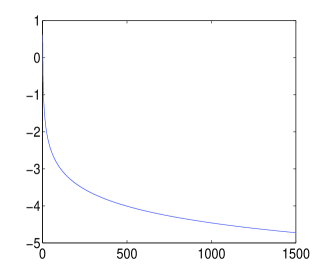
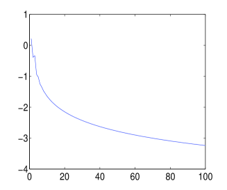
Figure 1: Graphs of $\lg|R^{m}|$ in dependence with $m$, for $\theta=1/12$, in Example 1 (left) and Example 2 (right)

One can rather easily extend the above results are to the case of the third boundary condition at $x=0$, or to the Cauchy problem where equation (1) is posed on $\mathbb{R}$. The case $\sigma<1/2$ could be also analyzed under suitable additional condition between steps $\tau$ and $h_{j}$.

6 Numerical experiments

Consider the initial-boundary value problem (1)-(3) for the simplest homogeneous heat equation where $\rho(x)\equiv 1$, $b(x)\equiv 1$, $c(x)\equiv 0$ and $f(x,t)\equiv 0$, for $0\leqslant t\leqslant T$. In Example 1, we base upon an exact solution

$$u_{1}(x,t)=\sqrt{\frac{t_{0}}{t+t_{0}}}\,e^{-(x-x_{*})^{2}/[4(t+t_{0})]}$$

with parameters $x_{*}>0$ and $t_{0}>0$ and take the data $g(t)=u_{1}(0,t)$ and $u^{0}(x)=u_{1}(x,0)$. We choose $x_{*}=1.25$, $t_{0}=0.03125$, $T=1$ and $X=2.5$. Note that $|u^{0}(x)|<3.8\cdot 10^{-6}$ for $x\geqslant X$. On Fig. 2, we demonstrate the numerical solution and its error computed for $\sigma=\frac{1}{2}$, $\theta=\frac{1}{12}$, $h=0.05$ and $\tau=\frac{1}{1500}$.

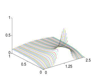
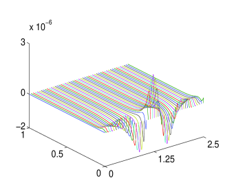
Figure 2: Example 1. The numerical solution (left) and its error (right) for $\sigma=\frac{1}{2}$, $\theta=\frac{1}{12}$, $h=0.05$ and $\tau=\frac{1}{1500}$

In Table 1, the absolute errors are given in dependence with $M$ (where $M\tau=T$) for $\theta=0$ and $\theta=\frac{1}{12}$. For $\theta=0$, they do not practically change for $M\geqslant 500$ whereas for $\theta=\frac{1}{12}$ the error continues to decrease up to $M=2000$ thus allowing to reach values of $725$ times less. Note that actually the value $U_{J}^{0}\neq 0$ has been used and the minimal reached absolute error is less than this one.

$M$	20	50	100	200	500	1000	2000
$\theta=0$	$4.39\cdot 10^{-2}$	$8.30\cdot 10^{-3}$	$1.30\cdot 10^{-3}$	$5.38\cdot 10^{-4}$	$8.63\cdot 10^{-4}$	$9.15\cdot 10^{-4}$	$9.28\cdot 10^{-4}$
$\theta=\frac{1}{12}$	$4.53\cdot 10^{-2}$	$9.50\cdot 10^{-3}$	$2.20\cdot 10^{-3}$	$4.89\cdot 10^{-4}$	$7.28\cdot 10^{-5}$	$1.35\cdot 10^{-5}$	$1.28\cdot 10^{-6}$

Table 1: Example 1. The absolute errors in dependence with $M$ for $h=0.05$

Notice that if one sets simply the Neumann boundary condition (i.e., takes $\mathcal{S}=0$) instead of the discrete TBC at $x=X$, then it is necessary to increase $X$ three times to reach the error of the same order of smallness (for the same $h$ and $\tau$); herewith the maximum absolute error is reached at $(x,t)=(X,T)$ (the corresponding graphs are omitted).

In Example 2, we take the data $g(t)=t^{2}$ and $u^{0}(x)=0$. The exact solution to such problem $u_{2}(x,t)=32t^{2}I_{4}(\xi)$ is also known and is calculated by applying the recurrence formulas [17]

$$I_{0}(\xi)=\operatorname{erfc}(\xi)\equiv\frac{2}{\sqrt{\pi}}\int_{\xi}^{\infty}e^{-\zeta^{2}}d\zeta,\ \ I_{1}(\xi)=\frac{1}{\sqrt{\pi}}e^{-\xi^{2}}-\xi\operatorname{erfc}(\xi),$$

$$I_{n}(\xi)=\frac{1}{2n}I_{n-2}(\xi)-\frac{\xi}{n}I_{n-1}(\xi),\ \ n=2,3,4,$$

where $\xi=\frac{x}{2\sqrt{t}}$. Choose $T=1$ and $X=1$.

On Fig. 3 we present the numerical solution and its error computed for $\sigma=\frac{1}{2}$, $\theta=\frac{1}{12}$, $h=0.1$ and $\tau=0.01$. In contrast to Example 1, now the solution is not close to $0$ for $x=X$. The error is maximal at the node $(x_{j},t_{m})=(h,\tau)$ (but not on the artificial boundary $x=X$). Notice that decreasing of $X$ down to $0.2$ for the same mesh steps does not increase the error (for $u^{0}=0$ and while applying namely the discrete TBC, this is natural and clear from above). Moreover, if once again one sets simply the Neumann boundary condition instead of the discrete TBC at $x=X$, then (for the same $h$ and $\tau$) the absolute error equals $0.15$ and is unacceptably large. It decreases to the same values as on Fig. 3 only when $X$ increases five times.

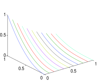
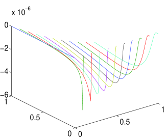
Figure 3: Example 2. The numerical solution (left) and its error (right) for $\sigma=\frac{1}{2}$, $\theta=\frac{1}{12}$, $h=0.1$ and $\tau=0.01$

On Fig. 4 we give the graphs of errors in the cases $\theta=0$ and $\theta=\frac{1}{6}$. Their forms are different and the maximum absolute errors are about two orders of magnitude greater than in the case $\theta=\frac{1}{12}$.

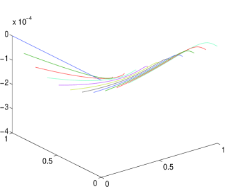
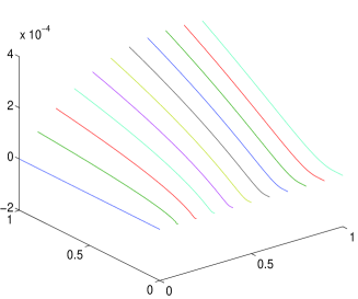
Figure 4: Example 2. The error of numerical solution in the cases $\theta=0$ (left) and $\theta=\frac{1}{6}$ (right) for $\sigma=\frac{1}{2}$, $h=0.1$ and $\tau=0.01$

In addition in Tables 2 and 3 we put the absolute errors in dependence with $M$ for $h=0.1$ and various $\theta$. For $\theta=0,\frac{1}{6}$ and $\frac{1}{4}$ the errors do not practically change already for $M\geqslant 50$; herewith their minimum values for $\theta=0$ and $\theta=\frac{1}{6}$ are close whereas for $\theta=\frac{1}{4}$ one is approximately twice larger. In contrast, for $\theta=\frac{1}{12}$ the error continues to decrease rather rapidly up to $M=500$ thus allowing to reach values about four orders of magnitude less (though it increases slightly when $M$ grows further).

$M$	5	10	20	50	100	200
$\theta=0$	$0.020$	$6.989\cdot 10^{-4}$	$4.239\cdot 10^{-4}$	$3.506\cdot 10^{-4}$	$3.402\cdot 10^{-4}$	$3.376\cdot 10^{-4}$
$\theta=\frac{1}{12}$	$0.020$	$4.948\cdot 10^{-4}$	$1.224\cdot 10^{-4}$	$1.799\cdot 10^{-5}$	$4.700\cdot 10^{-6}$	$9.300\cdot 10^{-7}$
$\theta=\frac{1}{6}$	$0.019$	$4.654\cdot 10^{-4}$	$2.565\cdot 10^{-4}$	$3.237\cdot 10^{-4}$	$3.340\cdot 10^{-4}$	$3.366\cdot 10^{-4}$
$\theta=\frac{1}{4}$	$0.019$	$4.355\cdot 10^{-4}$	$5.931\cdot 10^{-4}$	$6.613\cdot 10^{-4}$	$6.717\cdot 10^{-4}$	$6.743\cdot 10^{-4}$

Table 2: Example 2. The absolute errors in dependence with $M$ for $h=0.1$

$M$	300	400	500	600	650
$\theta=\frac{1}{12}$	$2.638\cdot 10^{-7}$	$6.797\cdot 10^{-8}$	$4.032\cdot 10^{-8}$	$8.962\cdot 10^{-8}$	$1.062\cdot 10^{-7}$

Table 3: Example 2. The absolute errors in dependence with $M\geqslant 300$ for $h=0.1$ and $\theta=\frac{1}{12}$

The study is carried out by the first author within The National Research University Higher School of Economics’ Academic Fund Program in 2012-2013, research grants No. 11-01-0051. Both authors are also supported by the Federal Agency for Science and Innovations (state contract 14.740.11.0875) and the Russian Foundation for Basic Research, project 10-01-00136.

References

1. V.A. Gordin.
Mathematical Problems in Hydrodynamical
Weather Forecasting. Computational aspects, Gidrometeoizdat: Leningrad, 1987 (in Russian).
Abridged English version: Mathematical Problems and Methods in Hydrodynamical
Weather Forecasting, Gordon and Breach: Amsterdam, 2000.
2. D. Givoli.
Numerical methods for unbounded domains.
Amsterdam: Elsevier, 1992.
3. S.V. Tsynkov.
Numerical solution of problems on unbounded domains. A review. Appl. Numer. Math. 1998; 27: 465–532.
4. V.S. Ryabenkii. Method of difference potentials and its applications.
Berlin: Springer, 2001.
5. T. Hagstrom.
New results on absorbing layers and radiation boundary conditions.
In: Topics in comput. wave propagation, M. Ainsworth et al. (eds.).
Springer, 2003. P. 1–42.
6. M. Ehrhardt.
Finite difference schemes on unbounded domains. Applications of nonstandard finite difference schemes, R.E. Mickens (ed.). Singapore: World Scientific, 2005. Vol. 2. P. 343-384.
7. M. Ehrhardt, A. Arnold.
Discrete transparent boundary conditions for the Schrödinger equation.
Riv. Mat. Univ. Parma. 2001; 6: 57-108.
9. B. Ducomet, A. Zlotnik.
On stability of the Crank-Nicolson scheme with approximate transparent boundary conditions for the Schrödinger equation. Part I.
Comm. Math. Sci. 2006; 4(4): 741-766.
10. B. Ducomet, A. Zlotnik.
On stability of the Crank-Nicolson scheme with approximate transparent boundary conditions for the Schrödinger equation. Part II.
Comm. Math. Sci. 2007; 5(2): 267-298.
11. B. Ducomet, A. Zlotnik, I. Zlotnik.
On a family of finite-difference schemes with discrete transparent boundary conditions for a generalized Schrödinger equation. Kinetic and Related Models. 2009; 2(1): 151-179.
12. M. Ehrhardt.
Discrete tranparent boundary conditions for parabolic equations. Z. Angew. Math. Mech. 1997; 77(2): 543-544.
13. A.A. Zlotnik.
On stability of the scheme with transparent boundary conditions for parabolic equations. Comput. Maths. Math. Phys. 2007; 47(4): 644 -663.
14. A.A. Zlotnik, I.A. Zlotnik. Family of finite-difference schemes with transparent boundary conditions for the nonstationary Schrödinger equation
in a semi-infinite strip. Doklady Math. 2011; 83(1): 12- 18.
15. I.A. Zlotnik.
Family of finite-difference schemes with approximate transparent boundary conditions for the generalized nonstationary Schrödinger equation in a semi-infinite strip.
Comput. Maths. Math. Phys. 2011; 51(3): 355-376.
16. M.A. Lavrentiev and B.V. Shabat.
Methods of Theory of Functions of Complex Variable,
5th edition. Nauka: Moscow, 1987 (in Russian).
17. H.S. Carslaw and J.C. Jaeger. Conduction of heat in solids, 2nd ed.
Oxford: Clarendon Press,
1986.