Classification by Boosting Differences in Input Vectors

Abstract

There are many occasions when one does not have complete information in order to classify objects into different classes, and yet it is important to do the best one can since other decisions depend on that. In astronomy, especially time-domain astronomy, this situation is common when a transient is detected and one wishes to determine what it is in order to decide if one must follow it. We propose to use the Difference Boosting Neural Network (DBNN) which can boost differences between feature vectors of different objects in order to differentiate between them. We apply it to the publicly available data of the Catalina Real-Time Transient Survey (CRTS) and present preliminary results. We also describe another use with a stellar spectral library to identify spectra based on a few features. The technique itself is more general and can be applied to a varied class of problems.

1 Introduction

It is common to have fragmented and fragmentary evidence when the sources of information are varied as well as unequal in strength. In time-domain astronomy, just like in forensic science, one tries to piece together the information in order to obtain a verdict. An object has been observed that was either not there before, or was much fainter. The only extra information available is from sporadic past observations of the same area in archival surveys that answer questions like: ‘was this seen at such and such radio frequency?’, ‘was it seen in the Sloan Digital Sky Survey?’, ‘what is the distance to the nearest galaxy?’ etc. Depending on the location of the object, and its nature, the resulting information can be sparse and very different from source to source. The Catalina Real-Time Transient Survey (CRTS) publishes the transients it finds in real-time. The events, broadcast as VOEvent packets, are ingested by Skyalert (Williams et al., 2009) where a portfolio is gathered for each object by annotating the initial information using programs that query individual surveys and archives to answer, as best as possible, a pre-determined set of questions as mentioned earlier. If one thinks of all such bits associated with an individual object as its feature, the entire input data is just a vector of features (with many, often 50-80 percent, individual features for each vector missing). Making sense of this dataset is not trivial, but classification is important (Mahabal et al. (2012), Djorgovski et al. (2011a)). Classifying the features into classes that are as unambiguous as possible, and with minimal number of false detections needs a probabilistic approach that can make full use of all available prior information.

The present work summarizes one possible method to handle such situations where the sparseness of data is diverse and patchy whereby making it difficult for existing machine learning techniques to handle them. It uses Bayesian belief update rule that can be used to progressively update the belief in the outcome based on plausible evidence. We apply the method to the CRTS transients to generate quick classification probabilities which can be revised as more data become available. We also show how it can be generalized to be used with a stellar spectral library (Valdes et al., 2004) making it especially useful in future when IFUs make available large number of spectra simultaneously.

2 Catalina Real-Time Survey

The Catalina Real-Time Transient Survey (Drake et al. (2009), Djorgovski et al. (2011b), Mahabal et al. (2011)) use data from the Catalina Sky Survey (CSS) for near-Earth objects and potential planetary hazard asteroids (NEO/PHA), conducted by Edward Beshore, Steve Larson, and their collaborators at the University of Arizona. CRTS looks for astrophysical transient and variable objects using real-time processing and carries out characterization, and distribution of these events, as well as follow-up observations of selected events.

Optical transients (OTs) are detected as sources displaying significant changes in brightness, as compared to the baseline comparison images and catalogs with significantly fainter limiting magnitudes. Data cover time baselines from 10 min to several years. The detected transients are published electronically in real time, using a variety of mechanisms. One of the methods is a Skyalert stream where additional data on the transients is gathered by harvesting archival datasets as well as information on the proximity of the source in what is termed as passive follow-up.

It is this comprehensive dataset that we make use of with DBNN in order to try to predict the nature of the transient. The training set is based upon classification by human experts. Besides the extremely sparse matrix visible to DBNN (described in the next section) the humans can use such aids as the historic light curve of the transient which a human neural network can use to trivially discriminate between SNe (single hump) versus a CV (multiple brightenings over a few years) in many cases. Such features are being incorporated into separate tools. Some derived characteristics from such aids will be incorporated into DBNN in the future. The different techniques will also be incorporated in to a fusion network.

3 Difference Boosting Neural Network (DBNN)

According to the Bayesian Theorem (von Toussaint, 2011), it is possible to start with an initial belief about the probability of occurrence of an event even when there is no compelling evidence and later update this belief periodically as new evidence is found. In the context of this paper, the initial belief is called prior and the likelihood for an observation to cause an event is called evidence. Then according to Bayesian theorem, popularly called the Bayes rule, the updated belief, or the posterior, is the product of the prior and the evidence normalized over all possibilities. Mathematically, this may be written as:

$$P(A|B)=\frac{P(B|A)\times P(A)}{\sum_{i}P(B|A_{i})\times P(A_{i})}$$ (1)

where $P(A|B)$ is the updated belief that the event A is caused by the occurrence of event B and $P(B|A)$ is the likelihood that event B may cause A. P(A) is the prior, the initial belief, which is independent of whether B is observed or not. One may call it the probability that such an event may be found even when none of the different types of evidence is seen. The index $i$ is used to normalize all the possible events including $A$ that could have produced $B$.

The beauty of the Bayesian rule is that it allows sequential updating of the belief or confidence in an outcome as more and more evidence arrives. Each time an update is made, the computed new belief becomes the new prior for the next update, thus essentially making the situation conducive for systems where one has to deal with a diverse set of inputs and come up with plausible causes that created them. The second advantage is that, all these estimates are based on the statistical distribution of the likelihoods and hence the final evidence is the probability and can be directly used as the confidence one may have in the prediction of the Bayesian classifier.

We have used a Bayesian Classifier named Difference Boosting Neural Network (Philip & Joseph, 2000) for this study. The DBNN distributes the evidence in a feature space so that every feature is associated with its likelihood as learned through a process called learning (Philip, 2009, 2010). It also estimates the prior for each evidence in individual cases that maximizes the prediction accuracy on the data used for training. This data is referred to as training data. Assuming that we have a large set of training data, it is possible to have a reasonable estimate of the prior and the likelihood even for very complex cases. After the training process, the estimated likelihoods and priors are saved for future use.

Training is usually followed by a testing cycle in which the classifier is tested with a fresh set of data that are similar but never used in the training process. This is to test for adequate learning of the classifier, in which case, the accuracy obtained on the training data and that on the test data will be comparable. If that is not the case, one has to add the failed examples also into the training data and update the likelihoods taking them into consideration. This results in a continued learning process that Bayesian classifiers can very efficiently handle. The second advantage of this progressive learning process is that the system asymptotically converges to a global optimum as the learning progresses. This similarity of Bayesian rule to human learning made Laplace comment that it is the mathematical equivalent of common sense.

Preparing the data in a format required for use by the classifier is here referred to as preprocessing. This is somewhat similar to preprocessing and data reduction that are familiar to astronomers. The preprocessing ensures that the input features are ordered in some fashion and an appropriate label is used to represent the associated class of each example in the data. Usually the number of input features may be fixed and the names of the classes all known. But the new situation narrated above has no such restriction. One can have a dynamic situation where new features are to be incorporated. For managing this new situation, we have adopted a sequence coding method in which the presence or absence of a feature is marked by a 1 or 0 in the form of a chain of binary numbers. New entries are appended to the sequence when new evidence becomes available, allowing dynamical growth of the feature vector.

Num. Code	Class
1	Cataclysmic Variable
2	Supernova
3	other
5	Blazar Outburst
6	Active Galactic Nucleus Variability
7	UVCeti Variable
8	Asteroid
9	Variable
10	Mira Variable
11	High Proper Motion Star
12	Comet
16	Nova

Table 1: The 12 different CRTS transient classes identified with numeric labels and common names.

The preprocessed data may have many missing entries depending on the list of evidence available per feature vector. The present scheme makes it possible for us to use any additional information available about an entry to make more meaningful prediction about its nature. The number of new entries and the learning based on them dynamically vary as learning progress. However, because all updating is done statistically, the subtle uncertainties and errors in the features do not affect the decision making process. The DBNN code is able to directly train and test on the preprocessed data and we describe the application of the algorithm to CRTS and stellar spectral studies in the following section.

Real $\rightarrow$	1	2	3	5	6	7	8	9	10	11	12	16	Total
Predicted
1	273	14	4	2	1	4	3	3	6	1	0	0	311
2	15	447	7	3	6	2	4	5	1	4	1	2	497
3	1	1	47	0	1	0	0	0	1	0	0	0	51
5	0	0	0	68	0	0	0	0	0	0	0	0	68
6	0	1	1	1	144	1	1	3	0	1	0	0	153
7	0	0	0	0	0	33	0	0	0	0	0	0	33
8	0	0	0	0	0	0	5	0	0	0	0	0	5
9	0	0	0	0	0	0	0	15	0	0	0	0	15
10	0	0	0	1	0	0	0	0	9	0	0	0	10
11	2	0	1	0	0	0	0	0	0	51	0	0	53
12	0	0	0	0	0	0	0	0	0	0	5	0	5
16	0	0	0	0	0	0	0	0	0	0	0	0	0
Total	291	463	59	75	152	40	13	26	17	57	6	2	1201

Table 2: The confusion matrix of the class labels: humans (Horizontal axis) against predicted (Vertical).

4 Results

The CRTS data that was used for this study has 12 distinct classification labels enumerated in Table 1 with their numerical class labels followed by the common names. The input sequence used for this study had 39 input features (including detection magnitudes, colors from archival photometry, distance to nearest star/galaxy etc.) of which 50 – 80 percent were missing in some cases. None of the cases had all 39 inputs. This forms only a subset of the data that human experts usually use for discrimination. We have not yet translated all the available information that human experts use into machine recognizable format (for example, archival light curves). This is something we want to do in the near future.

Despite these limitations, the classifier agrees with human experts in more than 90% of the cases as the graduated training progresses and it learns about the variety in the evidence. This is shown in the confusion matrix Table 2. The confusion matrix is a convenient representation showing all relevant information such as how many objects in each class were correctly identified and into which classes they were incorrectly labeled etc. It may also be used to have a rough estimate of the number density of the different classes by normalizing the totals in each class (last row) by the total number of objects (last column of the last row).

Num. Code	Object Type	Total Objects	Completeness (%)	Contamination (%)
1	Cataclysmic Variable	291	93.8	12.2
2	Supernova	463	96.5	10.1
3	Other	59	79.7	7.8
5	Blazar Outburst	75	90.7	0.0
6	Active Galactic Nucleus Variability	152	94.7	5.9
7	UVCeti Variable	40	82.5	0.0
8	Asteroid	13	38.5	0.0
9	Variable	26	57.7	0.0
10	Mira Variable	17	52.9	10
11	High Proper Motion Star	57	89.5	3.7
12	Comet	6	83.3	0.0
16	Nova	2	0.0	0.0

Table 3: Completeness and contamination details of predictions by the DBNN classifier based on Table 2 for the different type of objects in CRTS survey are shown.

Num. Code	Object Type	Total Objects	Completeness (%)	Contamination (%)
1	Cataclysmic Variable	61	63.9	35.0
2	Supernova	74	74.3	40.9
3	Other	14	0.0	100
5	Blazar Outburst	9	55.6	16.7
6	Active Galactic Nucleus Variability	26	76.9	48.7
7	UVCeti Variable	4	25.0	0.0
8	Asteroid	1	0.0	0.0
9	Variable	3	0.0	0.0
10	Mira Variable	2	0.0	0.0
11	High Proper Motion Star	5	0.0	0.0
12	Comet	1	0.0	0.0
16	Nova	0	0.0	0.0

Table 4: Classification of transients from one of the test samples. Possible reasons for relatively lower completeness are detailed in the text.

The performance of the classifier was quantified in terms of contamination and completeness. The fraction of the total number of objects in a class that were correctly recognized by the classifier is referred to as completeness and the fraction that comes as contaminants into a class due to incorrect labelling by the classifier is referred to as contamination. Both measures are indicative of how reliable the classifier is. Table 3 shows the completeness and contamination of the classifier predictions for the CRTS data taking the verdict of the human expert as reference.

As explained earlier, the classifier evaluates the Bayesian posterior probability that can be considered synonymous to the true confidence the classifier predicts. A graphical representation of the completeness and confidence measures gives a more intuitive picture of the classifier performance (Fig. 1). It may be noted that for most of the failed cases, the confidence was low indicating that they are not as reliable as the rest. It is advisable to use this as a guide to determine how safe it is to rely on low confidence predictions and to draw a cut-off line which states that anything below is unreliable. Quantification of this is in progress as more data come in.

We have also carried out tests with training the method on a smaller subset and testing on feature vectors never seen before. Due to the sheer variety in features, and the fact that a large majority of them are missing, the performance worsens (Table 4). One other important reason for this is that a few of the classes, like asteroid, comet and high proper motion stars (HPM) are not static and hence the archives do not have any information about them (at the discovery location). To incorporate that, additional features will have to be introduced. Even for many of the other classes there are not enough examples as yet. Including archival light curves will help greatly improve the SNe/CV dichotomy. All that is part of on going research, and that should be kept in mind when judging the current results.

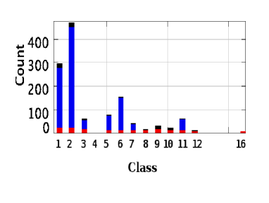
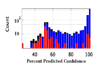
Figure 1: The plots show the performance of the classifier in predicting the nature of the objects in the CRTS survey. In the plot to the left, black colour is used to represent the total count of objects in each class while blue colour is used to represent the number of correctly recognized objects and red colour is used to indicate the number of contaminants in each class. The plot to the right shows the same with percent Bayesian confidence and the counts (in log scale to improve clarity).

As another example, the classifier was used on stellar spectra to classify them into 98 different classes as given in the Indo-US Stellar library (Valdes et al., 2004). The input features used were the major absorption lines in the spectra and the maximum flux values from four regions of the continuum in a window of 200Å centered around wavelengths 3700, 4500, 6300, 8500Å, respectively. These spectra have a coverage from 3460Å to 9464Å with a few that have missing bands in between. It was taken with a 0.9m Coud$e^{{}^{\prime}}$ telescope at Kitt Peak National Observatory in five different grating settings.

The sequence length of the extracted features used by us for this study had 32 most distinctive features in the spectra quantified by their equivalent widths and the said four flux values. We used 958 examples for training the classifier and 1104 examples for testing the learning. It was found that 88% of the classifications were in agreement with the classifications given in the catalog. The purpose of this work was only to demonstrate that the method might find some application in spectral analysis, especially for chemical abundance measures in the stellar atmosphere at a larger scale than what is possible otherwise.

5 Conclusions

We describe a new method to make use of diverse and sparse information from various sources to classify astronomical data. One practical application we found is in the case of transients where alerts need to be sent to astronomers to carry out follow up observations whenever an object that is likely to be of interest to them is detected. However, it is possible to extend the method to other applications such as spectroscopic classification where it is difficult to predefine important absorption/emission lines and we want to cluster them in a high dimensional space.

References

- Djorgovski et al. (2011a) Djorgovski, S. G., Donalek, C., Mahabal, A. A., et al. 2011a, in: Proc. CIDU 2011 Conf., eds. A. Srivasatva, et al., p. 174, NASA Ames Res. Ctr.
- Djorgovski et al. (2011b) Djorgovski, S. G., Drake, A. J., Mahabal, A. A., et al. 2011b, arXiv:1102.5004
- Drake et al. (2009) Drake, A. J., Djorgovski, S. G., Mahabal, A., et al. 2009, ApJ, 696, 870
- Mahabal et al. (2011) Mahabal, A. A., Djorgovski, S. G., Drake, A. J., et al. 2011, BASI, 39, 387
- Mahabal et al. (2012) Mahabal, A. A., Donalek, C., Djorgovski, S. G., et al. 2012, arXiv:1111.3699, in: Proc. IAU Symp. 285, New Horizons in Time Domain Astronomy, eds. E. Griffin et al., CUP, in press
- Philip & Joseph (2000) Philip, N. S., Joseph, K. B.,2000, Journal of Intelligent Data Analysis, 4, 463
-
Philip (2009)
Philip, N. S., World Conference on Nature and Biologically Inspired Computing,
(NaBIC-2009), IEEE, ISBN: 978-1-4244-5612-3. -
Philip (2010)
Philip, N. S., A Learning Algorithm based on High School Teaching Wisdom,
Paladyn Journal of Behavioral Robotics, 2010, 1(3), 160 - Valdes et al. (2004) Valdes, F., Gupta, R., Rose, J. A., Singh, H. P., & Bell, D. J. 2004, ApJS, 152, 251
- von Toussaint (2011) von Toussaint, U. 2011, Reviews of Modern Physics, 83, 943
-
Williams et al. (2009)
Williams, R. D., Djorgovski, S. G., Drake, A. J., Graham, M. J., & Mahabal, A. 2009,
Astronomical Data Analysis Software and Systems XVIII, 411, 115
Acknowledgements
The work at Caltech has been supported in part by the NSF grants AST-0407448, CNS-0540369, AST-0834235, AST-0909182 and IIS-1118041; the NASA grant 08-AISR08-0085; and by the Ajax and Fishbein Family Foundations. The first author wishes to thank Prof. Ranjan Gupta for useful discussions and acknowledges the use of Indo-US Library of Coud Feed Stellar Spectra.