On Mixtures of Skew Normal and Skew $t$-Distributions

Abstract

Finite mixtures of skew distributions have emerged as an effective tool in modelling heterogeneous data with asymmetric features. With various proposals appearing rapidly in the recent years, which are similar but not identical, the connections between them and their relative performance becomes rather unclear. This paper aims to provide a concise overview of these developments by presenting a systematic classification of the existing skew symmetric distributions into four types, thereby clarifying their close relationships. This also aids in understanding the link between some of the proposed expectation-maximization (EM) based algorithms for the computation of the maximum likelihood estimates of the parameters of the models. The final part of this paper presents an illustration of the performance of these mixture models in clustering a real dataset, relative to other non-elliptically contoured clustering methods and associated algorithms for their implementation.

1 Introduction

In recent years, non-normal distributions have received substantial interest in the statistics literature. The growing need for more flexible tools to analyze datasets that exhibit non-normal features, including asymmetry, multimodality, and heavy tails, has led to intense development in non-normal model-based methods. In particular, finite mixtures of skew distributions have emerged as a promising alternative to the traditional Gaussian mixture modelling. They have been successfully applied to numerous datasets from a wide range of fields, including the medical sciences, bioinformatics, environmetrics, engineering, economics, and financial sciences. Some recent applications of multivariate skew normal and skew $t$-mixture models include Pyne et al. (2009), Soltyk and Gupta (2011), Contreras-Reyes and Arellano-Valle (2012), and Riggi and Ingrassia (2013).

The rich literature and active discussion of skew distributions was initiated by the pioneering work of Azzalini (1985), in which the univariate skew normal distribution was introduced. Following its generalization to the multivariate skew normal distribution in Azzalini and Dalla Valle (1996), the number of contributions have grown rapidly. The concept of introducing additional parameters to regulate skewness in a distribution was subsequently extended to other parametric families, yielding the skew elliptical family; for a comprehensive survey of skew distributions, see, for example, the articles by Azzalini (2005), Arellano-Valle and Azzalini (2006), Arellano-Valle et al. (2006), and also the book edited by Genton (2004).

Besides the skew normal distribution, which plays a central role in these developments, the skew $t$-distribution has also received much attention. Being a natural extension of the $t$-distribution, the skew $t$-distribution retains reasonable tractability and is more robust against outliers than the skew normal distribution. Finite mixtures of skew normal and skew $t$-distributions have been studied by several authors, including Lin et al. (2007a, b), Pyne et al. (2009), Basso et al. (2010), Frühwirth-Schnatter and Pyne (2010), Lin (2010), Cabral et al. (2012), Vrbik and McNicholas (2012), Lee and McLachlan (2013), and Vrbik and McNicholas (2013), among others. With the existence of so many proposals, with their various characterizations of skew normal and skew $t$-distributions, it becomes rather unclear how these proposals are related to each other, and to what extent can the subtle differences between them have in practical applications.

This paper provides a concise overview of various recent developments of mixtures of skew normal and skew $t$-distributions. An illustration is given of the performance of mixtures of these distributions and some other skew mixture models in clustering a real dataset. We first present a systematic classification of multivariate skew normal and skew $t$-distributions, with special references to those used in various existing proposals of finite mixture models. We then illustrate the relative performance of these models and other related algorithms by applications to a real dataset.

Recently, Lee and McLachlan (2011) referred to the skew normal and skew $t$-distributions of Pyne et al. (2009) as ‘restricted’ skew distributions, and the class of skew elliptical distributions of Sahu et al. (2003) as having the ‘unrestricted’ form. While this terminology was later briefly discussed in Lee and McLachlan (2013) when outlining the equivalence between the skew distributions of Azzalini and Dalla Valle (1996), Pyne et al. (2009), and Basso et al. (2010), further details were not given. This papers aims to fill this gap. We shall adopt the above terminology, and expand this idea further to classify more general forms of skew distributions, namely, the ‘extended’ and ‘generalized’ forms.

The remainder of this paper is organized as follows. In Section 2, we present the classification scheme for multivariate skew normal and skew $t$-distributions, clarifying the connections between various variants. Next, we discuss the development of currently available algorithms for fitting mixtures of multivariate skew normal and skew $t$-distributions in Section 3, pointing out the equivalence between some of these algorithms. Section 4 presents an application to automated flow cytometric analysis, and comparisons are made with the results of other model-based clustering methods. Finally, some concluding remarks are given in Section 5.

2 Classification of multivariate skew normal and skew $t$-distributions

2.1 Multivariate skew normal distributions

Since the seminal article by Azzalini and Dalla Valle (1996) on the multivariate skew normal (MSN) distribution, numerous ‘extensions’ of the so-called skew normal distribution have appeared in rapid succession. The number of contributions are now so many that it is beyond the scope of this paper to include them all here. However, most of these developments can be considered as special cases of the fundamental skew normal (FUSN) distribution (Arellano-Valle and Genton, 2005), and can be systematically classified into four types, namely, the restricted, unrestricted, extended, and generalized forms.

We begin by briefly discussing the FUSN distribution, since it encompasses the first three forms of MSN distributions. The FUSN distribution itself is a generalized form of the MSN distribution. It can be generated by conditioning a multivariate normal variable on another (univariate or multivariate) random variable. Suppose $\mbox{\boldmath$Y$}_{1}\sim N_{p}(\mbox{\boldmath$0$},\boldsymbol{\Sigma})$ and $\mbox{\boldmath$Y$}_{0}$ is a $q$-dimensional random vector. Adopting the notation as used in Azzalini and Dalla Valle (1996), we let $\mbox{\boldmath$Y$}_{1}\mid\mbox{\boldmath$Y$}_{0}>\mbox{\boldmath$0$}$ be the vector $\mbox{\boldmath$Y$}_{1}$ if all elements of $\mbox{\boldmath$Y$}_{0}$ are positive and $-\mbox{\boldmath$Y$}_{1}$ otherwise. Then $\mbox{\boldmath$Y$}=\boldsymbol{\mu}+(\mbox{\boldmath$Y$}_{1}\mid\mbox{\boldmath$Y$}_{0}+\boldsymbol{\tau}>\mbox{\boldmath$0$})$ has a FUSN distribution. It is important to note that $\mbox{\boldmath$Y$}_{0}$ is not necessarily normally distributed, but in the restricted, unrestricted, and extended cases, it is restricted to be a random normal variate. The parameter $\boldsymbol{\tau}\in\mathbb{R}^{q}$, known as the extension parameter, can be viewed as a location shift for the latent variable $\mbox{\boldmath$Y$}_{0}$. When the joint distribution of $\mbox{\boldmath$Y$}_{1}$ and $\mbox{\boldmath$Y$}_{0}$ is multivariate normal, the FUSN distribution reduces to a location-scale variant of the canonical FUSN (CFUSN) distribution, given by

$$\mbox{\boldmath$Y$}=(\mbox{\boldmath$Y$}_{1}\mid\mbox{\boldmath$Y$}_{0}>\mbox{\boldmath$0$}),$$ (1)

where

$$\left[\begin{array}[]{c}\mbox{\boldmath$Y$}_{0}\\ \mbox{\boldmath$Y$}_{1}\end{array}\right]\sim N_{q+p}\left(\left[\begin{array}[]{c}\boldsymbol{\tau}\\ \boldsymbol{\mu}\end{array}\right],\left[\begin{array}[]{cc}\boldsymbol{\Gamma}&\boldsymbol{\Delta}^{T}\\ \boldsymbol{\Delta}&\boldsymbol{\Sigma}\end{array}\right]\right),$$ (2)

where $\boldsymbol{\tau}$ is a $q$-dimensional vector, $\boldsymbol{\mu}$ is $p$-dimensional vector, $\boldsymbol{\Gamma}$ is a $q\times q$ scale matrix, $\boldsymbol{\Delta}$ is an arbitrary $p\times q$ matrix, and $\boldsymbol{\Sigma}$ is a $q\times q$ scale matrix.

The restricted case corresponds to a highly specialized form of (2), where $\mbox{\boldmath$Y$}_{0}$ is restricted to be univariate (that is, $q=1$), $\boldsymbol{\tau}=0$, and $\boldsymbol{\Gamma}=1$. In the unrestricted case, both $\mbox{\boldmath$Y$}_{0}$ and $\mbox{\boldmath$Y$}_{1}$ have a $p$-dimensional normal distribution (that is, $q$=$p$). Note that the use of “restricted” here refers to restrictions on the random vector in the (conditioning-type) stochastic definition of the skew distribution. It is not a restriction on the parameter space, and so a “restricted” form of a skew distribution is not necessarily nested within its corrresponding “unrestricted” form. Indeed, the restricted and unrestricted forms coincide in the univariate case.

The extended form has no restriction on the dimensions of $\mbox{\boldmath$Y$}_{0}$, but $\boldsymbol{\tau}$ can be a non-zero vector. When $\mbox{\boldmath$Y$}_{0}$ is not normally distributed, the density of $Y$ has the generalized form. A summary of some of the existing multivariate skew normal distributions is given in Tables 1 and 2, where rMSN , uMSN, eMSN, and gMSN refer to the restricted, unrestricted, extended, and generalized version, respectively, of the multivariate skew normal distribution. The list is not exhaustive, and the names appearing in the final columns are representative examples only.

Case	Notation	Restrictions on FUSN	Examples
restricted	rMSN	$q=1$, $\tau=0$, and $\left[\begin{array}[]{c}Y_{0}\\ \mbox{\boldmath$Y$}_{1}\end{array}\right]\sim N_{1+p}$	A-MSN, B-MSN, SNI-SN, P-MSN
unrestricted	uMSN	$q=p$, $\boldsymbol{\tau}=\mbox{\boldmath$0$}$, and $\left[\begin{array}[]{c}\mbox{\boldmath$Y$}_{0}\\ \mbox{\boldmath$Y$}_{1}\end{array}\right]\sim N_{2p}$	S-MSN, G-MSN
extended	eMSN	$\boldsymbol{\tau}\neq\mbox{\boldmath$0$}$, and $\left[\begin{array}[]{c}\mbox{\boldmath$Y$}_{0}\\ \mbox{\boldmath$Y$}_{1}\end{array}\right]\sim N_{q+p}$	ESN, CSN, HSN, SUN
generalized	gMSN	$\mbox{\boldmath$Y$}_{1}$ is normally distributed	FUSN, GSN, FSN, SMSN

Table 1: Classification of multivariate skew normal distributions.

Abbreviation	Name	References
rMSN
A-MSN	Azzalini’s MSN	Azzalini and Dalla Valle (1996)
B-MSN	Branco’s MSN	Branco and Dey (2001)
SNI-SN	skew normal/independent MSN	Lachos et al. (2010)
P-MSN	Pyne’s MSN	Pyne et al. (2009)
uMSN
S-MSN	Sahu’s MSN	Sahu et al. (2003)
G-MSN	Gupta’s MSN	Gupta et al. (2004)
eMSN
ESN	Extended MSN	Azzalini and Capitanio (1999)
CSN	Closed MSN	González-Farás et al. (2004)
HSN	Hierarchical MSN	Liseo and Loperfido (2003)
SUN	Unified MSN	Arellano-Valle and Azzalini (2006)
gMSN
FUSN	Fundamental MSN	Arellano-Valle and Genton (2005)
GSN	Generalized MSN	Genton and Loperfido (2005)
FSN	Flexible MSN	Ma and Genton (2004)
SMSN	Shape mixture of MSN	Arellano-Valle et al. (2008)

Table 2: Summary of the abbreviations of skew normal distributions used in Table 1.

2.1.1 Restricted multivariate skew normal distributions

The restricted case is one of the simplest multivariate forms of the FUSN distribution. The latent variable $Y_{0}$ is assumed to be a univariate random normal variable, and its correlation with $\mbox{\boldmath$Y$}_{1}$ is controlled by $\boldsymbol{\delta}\in\mathbb{R}^{p}$. There exists two parallel forms of stochastic representation for a MSN random variable, obtained via the conditioning and convolution mechanism (Azzalini, 2005). In general, the conditioning-type stochastic representation of a restricted MSN (rMSN) distribution is given by

$$\mbox{\boldmath$Y$}=\boldsymbol{\mu}+(\mbox{\boldmath$Y$}_{1}\mid Y_{0}>0),$$ (3)

where

$$\left[\begin{array}[]{c}Y_{0}\\ \mbox{\boldmath$Y$}_{1}\end{array}\right]\sim N_{1+p}\left(\left[\begin{array}[]{c}0\\ \mbox{\boldmath$0$}\end{array}\right],\left[\begin{array}[]{cc}1&{\boldsymbol{\delta}}^{T}\\ \boldsymbol{\delta}&\boldsymbol{\Sigma}\end{array}\right]\right).$$ (4)

Alternatively, the rMSN distribution can be generated via the convolution approach, which leads to a convolution-type stochastic representation, given by

$$\mbox{\boldmath$Y$}=\boldsymbol{\mu}+\tilde{\boldsymbol{\delta}}\left|\tilde{Y}_{0}\right|+\tilde{\mbox{\boldmath$Y$}}_{1},$$ (5)

where $\tilde{Y}_{0}\sim N_{1}(0,1)$ and $\tilde{\mbox{\boldmath$Y$}}_{1}\sim N_{p}(\mbox{\boldmath$0$},\tilde{\boldsymbol{\Sigma}})$ are independent, and where $|\tilde{\mbox{\boldmath$Y$}}_{0}|$ denotes the vector whose $i$th element is given by the absolute value of the $i$th element of $\tilde{\mbox{\boldmath$Y$}}_{0}$. Note that the parameters in (5) are not identical to those in (3) and (4), but can be obtained from the latter by taking $\tilde{\boldsymbol{\delta}}=\boldsymbol{\delta}$ and $\tilde{\boldsymbol{\Sigma}}=\boldsymbol{\Sigma}-\boldsymbol{\delta}\boldsymbol{\delta}^{T}$. The connection between the pairs $(\boldsymbol{\delta},\boldsymbol{\Sigma})$ and $(\tilde{\boldsymbol{\delta}},\tilde{\boldsymbol{\Sigma}})$, are discussed in more detail in Azzalini and Capitanio (1999). The skew normal distribution proposed by Azzalini and Dalla Valle (1996), Branco and Dey (2001), Lachos et al. (2010), and Pyne et al. (2009) are identical after reparameterization, and can be formulated as the rMSN distribution.

The first multivariate skew normal distribution (A-MSN)
The first formal definition of the univariate skew normal distribution dates back to Azzalini (1985). However, its extension to the multivariate case did not appear until just over a decade later. The widely accepted ‘original’ multivariate skew normal distribution was introduced by Azzalini and Dalla Valle (1996). The density of this distribution, denoted by A-MSN$(\boldsymbol{\mu},\boldsymbol{\Sigma},\boldsymbol{\delta}_{A})$ (with some changes in notation) takes the form

$$f(\mbox{\boldmath$y$};\boldsymbol{\mu},\boldsymbol{\Sigma},\boldsymbol{\delta}_{A})=2\phi_{p}(\mbox{\boldmath$y$};\boldsymbol{\mu},\boldsymbol{\Sigma})\Phi_{1}(\boldsymbol{\delta}_{A}^{T}\mbox{\boldmath$R$}^{-1}\mbox{\boldmath$D$}^{-1}(\mbox{\boldmath$y$}-\boldsymbol{\mu});0,1-\boldsymbol{\delta}_{A}^{T}\mbox{\boldmath$R$}^{-1}\boldsymbol{\delta}_{A}),$$ (6)

where $\mbox{\boldmath$R$}=\mbox{\boldmath$D$}^{-1}\boldsymbol{\Sigma}\mbox{\boldmath$D$}^{-1}$ is the correlation matrix, $\mbox{\boldmath$D$}=\mbox{diag}(\sqrt{\Sigma}_{11},\ldots,\sqrt{\Sigma}_{pp})$ is a diagonal matrix formed by extracting the diagonal elements of $\boldsymbol{\Sigma}$, and $\Sigma_{ij}$ denotes the $ij$th entry of $\boldsymbol{\Sigma}$. We let $\phi_{p}(.;\boldsymbol{\mu},\boldsymbol{\Sigma})$ be the $p$-dimensional normal density with mean $\boldsymbol{\mu}$ and covariance matrix $\boldsymbol{\Sigma}$, and $\Phi_{1}(.;\mu,\sigma^{2})$ is the (univariate) normal distribution function of a normal variable with mean $\mu$ and variance $\sigma^{2}$. To avoid ambiguity in the notation, we have appended a subscript to some of the parameters used in different versions of the rMSN distributions throughout this paper, for example, $\boldsymbol{\delta}_{A}$ denotes the version of $\boldsymbol{\delta}$ used in the A-MSN distribution. The density (6) was obtained via the conditioning method (3), with $\mbox{\boldmath$Y$}=\boldsymbol{\mu}+\mbox{\boldmath$D$}(\mbox{\boldmath$Y$}_{1}\mid Y_{0}>0)$, where $Y_{0}$ and $\mbox{\boldmath$Y$}_{1}$ are distributed according to (4). It corresponds to the rMSN distribution in (4) with $\boldsymbol{\delta}$ replaced by $\mbox{\boldmath$D$}\boldsymbol{\delta}_{A}$. This characterization of the MSN distribution was adopted in the work of Frühwirth-Schnatter and Pyne (2010) when formulating finite mixtures of skew normal distributions, and parameter estimation was carried out using a Bayesian approach.

The skew normal distribution of Branco and Dey (B-MSN)
Branco and Dey (2001) generalized the original skew normal distribution to the class of (restricted) skew elliptical distributions. In their parameterization, the term $D$ used in the A-MSN distribution was removed, resulting in an algebraically simpler form. However, under this variant parameterization, a change in scale will affect the skewness parameter. The reader is referred to Arellano-Valle and Azzalini (2006) for a discussion on the effects of adopting this parameterization. The skew normal member of this family, denoted by B-MSN, has density

$$f(\mbox{\boldmath$y$};\boldsymbol{\mu},\boldsymbol{\delta},\boldsymbol{\Sigma})=2\phi_{p}(\mbox{\boldmath$y$};\boldsymbol{\mu},\boldsymbol{\Sigma})\Phi_{1}(\boldsymbol{\delta}^{T}\boldsymbol{\Sigma}^{-1}(\mbox{\boldmath$y$}-\boldsymbol{\mu});0,1-\boldsymbol{\delta}^{T}\boldsymbol{\Sigma}^{-1}\boldsymbol{\delta}).$$ (7)

It follows that the conditioning-type stochastic representation for $Y$ is given by $\mbox{\boldmath$Y$}=\boldsymbol{\mu}+(\mbox{\boldmath$Y$}_{1}\mid Y_{0}>0)$, where

$$\left[\begin{array}[]{c}Y_{0}\\ \mbox{\boldmath$Y$}_{1}\end{array}\right]\sim N_{1+p}\left(\left[\begin{array}[]{c}0\\ \mbox{\boldmath$0$}\end{array}\right],\left[\begin{array}[]{cc}1&\boldsymbol{\delta}^{T}\\ \boldsymbol{\delta}&\boldsymbol{\Sigma}\end{array}\right]\right),$$ (14)

and the corresponding convolution-type representation is

$$\mbox{\boldmath$Y$}=\boldsymbol{\mu}+\boldsymbol{\delta}\left|\tilde{Y}_{0}\right|+\tilde{\mbox{\boldmath$Y$}}_{1},$$ (15)

where $\tilde{Y}_{0}\sim N_{1}(0,1)$ and $\tilde{\mbox{\boldmath$Y$}}_{1}\sim N_{p}(\mbox{\boldmath$0$},\tilde{\boldsymbol{\Sigma}})$ are independent, and where $\tilde{\boldsymbol{\Sigma}}=\boldsymbol{\Sigma}-\boldsymbol{\delta}\boldsymbol{\delta}^{T}$. Note that (14) and (15) are identical to (4) and (5) respectively. It can be observed that (7) is a reparameterization of the A-MSN distribution. Replacing $\boldsymbol{\delta}$ in (7) with $\mbox{\boldmath$D$}\boldsymbol{\delta}_{A}$ recovers (6).

The skew normal/independent skew normal distribution (SNI-SN)
The skew normal Independent (SNI) distributions are, in essence, scale mixtures of the skew normal distribution. Introduced by Branco and Dey (2001), and considered further in Lachos et al. (2010), the family includes the multivariate skew normal distribution as the basic degenerate case, the density of which is given by

$$f(\mbox{\boldmath$y$};\boldsymbol{\mu},\boldsymbol{\delta}_{S},\boldsymbol{\Sigma})=2\phi_{p}(\mbox{\boldmath$y$};\boldsymbol{\mu},\boldsymbol{\Sigma})\Phi_{1}(\boldsymbol{\delta}_{S}^{T}\boldsymbol{\Sigma}^{-\frac{1}{2}}(\mbox{\boldmath$y$}-\boldsymbol{\mu});0,1-\boldsymbol{\delta}_{S}^{T}\boldsymbol{\delta}_{S}),$$ (16)

where $\boldsymbol{\Sigma}^{\frac{1}{2}}$ is the square root matrix of $\boldsymbol{\Sigma}$; that is, $\boldsymbol{\Sigma}^{\frac{1}{2}}\boldsymbol{\Sigma}^{\frac{1}{2}}=\boldsymbol{\Sigma}$. We shall adopt the notation $\mbox{\boldmath$Y$}\sim$ SNI-SN${}_{p}(\boldsymbol{\mu},\boldsymbol{\Sigma},\boldsymbol{\delta}_{S})$ when $Y$ has density (16). As with all restricted MSN distributions, the SNI-SN distribution also enjoys two parallel stochastic representations. This density is very similar to (6) and (7), and actually, is a reparameterization of them. The connection between them can be easily observed by directly comparing their stochastic representations. The two stochastic representations of the SNI-SN are given by

$$Y = \boldsymbol{\mu}+(\mbox{\boldmath$Y$}_{1}\mid Y_{0}>0),$$ (17)

and

$$Y = \boldsymbol{\mu}+\boldsymbol{\Sigma}^{\frac{1}{2}}\boldsymbol{\delta}_{S}|\tilde{Y}_{0}|+\boldsymbol{\Sigma}^{\frac{1}{2}}(I_{p}-\boldsymbol{\delta}_{S}\boldsymbol{\delta}_{S}^{T})^{\frac{1}{2}}\tilde{\mbox{\boldmath$Y$}}_{1},$$ (18)

where

$${\left[\begin{array}[]{c}Y_{0}\\ \mbox{\boldmath$Y$}_{1}\end{array}\right]\sim N_{1+p}\left(\left[\begin{array}[]{c}0\\ \mbox{\boldmath$0$}\end{array}\right],\left[\begin{array}[]{cc}1&\boldsymbol{\delta}_{S}^{T}\boldsymbol{\Sigma}^{\frac{1}{2}}\\ \boldsymbol{\Sigma}^{\frac{1}{2}}\boldsymbol{\delta}_{S}&\boldsymbol{\Sigma}\end{array}\right]\right),}$$ (25)

and $\tilde{Y}_{0}\sim N_{1}(0,1),\;\tilde{\mbox{\boldmath$Y$}}_{1}\sim N_{p}(\mbox{\boldmath$0$},\mbox{\boldmath$I$}_{p})$ are independent. It can be observed that (16) becomes identical to (7) by replacing $\boldsymbol{\delta}$ in (16) with $\boldsymbol{\Sigma}^{\frac{1}{2}}\boldsymbol{\delta}_{S}$. Cabral et al. (2012) described maximum likelihood (ML) estimation for the SNI-SN distribution via the expectation-maximization (EM) algorithm, and an extension to the mixture model was also studied.

The skew normal distribution of Pyne et al. (P-MSN)
In a study of automated flow cytometry analysis, Pyne et al. (2009) proposed yet another parametrization of the restricted skew normal distribution. This variant, hereafter referred to as the rMSN distribution (as used in Lee and McLachlan (2013)), was obtained as a ‘simplification’ of the unrestricted skew normal distribution described in Sahu et al. (2003) (see Section 2.1.2). Its density is given by

$$f\left(\mbox{\boldmath$y$};\boldsymbol{\mu},\boldsymbol{\Sigma},\boldsymbol{\delta}\right)=2\phi_{p}\left(\mbox{\boldmath$y$};\boldsymbol{\mu},\boldsymbol{\Sigma}\right)\Phi_{1}\left(\boldsymbol{\delta}^{T}\boldsymbol{\Sigma}^{-1}\left(\mbox{\boldmath$y$}-\boldsymbol{\mu}\right);0,1-\boldsymbol{\delta}^{T}\boldsymbol{\Sigma}^{-1}\boldsymbol{\delta}\right).$$ (26)

It follows that the conditioning-type stochastic representation of (26) is given by

$$\mbox{\boldmath$Y$}=\boldsymbol{\mu}+\left(\mbox{\boldmath$Y$}_{1}\mid Y_{0}>0\right),$$ (27)

where

$$\left[\begin{array}[]{c}Y_{0}\\ \mbox{\boldmath$Y$}_{1}\end{array}\right]\sim N_{1+p}\left(\left[\begin{array}[]{c}0\\ \mbox{\boldmath$0$}\end{array}\right],\left[\begin{array}[]{cc}1&\boldsymbol{\delta}^{T}\\ \boldsymbol{\delta}&\boldsymbol{\Sigma}\end{array}\right]\right),$$ (34)

and the corresponding convolution-type representation is given by

$$\mbox{\boldmath$Y$}=\boldsymbol{\mu}+\boldsymbol{\delta}|\tilde{Y}_{0}|+\tilde{\mbox{\boldmath$Y$}}_{1},$$ (35)

where again $\tilde{Y}_{0}\sim N_{1}(0,1)$ and $\tilde{\mbox{\boldmath$Y$}}_{1}\sim N_{p}(\mbox{\boldmath$0$},\tilde{\boldsymbol{\Sigma}})$ are independent, and where $\tilde{\boldsymbol{\Sigma}}=\boldsymbol{\Sigma}-\boldsymbol{\delta}\boldsymbol{\delta}^{T}$. It can be observed that (26) is identical to (7). One advantage of this parameterization is that the convolution-type representation is in a relatively simple form, and leads to a nice hierarchical form which facilitates implementation of the EM algorithm for ML parameter estimation.

For ease of reference, we include a summary of the density and stochastic representation of the above-mentioned restricted MSN distributions in Table 3 and 4, respectively.

Distribution	Density
A-MSN	$f\left(\mbox{\boldmath$y$}\right)=2\phi_{p}\left(\mbox{\boldmath$y$};\boldsymbol{\mu},\boldsymbol{\Sigma}\right)\Phi_{1}\left(\boldsymbol{\delta}_{A}^{T}\mbox{\boldmath$R$}^{-1}\mbox{\boldmath$D$}^{-1}\left(\mbox{\boldmath$y$}-\boldsymbol{\mu}\right);0,1-\boldsymbol{\delta}_{A}^{T}\mbox{\boldmath$R$}^{-1}\boldsymbol{\delta}_{A}\right)$
(1996)	$\mbox{\boldmath$D$}=\mbox{diag}(\sqrt{\Sigma_{11}},\cdots,\sqrt{\Sigma_{pp}}),\;\;\mbox{\boldmath$R$}=\mbox{\boldmath$D$}^{-1}\boldsymbol{\Sigma}\mbox{\boldmath$D$}^{-1}$
B-MSN	$f(\mbox{\boldmath$y$})=2\phi_{p}(\mbox{\boldmath$y$};\boldsymbol{\mu},\boldsymbol{\Sigma})\Phi_{1}(\boldsymbol{\delta}^{T}\boldsymbol{\Sigma}^{-1}(\mbox{\boldmath$y$}-\boldsymbol{\mu});0,1-\boldsymbol{\delta}^{T}\boldsymbol{\Sigma}^{-1}\boldsymbol{\delta})$
(2001)
P-MSN	$f(\mbox{\boldmath$y$})=2\phi_{p}(\mbox{\boldmath$y$};\boldsymbol{\mu},\boldsymbol{\Sigma})\Phi_{1}(\boldsymbol{\delta}^{T}\boldsymbol{\Sigma}^{-1}(\mbox{\boldmath$y$}-\boldsymbol{\mu});0,1-\boldsymbol{\delta}^{T}\boldsymbol{\Sigma}^{-1}\boldsymbol{\delta})$
(2009)
SNI-SN	$f(\mbox{\boldmath$y$})=2\phi_{p}(\mbox{\boldmath$y$};\boldsymbol{\mu},\boldsymbol{\Sigma})\Phi_{1}\left(\boldsymbol{\delta}_{S}^{T}\boldsymbol{\Sigma}^{-\frac{1}{2}}\left(\mbox{\boldmath$y$}-\boldsymbol{\mu}\right);0,1-\boldsymbol{\delta}_{S}^{T}\boldsymbol{\delta}_{S}\right)$
(2010)

Table 3: Summary of the densities of selected restricted forms of multivariate skew normal distributions.

Distribution	Conditioning-type representation	Convolution-type representation
A-MSN	$\mbox{\boldmath$Y$}=\boldsymbol{\mu}+\mbox{\boldmath$D$}(\mbox{\boldmath$Y$}_{1}\mid Y_{0}>0)$	$\mbox{\boldmath$Y$}=\boldsymbol{\mu}+\mbox{\boldmath$D$}\boldsymbol{\delta}_{A}|\tilde{Y}_{0}|+\tilde{\mbox{\boldmath$Y$}}_{1}$
(1996)	$\left[\begin{array}[]{c}Y_{0}\\ \mbox{\boldmath$Y$}_{1}\end{array}\right]\sim N_{1+p}\left(\left[\begin{array}[]{c}0\\ \mbox{\boldmath$0$}\end{array}\right],\left[\begin{array}[]{cc}1&\boldsymbol{\delta}_{A}^{T}\\ \boldsymbol{\delta}_{A}&\mbox{\boldmath$R$}\end{array}\right]\right)$	$\begin{array}[]{rcl}\tilde{Y}_{0}&\sim&N_{1}(0,1)\\ \tilde{\mbox{\boldmath$Y$}}_{1}&\sim&N_{p}(\mbox{\boldmath$0$},\boldsymbol{\Sigma}-\mbox{\boldmath$D$}\boldsymbol{\delta}_{A}\boldsymbol{\delta}_{A}^{T}\mbox{\boldmath$D$})\end{array}$
B-MSN	$\mbox{\boldmath$Y$}=\boldsymbol{\mu}+(\mbox{\boldmath$Y$}_{1}\mid Y_{0}>0)$	$\mbox{\boldmath$Y$}=\boldsymbol{\mu}+\boldsymbol{\delta}|\tilde{Y}_{0}|+\tilde{\mbox{\boldmath$Y$}}_{1}$
(2001)	$\left[\begin{array}[]{c}Y_{0}\\ \mbox{\boldmath$Y$}_{1}\end{array}\right]\sim N_{1+p}\left(\left[\begin{array}[]{c}0\\ \mbox{\boldmath$0$}\end{array}\right],\left[\begin{array}[]{cc}1&\boldsymbol{\delta}^{T}\\ \boldsymbol{\delta}&\boldsymbol{\Sigma}\end{array}\right]\right)$	$\begin{array}[]{rcl}\tilde{Y}_{0}&\sim&N_{1}(0,1)\\ \tilde{\mbox{\boldmath$Y$}}_{1}&\sim&N_{p}(\mbox{\boldmath$0$},\boldsymbol{\Sigma}-\boldsymbol{\delta}\boldsymbol{\delta}^{T})\end{array}$
P-MSN	$\mbox{\boldmath$Y$}=\boldsymbol{\mu}+(\mbox{\boldmath$Y$}_{1}\mid Y_{0}>0)$	$\mbox{\boldmath$Y$}=\boldsymbol{\mu}+\boldsymbol{\delta}|\tilde{Y}_{0}|+\tilde{\mbox{\boldmath$Y$}}_{1}$
(2009)	$\left[\begin{array}[]{c}Y_{0}\\ {\mbox{\boldmath$Y$}}_{1}\end{array}\right]\sim N_{1+p}\left(\left[\begin{array}[]{c}0\\ \mbox{\boldmath$0$}\end{array}\right],\left[\begin{array}[]{cc}1&\boldsymbol{\delta}^{T}\\ \boldsymbol{\delta}&\boldsymbol{\Sigma}\end{array}\right]\right)$	$\begin{array}[]{rcl}\tilde{Y}_{0}&\sim&N_{1}(0,1)\\ \tilde{\mbox{\boldmath$Y$}}_{1}&\sim&N_{p}(\mbox{\boldmath$0$},\tilde{\boldsymbol{\Sigma}})\\ \tilde{\boldsymbol{\Sigma}}&=&\boldsymbol{\Sigma}-\boldsymbol{\delta}\boldsymbol{\delta}^{T}\end{array}$
SNI-SN	$\mbox{\boldmath$Y$}=\boldsymbol{\mu}+(\mbox{\boldmath$Y$}_{1}\mid Y_{0}>0)$	$\mbox{\boldmath$Y$}=\boldsymbol{\mu}+\boldsymbol{\Sigma}^{\frac{1}{2}}\boldsymbol{\delta}_{S}|\tilde{Y}_{0}|+\boldsymbol{\Sigma}^{\frac{1}{2}}(I_{p}-\boldsymbol{\delta}_{S}\boldsymbol{\delta}_{S}^{T})^{\frac{1}{2}}\tilde{\mbox{\boldmath$Y$}}_{1}$
(2010)	$\left[\begin{array}[]{c}Y_{0}\\ {\mbox{\boldmath$Y$}}_{1}\end{array}\right]\sim N_{1+p}\left(\left[\begin{array}[]{c}0\\ \mbox{\boldmath$0$}\end{array}\right],\left[\begin{array}[]{cc}1&\boldsymbol{\delta}_{S}^{T}\boldsymbol{\Sigma}^{\frac{1}{2}}\\ \boldsymbol{\Sigma}^{\frac{1}{2}}\boldsymbol{\delta}_{S}&\boldsymbol{\Sigma}\end{array}\right]\right)$	$\begin{array}[]{rcl}\tilde{Y}_{0}&\sim&N_{1}(0,1)\\ \tilde{\mbox{\boldmath$Y$}}_{1}&\sim&N_{p}(\mbox{\boldmath$0$},\mbox{\boldmath$I$}_{p})\end{array}$

Table 4: Summary of stochastic representations of selected restricted forms of multivariate skew normal distributions.

2.1.2 Unrestricted multivariate skew normal distributions

The unrestricted case is very similar to the restricted case, except that the scalar latent variable is replaced by a $p$-dimensional normal random vector $\mbox{\boldmath$Y$}_{0}$. Accordingly, the constraint $Y_{0}>0$ becomes a set of $p$ constraints $\mbox{\boldmath$Y$}_{0}>\mbox{\boldmath$0$}$, which implies each element of $\mbox{\boldmath$Y$}_{0}$ is positive. Similar to (3) and (4), the unrestricted MSN (uMSN) distribution can be described by

$$\mbox{\boldmath$Y$}=\boldsymbol{\mu}+(\mbox{\boldmath$Y$}_{1}\mid\mbox{\boldmath$Y$}_{0}>\mbox{\boldmath$0$}),$$ (36)

where

$$\left[\begin{array}[]{c}\mbox{\boldmath$Y$}_{0}\\ \mbox{\boldmath$Y$}_{1}\end{array}\right]\sim N_{2p}\left(\left[\begin{array}[]{c}\mbox{\boldmath$0$}\\ \mbox{\boldmath$0$}\end{array}\right],\left[\begin{array}[]{cc}\mbox{\boldmath$I$}_{p}&\boldsymbol{\Delta}^{T}\\ \boldsymbol{\Delta}&\boldsymbol{\Sigma}\end{array}\right]\right).$$ (37)

Here, the skewness parameter $\boldsymbol{\Delta}$ is a $p\times p$ matrix. The convolution-type representation is analogous to (5), and is given by

$$\mbox{\boldmath$Y$}=\boldsymbol{\mu}+\tilde{\boldsymbol{\Delta}}|\tilde{\mbox{\boldmath$Y$}}_{0}|+\tilde{\mbox{\boldmath$Y$}}_{1},$$ (38)

where the random vectors $\tilde{\mbox{\boldmath$Y$}}_{0}\sim N_{p}(\mbox{\boldmath$0$},\mbox{\boldmath$I$}_{p})$ and $\tilde{\mbox{\boldmath$Y$}}_{1}\sim N_{p}(\mbox{\boldmath$0$},\tilde{\boldsymbol{\Sigma}})$ are independently distributed. The relationship between the parameters in (37) and (38) is similar to that in (3)-(5). In this case, they satisfy $\tilde{\boldsymbol{\Delta}}=\boldsymbol{\Delta}$ and $\tilde{\boldsymbol{\Sigma}}=\boldsymbol{\Sigma}-\boldsymbol{\Delta}\boldsymbol{\Delta}^{T}$. The skew normal version of Sahu et al. (2003) is an unrestricted form of the MSN distribution, with $\boldsymbol{\Delta}$ restricted to be a diagonal matrix.

The skew normal distribution of Sahu et al. (S-MSN)
In Sahu et al. (2003), skewness is introduced to a class of elliptically symmetric distributions by conditioning on a multivariate variable, which produces a class of (unrestricted) skew elliptical distribution. The multivariate skew normal distribution proposed by Sahu et al. (2003), which is a member of this family, is given by

$$f\left(\mbox{\boldmath$y$};\boldsymbol{\mu},\boldsymbol{\Sigma},\boldsymbol{\delta}\right)=2^{p}\phi_{p}\left(\mbox{\boldmath$y$};\boldsymbol{\mu},\boldsymbol{\Sigma}\right)\Phi_{p}\left(\boldsymbol{\Delta}\boldsymbol{\Sigma}^{-1}\left(\mbox{\boldmath$y$}-\boldsymbol{\mu}\right);\mbox{\boldmath$0$},\boldsymbol{\Lambda}\right),$$ (39)

where $\boldsymbol{\Delta}=\mbox{diag}\left(\boldsymbol{\delta}\right)$ and $\boldsymbol{\Lambda}=\mbox{\boldmath$I$}_{p}-\boldsymbol{\Delta}\boldsymbol{\Sigma}^{-1}\boldsymbol{\Delta}$. Observe that with this characterization of the MSN distribution, the density involves the multivariate normal distribution function, whereas the restricted forms is defined in terms of the univariate distribution instead. Accordingly, the conditioning-type stochastic representation of (39) is given by $\mbox{\boldmath$Y$}=\boldsymbol{\mu}+\left(\mbox{\boldmath$Y$}_{1}\mid\mbox{\boldmath$Y$}_{0}>\mbox{\boldmath$0$}\right)$, where

$$\left[\begin{array}[]{c}\mbox{\boldmath$Y$}_{0}\\ \mbox{\boldmath$Y$}_{1}\end{array}\right]\sim N_{2p}\left(\left[\begin{array}[]{c}\mbox{\boldmath$0$}\\ \mbox{\boldmath$0$}\end{array}\right],\left[\begin{array}[]{cc}\mbox{\boldmath$I$}_{p}&\boldsymbol{\Delta}\\ \boldsymbol{\Delta}&\boldsymbol{\Sigma}\end{array}\right]\right),$$ (46)

and the convolution-type representation is given by

$$\mbox{\boldmath$Y$}=\boldsymbol{\mu}+\boldsymbol{\Delta}|\tilde{\mbox{\boldmath$Y$}}_{0}|+\tilde{\mbox{\boldmath$Y$}}_{1},$$ (47)

where $\tilde{\mbox{\boldmath$Y$}}_{0}$ and $\tilde{\mbox{\boldmath$Y$}}_{1}$ are independent variables distributed as $\tilde{\mbox{\boldmath$Y$}}_{0}\sim N_{p}(\mbox{\boldmath$0$},\mbox{\boldmath$I$}_{p})$ and $\tilde{\mbox{\boldmath$Y$}}_{1}\sim N_{p}(\mbox{\boldmath$0$},\tilde{\boldsymbol{\Sigma}})$, respectively, and where $\tilde{\boldsymbol{\Sigma}}=\boldsymbol{\Sigma}-\boldsymbol{\Delta}^{2}$. ML estimation for the uMSN distribution, and its mixture case, is studied in Lin (2009).

2.1.3 Extended multivariate skew normal distributions

We consider now the extended skew normal (ESN) distribution, which originates from a selective sampling problem, where the variable of interest is affected by a latent variable that is truncated at an arbitrary threshold. It can be obtained via conditioning by setting $\mbox{\boldmath$Y$}=\boldsymbol{\mu}+(\mbox{\boldmath$Y$}_{1}\mid Y_{0}+\tau>0)$, where $\mbox{\boldmath$Y$}_{1}$ and $Y_{0}$ are distributed according to (4), which leads to the density

$$f(\mbox{\boldmath$y$};\boldsymbol{\mu},\boldsymbol{\Sigma},\tau)=\phi_{p}(\mbox{\boldmath$y$};\boldsymbol{\mu},\boldsymbol{\Sigma})\frac{\Phi_{1}\left(\tau+\boldsymbol{\delta}^{T}\boldsymbol{\Sigma}^{-1}(\mbox{\boldmath$y$}-\mbox{\boldmath$u$});0,1-\boldsymbol{\delta}^{T}\boldsymbol{\Sigma}^{-1}\boldsymbol{\delta}\right)}{\Phi_{1}(\tau;0,1)}.$$ (48)

This expression for an ESN distribution is due to Arnold et al. (1993), and the threshold $\tau$ is known as an extension parameter. With this additional parameter, the normalizing constant is no longer a simple fixed value (such as $2$ in the restricted case and $2^{p}$ in the unrestricted case), but a scalar value that depends on the extension parameter. Although the ESN is more complicated than the restricted and unrestricted skew normal distributions, it has nice properties not shared by these ‘no-extension’ cases, including closure under conditioning.

The ESN distribution represents one of the simplest cases of the extended form. Replacing the latent variable $Y_{0}$ with a $q$-dimensional version $\mbox{\boldmath$Y$}_{0}$ leads to the unified skew normal (SUN) distribution (Arellano-Valle and Azzalini, 2006). The SUN distribution is an attempt to unify all of the aforementioned skew normal distributions. Its conditioning-type stochastic representation is given by (1) and (2). It follows that the SUN density is given by

$$f(\mbox{\boldmath$y$};\boldsymbol{\mu},\boldsymbol{\Sigma},\boldsymbol{\Gamma},\boldsymbol{\Delta},\boldsymbol{\tau})=\phi_{p}(\mbox{\boldmath$y$};\boldsymbol{\mu},\boldsymbol{\Sigma})\frac{\Phi_{q}\left(\boldsymbol{\tau}+\boldsymbol{\Delta}^{T}\boldsymbol{\Sigma}^{-1}(\mbox{\boldmath$y$}-\boldsymbol{\mu});\mbox{\boldmath$0$},\boldsymbol{\Gamma}-\boldsymbol{\Delta}^{T}\boldsymbol{\Sigma}^{-1}\boldsymbol{\Delta}\right)}{\Phi_{q}(\boldsymbol{\tau};\mbox{\boldmath$0$},\boldsymbol{\Gamma})}.$$ (49)

Its construction can also be achieved via the convolution approach, where the $q$-dimensional latent variable $\mbox{\boldmath$Y$}_{0}$ follows a truncated normal distribution with mean $\boldsymbol{\tau}$. More specifically, let $\tilde{\mbox{\boldmath$Y$}}_{1}\sim N_{p}(0,\boldsymbol{\Sigma})$ and $\tilde{\mbox{\boldmath$Y$}}_{0}\sim TN_{q}(\boldsymbol{\tau},\boldsymbol{\Gamma})$ be independent variables, where $TN_{q}(\boldsymbol{\tau},\boldsymbol{\Gamma})$ denotes a multivariate normal variable with mean vector $\boldsymbol{\tau}$ and covariance $\boldsymbol{\Gamma}$ truncated to the positive hyperplane. Then $\mbox{\boldmath$Y$}=\boldsymbol{\mu}+\boldsymbol{\Delta}\tilde{\mbox{\boldmath$Y$}}_{0}+\tilde{\mbox{\boldmath$Y$}}_{1}$ has an extended MSN density. Note that in this case, the skewness parameter is a $p\times q$ matrix instead of the $p$-dimensional vector $\boldsymbol{\delta}$ used in the restricted and unrestricted forms of the MSN distribution.

It is not difficult to show that the SUN distribution includes the restricted MSN distributions, the unrestricted MSN distributions, and the ESN distribution as special cases. There are also various versions of MSN distributions which turns out to be equivalent to the SUN distribution, including the hierarchical skew normal (HSN) of Liseo and Loperfido (2003), the closed skew normal (CSN) of González-Farás et al. (2004), the skew normal of Gupta et al. (2004) and a location-scale variant of the canonical fundamental skew normal (CFUSN) distribution (Arellano-Valle and Genton, 2005). For a detail discussion on the equivalence between these extended forms of MSN distributions, the reader is referred to Arellano-Valle and Azzalini (2006).

2.1.4 Generalized multivariate skew normal distributions

A further generalization of the extended form of the MSN distribution is to relax the distributional assumption of the latent variable $\mbox{\boldmath$Y$}_{0}$. For the ‘generalized form’ of the MSN distribution, there are no other restrictions on the MSN density except that the symmetric part must be a multivariate normal density, that is, $\mbox{\boldmath$Y$}_{1}$ is normally distributed. This form is very general and apparently includes the other three forms discussed above. A prominent example is the fundamental skew normal distribution (FUSN), a member of the class of fundamental skew distributions considered by Arellano-Valle and Genton (2005). Its density is given by

$$f(\mbox{\boldmath$y$};\boldsymbol{\mu},\boldsymbol{\Sigma},Q_{q})=K_{q}^{-1}\phi_{p}(\mbox{\boldmath$y$};\boldsymbol{\mu},\boldsymbol{\Sigma})Q_{q}(\mbox{\boldmath$y$}),$$ (50)

where $K_{q}=E\left\{Q_{q}(\mbox{\boldmath$Y$})\right\}$ is a normalizing constant and $Q_{q}(\mbox{\boldmath$y$})$ is a skewing function. Notice that the skewing function here is not restricted to the normal family. As mentioned previously, the FUSN density can be obtained by defining $\mbox{\boldmath$Y$}=\left(\mbox{\boldmath$Y$}_{1}\mid\mbox{\boldmath$Y$}_{0}>\mbox{\boldmath$0$}\right)$, where $\mbox{\boldmath$Y$}_{1}$ follows the $p$-dimensional normal distribution with location parameter $\boldsymbol{\mu}$ and scale matrix $\boldsymbol{\Sigma}$ and $\mbox{\boldmath$Y$}_{0}$ is a $q\times 1$ random vector. Under this definition, $K_{q}$ and $Q_{q}(\mbox{\boldmath$y$})$ is given by $P(\mbox{\boldmath$Y$}_{0}>\mbox{\boldmath$0$})$ and $P(\mbox{\boldmath$Y$}_{0}>\mbox{\boldmath$0$}\mid\mbox{\boldmath$Y$}_{1})$, respectively.

An interesting special case of (50) is the location-scale variant of the so-called canonical fundamental skew normal (CFUSN) distribution, obtained by taking $\mbox{\boldmath$Y$}_{0}\sim N_{q}(\mbox{\boldmath$0$},\mbox{\boldmath$I$}_{q})$ and cov$(\mbox{\boldmath$Y$}_{1},\mbox{\boldmath$Y$}_{0})=\boldsymbol{\Delta}$. In this case, we have $\mbox{\boldmath$Y$}_{0}\mid\mbox{\boldmath$Y$}_{1}\sim N_{q}(\boldsymbol{\Delta}^{T}\boldsymbol{\Sigma}^{-1}(\mbox{\boldmath$y$}-\boldsymbol{\mu}),\boldsymbol{\Lambda})$, where $\boldsymbol{\Lambda}=\mbox{\boldmath$I$}_{q}-\boldsymbol{\Delta}^{T}\boldsymbol{\Sigma}^{-1}\boldsymbol{\Delta}$. This leads to the density

$$f(\mbox{\boldmath$y$};\boldsymbol{\mu},\boldsymbol{\Sigma},\boldsymbol{\Delta})=2^{q}\phi_{p}(\mbox{\boldmath$y$};\boldsymbol{\mu},\boldsymbol{\Sigma})\Phi_{q}(\boldsymbol{\Delta}^{T}\boldsymbol{\Sigma}^{-1}(\mbox{\boldmath$y$}-\boldsymbol{\mu});\mbox{\boldmath$0$},\boldsymbol{\Lambda}).$$ (51)

We shall write $\mbox{\boldmath$Y$}\sim CFUSN_{p,q}(\boldsymbol{\mu},\boldsymbol{\Sigma},\boldsymbol{\Delta})$. It should be noted that by taking $q=p$ and $\boldsymbol{\Delta}=\mbox{diag}(\boldsymbol{\delta})$, (51) reduces to the unrestricted skew normal density introduced by Sahu et al. (2003). Also, the CFUSN density reduces to the restricted B-MSN distribution (7) when $q=1$ and $\boldsymbol{\Delta}=\boldsymbol{\delta}$.

2.2 Multivariate skew $t$-distributions

The multivariate skew $t$-distribution is an important member of the family of skew-elliptical distributions. Like the skew normal distributions, there exists various different versions of the MST distribution, which can be nai̇vely classified into four broad forms. The MST distribution is of special interest because it offers greater flexibility than the normal distribution by combining both skewness and kurtosis in its formulation, while retaining a fair degree of tractability in an algebraic sense. This additional flexibility is much needed in some practical applications, as will be demonstrated in the example in Section 4.

In the past two decades, many variants of the multivariate skew $t$-distribution have been proposed. Some notable proposals include the skew $t$-member of Branco and Dey (2001)’s skew elliptical class, the skew $t$-distribution of Azzalini and Capitanio (2003), the skew $t$-distribution of Gupta (2003), the skew $t$-distribution of Sahu et al. (2003)’s skew elliptical class, the skew normal/independent skew $t$ (SNI-ST) distribution of Lachos et al. (2010), the closed skew $t$ (CST) distribution of Iversen (2010), and the extended skew $t$ (EST) distribution of Arellano-Valle and Genton (2010). Many of these can be considered as special cases of the fundamental skew $t$ (FUST) distribution introduced by Arellano-Valle and Genton (2005). They may be classified as ‘restricted’, ‘unrestricted’, ‘extended’, and ‘generalized’ subclasses of the FUST distribution (see Table 5).

Case	Restrictions on FUST	Examples
restricted	$q=1$, $\tau=0$ and $\left[\begin{array}[]{c}Y_{0}\\ \mbox{\boldmath$Y$}_{1}\end{array}\right]\sim t_{1+p}$	B-MST, A-MST, G-MST, P-MST, SNI-ST
unrestricted	$q=p$, $\left[\begin{array}[]{c}\mbox{\boldmath$Y$}_{0}\\ \mbox{\boldmath$Y$}_{1}\end{array}\right]\sim t_{2p}$	S-MST
extended	$\left[\begin{array}[]{c}\mbox{\boldmath$Y$}_{0}\\ \mbox{\boldmath$Y$}_{1}\end{array}\right]\sim t_{q+p}$	EST, CST, CFUST, SUT
generalized	$\mbox{\boldmath$Y$}_{1}$ is $t$-distributed	FST, GST

Table 5: Classification of MST distributions.

Abbreviation	Name	References
rMST
B-MST	Branco’s MST	Branco and Dey (2001)
A-MST	Azzalini’s MST	Azzalini and Capitanio (2003)
G-MST	Gupta’s MST	Gupta (2003)
P-MST	Pyne’s MST	Pyne et al. (2009)
SNI-ST	skew normal/independent MST	Lachos et al. (2010)
uMST
S-MST	Sahu’s MST	Sahu et al. (2003)
eMST
EST	Extended MST	Arellano-Valle and Genton (2010)
CST	Closed MST	Iversen (2010)
SUT	Unified MST	Arellano-Valle and Azzalini (2006)
gMST
FUST	Fundamental MST	Arellano-Valle and Genton (2005)
GST	Generalized MST	Genton and Loperfido (2005)
FST	Flexible MST	Ma and Genton (2004)

Table 6: Summary of the abbreviations of skew $t$-distributions used in Table 5.

2.2.1 Restricted multivariate skew $t$-distributions

The restricted skew $t$-distribution is obtained by conditioning on a univariate latent variable $Y_{0}$ being positive. The correlation between $\mbox{\boldmath$Y$}_{1}$ and $Y_{0}$ is described by the vector $\boldsymbol{\delta}$. Like the MSN distributions, the MST distributions can be obtained via a conditioning and convolution mechanism. In general, the restricted MST distribution has a conditioning-type stochastic representation given by:

$$\mbox{\boldmath$Y$}=\boldsymbol{\mu}+(\mbox{\boldmath$Y$}_{1}\mid Y_{0}>0),$$ (52)

where

$$\left[\begin{array}[]{c}Y_{0}\\ \mbox{\boldmath$Y$}_{1}\end{array}\right]\sim t_{1+p}\left(\left[\begin{array}[]{c}0\\ \mbox{\boldmath$0$}\end{array}\right],\left[\begin{array}[]{cc}1&\boldsymbol{\delta}^{T}\\ \boldsymbol{\delta}&\boldsymbol{\Sigma}\end{array}\right],\nu\right).$$ (53)

The equivalent convolution-type representation is given by

$$\mbox{\boldmath$Y$}=\boldsymbol{\mu}+\tilde{\boldsymbol{\delta}}|\tilde{Y}_{0}|+\tilde{\mbox{\boldmath$Y$}}_{1},$$ (54)

where the two random variables $\tilde{Y}_{0}$ and $\tilde{\mbox{\boldmath$Y$}}_{1}$ have a joint multivariate central $t$-distribution with scale matrix $\left[\begin{array}[]{cc}1&\mbox{\boldmath$0$}\\ \mbox{\boldmath$0$}&\tilde{\boldsymbol{\Sigma}}\end{array}\right]$ and $\nu$ degrees of freedom. The link between the pairs of parameters $(\boldsymbol{\delta},\boldsymbol{\Sigma})$ and $(\tilde{\boldsymbol{\delta}},\tilde{\boldsymbol{\Sigma}})$ is the same as that for the rMSN distribution. The skew-$t$ distribution of Branco and Dey (2001), Azzalini and Capitanio (2003), Gupta (2003), the SNI-ST, and the skew $t$-version given by Pyne et al. (2009) are equivalent to (52) up to a reparametrization.

Name	Density
B-MST	$f(\mbox{\boldmath$y$})=2t_{p}(\mbox{\boldmath$y$};\boldsymbol{\mu},\boldsymbol{\Sigma},\nu)T_{1}(\boldsymbol{\delta}^{T}\boldsymbol{\Sigma}^{-1}(\mbox{\boldmath$y$}-\boldsymbol{\mu})\sqrt{\frac{\nu+p}{\nu+d(\mbox{\boldmath$y$})}};0,1-\boldsymbol{\delta}^{T}\boldsymbol{\Sigma}^{-1}\boldsymbol{\delta},\nu+p)$
(2001)	$d(\mbox{\boldmath$y$})=(\mbox{\boldmath$y$}-\boldsymbol{\mu})^{T}\boldsymbol{\Sigma}^{-1}(\mbox{\boldmath$y$}-\boldsymbol{\mu})$
	$f\left(\mbox{\boldmath$y$}\right)=2t_{p}\left(\mbox{\boldmath$y$};\boldsymbol{\mu},\boldsymbol{\Sigma},\nu\right)T_{1}\left(\boldsymbol{\delta}_{A}^{T}\mbox{\boldmath$R$}^{-1}\mbox{\boldmath$D$}^{-1}\left(\mbox{\boldmath$y$}-\boldsymbol{\mu}\right)\sqrt{\frac{\nu+p}{\nu+d_{(}\mbox{\boldmath$y$})}};0,1-\boldsymbol{\delta}_{A}^{T}\mbox{\boldmath$R$}^{-1}\boldsymbol{\delta}_{A},\nu+p\right)$
A-MST	$\mbox{\boldmath$D$}=\mbox{diag}(\sqrt{\Sigma_{11}},\cdots,\sqrt{\Sigma_{pp}}),$
(2003)	$\mbox{\boldmath$R$}=\mbox{\boldmath$D$}^{-1}\boldsymbol{\Sigma}\mbox{\boldmath$D$}^{-1}$
	$d(\mbox{\boldmath$y$})=(\mbox{\boldmath$y$}-\boldsymbol{\mu})^{T}\boldsymbol{\Sigma}^{-1}(\mbox{\boldmath$y$}-\boldsymbol{\mu})$
G-MST	$f(\mbox{\boldmath$y$})=2t_{p}(\mbox{\boldmath$y$};\boldsymbol{\mu},\boldsymbol{\Sigma},\nu)T_{1}(\boldsymbol{\delta}_{G}^{T}(\mbox{\boldmath$y$}-\boldsymbol{\mu})\sqrt{\frac{\nu+p}{\nu+d(\mbox{\boldmath$y$})}};0,1-\boldsymbol{\delta}_{G}^{T}\boldsymbol{\Sigma}\boldsymbol{\delta}_{G},\nu+p)$
(2003)	$d(\mbox{\boldmath$y$})=(\mbox{\boldmath$y$}-\boldsymbol{\mu})^{T}\boldsymbol{\Sigma}^{-1}(\mbox{\boldmath$y$}-\boldsymbol{\mu})$
P-MST	$f(\mbox{\boldmath$y$})=2t_{p}(\mbox{\boldmath$y$};\boldsymbol{\mu},\boldsymbol{\Sigma},\nu)T_{1}\left(\boldsymbol{\delta}^{T}\boldsymbol{\Sigma}^{-1}\left(\mbox{\boldmath$y$}-\boldsymbol{\mu}\right)\sqrt{\frac{\nu+p}{\nu+d(\mbox{\boldmath$y$})}};0,1-\boldsymbol{\delta}^{T}\boldsymbol{\Sigma}^{-1}\boldsymbol{\delta},\nu+p\right)$
(2009)	$d(\mbox{\boldmath$y$})=(\mbox{\boldmath$y$}-\boldsymbol{\mu})^{T}\boldsymbol{\Sigma}^{-1}(\mbox{\boldmath$y$}-\boldsymbol{\mu})$
SNI-ST	$f(\mbox{\boldmath$y$})=2t_{p}(\mbox{\boldmath$y$};\boldsymbol{\mu},\boldsymbol{\Sigma},\nu)T_{1}\left(\boldsymbol{\delta}_{S}^{T}\boldsymbol{\Sigma}^{-\frac{1}{2}}\left(\mbox{\boldmath$y$}-\boldsymbol{\mu}\right)\sqrt{\frac{\nu+p}{\nu+d(\mbox{\boldmath$y$})}};0,1-\boldsymbol{\delta}_{S}^{T}\boldsymbol{\delta}_{S},\nu+p\right)$
(2010)	$d(\mbox{\boldmath$y$})=(\mbox{\boldmath$y$}-\boldsymbol{\mu})^{T}\boldsymbol{\Sigma}^{-1}(\mbox{\boldmath$y$}-\boldsymbol{\mu})$

Table 7: Densities of selected restricted forms of multivariate skew $t$-distributions.

Distribution	Conditioning-type representation	Convolution-type representation
B-MST	$\mbox{\boldmath$Y$}=\boldsymbol{\mu}+(\mbox{\boldmath$Y$}_{1}\mid Y_{0}>0)$	$\mbox{\boldmath$Y$}=\boldsymbol{\mu}+\boldsymbol{\delta}|\tilde{Y}_{0}|+\tilde{\mbox{\boldmath$Y$}}_{1}$
(2001)	$\left[\begin{array}[]{c}Y_{0}\\ \mbox{\boldmath$Y$}_{1}\end{array}\right]\sim t_{1+p}\left(\left[\begin{array}[]{c}0\\ \mbox{\boldmath$0$}\end{array}\right],\left[\begin{array}[]{cc}1&\boldsymbol{\delta}^{T}\\ \boldsymbol{\delta}&\boldsymbol{\Sigma}\end{array}\right],\nu\right)$	$\left[\begin{array}[]{c}\tilde{Y}_{0}\\ \tilde{\mbox{\boldmath$Y$}}_{1}\end{array}\right]\sim t_{1+p}\left(\left[\begin{array}[]{c}0\\ \mbox{\boldmath$0$}\end{array}\right],\left[\begin{array}[]{cc}1&\mbox{\boldmath$0$}\\ \mbox{\boldmath$0$}&\boldsymbol{\Sigma}-\boldsymbol{\delta}\boldsymbol{\delta}^{T}\end{array}\right],\nu\right)$
A-MST	$\mbox{\boldmath$Y$}=\boldsymbol{\mu}+\mbox{\boldmath$D$}(\mbox{\boldmath$Y$}_{1}\mid Y_{0}>0)$	$\mbox{\boldmath$Y$}=\boldsymbol{\mu}+\mbox{\boldmath$D$}\boldsymbol{\delta}_{A}|\tilde{Y}_{0}|+\tilde{\mbox{\boldmath$Y$}}_{1}$
(2003)	$\left[\begin{array}[]{c}Y_{0}\\ \mbox{\boldmath$Y$}_{1}\end{array}\right]\sim t_{1+p}\left(\left[\begin{array}[]{c}0\\ \mbox{\boldmath$0$}\end{array}\right],\left[\begin{array}[]{cc}1&\boldsymbol{\delta}_{A}^{T}\\ \boldsymbol{\delta}_{A}&\mbox{\boldmath$R$}\end{array}\right],\nu\right)$	$\left[\begin{array}[]{c}\tilde{Y}_{0}\\ \tilde{\mbox{\boldmath$Y$}}_{1}\end{array}\right]\sim t_{1+p}\left(\left[\begin{array}[]{c}0\\ \mbox{\boldmath$0$}\end{array}\right],\left[\begin{array}[]{cc}1&\mbox{\boldmath$0$}\\ \mbox{\boldmath$0$}&\boldsymbol{\Sigma}-\mbox{\boldmath$D$}\boldsymbol{\Delta}_{A}\boldsymbol{\delta}_{A}^{T}\mbox{\boldmath$D$}\end{array}\right],\nu\right)$
G-MST	$\mbox{\boldmath$Y$}=\boldsymbol{\mu}+(\mbox{\boldmath$Y$}_{1}\mid Y_{0}>0)$	$\mbox{\boldmath$Y$}=\boldsymbol{\mu}+\boldsymbol{\Sigma}\boldsymbol{\delta}_{G}|\tilde{Y}_{0}|+\tilde{\mbox{\boldmath$Y$}}_{1}$
(2003)	$\left[\begin{array}[]{c}Y_{0}\\ \mbox{\boldmath$Y$}_{1}\end{array}\right]\sim t_{1+p}\left(\left[\begin{array}[]{c}0\\ \mbox{\boldmath$0$}\end{array}\right],\left[\begin{array}[]{cc}1&\boldsymbol{\delta}_{G}^{T}\boldsymbol{\Sigma}\\ \boldsymbol{\Sigma}\boldsymbol{\delta}_{G}&\boldsymbol{\Sigma}\end{array}\right],\nu\right)$	$\left[\begin{array}[]{c}\tilde{Y}_{0}\\ \tilde{\mbox{\boldmath$Y$}}_{1}\end{array}\right]\sim t_{1+p}\left(\left[\begin{array}[]{c}0\\ \mbox{\boldmath$0$}\end{array}\right],\left[\begin{array}[]{cc}1&\mbox{\boldmath$0$}\\ \mbox{\boldmath$0$}&\boldsymbol{\Sigma}-\boldsymbol{\Sigma}\boldsymbol{\delta}_{G}\boldsymbol{\delta}_{G}^{T}\boldsymbol{\Sigma}\end{array}\right],\nu\right)$
P-MST	$\mbox{\boldmath$Y$}=\boldsymbol{\mu}+(\mbox{\boldmath$Y$}_{1}\mid Y_{0}>0)$	$\mbox{\boldmath$Y$}=\boldsymbol{\mu}+\boldsymbol{\delta}|\tilde{Y_{0}}|+\tilde{\mbox{\boldmath$Y$}}_{1}$
(2009)	$\left[\begin{array}[]{c}{Y}_{0}\\ \mbox{\boldmath$Y$}_{1}\end{array}\right]\sim t_{1+p}\left(\left[\begin{array}[]{c}0\\ \mbox{\boldmath$0$}\end{array}\right],\left[\begin{array}[]{cc}1&\boldsymbol{\delta}^{T}\\ \boldsymbol{\delta}&\boldsymbol{\Sigma}\end{array}\right],\nu\right)$	$\begin{array}[]{c}\left[\begin{array}[]{c}\tilde{Y}_{0}\\ \tilde{\mbox{\boldmath$Y$}}_{1}\end{array}\right]\sim t_{1+p}\left(\left[\begin{array}[]{c}0\\ \mbox{\boldmath$0$}\end{array}\right],\left[\begin{array}[]{cc}1&\mbox{\boldmath$0$}\\ \mbox{\boldmath$0$}&\tilde{\boldsymbol{\Sigma}}\end{array}\right],\nu\right)\\ \tilde{\boldsymbol{\Sigma}}=\boldsymbol{\Sigma}-\boldsymbol{\delta}\boldsymbol{\delta}^{T}\end{array}$
SNI-ST	$\mbox{\boldmath$Y$}=\boldsymbol{\mu}+(\mbox{\boldmath$Y$}_{1}\mid Y_{0}>0)$	$\mbox{\boldmath$Y$}=\boldsymbol{\mu}+\boldsymbol{\Sigma}^{\frac{1}{2}}\boldsymbol{\delta}_{S}|\tilde{Y}_{0}|+\boldsymbol{\Sigma}^{\frac{1}{2}}(I_{p}-\boldsymbol{\delta}_{S}\boldsymbol{\delta}_{S}^{T})^{\frac{1}{2}}\tilde{\mbox{\boldmath$Y$}}_{1}$
(2010)	$\left[\begin{array}[]{c}{Y}_{0}\\ {\mbox{\boldmath$Y$}}_{1}\end{array}\right]\sim t_{1+p}\left(\left[\begin{array}[]{c}0\\ \mbox{\boldmath$0$}\end{array}\right],\left[\begin{array}[]{cc}1&\boldsymbol{\delta}_{S}^{T}\boldsymbol{\Sigma}^{\frac{1}{2}}\\ \boldsymbol{\Sigma}^{\frac{1}{2}}\boldsymbol{\delta}_{S}&\boldsymbol{\Sigma}\end{array}\right],\nu\right)$	$\left[\begin{array}[]{c}\tilde{Y}_{0}\\ \tilde{\mbox{\boldmath$Y$}}_{1}\end{array}\right]\sim t_{1+p}\left(\left[\begin{array}[]{c}0\\ \mbox{\boldmath$0$}\end{array}\right],\left[\begin{array}[]{cc}1&\mbox{\boldmath$0$}\\ \mbox{\boldmath$0$}&\mbox{\boldmath$I$}_{p}\end{array}\right],\nu\right)$

Table 8: Stochastic representations of selected restricted forms of multivariate skew $t$-distributions.

The skew t-distribution of Branco and Dey (B-MST)
The skew elliptical class of Branco and Dey (2001) includes a skew $t$-distribution, which is a special case of a scale mixture of the B-MSN distribution. Its density is given by

$$f(\mbox{\boldmath$y$}) = 2t_{p}(\mbox{\boldmath$y$};\boldsymbol{\mu},\boldsymbol{\Sigma},\nu)\;$$ (55)

$$T_{1}\left(\boldsymbol{\delta}^{T}\boldsymbol{\Sigma}^{-1}(\mbox{\boldmath$y$}-\boldsymbol{\mu})\sqrt{\frac{\nu+p}{\nu+d(\mbox{\boldmath$y$})}};0,1-\boldsymbol{\delta}^{T}\boldsymbol{\Sigma}^{-1}\boldsymbol{\delta},\nu+p\right),$$

where $d(\mbox{\boldmath$y$})=(\mbox{\boldmath$y$}-\boldsymbol{\mu})^{T}\boldsymbol{\Sigma}^{-1}(\mbox{\boldmath$y$}-\boldsymbol{\mu})$ is the squared Mahalanobis distance between $y$ and $\boldsymbol{\mu}$ with respect to $\boldsymbol{\Sigma}$. Here, we let $t_{p}(.;\boldsymbol{\mu},\boldsymbol{\Sigma},\nu)$ denote the $p$-dimensional $t$-density with location vector $\boldsymbol{\mu}$, scale matrix $\boldsymbol{\Sigma}$, and degrees of freedom $\nu$, and $T_{1}(.;\mu,\sigma^{2},\nu)$ denote the distribution function of the (univariate) $t$-distribution with mean $\mu$, variance $\sigma^{2}$ and degrees of freedom $\nu$. It can be observed from representation (55) that the multivariate skew $t$-distribution converges to the B-MSN density (7) when the degrees of freedom $\nu$ approaches infinity.

It follows that $Y$ has a conditioning-type representation given by $\mbox{\boldmath$Y$}=\boldsymbol{\mu}+(\mbox{\boldmath$Y$}_{1}\mid Y_{0}>0)$, where

$$\left[\begin{array}[]{c}Y_{0}\\ \mbox{\boldmath$Y$}_{1}\end{array}\right]\sim t_{1+p}\left(\left[\begin{array}[]{c}0\\ \mbox{\boldmath$0$}\end{array}\right],\left[\begin{array}[]{cc}1&\boldsymbol{\delta}^{T}\\ \boldsymbol{\delta}&\boldsymbol{\Sigma}\end{array}\right],\nu\right),$$ (62)

and a corresponding convolution-type representation given by

$$\mbox{\boldmath$Y$}=\boldsymbol{\mu}+\boldsymbol{\delta}\left|\tilde{Y}_{0}\right|+\tilde{\mbox{\boldmath$Y$}}_{1},$$ (63)

where

$$\left[\begin{array}[]{c}\tilde{Y}_{0}\\ \tilde{\mbox{\boldmath$Y$}}_{1}\end{array}\right]\sim t_{1+p}\left(\left[\begin{array}[]{c}0\\ \mbox{\boldmath$0$}\end{array}\right],\left[\begin{array}[]{cc}1&\mbox{\boldmath$0$}\\ \mbox{\boldmath$0$}&\boldsymbol{\Sigma}-\boldsymbol{\delta}\boldsymbol{\delta}^{T}\end{array}\right],\nu\right).$$ (70)

It can be seen that (62) is identical to (53).

The skew t-distribution of Azzalini and Capitanio (A-MST)
Azzalini and Capitanio (2003) extended the A-MSN distribution of Azzalini and Dalla Valle (1996) to the skew $t$-case. Its density is given by

$$f\left(\mbox{\boldmath$y$}\right) = 2t_{p}\left(\mbox{\boldmath$y$};\boldsymbol{\mu},\boldsymbol{\Sigma},\nu\right)$$

$$T_{1}\left(\boldsymbol{\delta}_{A}^{T}\mbox{\boldmath$R$}^{-1}\mbox{\boldmath$D$}^{-1}\left(\mbox{\boldmath$y$}-\boldsymbol{\mu}\right)\sqrt{\frac{\nu+p}{\nu+d(\mbox{\boldmath$y$})}};0,1-\boldsymbol{\delta}_{A}^{T}\mbox{\boldmath$R$}^{-1}\boldsymbol{\delta}_{A},\nu+p\right),$$

where $d(\mbox{\boldmath$y$})=(\mbox{\boldmath$y$}-\boldsymbol{\mu})^{T}\boldsymbol{\Sigma}^{-1}(\mbox{\boldmath$y$}-\boldsymbol{\mu})$, $\mbox{\boldmath$R$}=\mbox{\boldmath$D$}^{-1}\boldsymbol{\Sigma}\mbox{\boldmath$D$}^{-1}$ is the correlation matrix, and $D$ is the diagonal matrix created by extracting the diagonal elements of $\boldsymbol{\Sigma}$. Note again that the parameter $\boldsymbol{\delta}$ in (LABEL:AzzaST) is marked with a subscript $A$ to indicate that it is different to the definition used in (55) and other rMST distributions. The A-MST density (LABEL:AzzaST) can be obtained by a conditioning mechanism, similar to the A-MSN distribution, by setting $\mbox{\boldmath$Y$}=\boldsymbol{\mu}+\mbox{\boldmath$D$}(\mbox{\boldmath$Y$}_{1}\mid Y_{0}>0)$, where

$$\left[\begin{array}[]{c}Y_{0}\\ \mbox{\boldmath$Y$}_{1}\end{array}\right]\sim t_{1+p}\left(\left[\begin{array}[]{c}0\\ \mbox{\boldmath$0$}\end{array}\right],\left[\begin{array}[]{cc}1&\boldsymbol{\delta}_{A}^{T}\\ \boldsymbol{\delta}_{A}&\mbox{\boldmath$R$}\end{array}\right],\nu\right).$$ (78)

A parallel representation of (LABEL:AzzaST) via the convolution mechanism is given by

$$\mbox{\boldmath$Y$}=\boldsymbol{\mu}+\mbox{\boldmath$D$}\boldsymbol{\delta}_{A}\left|\tilde{Y}_{0}\right|+\tilde{\mbox{\boldmath$Y$}}_{1},$$ (79)

where

$$\left[\begin{array}[]{c}\tilde{Y}_{0}\\ \tilde{\mbox{\boldmath$Y$}}_{1}\end{array}\right]\sim t_{1+p}\left(\left[\begin{array}[]{c}0\\ \mbox{\boldmath$0$}\end{array}\right],\left[\begin{array}[]{cc}1&\mbox{\boldmath$0$}\\ \mbox{\boldmath$0$}&\boldsymbol{\Sigma}-\mbox{\boldmath$D$}\boldsymbol{\delta}_{A}\boldsymbol{\delta}_{A}^{T}\mbox{\boldmath$D$}\end{array}\right],\nu\right).$$ (86)

In this parameterization, the scale matrix $\boldsymbol{\Sigma}$ is partitioned into $D$$R$$D$, making the skewness parameter invariant to a change of scale. Setting $\boldsymbol{\delta}$ in (55) to $\mbox{\boldmath$D$}\boldsymbol{\delta}_{A}$ leads to the B-MST distribution (LABEL:AzzaST). This characterization of the rMST distribution was considered by Frühwirth-Schnatter and Pyne (2010) to define a skew $t$-mixture model, and an algorithm for parameter estimation was formulated using a Bayesian framework.

The skew $t$-distribution of Gupta (G-MST)
In Gupta (2003), another version of the restricted skew $t$-distribution is defined, starting from the A-MSN distribution of Azzalini and Dalla Valle (1996). In this parameterization, the scale matrix $\boldsymbol{\Sigma}$ is not factored into the product $D$$R$$D$, and the parameter $\boldsymbol{\delta}_{A}$ is replaced by $\mbox{\boldmath$D$}^{-1}\boldsymbol{\Sigma}\boldsymbol{\delta}_{G}$, leading to a density in a slightly simpler algebraic form, given by

$$f(\mbox{\boldmath$y$})=2t_{p}(\mbox{\boldmath$y$};\boldsymbol{\mu},\boldsymbol{\Sigma},\nu)T_{1}\left(\boldsymbol{\delta}_{G}^{T}(\mbox{\boldmath$y$}-\boldsymbol{\mu})\sqrt{\frac{\nu+p}{\nu+d(\mbox{\boldmath$y$})}};0,1-\boldsymbol{\delta}_{G}^{T}\boldsymbol{\Sigma}\boldsymbol{\delta}_{G},\nu+p\right),$$ (87)

where, as before, $d(\mbox{\boldmath$y$})=(\mbox{\boldmath$y$}-\boldsymbol{\mu})^{T}\boldsymbol{\Sigma}^{-1}(\mbox{\boldmath$y$}-\boldsymbol{\mu})$. Note that (87) is identical to (55) if we rewrite $\boldsymbol{\delta}$ in (55) as $\boldsymbol{\Sigma}\boldsymbol{\delta}_{G}$. It follows that the stochastic representation of the G-MST distribution (87) can be expressed as

$$Y = \boldsymbol{\mu}+\left(\mbox{\boldmath$Y$}_{1}\mid Y_{0}>0\right),$$ (88)

where

$$\left[\begin{array}[]{c}Y_{0}\\ \mbox{\boldmath$Y$}_{1}\end{array}\right]\sim t_{1+p}\left(\left[\begin{array}[]{c}0\\ \mbox{\boldmath$0$}\end{array}\right],\left[\begin{array}[]{cc}1&\boldsymbol{\delta}_{G}^{T}\boldsymbol{\Sigma}\\ \boldsymbol{\Sigma}\boldsymbol{\delta}_{G}&\boldsymbol{\Sigma}\end{array}\right],\nu\right).$$ (95)

The skew normal/independent skew $t$-distribution (SNI-ST)
The skew $t$ member of the SNI class, denoted by SNI-ST, is introduced as a scale mixture of SNI-SN distributions with gamma scale factor (Lachos et al., 2010). Its density is given by

$$f(\mbox{\boldmath$y$}) = 2t_{p}(\mbox{\boldmath$y$};\boldsymbol{\mu},\boldsymbol{\Sigma},\nu)$$ (96)

$$T_{1}\left(\boldsymbol{\delta}_{S}^{T}\boldsymbol{\Sigma}^{-\frac{1}{2}}\left(\mbox{\boldmath$y$}-\boldsymbol{\mu}\right)\sqrt{\frac{\nu+p}{\nu+d(\mbox{\boldmath$y$})}};0,1-\boldsymbol{\delta}_{S}^{T}\boldsymbol{\delta}_{S},\nu+p\right),$$

where $d(\mbox{\boldmath$y$})=(\mbox{\boldmath$y$}-\boldsymbol{\mu})^{T}\boldsymbol{\Sigma}^{-1}(\mbox{\boldmath$y$}-\boldsymbol{\mu})$, and $\boldsymbol{\Sigma}^{\frac{1}{2}}$ is the square root matrix of $\boldsymbol{\Sigma}$; that is, $\boldsymbol{\Sigma}^{\frac{1}{2}}\boldsymbol{\Sigma}^{\frac{1}{2}}=\boldsymbol{\Sigma}$. The SNI-ST distribution (96) can be generated by taking $\mbox{\boldmath$Y$}=\boldsymbol{\mu}+(\mbox{\boldmath$Y$}_{1}\mid Y_{0}>0)$, where

$$\left[\begin{array}[]{c}Y_{0}\\ \mbox{\boldmath$Y$}_{1}\end{array}\right]\sim t_{1+p}\left(\left[\begin{array}[]{c}0\\ \mbox{\boldmath$0$}\end{array}\right],\left[\begin{array}[]{cc}1&\boldsymbol{\delta}_{S}^{T}\boldsymbol{\Sigma}^{\frac{1}{2}}\\ \boldsymbol{\Sigma}^{\frac{1}{2}}\boldsymbol{\delta}_{S}&\boldsymbol{\Sigma}\end{array}\right],\nu\right),$$ (103)

and the corresponding convolution-type representation is given by

$$\mbox{\boldmath$Y$}=\boldsymbol{\mu}+\boldsymbol{\Sigma}^{\frac{1}{2}}\boldsymbol{\delta}_{S}|\tilde{Y}_{0}|+\boldsymbol{\Sigma}^{\frac{1}{2}}(I_{p}-\boldsymbol{\delta}_{S}\boldsymbol{\delta}_{S}^{T})^{\frac{1}{2}}\tilde{\mbox{\boldmath$Y$}}_{1},$$ (104)

where $\tilde{Y}_{0}$ and $\tilde{\mbox{\boldmath$Y$}}_{1}$ are jointly distributed as

$$\left[\begin{array}[]{c}\tilde{Y}_{0}\\ \tilde{\mbox{\boldmath$Y$}}_{1}\end{array}\right]\sim t_{1+p}\left(\left[\begin{array}[]{c}0\\ \mbox{\boldmath$0$}\end{array}\right],\left[\begin{array}[]{cc}1&\mbox{\boldmath$0$}\\ \mbox{\boldmath$0$}&\mbox{\boldmath$I$}_{p}\end{array}\right],\nu\right)$$ (111)

It can observed that (96) is equivalent to (55) by replacing $\boldsymbol{\delta}$ in (55) with $\boldsymbol{\Sigma}^{\frac{1}{2}}\boldsymbol{\delta}_{S}$. Basso et al. (2010) and Cabral et al. (2012) studied, respectively, finite mixtures of univariate and multivariate SNI-ST distributions, and derived an ECME algorithm for computing the ML estimates of the model parameters.

The skew $t$-distribution of Pyne et al. (P-MST)
In Pyne et al. (2009), a restricted variant of Sahu et al. (2003)’s skew $t$-distribution was introduced, and its density is given by

$$f(\mbox{\boldmath$y$}) = 2t_{p}(\mbox{\boldmath$y$};\boldsymbol{\mu},\boldsymbol{\Sigma},\nu)$$ (112)

$$T_{1}\left(\boldsymbol{\delta}^{T}\boldsymbol{\Sigma}^{-1}\left(\mbox{\boldmath$y$}-\boldsymbol{\mu}\right)\sqrt{\frac{\nu+p}{\nu+d(\mbox{\boldmath$y$})}};0,1-\boldsymbol{\delta}^{T}\boldsymbol{\Sigma}^{-1}\boldsymbol{\delta},\nu+p\right),$$

where $d(\mbox{\boldmath$y$})=(\mbox{\boldmath$y$}-\boldsymbol{\mu})^{T}\boldsymbol{\Sigma}^{-1}(\mbox{\boldmath$y$}-\boldsymbol{\mu})$. We shall refer to the density (112) as the rMST distribution. This distribution has straightforward conditioning and convolution-type stochastic representations, given by

$$\mbox{\boldmath$Y$}=\boldsymbol{\mu}+\left(\mbox{\boldmath$Y$}_{1}\mid Y_{0}>0\right),$$

and

$$\mbox{\boldmath$Y$}=\boldsymbol{\mu}+\boldsymbol{\delta}|\tilde{Y}_{0}|+\tilde{\mbox{\boldmath$Y$}}_{1},$$

respectively, where

$$\left[\begin{array}[]{c}Y_{0}\\ \mbox{\boldmath$Y$}_{1}\end{array}\right]\sim t_{1+p}\left(\left[\begin{array}[]{c}0\\ \mbox{\boldmath$0$}\end{array}\right],\left[\begin{array}[]{cc}1&\boldsymbol{\delta}^{T}\\ \boldsymbol{\delta}&\boldsymbol{\Sigma}\end{array}\right],\nu\right),$$ (119)

and

$$\left[\begin{array}[]{c}\tilde{Y}_{0}\\ \tilde{\mbox{\boldmath$Y$}}_{1}\end{array}\right]\sim t_{1+p}\left(\left[\begin{array}[]{c}0\\ \mbox{\boldmath$0$}\end{array}\right],\left[\begin{array}[]{cc}1&\mbox{\boldmath$0$}\\ \mbox{\boldmath$0$}&\tilde{\boldsymbol{\Sigma}}\end{array}\right],\nu\right),$$ (126)

and where $\tilde{\boldsymbol{\Sigma}}=\boldsymbol{\Sigma}-\boldsymbol{\delta}\boldsymbol{\delta}^{T}$. It can be observed that the restricted MST (112) is identical to (52). Mixtures of rMST distributions was first studied by Pyne et al. (2009), and a closed-form implementation of the EM algorithm was outlined. Vrbik and McNicholas (2012) subsequently provided an alternative exact implementation.

A summary of the correspondence between the parameters used in various versions of the restricted MST distribution is given in Table 9. Their densities and stochastic representations are listed in Tables 7 and 8.

rMST	$\boldsymbol{\delta}$	$\boldsymbol{\Sigma}$
B-MST	$\boldsymbol{\delta}$	$\boldsymbol{\Sigma}$
A-MST	$\mbox{\boldmath$D$}\boldsymbol{\delta}_{A}$	$\boldsymbol{\Sigma}$
G-MST	$\boldsymbol{\Sigma}\boldsymbol{\delta}_{G}$	$\boldsymbol{\Sigma}$
P-MST	$\boldsymbol{\delta}$	$\boldsymbol{\Sigma}$
SI-ST	$\boldsymbol{\Sigma}^{\frac{1}{2}}\boldsymbol{\delta}_{S}$	$\boldsymbol{\Sigma}$

Table 9: Correspondence between the parametrization of the restricted forms of MST distributions.

2.2.2 Unrestricted multivariate skew $t$-distributions

In the unrestricted case, the latent variable $\mbox{\boldmath$Y$}_{0}$ is a $p$-dimensional random vector following a $t$-distribution. Under this setting, $Y$ is given in terms of the conditional distribution of $\mbox{\boldmath$Y$}_{1}$ given $\mbox{\boldmath$Y$}_{0}$ is positive. The condition $\mbox{\boldmath$Y$}_{0}>\mbox{\boldmath$0$}$ implies that each element of $\mbox{\boldmath$Y$}_{0}$ is greater than zero. Similar to (52), the unrestricted MST distribution takes the form

$$\mbox{\boldmath$Y$}=\boldsymbol{\mu}+\left(\mbox{\boldmath$Y$}_{1}\mid\mbox{\boldmath$Y$}_{0}>\mbox{\boldmath$0$}\right),$$ (127)

where

$$\left[\begin{array}[]{c}\mbox{\boldmath$Y$}_{0}\\ \mbox{\boldmath$Y$}_{1}\end{array}\right]\sim t_{2p}\left(\left[\begin{array}[]{c}\mbox{\boldmath$0$}\\ \mbox{\boldmath$0$}\end{array}\right],\left[\begin{array}[]{cc}\mbox{\boldmath$I$}_{p}&\boldsymbol{\Delta}\\ \boldsymbol{\Delta}&\boldsymbol{\Sigma}\end{array}\right],\nu\right).$$ (134)

The analogous convolution-type representation is given by

$$\mbox{\boldmath$Y$}=\boldsymbol{\mu}+\boldsymbol{\Delta}|\tilde{\mbox{\boldmath$Y$}}_{0}|+\tilde{\mbox{\boldmath$Y$}_{1}},$$ (135)

where the two random vectors $\tilde{\mbox{\boldmath$Y$}}_{0}$ and $\tilde{\mbox{\boldmath$Y$}}_{1}$ are jointly distributed as

$$\left[\begin{array}[]{c}\tilde{Y}_{0}\\ \tilde{\mbox{\boldmath$Y$}}_{1}\end{array}\right]\sim t_{2p}\left(\left[\begin{array}[]{c}\mbox{\boldmath$0$}\\ \mbox{\boldmath$0$}\end{array}\right],\left[\begin{array}[]{cc}\mbox{\boldmath$I$}_{p}&\mbox{\boldmath$0$}\\ \mbox{\boldmath$0$}&\tilde{\boldsymbol{\Sigma}}\end{array}\right],\nu\right),$$ (142)

and where $\tilde{\boldsymbol{\Sigma}}=\boldsymbol{\Sigma}-\boldsymbol{\Delta}^{2}$.

This form of the MST distribution is studied in detail in Sahu et al. (2003), and its density is given by

$$f(\mbox{\boldmath$y$})=2^{p}\;t_{p}(\mbox{\boldmath$y$};\boldsymbol{\mu},\boldsymbol{\Sigma},\nu)\;T_{p}\left(\boldsymbol{\Delta}\boldsymbol{\Sigma}^{-1}(\mbox{\boldmath$y$}-\boldsymbol{\mu})\sqrt{\frac{\nu+p}{\nu+d(\mbox{\boldmath$y$})}};\mbox{\boldmath$0$},\boldsymbol{\Lambda},\nu+p\right),$$ (143)

where $\boldsymbol{\Delta}=\mbox{diag}\left(\boldsymbol{\delta}\right)$, $\boldsymbol{\Lambda}=\mbox{\boldmath$I$}_{p}-\boldsymbol{\Delta}\boldsymbol{\Sigma}^{-1}\boldsymbol{\Delta}$, and $d(\mbox{\boldmath$y$})=(\mbox{\boldmath$y$}-\boldsymbol{\mu})^{T}\boldsymbol{\Sigma}^{-1}(\mbox{\boldmath$y$}-\boldsymbol{\mu})$. ML estimation for the unrestricted characterization of the MST distribution is a difficult computational problem. Lin (2010) used a Monte Carlo (MC) E-step when implementing the EM algorithm. Later, Lee and McLachlan (2011), Ho et al. (2012), and Lee and McLachlan (2013) proposed an improved implementation using a truncated moments approach.

It is important to point out that, although the rMST distribution (112) was originally obtained as a restricted variant of the uMST distribution (143), and both can be constructed by the conditioning and convolution approach, where (143) uses a $p$-dimensional latent variable instead of a scalar latent variable used in (112), the density (143) does not incorporate (112). The two densities are equivalent only in the univariate case.

2.2.3 Extended multivariate skew $t$-distributions

There are parallel versions of the ESN and the SUN distributions for the skew $t$-distribution, known as the extended skew $t$ (EST) distribution (Arellano-Valle and Genton, 2010) and the unified skew $t$ (SUT) distribution (Arellano-Valle and Azzalini, 2006), respectively. Their links are analogous to those for the skew normal distributions in Section 2.1.3.

2.2.4 Generalized multivariate skew $t$-distributions

Similar to the generalized forms of the MSN distribution, analogous extensions to the skew $t$ case can be constructed. They include the FUST distribution and other subclasses of it, as well as the generalized form of the $t$-distribution put forward by Arellano-Valle et al. (2006), known as the selection $t$-distribution.

3 Mixtures of multivariate skew normal and skew
$t$-distributions

In a mixture model context, the underlying population can be conceptualized as being composed of a finite number of subpopulations. Let $\mbox{\boldmath$Y$}={\mbox{\boldmath$Y$}_{1},\ldots,\mbox{\boldmath$Y$}_{n}}$ denote a random sample of $n$ observations. Then the probability density function (pdf) of the $g$ component finite mixture model takes the form

$$f(\mbox{\boldmath$y$};\boldsymbol{\Psi})=\sum_{h=1}^{g}\pi_{h}f(\mbox{\boldmath$y$};\boldsymbol{\theta}_{h}),$$ (144)

where $f(\mbox{\boldmath$y$};\boldsymbol{\theta}_{h})$ is the density of the $h$th population, and $\pi_{h}$ its corresponding weight. The mixing proportions $\pi_{h}$ satisfies $\pi_{h}\geq 0$ $(h=1,\ldots,h)$, and $\sum_{h=1}^{g}\pi_{h}=1$. The vector $\boldsymbol{\theta}_{h}$ consists of the unknown parameters in the postulated form of the $h$th component of the mixture model, and $\boldsymbol{\Psi}=\left(\pi_{1},\ldots,\pi_{g-1},\boldsymbol{\theta}_{q},\ldots,\boldsymbol{\theta}_{g}\right)^{T}$ denotes the vector containing all unknown parameters.

Computation of the ML estimates of the model parameters is typically achieved through the EM algorithm. Under the EM framework, the observed data vector is regarded as incomplete, and latent component labels (and possibly other latent variables as needed) are introduced. The unobservable component labels $z_{hj}$ are defined as binary indicator variables, where $z_{hj}$ takes the value of one when observation $\mbox{\boldmath$y$}_{j}$ belongs to the $h$th component, and is zero otherwise. The E-step computes the so-called $Q$-function, which is the conditional expectation of the log likelihood function given the observed data, using the current fit for $\boldsymbol{\Psi}$. In the M-step, parameters are updated by maximizing the $Q$-function obtained from the E-step. The algorithm then proceeds by alternating the E- and M-steps until its likelihood increases by an arbitrary small amount in the case of convergence of the sequence of likelihood values.

3.1 Finite mixtures of multivariate skew normal distributions

Model	Algorithm	References
rMSN
FM-rMSN	traditional EM	Pyne et al. (2009)
FM-SNI-SN	traditional EM	Cabral et al. (2012)
FM-A-MSN	Bayesian EM	Frühwirth-Schnatter and Pyne (2010)
uMSN
FM-uMSN	traditional EM	Lin (2009)

Table 10: EM algorithms for fitting restricted and unrestricted forms of multivariate skew normal mixture models.

With reference to (26), the density of a $g$-component finite mixture of restricted multivariate skew normal (FM-rMSN) distributions is given by

$$f(\mbox{\boldmath$y$};\boldsymbol{\Psi})=\sum_{h=1}^{g}\pi_{h}f(\mbox{\boldmath$y$};\boldsymbol{\mu}_{h},\boldsymbol{\Sigma}_{h},\boldsymbol{\delta}_{h}),$$ (145)

where $f(\mbox{\boldmath$y$};\boldsymbol{\mu}_{h},\boldsymbol{\Sigma}_{h},\boldsymbol{\delta}_{h})$ refers to the rMSN density (26). At the $(k+1)$th iteration, the E-step requires the computation of the conditional expectations

$$e_{1,hj}^{(k)} = E_{\boldsymbol{\Psi}^{(k)}}\left\{U_{j}\mid\mbox{\boldmath$y$}_{j},z_{hj}=1\right\},$$ (146)

$$e_{2,hj}^{(k)} = E_{\boldsymbol{\Psi}^{(k)}}\left\{U_{j}^{2}\mid\mbox{\boldmath$y$}_{j},z_{hj}=1\right\},$$ (147)

where $U_{j}\mid z_{hj}=1\sim HN(0,1)$. Simple closed-form expressions for the E- and M-steps of the EM algorithm for fitting mixtures of restricted forms of MSN distributions can be obtained. Pyne et al. (2009), Cabral et al. (2012), and Frühwirth-Schnatter and Pyne (2010) studied, respectively, finite mixtures of the rMSN, SNI-SN, and A-MSN distributions, the latter from a Bayesian perspective (see Table 10). The closed-form EM implementations for FM-rMSN and FM-SNI-SN are available publicly from the R packages EMMIX-skew (Wang et al., 2009a) and mixsmsn (Prates et al., 2011). On closer examination of the EM algorithm provided by Pyne et al. (2009) and Cabral et al. (2012), it is not difficult to show that their expressions for the E- and M-steps are identical, after an appropriate change in the parameterization as described in Section 2.1.1

For the unrestricted case, Lin (2009) provided an implementation of the EM algorithm for fitting the FM-uMSN model. The conditional expectations required at the E-step are equivalent to (146) and (147), except the latent variable $U_{j}$ is replaced by a multivariate equivalent. Closed-form expressions were also achieved for the FM-uMSN model. This, however, inevitably results in higher computational cost. Whereas (146) and (147) can be written in terms of the (univariate) normal distribution function for the restricted case, the unrestricted case requires the computation of the multivariate equivalent.

3.2 Finite mixtures of multivariate skew $t$-distributions

Model	Algorithm	References
rMST
FM-rMST	EM with OSL	Pyne et al. (2009)
FM-rMST	traditional EM	Vrbik and McNicholas (2012)
FM-SNI-ST	ECME	Cabral et al. (2012)
FM-A-MST	Bayesian EM	Frühwirth-Schnatter and Pyne (2010)
uMST
FM-uMST	MCEM	Lin (2009)
FM-uMST	EM with OSL	Lee and McLachlan (2011)
FM-uMST	ECME	Lee and McLachlan (2013)

Table 11: EM algorithms for fitting restricted and unrestricted forms of multivariate skew $t$-mixture models.

The density of a finite mixture of restricted multivariate skew $t$ (FM-rMST) distributions is given by

$$f(\mbox{\boldmath$y$};\boldsymbol{\Psi})=\sum_{h=1}^{g}\pi_{h}f(\mbox{\boldmath$y$};\boldsymbol{\mu}_{h},\boldsymbol{\Sigma}_{h},\boldsymbol{\delta}_{h},\nu_{h}),$$ (148)

where $f(\mbox{\boldmath$y$};\boldsymbol{\mu}_{h},\boldsymbol{\Sigma}_{h},\boldsymbol{\delta}_{h},\nu_{h})$ refers to the rMST density (112). The necessary conditional expectations required on the E-step at the $(k+1)$th iteration are

$$e_{1,hj}^{(k)} = E_{\boldsymbol{\Psi}^{(k)}}\left\{\log(W_{j})\mid\mbox{\boldmath$y$}_{j},z_{hj}=1\right\},$$ (149)

$$e_{2,hj}^{(k)} = E_{\boldsymbol{\Psi}^{(k)}}\left\{W_{j}\mid\mbox{\boldmath$y$}_{j},z_{hj}=1\right\},$$ (150)

$$e_{3,hj}^{(k)} = E_{\boldsymbol{\Psi}^{(k)}}\left\{W_{j}U_{j}\mid\mbox{\boldmath$y$}_{j},z_{hj}=1\right\},$$ (151)

$$e_{4,hj}^{(k)} = E_{\boldsymbol{\Psi}^{(k)}}\left\{W_{j}U_{j}^{2}\mid\mbox{\boldmath$y$}_{j},z_{hj}=1\right\},$$ (152)

where $U_{j}\mid w_{j},z_{hj}=1\sim HN(0,1)$ and $W_{j}\mid z_{hj}=1\sim\mbox{gamma}(\nu_{h}/2,\nu_{h}/2)$. Simple closed-form expressions for the E- and M-steps of the EM algorithm for fitting mixtures of restricted forms of MST distributions can be obtained. Pyne et al. (2009) (c.f. Wang et al. (2009b)), Frühwirth-Schnatter and Pyne (2010), Cabral et al. (2012), and Vrbik and McNicholas (2012) studied, respectively, finite mixtures of the rMST, A-MST, SNI-ST, and rMST distributions (see Table 11).

In Lee and McLachlan (2013), it is pointed out that the EM algorithms for fitting the FM-rMSN distribution (in particular, the expressions for (150)-(152)) obtained by Pyne et al. (2009) and Vrbik and McNicholas (2012) are equivalent. More specifically, the former uses expressions for the moments of a (univariate) truncated $t$-distribution to solve (151) and (152), and the latter expresses them in terms of hypergeometric functions. As in the case of the FM-rMSN and FM-SNI-SN distributions, the expressions (150)-(152) for the FM-SNI-ST model are identical to that for the FM-rMST model. The only difference between the two algorithm lies in the estimation of the degrees of freedom, where Pyne et al. (2009) and Wang et al. (2009b) use a one-step-late (OSL) approach to compute the conditional expectation (149), while Cabral et al. (2012) employ an ECME algorithm. However, it should be noted that the ECME algorithm presented in Cabral et al. (2012) assumes the degrees of freedom to be the same across all components, whereas such a restriction was not imposed when applying the algorithm provided by Pyne et al. (2009). Again, the implementations of the EM algorithm for fitting the FM-rMST and FM-SNI-ST models are available from the R packages EMMIX-skew and mixsmsn, respectively.

In the case of the FM-uMST model, Lin (2010) and Lee and McLachlan (2011) have put forward two versions of an EM algorithm for fitting mixtures of unrestricted MST distributions. The former implemented a Monte Carlo (MC) E-step for calculating the conditional expectations similar to (149)-(152), but for the unrestricted case. The latter employed the OSL approach to calculate (149), and expressed (151) and (152) in terms of moments of the multivariate truncated $t$-distribution. Lee and McLachlan (2013) have demonstrated that the second approach leads to significant reduction in computation time and improvement in accuracy. They have also sketched an exact implementation of the EM algorithm for the FM-uMST model, which results in an ECME implementation similar to the algorithm provided by Cabral et al. (2012) for the restricted model. However, even with the closed-form implementation, computation of ML estimates of the parameters for the FM-uMST model can be slow when the dimension of the data $p$ is large, due to the computationally intensive procedure involved in evaluating the moments of a multivariate truncated $t$-variable. In view of this, Lin et al. (2013) recently proposed a (restricted) multivariate skew $t$-normal distribution, where the (univariate) $t$-distribution function in (LABEL:AzzaST) is replaced by a (univariate) normal distribution function. With this formulation, the computation time is reduced considerably, where the most computationally intensive part of the E-step involves only evaluations of the first two moments of a (univariate) truncated normal variable.

4 Clustering DLBCL samples

To demonstrate the performance of the multivariate skew mixture models discussed in Section 3, we consider the clustering of a trivariate Diffuse Large B-cell Lymphoma (DLBCL) dataset provided by the British Columbia Cancer Agency. The data contain over 3000 cells derived from the lymph nodes of patients diagnosed with DLBCL. Each sample was stained with three markers, namely, CD3, CD5, and CD19. The task is to cluster the cells into three groups. Hence, we fit a three-component FM-uMST model to the data. For comparison, we include the results of the FM-rMST model and two non-elliptically contoured mixture models, namely, finite mixture of multivariate normal-inverse-Gaussian (FM-MNIG) distributions and finite mixture of multivariate shifted asymmetric Laplace (FM-MSAL) distributions.

The MNIG distribution is a flexible parametric family with four parameters (Karlis and Santourian, 2009). Like the skew $t$-distribution, the MNIG distribution can accommodate skewness and heavy tails in the data. Computation of the ML estimates of the parameters of the model is carried out by the EM algorithm, with closed-form E- and M-steps involving modified Bessel functions. The MSAL distribution is another alternative to the skew normal and skew $t$-distribution. As a three-parameter distribution, the MSAL distribution has parameters that controls its location, scale, and skewness. The EM algorithm for fitting mixtures of MSAL distributions is computationally straightforward compared to that for the FM-MNIG model and skew mixture distributions (Franczak et al., 2012).

A scatterplot of the data is shown in Figure 1(a), where the dots are coloured according to the clustering provided by human experts, which is taken as the ‘true’ cluster labels. Figure 1(b)-(e) shows the density contours of the components of the fitted FM-uMST, FM-rMST, FM-MNIG, and FM-MSAL models respectively, which are displayed with matching colours to Figure 1(a). To assess the performance of these algorithms, we calculated the rate of misclassification against the ‘true’ results, given by choosing among the possible permutations of the cluster labels the one that gives the lowest value. A lower misclassification or error rate indicates a closer match between the true labels and the cluster labels given by the candidate algorithm. Note that dead cells were removed before evaluating the misclassification rate. From Table 12, it can be seen that the multivariate skew $t$-mixture models outperform the other methods in this dataset. This is also evident in Figure 1, where the component contours of the FM-uMST and FM-rMST models resemble quite well the shape of the clusters identified by manual gating. The results from Table 12 reveal that the unrestricted model is more accurate than the restricted variant for this dataset. The FM-MSAL model gives an error rate comparable to that of the FM-rMST model. However, the FM-MNIG model has a relatively disappointing performance, having difficulty in separating the middle (green) and lower (red) clusters. In future work it is our intention to undertake an extensive comparison of the restricted and unrestricted skew $t$-mixture models with mixtures of other skew distributions including mixtures of MNIG and MSAL distributions.

Model	FM-uMST	FM-rMST	FM-MSAL	FM-MNIG
Misclassification rate	0.0405	0.0638	0.0685	0.1838

Table 12: Misclassification rates for various multivariate mixture models on the DLBCL dataset. Cells identified as dead cells were not included in the calculation of error rate.

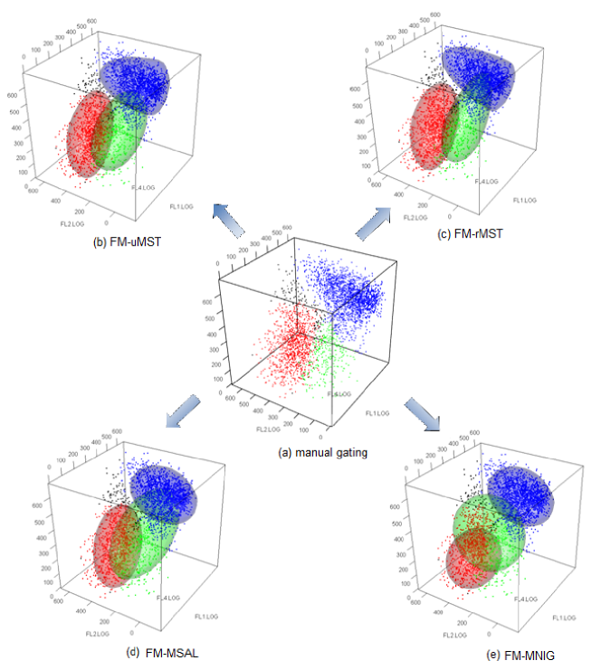
Figure 1: DLBCL dataset: Automated gating results of DLBCL sample using four different finite mixture models. The population of 3290 cells were stained with three fluorescence reagents - CD3 (FL1.LOG), CD5 (FL2.LOG), CD19 (FL4.LOG). (a) manual expert clustering of the DLBCL into three groups; (b) the fitted component contours of the three-component FM-uMST model; (c) the contours of the component densities of the fitted restricted (FM-rMST) model using EMMIX-skew; (d) the fitted component contours of the FM-MSAL model; (e) the contour plot of the fitted FM-MNIG model.

5 Concluding Remarks

We have presented a schematic way to classify multivariate skew distributions into four types, namely, the ‘restricted’, ‘unrestricted’, ‘extended’ and ‘generalized’ forms. Concerning the use of the terminology ‘restricted’ and ‘unrestricted’, it should be noted that the restricted skew forms are not nested within the corresponding unrestricted forms, with these two forms coinciding in the univariate case. However, these two forms are both special cases of the extended form, which itself is a special case of the generalized form.

Current work on finite mixtures of skew distributions has investigated only the restricted and unrestricted forms of multivariate skew distributions. Mixtures based on skew distributions of more general forms would be of interest for further research.

References

• Arellano-Valle and Azzalini (2006) Arellano-Valle RB, Azzalini A (2006) On the unification of families of skew-normal distributions. Scandinavian Journal of Statistics 33:561–574
• Arellano-Valle and Genton (2005) Arellano-Valle RB, Genton MG (2005) On fundamental skew distributions. Journal of Multivariate Analysis 96:93–116
• Arellano-Valle and Genton (2010) Arellano-Valle RB, Genton MG (2010) Multivariate extended skew-$t$ distributions and related families. METRON 68:201–234
• Arellano-Valle et al. (2006) Arellano-Valle RB, Branco MD, Genton MG (2006) A unified view on skewed distributions arising from selections. The Canadian Journal of Statistics 34:581–601
• Arellano-Valle et al. (2008) Arellano-Valle RB, Castro LM, Genton MG, Gómez HW (2008) Bayesian inference for shape mixtures of skewed distributions, with application to regression analysis. Bayesian Analysis 3:513–540
• Arnold et al. (1993) Arnold BC, Beaver RJ, Meeker WQ (1993) The nontruncated marginal of a truncated bivariate normal distribution. Psychometrika 58:471–478
• Azzalini (1985) Azzalini A (1985) A class of distributions which includes the normal ones. Scandinavian Journal of Statistics 12:171–178
• Azzalini (2005) Azzalini A (2005) The skew-normal distribution and related multivariate families. Scandinavian Journal of Statistics 32:159–188