Estimation and testing for partially linear single-index models

Abstract

In partially linear single-index models, we obtain the semiparametrically efficient profile least-squares estimators of regression coefficients. We also employ the smoothly clipped absolute deviation penalty (SCAD) approach to simultaneously select variables and estimate regression coefficients. We show that the resulting SCAD estimators are consistent and possess the oracle property. Subsequently, we demonstrate that a proposed tuning parameter selector, BIC, identifies the true model consistently. Finally, we develop a linear hypothesis test for the parametric coefficients and a goodness-of-fit test for the nonparametric component, respectively. Monte Carlo studies are also presented.

, , and t1Supported in part by NIH/NIAID Grant AI59773 and NSF Grant DMS-08-06097. t2Supported in part by the Merck Quantitative Sciences Fellowship Program. t3Supported by National Science Foundation Grants DMS-03-48869 and NIDA, NIH Grants R21 DA024260 and P50 DA10075. The content is solely the responsibility of the authors and does not necessarily represent the official views of the NIDA or the NIH.

1 Introduction

Regression analysis is commonly used to explore the relationship between a response variable $Y$ and its covariates $Z$. For the sake of convenience, one often employs a linear regression model $E(Y|Z)=Z^{\mathrm{T}}{\bolds{\alpha}}$ to assess the impact of the covariates on the response, where ${\bolds{\alpha}}$ is an unknown vector and $E$ stands for “expectation.” In practice, however, the linear assumption may not be valid. Hence, it is natural to consider a single-index model $E(Y|Z)=\eta(Z^{{\mathrm{T}}}{\bolds{\alpha}})$, in which the link function $\eta$ is unknown. Accordingly, various parameter estimators of single-index models have been proposed [e.g., Powell, Stock and Stocker (1989); Duan and Li (1991); Härdle, Hall and Ichimura (1993); Ichimura (1993); Horowitz and Härdle (1996); Liang and Wang (2005)]. Detailed discussion and illustration of the usefulness of this model can be found in Horowitz (1998). Although the single-index model plays an important role in data analysis, it may not be sufficient to explain the variation of responses via covariates $Z$. Therefore, Carroll et al. (1997) augmented the single-index model in a linear form with additional covariates $X$, which yields a partially linear single-index model (PLSIM), $E(Y|Z,X)=\eta(Z^{{\mathrm{T}}}{\bolds{\alpha}})+X^{{\mathrm{T}}}{\bolds{\beta}}$. When $Z$ is scalar and ${\bolds{\alpha}}=1$, the PLSIM reduces to the partially linear model, $E(Y|Z,X)=\eta(Z)+X^{{\mathrm{T}}}{\bolds{\beta}}$ [see Speckman (1988)]. A comprehensive review of partially linear models can be found in Härdle, Liang and Gao (2000).

To estimate parameters in partially linear single-index models, Carroll et al. (1997) proposed the backfitting algorithm. However, the resulting estimators may be unstable [see Yu and Ruppert (2002)] and undersmoothing the nonparametric function is necessary to reduce the bias of the parametric estimators. Accordingly, Yu and Ruppert (2002) proposed the penalized spline estimation procedure, while Xia and Härdle (2006) applied the minimum average variance estimation (MAVE) method, which was originally introduced by Xia et al. (2002) for dimension reduction. Although Yu and Ruppert’s procedure is useful, it may not yield efficient estimators; that is, the asymptotic covariance of their estimators does not reach the semiparametric efficiency bound [Carroll et al. (1997)]. In addition, these estimators need to be solved via an iterative procedure; that is, iteratively estimating the nonparametric component and the parametric component. We therefore propose the profile least-squares approach, which obtains efficient estimators and provides the efficient bound. Moreover, the resulting estimators can be found without using the iterative procedure mentioned above and hence may reduce the computational burden.

In data analysis, the true model is often unknown; this allows the possibility of selecting an underfitted (or overfitted) model, leading to biased (or inefficient) estimators and predictions. To address this problem, Tibshirani (1996) introduced the least absolute shrinkage and selection operator (LASSO) to shrink the estimated coefficients of superfluous variables to zero in linear regression models. Subsequently, Fan and Li (2001) proposed the smoothly clipped absolute deviation (SCAD) approach that not only selects important variables consistently, but also produces parameter estimators as efficiently as if the true model were known, a property not possessed by the LASSO. Because it is not a simple matter to formulate the penalized function via the MAVE’s procedure, we employ the profile least-squares approach to obtain the SCAD estimators for both parameter vectors ${\bolds{\alpha}}$ and ${\bolds{\beta}}$. Furthermore, we establish the asymptotic results of the SCAD estimators, which include the consistency and oracle properties [see Fan and Li (2001)]. Simulation results are consistent with theoretical findings.

After estimating unknown parameters, it is natural to construct hypothesis tests to assess the appropriateness of the linear constraint hypothesis as well as the linearity of the nonparametric function. We demonstrate that the resulting test statistics are asymptotically chi-square distributed under the null hypothesis. In addition, simulation studies indicate that the test statistics perform well. The rest of this paper is organized as follows. Section 2 introduces the profile least-squares estimators and the penalized SCAD estimators. The asymptotic properties of these estimators are obtained. Section 3 presents hypothesis tests and their large-sample properties. Monte Carlo studies are presented in Section 4. Section 5 concludes the article with a brief discussion. All detailed proofs are deferred to the Appendix.

2 Profile least-squares procedure

Suppose that $\{(Y_{i},Z_{i},X_{i}),i=1,\ldots,n\}$ is a random sample generated from the PLSIM

$$Y=\eta(Z^{{\mathrm{T}}}{\bolds{\alpha}})+X^{{\mathrm{T}}}{\bolds{\beta}}+\varepsilon,$$ (1)

where $Z$ and $X$ are $p$-dimensional and $q$-dimensional covariate vectors, respectively, ${\bolds{\alpha}}=(\alpha_{1},\ldots,\alpha_{p})^{{\mathrm{T}}}$, ${\bolds{\beta}}=(\beta_{1},\ldots,\beta_{q})^{{\mathrm{T}}}$, $\eta(\cdot)$ is an unknown differentiable function, $\varepsilon$ is the random error with mean zero and finite variance $\sigma^{2}$, and $(Z^{{\mathrm{T}}},X^{{\mathrm{T}}})^{{\mathrm{T}}}$ and $\varepsilon$ are independent. Furthermore, we assume that $\|{\bolds{\alpha}}\|=1$ and that the first element of ${\bolds{\alpha}}$ is positive, to ensure identifiability. We then employ the profile least-squares procedure to obtain efficient estimators and SCAD estimators in the following two subsections, respectively.

2.1 Profile least-squares estimator

In semiparametric models, Severini and Wong (1992) applied the profile likelihood approach to estimate the parametric component. We adapt this approach to estimate unknown parameters of partially linear single-index models. To begin, we re-express model (1) as

$$Y_{i}^{*}=\eta(\Lambda_{i})+\varepsilon_{i},$$

where $Y^{*}_{i}=Y_{i}-X_{i}^{\mathrm{T}}{\bolds{\beta}}$ and $\Lambda_{i}=Z_{i}^{\mathrm{T}}{\bolds{\alpha}}$. Then, for a given ${\bolds{\zeta}}=({\bolds{\alpha}}^{\mathrm{T}},{\bolds{\beta}}^{\mathrm{T}})^{\mathrm{T}}$, we employ the local linear regression technique [Fan and Gijbels (1996)] to estimate $\eta$, that is, to minimize

$$\sum_{i=1}^{n}\{a+b(\Lambda_{i}-u)+X_{i}^{\mathrm{T}}{\bolds{\beta}}-Y_{i}\}^{2}K_{h}(\Lambda_{i}-u)$$ (2)

with respect to $a$, $b$, where $K_{h}(\cdot)=1/hK(\cdot/h)$, $K(\cdot)$ is a kernel function and $h$ is a bandwidth.

Let $(\hat{a},\hat{b})$ be the minimizer of (2). Then,

$$\hat{\eta}(u,{\bolds{\zeta}})=\hat{a}=\frac{K_{20}(u,{\bolds{\zeta}})K_{01}(u,{\bolds{\zeta}})-K_{10}(u,{\bolds{\zeta}})K_{11}(u,{\bolds{\zeta}})}{K_{00}(u,{\bolds{\zeta}})K_{20}(u,{\bolds{\zeta}})-K_{10}^{2}(u,{\bolds{\zeta}})},$$ (3)

where $K_{jl}(u,{\bolds{\zeta}})=\sum_{i=1}^{n}K_{h}(Z_{i}^{{\mathrm{T}}}{\bolds{\alpha}}-u)(Z_{i}^{{\mathrm{T}}}{\bolds{\alpha}}-u)^{j}(X_{i}^{{\mathrm{T}}}{\bolds{\beta}}-Y_{i})^{l}$ for $j=0,1,2$ and $l=0,1$. Subsequently, following Jennrich’s (1969) assumption (a), there exists a profile least-squares estimator $\hat{{\bolds{\zeta}}}=(\hat{{\bolds{\alpha}}}{}^{{\mathrm{T}}},\hat{{\bolds{\beta}}}{}^{{\mathrm{T}}})^{{\mathrm{T}}}$ obtained by minimizing the following profile least-squares function:

$$Q({\bolds{\zeta}})=\sum_{i=1}^{n}\{Y_{i}-\hat{\eta}(Z_{i}^{{\mathrm{T}}}{\bolds{\alpha}},{\bolds{\zeta}})-X_{i}^{{\mathrm{T}}}{\bolds{\beta}}\}^{2}.$$ (4)

It is noteworthy that we apply the Newton–Raphson iterative method to find the estimator $\hat{{\bolds{\zeta}}}$; this technique is distinct from the more commonly used iterative procedure in partially single-index models which iteratively updates estimates of the nonparametric component and the parametric component obtained from their corresponding objective functions. In addition, our proposed profile least-squares approach allows us to directly introduce the penalized function, as given in the next subsection.

To study the large-sample properties of parameter estimators, we consider the true model with an unknown parameter vector ${\bolds{\zeta}}_{0}=({\bolds{\alpha}}_{0}^{\mathrm{T}},{\bolds{\beta}}_{0}^{\mathrm{T}})^{\mathrm{T}}$. In addition, we assume that ${\bolds{\alpha}}_{0}^{\mathrm{T}}$ and ${\bolds{\beta}}_{0}^{\mathrm{T}}$ have the same dimensions as their corresponding parameter vectors ${\bolds{\alpha}}^{\mathrm{T}}$ and ${\bolds{\beta}}^{\mathrm{T}}$ in the candidate model of this subsection. Moreover, we introduce the following notation: $A^{\otimes 2}=AA^{\mathrm{T}}$ for a matrix $A$, $\Lambda=Z^{{\mathrm{T}}}{\bolds{\alpha}}$, $\hat{\Lambda}=Z^{{\mathrm{T}}}\hat{{\bolds{\alpha}}}$, $\Lambda_{0}=Z^{\mathrm{T}}{\bolds{\alpha}}_{0}$, $\widetilde{\xi}=\xi-E(\xi|\Lambda)$, $\widetilde{\xi}_{0}=\xi-E(\xi|\Lambda_{0})$ and $\hat{\xi}=\xi-\hat{E}(\xi|\Lambda)$ for any random variable (or vector) $\xi$, where $\hat{E}(\xi|\Lambda)$ is the local linear estimator of $E(\xi|\Lambda)$. For example, $\widetilde{Z}=Z-E(Z|\Lambda)$ and $\hat{X}=X-\hat{E}(X|\Lambda)$. We next present six conditions and then obtain the weak consistency and asymptotic normality of the profile least-squares estimators.

The function $\eta(\cdot)$ is differentiable and not constant on the support ${\mathcal{U}}$ of $Z^{\mathrm{T}}{\bolds{\alpha}}$.

The function $\eta(z^{\mathrm{T}}{\bolds{\alpha}})$ and the density function of $Z^{{\mathrm{T}}}{\bolds{\alpha}}$, $f_{{\bolds{\alpha}}}(z)$, are both three times continuously differentiable with respect to $z$. The third derivatives are uniformly Lipschitz continuous over ${\mathcal{A}}\subset{\mathcal{R}}^{p}$ for all $u\in\{u=z^{\mathrm{T}}{\bolds{\alpha}}\dvtx{\bolds{\alpha}}\in{\mathcal{A}},z\in{\mathcal{Z}}\subset{\mathcal{R}}^{p}\}$.

$E(|Y|^{m_{1}})<\infty$ for some $m_{1}\geq 3$. The conditional variance of $Y$ given $(X,Z)$ is bounded and bounded away from $0$.

The kernel function $K(\cdot)$ is twice continuously differentiable with the support $(-1,1)$. In addition, its second derivative is Lipschitz continuous. Moreover, $\int u^{j}K(u)\,du=1$ if $j=0$ and $=0$ if $j=1$.

The bandwidth $h$ satisfies $\{nh^{3+3/{(m_{1}-1)}}\}\log^{-1}n\to\infty$ and $nh^{8}\to 0$ as $n\to\infty$.

$E(\widetilde{X}^{\otimes 2})$ and $E\{\widetilde{Z}\eta^{\prime}(\Lambda)\}^{\otimes 2}$ are positive-definite, where $\eta^{\prime}$ is the first derivative of $\eta$.

Theorem 1

Under the regularity conditions (i)–(vi), with probability tending to one, $\hat{{\bolds{\zeta}}}$ is a consistent estimator of ${\bolds{\zeta}}$. Furthermore, $\sqrt{n}(\hat{{\bolds{\zeta}}}-{\bolds{\zeta}}_{0})\to N(0,\sigma^{2}\mathbf{D}^{-1})$ in distribution, where $\mathbf{D}=E[\{\eta^{\prime}(\Lambda_{0})\widetilde{Z}_{0}^{\mathrm{T}},\widetilde{X}_{0}^{{\mathrm{T}}}\}^{{\mathrm{T}}}]^{\otimes 2}$. Moreover, $\hat{{\bolds{\zeta}}}$ is a semiparametrically efficient estimator.

Because $(Z^{{\mathrm{T}}},X^{{\mathrm{T}}})^{{\mathrm{T}}}$ is independent of $\varepsilon$, we are able to demonstrate that the asymptotic variance of Xia and Härdle’s (2006) minimum average variance estimator is $\sigma^{2}\mathbf{D}^{-1}$, which indicates that MAVE is also an efficient estimator.

After having estimated ${\bolds{\alpha}}$ and ${\bolds{\beta}}$, we obtain the following estimator of $\eta(u)$:

$$\hat{\eta}(u)=\hat{\eta}(u,\hat{{\bolds{\zeta}}})=\frac{K_{20}(u,\hat{{\bolds{\zeta}}})K_{01}(u,\hat{{\bolds{\zeta}}})-K_{10}(u,\hat{{\bolds{\zeta}}})K_{11}(u,\hat{{\bolds{\zeta}}})}{K_{00}(u,\hat{{\bolds{\zeta}}})K_{20}(u,\hat{{\bolds{\zeta}}})-K_{10}^{2}(u,\hat{{\bolds{\zeta}}})}.$$

If the density function $f_{\Lambda_{0}}$ of $\Lambda_{0}$ is positive and the derivative of $E(\varepsilon^{2}|\Lambda_{0}=u)$ exists, then we can further demonstrate that $(nh)^{1/2}\{\hat{\eta}(u)-\eta(u)-1/\break 2k_{2}\eta^{\prime\prime}(u)h^{2}\}$ converges to a normal distribution $N(0,\sigma_{\eta,u}^{2})$, where $\sigma_{\eta,u}^{2}=f^{-1}_{\Lambda_{0}}(u)\int K^{2}(t)\,dt\times E(\varepsilon^{2}|\Lambda_{0}=u)$, $k_{2}=\int K(t)t^{2}\,dt$ and $\eta^{\prime\prime}$ is the second derivative of $\eta$. It is also noteworthy that one usually either introduces a trimming function or adds a ridge parameter [see Seifert and Gassert (1996)] when the denominator of $\hat{\eta}$ closes to zero.

Remark 1.

Condition (v) indicates that Theorem 1 is applicable for a reasonable range of bandwidths. Numerical studies confirm it; our results remain stable by employing various bandwidths around the optimal bandwidth selected by cross-validation, in particular when the sample size becomes large.

2.2 Penalized profile least-squares estimator

In practice, the true model is often unknown a priori. An underfitted model can yield biased estimates and predicted values, while an overfitted model can degrade the efficiency of the parameter estimates and predictions. This motivates us to apply the penalized least-squares approach to simultaneously estimate parameters and select important variables. To this end, we consider a penalized profile least-squares function

$${\mathcal{L}}_{P}({\bolds{\zeta}})=\frac{1}{2}Q({\bolds{\zeta}})+n\sum_{j=1}^{p}p_{\lambda_{1j}}(|\alpha_{j}|)+n\sum_{k=1}^{q}p_{\lambda_{2k}}(|\beta_{k}|),$$ (5)

where $p_{\lambda}(\cdot)$ is a penalty function with a regularization parameter $\lambda$. Throughout this paper, we allow different elements of ${\bolds{\alpha}}$ and ${\bolds{\beta}}$ to have different penalty functions with different regularization parameters. For the purpose of selecting $X$-variables only, we simply set $p_{\lambda_{1j}}(\cdot)=0$ and the resulting penalized profile least-squares function becomes

$${\mathcal{L}}_{P}({\bolds{\zeta}})=\frac{1}{2}Q({\bolds{\zeta}})+n\sum_{k=1}^{q}p_{\lambda_{2k}}(|\beta_{j}|).$$ (6)

Similarly, if we are only interested in selecting $Z$-variables, then we set $p_{\lambda_{2k}}(\cdot)=0$ so that

$${\mathcal{L}}_{P}({\bolds{\zeta}})=\frac{1}{2}Q({\bolds{\zeta}})+n\sum_{j=1}^{p}p_{\lambda_{1j}}(|\alpha_{j}|).$$ (7)

There are various penalty functions available in the literature. To obtain the oracle property of Fan and Li (2001), we adopt their SCAD penalty, whose first derivative is

$$p_{\lambda}^{\prime}(\theta)=\lambda\biggl{\{}I(\theta\leq\lambda)+\frac{(a\lambda-\theta)_{+}}{(a-1)\lambda}I(\theta>\lambda)\biggr{\}},$$

and where $p_{\lambda}(0)=0$, $a=3.7$ and $(t)_{+}=tI\{t>0\}$ is the hinge loss function. For the given tuning parameters, we obtain the penalized estimators by minimizing ${\mathcal{L}}_{P}({\bolds{\alpha}},{\bolds{\beta}})$ with respect to ${\bolds{\alpha}}$ and ${\bolds{\beta}}$. For the sake of simplicity, we denote the resulting estimators by $\hat{{\bolds{\alpha}}}_{\lambda_{1}}$ and $\hat{{\bolds{\beta}}}_{\lambda_{2}}$.

In what follows, we study the theoretical properties of the penalized profile least-squares estimators with the SCAD penalty. Without loss of generality, it is assumed that the correct model has regression coefficients ${\bolds{\alpha}}_{0}=({\bolds{\alpha}}_{10}^{{\mathrm{T}}},{\bolds{\alpha}}_{20}^{{\mathrm{T}}})^{{\mathrm{T}}}$ and ${\bolds{\beta}}_{0}=({\bolds{\beta}}_{10}^{\mathrm{T}},{\bolds{\beta}}_{20}^{{\mathrm{T}}})^{{\mathrm{T}}}$, where ${\bolds{\alpha}}_{10}$ and ${\bolds{\beta}}_{10}$ are $p_{0}\times 1$ and $q_{0}\times 1$ nonzero components of ${\bolds{\alpha}}_{0}$ and ${\bolds{\beta}}_{0}$, respectively, and ${\bolds{\alpha}}_{20}$ and ${\bolds{\beta}}_{20}$ are $(p-p_{0})\times 1$ and $(q-q_{0})\times 1$ vectors with zeros. In addition, we define $Z_{1}$ and $X_{1}$ in such a way that they consist of the first $p_{0}$ and $q_{0}$ elements of $Z$ and $X$, respectively. We define $\widetilde{Z}_{1}$ and $\widetilde{X}_{1}$ analogously. Finally, we use the following notation for simplicity: $\Gamma_{\widetilde{X}_{1}\widetilde{X}_{1}}=E(\widetilde{X}_{1}^{\otimes 2})$, $\Gamma_{\widetilde{X}_{1}\widetilde{Z}_{1}}=E\{\widetilde{Z}_{1}\widetilde{X}_{1}^{\mathrm{T}}\eta^{\prime}(\Lambda)\}$ and $\Gamma_{\widetilde{Z}_{1}\widetilde{Z}_{1}}=E\{\widetilde{Z}_{1}\eta^{\prime}(\Lambda)\}^{\otimes 2}$.

Theorem 2

Under the regularity conditions (i)–(vi), if, for all $k$ and $j$, $\lambda_{1j}\to 0$, $\sqrt{n}\lambda_{1j}\to\infty$, $\lambda_{2k}\to 0$ and $\sqrt{n}\lambda_{2k}\to\infty$ as $n\to\infty$, with probability tending to one, then the penalized estimators $\hat{{\bolds{\alpha}}}_{\lambda_{1}}=(\hat{{\bolds{\alpha}}}_{1{\lambda_{1}}}^{\mathrm{T}},\hat{{\bolds{\alpha}}}_{2{\lambda_{1}}}^{\mathrm{T}})^{\mathrm{T}}$ and $\hat{{\bolds{\beta}}}_{\lambda_{2}}=(\hat{{\bolds{\beta}}}{}^{\mathrm{T}}_{1{\lambda_{2}}},\hat{{\bolds{\beta}}}{}^{\mathrm{T}}_{2{\lambda_{2}}})^{\mathrm{T}}$ satisfy:

$\hat{{\bolds{\alpha}}}_{2{\lambda_{1}}}=0$ and $\hat{{\bolds{\beta}}}_{2{\lambda_{2}}}=0$;

$\sqrt{n}(\hat{{\bolds{\alpha}}}_{1{\lambda_{1}}}-{\bolds{\alpha}}_{10})\to N\{0,\sigma^{2}(\Gamma_{\widetilde{Z}_{1}\widetilde{Z}_{1}}-\Gamma_{\widetilde{X}_{1}\widetilde{Z}_{1}}\Gamma_{\widetilde{X}_{1}\widetilde{X}_{1}}^{-1}\Gamma_{\widetilde{X}_{1}\widetilde{Z}_{1}}^{\mathrm{T}})^{-1}\}$ and$\sqrt{n}(\hat{{\bolds{\beta}}}_{1{\lambda_{2}}}-{\bolds{\beta}}_{10})\to N\{0,\sigma^{2}(\Gamma_{\widetilde{X}_{1}\widetilde{X}_{1}}-\Gamma_{\widetilde{X}_{1}\widetilde{Z}_{1}}^{\mathrm{T}}\Gamma_{\widetilde{Z}_{1}\widetilde{Z}_{1}}^{-1}\Gamma_{\widetilde{X}_{1}\widetilde{Z}_{1}})^{-1}\}$.

Analogous results can be established for those parameter estimators obtained via the penalized functions (6) or (7).

Kong and Xia (2007) developed a cross-validation-based variable selection procedure in single-index models and observed the difference between the popular leave-$m$-out cross-validation method in the variable selection of the linear model and the single-index model. It is noteworthy that we need two tuning parameters in (5), $\lambda_{1}$ and $\lambda_{2}$, imposed on the linear part and the single-index part, respectively. They can be in the same order in the large-sample sense, on the basis of the assumptions in Theorem 2, although the distinction between these two tuning parameters in practice is anticipated, as will be discussed below. Theorem 2 indicates that the proposed variable selection procedure possesses the oracle property. However, this attractive feature relies on the tuning parameters. To this end, we adopt Wang, Li and Tsai’s (2007) BIC selector to choose the regularization parameters $\lambda_{1j}$ and $\lambda_{2k}$. Because it is computationally expensive to minimize BIC, defined below, with respect to the $(p+q)$-dimensional regularization parameters, we follow the approach of Fan and Li (2004) to set $\lambda_{1j}=\lambda\operatorname{SE}(\hat{\alpha}_{j}^{u})$ and $\lambda_{2k}=\lambda\operatorname{SE}(\hat{\beta}_{k}^{u})$, where $\lambda$ is the tuning parameter, and $\operatorname{SE}(\hat{\alpha}_{j}^{u})$ and $\operatorname{SE}(\hat{\beta}_{k}^{u})$ are the standard errors of the unpenalized profile least-squares estimators of $\alpha_{j}$ and $\beta_{k}$, respectively, for $j=1,\ldots,p$ and $k=1,\ldots,q$. Let the resulting SCAD estimators be $\hat{{\bolds{\alpha}}}_{\lambda}$ and $\hat{{\bolds{\beta}}}_{\lambda}$. We then select $\lambda$ by minimizing the objective function

$$\operatorname{BIC}(\lambda)=\log\{(\operatorname{MSE}(\lambda)\}+\bigl{(}\log(n)/n\bigr{)}\operatorname{DF}_{\lambda},$$ (8)

where $\operatorname{MSE}(\lambda)=n^{-1}\sum_{i=1}^{n}\{Y_{i}-\hat{\eta}(Z_{i}^{{\mathrm{T}}}\hat{{\bolds{\alpha}}}_{\lambda})-X_{i}^{{\mathrm{T}}}\hat{{\bolds{\beta}}}_{\lambda}\}^{2}$ and $\operatorname{DF}_{\lambda}$ is the number of nonzero coefficients of both $\hat{{\bolds{\alpha}}}_{\lambda}$ and $\hat{{\bolds{\beta}}}_{\lambda}$. More specifically, we choose $\lambda$ to be the minimizer among a set of grid points over bounded interval $[0,\lambda_{\mathrm{max}}]$, where $\lambda_{\mathrm{max}}/\sqrt{n}\to 0$ as $n\to\infty$. The resulting optimal tuning parameter is denoted by $\hat{\lambda}$. In practice, a plot of the BIC($\lambda$) against $\lambda$ can be used to determine an appropriate $\lambda_{\mathrm{max}}$ to ensure that the BIC$(\lambda)$ reaches its minimum around the middle of the range of $\lambda$. The grid points for $\lambda$ are then taken to be evenly distributed over $[0,\lambda_{\mathrm{max}}]$ so that they are chosen to be fine enough to avoid multiple minimizers of BIC($\lambda$). In our numerical studies, the range for $\lambda$ and the number of grid points are set in the same manner as those in Wang, Li and Tsai (2007) and Zhang, Li and Tsai (2010). Based on our limited experience, the resulting estimate of $\lambda$ is quite stable with respect to the number of grid points when they are sufficiently fine.

To investigate the theoretical properties of the BIC selector, we denote by $S=\{j_{1},\ldots,j_{d}\}$ the set of the indices of the covariates in the given candidate model, which contains indices of both $X$ and $Z$. In addition, let $S_{T}$ be the true model, $S_{F}$ be the full model and $S_{\lambda}$ be the set of the indices of the covariates selected by the SCAD procedure with tuning parameter $\lambda$. For a given candidate model $S$ with parameter vectors ${\bolds{\alpha}}_{s}$ and ${\bolds{\beta}}_{s}$, let $\hat{{\bolds{\alpha}}}_{s}$ and $\hat{{\bolds{\beta}}}_{s}$ be the corresponding profile least-squares estimators. Then, define $\sigma_{n}^{2}(S)=n^{-1}\sum_{i=1}^{n}\{Y_{i}-\hat{\eta}(Z_{i}^{{\mathrm{T}}}\hat{{\bolds{\alpha}}}_{s})-X_{i}^{{\mathrm{T}}}\hat{{\bolds{\beta}}}_{s}\}^{2}$ and further assume that:

1. for any $S\subset S_{F}$, $\sigma_{n}^{2}(S)\to\sigma^{2}(S)$ in probability for some $\sigma^{2}(S)>0$;

2. for any $S\not\supset S_{T}$, we have $\sigma^{2}(S)>\sigma^{2}(S_{T})$.

It is noteworthy that (A) and (B) are the standard conditions for investigating parameter estimation under model misspecification [e.g., see Wang, Li and Tsai (2007)].

We next present the asymptotic property of the BIC-type tuning parameter selector.

Theorem 3

Under conditions (A), (B) and the regularity conditions (i)–(vi), we have

$$P(S_{\widehat{\lambda}}=S_{T})\to 1.\vspace*{-2pt}$$ (9)

Theorem 3 demonstrates that the BIC tuning parameter selector enables us to select the true model consistently.

3 Hypothesis tests

Applying the estimation method described in the previous section, we propose two hypothesis tests. The first is for general hypothesis testing of regression parameters and the second is for testing the nonparametric function.

3.1 Testing parametric components

Consider the general linear hypothesis

$$H_{0}\dvtx\mathbf{A}{\bolds{\zeta}}={\bolds{\delta}}\quad\mbox{versus}\quad H_{1}\dvtx\mathbf{A}{\bolds{\zeta}}\neq{\bolds{\delta}},$$ (10)

where $\mathbf{A}$ is a known $m\times(p+q)$ full-rank matrix and ${\bolds{\delta}}$ is an $m\times 1$ vector. A simple example of (10) is to test whether some elements of ${\bolds{\alpha}}$ and ${\bolds{\beta}}$ are zero; that is,

$$H_{0}\dvtx\alpha_{i_{1}}=\cdots=\alpha_{i_{k}}=0\mbox{ and }\beta_{j_{1}}=\cdots=\beta_{j_{l}}=0$$

versus

$$H_{1}\dvtx\mbox{not all }\alpha_{i_{1}},\ldots,\alpha_{i_{k}}\mbox{ and }\beta_{j_{1}},\ldots,\beta_{j_{l}}\mbox{ are equal to }0.$$

Under $H_{0}$ and $H_{1}$, let ${\bolds{\zeta}}_{0}=({\bolds{\alpha}}_{0}^{\mathrm{T}},{\bolds{\beta}}_{0}^{\mathrm{T}})^{\mathrm{T}}$ and ${\bolds{\zeta}}_{1}=({\bolds{\alpha}}_{1}^{\mathrm{T}},{\bolds{\beta}}_{1}^{\mathrm{T}})^{\mathrm{T}}$ be the corresponding parameter vectors, and let $\Omega_{0}$ and $\Omega_{1}$ be the parameter spaces of ${\bolds{\zeta}}_{0}$ and ${\bolds{\zeta}}_{1}$, respectively. It is noteworthy that this is a slight abuse of notation because ${\bolds{\zeta}}_{0}$ was previously used to denote the true value of ${\bolds{\zeta}}$ in Section 2.1. Furthermore, define

$$Q(H_{0})=\inf_{\Omega_{0}}Q({\bolds{\zeta}}_{0})=\sum^{n}_{i=1}\{Y_{i}-{\mathbf{X}}_{i}^{\mathrm{T}}\hat{{\bolds{\beta}}}_{0}-\hat{\eta}(Z_{i}^{{\mathrm{T}}}\hat{{\bolds{\alpha}}}_{0},\hat{\bolds{\zeta}}_{0})\}^{2}$$

and

$$Q(H_{1})=\inf_{\Omega_{1}}Q({\bolds{\zeta}}_{1})=\sum^{n}_{i=1}\{Y_{i}-{\mathbf{X}}_{i}^{\mathrm{T}}\hat{{\bolds{\beta}}}_{1}-\hat{\eta}(Z_{i}^{{\mathrm{T}}}\hat{\bolds{\alpha}}_{1},\hat{\bolds{\zeta}}_{1})\}^{2},$$

where $\{\hat{{\bolds{\beta}}}_{0},\hat{\bolds{\zeta}}_{0}\}$ and $\{\hat{{\bolds{\beta}}}_{1},\hat{\bolds{\zeta}}_{1}\}$ are the profile least-squares estimators of $\{{\bolds{\beta}}_{0},{\bolds{\zeta}}_{0}\}$ and $\{{\bolds{\beta}}_{1},{\bolds{\zeta}}_{1}\}$, respectively, and $\hat{\eta}$ is the nonparametric estimator of $\eta$ obtained via (3). Subsequently, we propose a test statistic,

$$T_{1}=\frac{n\{Q(H_{0})-Q(H_{1})\}}{Q(H_{1})},$$

and give its theoretical property below.

Theorem 4

Assume that the regularity conditions (i)–(vi) hold. Then:

under $H_{0}$ in (10), $T_{1}\rightarrow\chi_{m}^{2};$

under $H_{1}$ in (10), $T_{1}$ converges to a noncentral chi-squared distribution with $m$ degrees of freedom and noncentrality parameter $\phi=\break\lim_{n\to\infty}n\sigma^{-2}(\mathbf{A}{\bolds{\zeta}}-{\bolds{\delta}})^{\mathrm{T}}(\mathbf{A}\mathbf{D}^{-1}\mathbf{A}^{\mathrm{T}})^{-1}(\mathbf{A}{\bolds{\zeta}}-{\bolds{\delta}})$, where $\mathbf{D}$ is defined as in Theorem 1.

Analogously, we are able to construct the Wald test, $W_{n}=(\mathbf{A}\hat{{\bolds{\zeta}}}-\break{\bolds{\delta}})^{\mathrm{T}}(\mathbf{A}\hat{\mathbf{D}}^{-1}\times\mathbf{A}^{\mathrm{T}})^{-1}(\mathbf{A}\hat{{\bolds{\zeta}}}-{\bolds{\delta}})$, and demonstrate that $W_{n}$ and $T_{1}$ have the same asymptotic distribution.

3.2 Testing the nonparametric component

The nonparametric estimate of $\eta(\cdot)$ provides us with descriptive and graphical information for exploratory data analysis. Using this information, it is possible to formulate a parametric model that takes into account the features that emerged from the preliminary analysis. To this end, we introduce a goodness-of-fit test to assess the appropriateness of a proposed parametric model. Without loss of generality, we consider a simple linear model under the null hypothesis. Accordingly, the null and alternative hypotheses are given as follows:

$$\hskip 20.0ptH_{0}\dvtx\eta(u)=\theta_{0}+\theta_{1}u\quad\mbox{versus}\quad H_{1}\dvtx\eta(u)\neq\theta_{0}+\theta_{1}u\qquad\mbox{for some }u,$$

where $\theta_{0}$ and $\theta_{1}$ are unknown constant parameters.

Under $H_{1}$, let $\hat{\bolds{\alpha}}$, $\hat{{\bolds{\beta}}}$ and $\hat{\eta}$ be the corresponding profile least-squares and nonparametric estimators of ${\bolds{\alpha}}$, ${\bolds{\beta}}$ and $\eta$, respectively. Under $H_{0}$, we use the same parametric estimators $\hat{\bolds{\alpha}}$ and $\hat{{\bolds{\beta}}}$ as those obtained under $H_{1}$, while the estimator of $\eta$ is $\tilde{\eta}(u)=\hat{\theta}_{0}+\hat{\theta}_{1}u$, where $\hat{\theta}_{0}$ and $\hat{\theta}_{1}$ are the ordinary least-squares estimators of $\theta_{0}$ and $\theta_{1}$, respectively, by fitting $Y_{i}-X_{i}^{\mathrm{T}}\hat{\bolds{\beta}}$ versus $Z_{i}^{\mathrm{T}}\hat{\bolds{\alpha}}$. The resulting residual sums of squares under the null and alternative hypotheses are then

$$\operatorname{RSS}(H_{0})=\sum_{i=1}^{n}\{Y_{i}-\tilde{\eta}(Z_{i}^{\mathrm{T}}\hat{\bolds{\alpha}})-X_{i}^{\mathrm{T}}\hat{\bolds{\beta}}\}^{2}$$

and

$$\operatorname{RSS}(H_{1})=\sum_{i=1}^{n}\{Y_{i}-\hat{\eta}(Z_{i}^{\mathrm{T}}\hat{\bolds{\alpha}})-X_{i}^{\mathrm{T}}\hat{\bolds{\beta}}\}^{2}.$$

To test the null hypothesis, we consider the following generalized $F$-test:

$$T_{2}=\frac{r_{K}}{2}\frac{n\{\operatorname{RSS}(H_{0})-\operatorname{RSS}(H_{1})\}}{\operatorname{RSS}(H_{1})},$$

where $r_{K}=\{K(0)-0.5\int K^{2}(u)\,du\}\{\int\{K(u)-0.5K*K(u)\}\,du\}^{-1}$ and $K*K$ denotes the convolution of $K$. The theoretical property of $T_{2}$ is given below.

Theorem 5

Assume that the regularity conditions (i)–(vi) hold. Under $H_{0}$ in (3.2), $T_{2}$ has an asymptotic $\chi^{2}$ distribution with $df_{n}$ degrees of freedom, where $df_{n}=r_{K}|{\mathcal{U}}|\{K(0)-0.5\int K^{2}(u)\,du\}/h$, $|{\mathcal{U}}|$ stands for the length of ${\mathcal{U}}$ and $\mathcal{U}$ is defined in regularity condition (i).

The above theorem unveils the Wilks phenomenon for the partially linear single-index model. Furthermore, we can obtain an analogous result when the simple linear model under $H_{0}$ is replaced by a multiple regression model.

4 Simulation studies

In this section, we present four Monte Carlo studies which evaluate the finite-sample performance of the proposed estimation and testing methods. The first two examples illustrate the performance of the profile least-squares estimator and the SCAD-based variable selection procedure proposed in Sections 2.1 and 2.2, respectively. The next two examples explore the performance of the test statistics developed in Sections 3.1 and 3.2.

Example 4.1.

We generated $500$ realizations, each consisting of $n=50,100$ and $200$ observations, from each of the following models:

$$y = 4\bigl{\{}(z_{1}+z_{2}-1)/{\sqrt{2}}\bigr{\}}^{2}+4+0.2\varepsilon;$$ (11)

$$y = \sin\bigl{[}\bigl{\{}(z_{1}+z_{2}+z_{3})/{\sqrt{3}}-a\bigr{\}}\pi/(b-a)\bigr{]}+\beta X+0.1\varepsilon,$$ (12)

where $z_{1},z_{2},z_{3}$ are independent and uniformly distributed on $[0,1]$, $X=0$ for the odd numbered observations and $X=1$ for the even numbered observations, $\varepsilon$ has the standard normal distribution, $a=0.3912$ and $b=1.3409$. The resulting parameters of models (11) and (12) are ${\bolds{\alpha}}=(\alpha_{1},\alpha_{2})^{{\mathrm{T}}}=(0.7071,0.7071)^{{\mathrm{T}}}$ and $({\bolds{\alpha}},\beta)=(\alpha_{1},\alpha_{2},\alpha_{3},\beta)^{{\mathrm{T}}}=(0.5774,0.5774,0.5774,0.3)^{{\mathrm{T}}}$ with $\phi_{0}=\arccos(\alpha_{1})=0.7854$ as in Xia and Härdle (2006) [or $\pi/4$ in Härdle, Hall and Ichimura (1993), page 165].

Model (11) was analyzed by Härdle, Hall and Ichimura (1993) and Xia and Härdle (2006), while model (12) was investigated by Carroll et al. (1997) and Xia and Härdle (2006). For both models, Xia and Härdle claimed that their MAVE approach outperforms those of Härdle, Hall and Ichimura (1993) and Carroll et al. (1997), respectively. It is therefore of interest to compare the profile least-squares (abbreviated to PrLS) method with MAVE. Tables 1 and 2 present the results for models (11) and (12), respectively. Both tables indicate that the profile least-squares method yields accurate estimates and that the mean squared error becomes smaller as the sample size gets larger, which is consistent with the theoretical finding. Furthermore, Table 1 shows that the mean squared errors of $\hat{\bolds{\alpha}}$ and $\hat{\bolds{\beta}}$ are smaller than those computed via the MAVE method [see Table 1 of Xia and Härdle (2006)]. Table 2 suggests that the biases and their associated mean squared errors of $\hat{\bolds{\alpha}}$ and $\hat{\bolds{\beta}}$ are comparable to those calculated via MAVE. In summary, the Monte Carlo studies indicate that PrLS performs well. Because the penalized MAVE is not easy to obtain, we study only the penalized PrLS estimates in the following example.

=310pt $\bolds{n}$ $\bolds{\alpha_{1}\,(=0.7071)}$ $\bolds{\alpha_{2}\,(=0.7071)}$ $\bolds{\phi_{0}\,(=0.7854)}$ 50 00.7053 (21.5274) 00.7059 (21.3398) 0.7859 (42.9158) 100 0.7054 (8.5874) 0.7076 (8.4175) 0.7869 (17.0116) 200 0.7067 (4.4636) 0.7069 (4.4287) 0.7856 (8.8942)0

Table 1: Simulation results for Example 4.1: the profile least-squares estimates (PrLS) and their corresponding mean squared errors ($\times 10^{-4}$) for model (11)

=315pt $\bolds{n}$ $\bolds{\alpha_{1}\,(=0.5774)}$ $\bolds{\alpha_{2}\,(=0.5774)}$ $\bolds{\alpha_{3}\,(=0.5774)}$ $\bolds{\beta\,(=0.3)}$ 50 0.5753 (5.8336) 0.5771 (5.5685) 0.5782 (5.9245) 00.2923 (11.4582) 100 0.5776 (2.5009) 0.5774 (2.4606) 0.5764 (2.4770) 0.3000 (4.7030) 200 0.5782 (1.1533) 0.5771 (1.0852) 0.5764 (1.2483) 0.3004 (2.2026)

Table 2: Simulation results for Example 4.1: the profile least-squares estimates (PrLS) and their corresponding mean squared errors ($\times 10^{-4}$) for model (12)

Example 4.2.

We simulated $500$ realizations, each consisting of $n=100$ and $200$ random samples, from model (12) with $\sigma=0.1$ and $0.25$, respectively. The mean function has coefficients ${\bolds{\alpha}}=(1,3,1.5,0.5,0,0,0,0)^{{\mathrm{T}}}/\sqrt{12.5}$ and ${\bolds{\beta}}=(3,2,0,0,0,1.5,0,0.2,0.3,0.15,0,0)^{{\mathrm{T}}}$. To assess the robustness of estimates, we further generate the linear and nonlinear covariates from the following three scenarios: (i) the covariate vectors $\mathbf{X}$ and $\mathbf{Z}$ have $12$ and $8$ elements, respectively, which are independent and uniformly distributed on $[0,1]$; (ii) the covariate vector $\mathbf{X}$ has $12$ elements; the first 5 and last 5 elements are independent and standard normally distributed, while the 6th and 7th elements are independently Bernoulli distributed with success probability $0.5$; the covariate vector $\mathbf{Z}$ has $8$ elements, which are independent and standard normally distributed; (iii) a covariate vector $W$ was generated from a 12-dimensional normal distribution with mean 0 and variance 0.25; the correlation between $w_{i}$ and $w_{j}$ is $\rho^{|i-j|}$ with $\rho=0.4$; then the covariate vector $\mathbf{X}$ = $W+\{1.5\exp{(1.5z_{1})},5z_{1},5\sqrt{z_{2}},3z_{1}+z_{2}^{2},0,0,0,0,0,0,0,0\}^{{\mathrm{T}}}$; moreover, the covariate vector $\mathbf{Z}$ has $8$ elements, which are independent and uniformly distributed on $[0,1]$.

Table 3: Simulation results for Example 4.2. S-AIC: SCAD(AIC); S-BIC: SCAD(BIC). MRME: median of relative model error; C: the average number of the true zero coefficients that were correctly set to zero; I: the average number of the truly nonzero coefficients that were incorrectly set to zero

		$\bolds{\sigma=0.1}$						$\bolds{\sigma=0.25}$
		${\bolds{\alpha}}$			${\bolds{\beta}}$			${\bolds{\alpha}}$			${\bolds{\beta}}$
$\bolds{n}$		MRME	C	I	MRME	C	I	MRME	C	I	MRME	C	I
		scenario (i)
100	Oracle	0.26	400,	000,	0.28	600,	000,	0.20	400,	000,	0.27	600,	000,
	S-BIC	0.37	3.60	0.08	0.91	5.32	0.29	0.73	3.29	0.30	0.86	4.91	1.02
	S-AIC	0.66	3.08	0.05	0.97	4.12	0.15	0.75	2.70	0.11	0.91	4.02	0.68
200	Oracle	0.27	400,	000,	0.34	600,	000,	0.31	400,	000,	0.39	600,	000,
	S-BIC	0.33	3.89	0.02	0.85	5.55	0.02	0.36	3.86	0.03	0.94	5.50	0.57
	S-AIC	0.60	3.39	0.01	0.92	4.49	0.01	0.62	3.29	0.01	0.93	4.43	0.23
		scenario (ii)
100	Oracle	0.29	400,	000,	0.35	600,	000,	0.24	400,	000,	0.24	600,	000,
	S-BIC	0.36	3.75	0.05	0.88	5.44	0.19	0.66	3.47	0.27	0.94	5.11	1.07
	S-AIC	0.65	3.26	0.02	0.91	4.35	0.07	0.70	2.86	0.09	0.96	4.04	0.67
200	Oracle	0.31	400,	000,	0.36	600,	000,	0.32	400,	000,	0.3	600,	000,
	S-BIC	0.36	3.91	0.01	0.79	5.64	0.01	0.40	3.87	0.03	0.85	5.53	0.50
	S-AIC	0.62	3.32	000,	0.93	4.51	0.01	0.72	3.29	0.01	0.97	4.45	0.19
		scenario (iii)
100	Oracle	0.28	400,	000,	0.15	600,	000,	0.19	400,	000,	0.18	600,	000,
	S-BIC	0.48	3.67	0.03	0.82	5.24	0.05	0.50	3.35	0.21	0.85	4.99	0.56
	S-AIC	0.74	3.09	0.02	0.94	4.35	0.03	0.71	2.70	0.12	0.98	4.17	0.32
200	Oracle	0.32	400,	000,	0.18	600,	000,	0.29	400,	000,	0.17	600,	000,
	S-BIC	0.39	3.89	000,	0.73	5.52	0.01	0.39	3.80	0.04	0.83	5.29	0.12
	S-AIC	0.68	3.30	000,	0.84	4.54	000,	0.66	3.13	0.02	0.85	4.48	0.03

Based on the above model settings, we next explore the performance of the penalized profile least-squares approach via SCAD-BIC. Because the Akaike information criterion [Akaike (1973)] has been commonly used for classical variable selections, we also study SCAD-AIC by replacing $\log(n)$ in (8) with $2(p+q)$. To assess the performance, we consider Fan and Li’s (2001) median of relative model error (MRME), where the relative model error is defined as $\mathrm{RME}=\mathrm{ME}/\mathrm{ME}_{S_{F}}$, ME is defined as $E(Z^{{\mathrm{T}}}\hat{\bolds{\alpha}}_{\hat{\lambda}}-Z^{{\mathrm{T}}}{\bolds{\alpha}})^{2}$ for $\hat{\bolds{\alpha}}_{\hat{\lambda}}$ and $E(X^{{\mathrm{T}}}\hat{\bolds{\beta}}_{\hat{\lambda}}-X^{{\mathrm{T}}}{\bolds{\beta}})^{2}$ for $\hat{\bolds{\beta}}_{\hat{\lambda}}$, and ME${}_{S_{F}}$ is the corresponding model error calculated by fitting the data with the full model via the unpenalized estimates. In addition, we calculate the average number of the true zero coefficients that were correctly set to zero and the average number of the truly nonzero coefficients that were incorrectly set to zero. Table 3 shows that the SCAD-BIC outperforms SCAD-AIC in terms of model error measures. Moreover, SCAD-BIC has a much better rate of correctly identifying the true submodel than that of SCAD-AIC, although it sometimes shrinks small nonzero coefficients to zero. Unsurprisingly, SCAD-BIC improves as the signal gets stronger and the sample size becomes larger, which corroborates our theoretical findings.

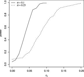
Figure 1: Power function of the test statistic $T_{1}$.

Example 4.3.

To study the finite-sample performance of the test statistic $T_{1}$ in Section 3.1, we consider the same model as that of scenario (i) in Example 4.2. Due to the model’s parameter setting, we naturally consider the following null and alternative hypotheses:

$$H_{0}\dvtx\beta_{3}=\beta_{4}=\beta_{5}=\beta_{7}=0\quad\mbox{versus}\quad H_{1}\dvtx\beta_{3}=\beta_{4}=\beta_{5}=\beta_{7}=c_{1},$$

where $c_{1}$ ranges from 0 to 0.1 with increment 0.01 for $\sigma=0.1$, whereas $c_{1}$ is the value from a set of $\{0,0.01,0.02,\ldots,0.09,0.15,0.2\}$ for $\sigma=0.25$. In addition, $500$ realizations were generated with $n=200$ to calculate the size and power of $T_{1}$. Figure 1 depicts the power function versus $c_{1}$. It shows that the empirical size at $c_{1}=0$ is very close to the nominal level 0.05. Furthermore, the power of the test is greater than $0.95$ as $c_{1}$ increases to $0.05$ and $0.15$, respectively, when $\sigma=0.1$ and $\sigma=0.25$. It is not surprising that the power increases as the signal gets stronger. In summary, $T_{1}$ not only controls the size well, but is also a powerful test.

Example 4.4.

To examine the performance of the test statistic $T_{2}$ in Section 3.2, we generated $500$ realizations from the model given below with $n=200$.

$$y=\eta\bigl{\{}(z_{1}+z_{2}+z_{3})/{\sqrt{3}}\bigr{\}}-0.5x_{1}+0.3x_{2}+\sigma\varepsilon,$$ (13)

where $\sigma=0.1$ and $\sigma=0.25$, respectively. We then consider the following hypotheses:

$$H_{0}\dvtx\eta(u)=u\quad\mbox{versus}\quad H_{1}\dvtx\eta(u)=c_{2}\sin\{\pi(u-a)/(b-a)\}+u,$$

where $c_{2}$ ranges from 0 to 0.1 with increment 0.025 for $\sigma=0.1$, while $c_{2}$ ranges from 0 to 0.2 with increment 0.05 for $\sigma=0.25$. Figure 2 demonstrates that the empirical size at $c_{2}=0$ is very close to the nominal level 0.05. Furthermore, the power of the test is greater than $0.95$ as $c_{2}$ increases to $0.075$ and $0.2$, respectively. As expected, the power increases when the signal becomes stronger. Although $T_{2}$ is slightly less powerful than $T_{1}$, it controls the size well and is a reliable test.

5 Discussion

In partially linear single-index models, we propose using the SCAD approach to shrink parameters contained in both parametric and nonpara- metric components. The resulting estimators enjoy the oracle property when the regularization parameters satisfy the proper conditions. To further exploit SCAD, one could extend the current results to partially linear multiple-index models by allowing $\varepsilon$ to be dependent on $(Z^{{\mathrm{T}}},X^{{\mathrm{T}}})^{{\mathrm{T}}}$. In addition, one could obtain the SCAD estimator for generalized partially linear single-index models. Finally, an investigation of partially linear single-index model selection with error-prone covariates could also be of interest. We believe that these efforts would enhance the usefulness of SCAD in data analysis.

Figure 2: Power function of the test statistic $T_{2}$.

Appendix: Proofs of theorems

.1 Proof of Theorem 1

Under the conditions of Theorem 1, we follow similar arguments to those used by Ichimura (1993) and show that $\hat{\bolds{\zeta}}=(\hat{\bolds{\alpha}}{}^{{\mathrm{T}}},\hat{{\bolds{\beta}}}{}^{\mathrm{T}})^{{\mathrm{T}}}$ is a root-$n$ consistent estimator of ${\bolds{\zeta}}$. Because the proof is straightforward, we do not present it here. We next demonstrate the asymptotic normality of $\hat{\bolds{\zeta}}$ by using a general result of Newey (1994).

Let $m_{x}(\Lambda)=E(X|\Lambda)$, $m_{z}(\Lambda)=E(Z|\Lambda)$ and $\kappa=\eta^{\prime}(\Lambda)\{Z-m_{z}(\Lambda)\}$. In addition, let

$$\Psi(m_{x},\eta,\kappa,{\bolds{\alpha}},{\bolds{\beta}},Y,Z,X)=(Y-\eta-X^{\mathrm{T}}{\bolds{\beta}})\left\{\matrix{\kappa\vspace*{4pt}\cr X-m_{x}(\Lambda)}\right\}.$$ (14)

For any given $m_{x}^{*}$, $\eta^{*}$ and $\kappa^{*}$, define

$$D(m_{x}^{*}-m_{x},\eta^{*}-\eta,\kappa^{*}-\kappa,{\bolds{\alpha}},{\bolds{\beta}},Y,Z,X)$$

$$\qquad=\frac{\partial\Psi}{\partial m_{x}}(m_{x}^{*}-m_{x})+\frac{\partial\Psi}{\partial\eta}(\eta^{*}-\eta)+\frac{\partial\Psi}{\partial\kappa}(\kappa^{*}-\kappa),$$

where the partial derivatives are the Frechet partial derivatives. After algebraic simplification, we have

$$\frac{\partial\Psi}{\partial m_{x}} = (Y-\eta-X^{\mathrm{T}}{\bolds{\beta}})\pmatrix{0\cr-1},$$

$$\frac{\partial\Psi}{\partial\eta} = -\left\{\matrix{\kappa\vspace*{2pt}\cr X-m_{x}(\Lambda)}\right\},$$

$$\frac{\partial\Psi}{\partial\kappa} = (Y-\eta-X^{\mathrm{T}}{\bolds{\beta}})\pmatrix{1\cr 0},$$

where the partial derivatives are zero. Accordingly,

$$\|\Psi(m^{*}_{x},\eta^{*},\kappa^{*},{\bolds{\alpha}},{\bolds{\beta}},Y,Z,X)-\Psi(m_{x},\eta,\kappa,{\bolds{\alpha}},{\bolds{\beta}},Y,Z,X)$$

$$\qquad\quad\hskip 24.0pt{}-D(m_{x}^{*}-m_{x},\eta^{*}-\eta,\kappa^{*}-\kappa,{\bolds{\alpha}},{\bolds{\beta}},Y,Z,X)\|$$ (15)

$$\qquad=O(\|m_{x}^{*}-m_{x}\|^{2}+\|\eta^{*}-\eta\|^{2}+\|\kappa^{*}-\kappa\|^{2}),$$

where $\|\cdot\|$ denotes the Sobolev norm, that is, the supremum norm of the function itself, as well as its derivatives. Equation (.1) is Newey’s Assumption 5.1(i). It is also noteworthy that his Assumption 5.2 holds by the expression of $D(\cdot,\cdot,\cdot,{\bolds{\alpha}},{\bolds{\beta}},Y,Z,X)$. Moreover, the result

$$E\{D(m_{x}^{*}-m_{x},\eta^{*}-\eta,\kappa^{*}-\kappa,{\bolds{\alpha}},{\bolds{\beta}},Y,Z,X)\}=0$$

leads to Newey’s Assumption 5.3.

In addition to Newey’s assumptions mentioned above, we need to verify one more assumption before employing his result. To this end, we re-express the solution of (2) as

$$\hat{\eta}(u)=\frac{1}{n}\sum_{i=1}^{n}\frac{\{\hat{s}_{2}(u,h)-\hat{s}_{1}(u,h)(\Lambda_{i}-u)\}K_{h}(\Lambda_{i}-u)(Y_{i}-X_{i}^{\mathrm{T}}{\bolds{\beta}})}{\hat{s}_{2}(u,h)\hat{s}_{0}(u,h)-\hat{s}_{1}^{2}(u,h)},$$

where $\Lambda_{i}$ is the $i$th row of $\Lambda$ and

$$\hat{s}_{r}(u,h)=\frac{1}{n}\sum_{i=1}^{n}(\Lambda_{i}-u)^{r}K_{h}(\Lambda_{i}-u)\qquad\mbox{for }r=0,1,2.$$

Then, let

$$\hat{m}_{x}(u) = \frac{1}{n}\sum_{i=1}^{n}\frac{\{\hat{s}_{2}(u,h)-\hat{s}_{1}(u,h)(\Lambda_{i}-u)\}K_{h}(\Lambda_{i}-u)X_{i}^{\mathrm{T}}}{\hat{s}_{2}(u,h)\hat{s}_{0}(u,h)-\hat{s}_{1}^{2}(u,h)},$$

$$\hat{m}_{z}(u) = \frac{1}{n}\sum_{i=1}^{n}\frac{\{\hat{s}_{2}(u,h)-\hat{s}_{1}(u,h)(\Lambda_{i}-u)\}K_{h}(\Lambda_{i}-u)Z_{i}^{\mathrm{T}}}{\hat{s}_{2}(u,h)\hat{s}_{0}(u,h)-\hat{s}_{1}^{2}(u,h)}.$$

Applying similar techniques to those used in Mack and Silverman (1982), we obtain the following equations, which hold uniformly in $u\in{\mathcal{U}}$:

$$\hat{\eta}(u)-\eta(u) = o_{p}(n^{-1/4}),\qquad\hat{\eta}^{\prime}(u)-\eta^{\prime}(u)=o_{p}(n^{-1/4}),$$

$$\hat{m}_{x}(u)-m_{x}(u) = o_{p}(n^{-1/4})\quad\mbox{and}\quad\hat{m}_{z}(u)-m_{z}(u)=o_{p}(n^{-1/4}).$$

These results imply that $\hat{\kappa}-\kappa=o_{p}(n^{-1/4})$. Thus, Newey’s Assumption 5.1(ii) holds.

After examining Newey’s Assumptions 5.1–5.3, we apply his Lemma 5.1 and find that $\hat{\bolds{\zeta}}$ has the same limit distribution as the solution to the equation

$$0=\sum_{i=1}^{n}\Psi(m_{x},\eta,\kappa,{\bolds{\alpha}},{\bolds{\beta}},Y_{i},Z_{i},X_{i}).$$ (17)

Furthermore, it is easy to show that the solution to (17) has the same limit distribution as described in the statement of Theorem 1. Hence, we complete the proof of asymptotic normality.

Finally, we show the efficiency of $\hat{\bolds{\zeta}}$. Let $p_{\varepsilon}(\varepsilon)$ be the probability density function of $\varepsilon$ and let $p^{\prime}_{\varepsilon}(\varepsilon)$ be its first-order derivative with respect to $\varepsilon$. Then, the score function of $({\bolds{\alpha}},{\bolds{\beta}})$ is

$$S_{({\bolds{\alpha}},{\bolds{\beta}})}=-\sigma^{2}\left\{\matrix{\eta^{\prime}(\Lambda)Z\vspace*{2pt}\cr X}\right\}\frac{p^{\prime}_{\varepsilon}(\varepsilon)}{p_{\varepsilon}(\varepsilon)}.$$

For any given function $g$ of $(Z,X)$, it can be shown that the nuisance tangent space ${\mathcal{P}}$, for the three nuisance parameters, $g_{(Z,X)}(z,x)$, $p_{\varepsilon}(\varepsilon)$ and $\eta(\Lambda)$, is $\{g(Z,X)\dvtx E(g)=0,E(\varepsilon g)$ is a function of $(Z,X)$ only$\}$. Furthermore, the orthogonal component of ${\mathcal{P}}$ is

$${\mathcal{P}}^{\bot}=\{\varepsilon g(Z,X)\dvtx E(g|\Lambda)=0\}.$$

Subsequently, we apply the approach of Bickel et al. (1993) and obtain the following semiparametric efficient score function via equation (4):

$$S_{\mathrm{eff}}=\varepsilon\left\{\matrix{\eta^{\prime}(\Lambda)\widetilde{Z}\vspace*{2pt}\cr\widetilde{X}}\right\}.$$ (18)

It can be seen that $S_{\mathrm{eff}}\in{\mathcal{P}}^{\bot}$.

For any $\varepsilon g\in{\mathcal{P}}^{\bot}$, we have $E(g|\Lambda)=0$. Accordingly,

$$E\bigl{\{}\bigl{(}S_{({\bolds{\alpha}},{\bolds{\beta}})}-S_{\mathrm{eff}}\bigr{)}^{\mathrm{T}}\varepsilon g(Z,X)\bigr{\}}$$

$$\qquad=E\left(-\sigma^{2}\left\{\matrix{\eta^{\prime}(\Lambda)Z\vspace*{2pt}\cr X}\right\}^{\mathrm{T}}gE\left\{\frac{\varepsilon p^{\prime}_{\varepsilon}(\varepsilon)}{p_{\varepsilon}(\varepsilon)}\right\}\right.$$

$$\qquad\quad\hskip 15.0pt{}-\left.E(\varepsilon^{2})\left[\left\{\matrix{\eta^{\prime}(\Lambda)Z\vspace*{2pt}\cr X}\right\}^{\mathrm{T}}g-E\left\{\matrix{\eta^{\prime}(\Lambda)E(Z|\Lambda)\vspace*{2pt}\cr E(X|\Lambda)}\right\}^{\mathrm{T}}g\right]\right).$$

Because $E\{{\varepsilon p^{\prime}_{\varepsilon}(\varepsilon)}/{p_{\varepsilon}(\varepsilon)}\}=-1$, it follows that

$$E\bigl{\{}\bigl{(}S_{({\bolds{\alpha}},{\bolds{\beta}})}-S_{\mathrm{eff}}\bigr{)}^{\mathrm{T}}\varepsilon g(Z,X)\bigr{\}}=E\bigl{[}\{\eta^{\prime}(\Lambda)E(Z^{\mathrm{T}}|\Lambda),E(X^{\mathrm{T}}|\Lambda)\}E(g|\Lambda)\bigr{]}=0.$$

That is, $S_{\mathrm{eff}}$ is the projection of $S_{({\bolds{\alpha}},{\bolds{\beta}})}$ onto ${\mathcal{P}}^{\bot}$ and the estimator $\hat{\bolds{\zeta}}$ is therefore efficient [see Bickel et al. (1993)]. We have thus completed the proof.

.2 Proof of Theorem 2

To prove this theorem, we consider the following three steps: Step I establishes the order of the minimizer $(\hat{\bolds{\alpha}}{}^{{\mathrm{T}}}_{\lambda_{1}},\hat{{\bolds{\beta}}}{}^{{\mathrm{T}}}_{\lambda_{2}})^{{\mathrm{T}}}$ of ${\mathcal{L}}_{P}({\bolds{\alpha}},{\bolds{\beta}})$; Step II shows that $(\hat{\bolds{\alpha}}{}^{{\mathrm{T}}}_{\lambda_{1}},\hat{{\bolds{\beta}}}{}^{{\mathrm{T}}}_{\lambda_{2}})^{{\mathrm{T}}}$ attains sparsity; Step III derives the asymptotic distribution of the penalized estimators.

Step I. Let $\gamma_{n}=n^{-1/2}+a_{n}+c_{n}$, $\mathbf{v}_{1}=(v_{11},\ldots,v_{1p})^{{\mathrm{T}}}$, $\mathbf{v}_{2}=(v_{21},\ldots,v_{2q})^{{\mathrm{T}}}$ and $\|\mathbf{v}_{1}\|=\|\mathbf{v}_{2}\|=C$ for some positive constant $C$, where

$$a_{n} = \max_{1\leq j\leq p}\{|p_{\lambda_{1j}}^{\prime}(|\alpha_{0j}|)|,\alpha_{0j}\neq 0\},$$

$$c_{n} = \max_{1\leq k\leq q}\{|p_{\lambda_{2k}}^{\prime}(|\beta_{0k}|)|,\beta_{0k}\neq 0\},$$

and $\alpha_{0j}$ and $\beta_{0k}$ are the $j$th and $k$th elements of ${\bolds{\alpha}}_{0}$ and ${\bolds{\beta}}_{0}$, respectively, for $j=1,\ldots,p$ and $k=1,\ldots,q$. Furthermore, define

$$D_{n,1} = \sum_{i=1}^{n}\bigl{\{}Y_{i}-\hat{\eta}\bigl{(}Z_{i}^{\mathrm{T}}({\bolds{\alpha}}_{0}+\gamma_{n}\mathbf{v}_{1}),{\bolds{\alpha}}_{0}+\gamma_{n}\mathbf{v}_{1},{\bolds{\beta}}_{0}+\gamma_{n}\mathbf{v}_{2}\bigr{)}-X_{i}^{\mathrm{T}}({\bolds{\beta}}_{0}+\gamma_{n}\mathbf{v}_{2})\bigr{\}}^{2}$$

$${}-\sum_{i=1}^{n}\{Y_{i}-\hat{\eta}(X_{i}^{\mathrm{T}}{\bolds{\alpha}}_{0},{\bolds{\alpha}}_{0},{\bolds{\beta}}_{0})-X_{i}^{\mathrm{T}}{\bolds{\beta}}_{0}\}^{2}$$

and

$$D_{n,2} = -n\sum_{j=1}^{p_{0}}\{p_{\lambda_{1j}}(|\alpha_{0j}+\gamma_{n}v_{1j}|)-p_{\lambda_{1j}}(|\alpha_{0j}|)\}$$

$${}-n\sum_{k=1}^{q_{0}}\{p_{\lambda_{2k}}(|\beta_{0k}+\gamma_{n}v_{2k}|)-p_{\lambda_{2k}}(|\beta_{0k}|)\}.$$

After algebraic simplification, we have

$$D_{n,1} = \sum_{i=1}^{n}\bigl{\{}\hat{\eta}\bigl{(}Z_{i}^{\mathrm{T}}({\bolds{\alpha}}_{0}+\gamma_{n}\mathbf{v}_{1}),{\bolds{\alpha}}_{0}+\gamma_{n}\mathbf{v}_{1},{\bolds{\beta}}_{0}+\gamma_{n}\mathbf{v}_{2}\bigr{)}$$

$$\hphantom{\sum_{i=1}^{n}}\hskip 51.0pt{}-\hat{\eta}(Z_{i}^{\mathrm{T}}{\bolds{\alpha}}_{0},{\bolds{\alpha}}_{0},{\bolds{\beta}}_{0})+X_{i}^{\mathrm{T}}\gamma_{n}\mathbf{v}_{2}\bigr{\}}$$

$$\hphantom{\sum_{i=1}^{n}}{}\times\bigl{\{}\hat{\eta}\bigl{(}Z_{i}^{\mathrm{T}}({\bolds{\alpha}}_{0}+\gamma_{n}\mathbf{v}_{1}),{\bolds{\alpha}}_{0}+\gamma_{n}\mathbf{v}_{1},{\bolds{\beta}}_{0}+\gamma_{n}\mathbf{v}_{2}\bigr{)}$$

$$\hphantom{\sum_{i=1}^{n}}\hskip 14.0pt{}+\hat{\eta}(Z_{i}^{\mathrm{T}}{\bolds{\alpha}}_{0},{\bolds{\alpha}}_{0},{\bolds{\beta}}_{0})+X_{i}^{\mathrm{T}}({\bolds{\beta}}_{0}+\gamma_{n}\mathbf{v}_{2})+X_{i}^{\mathrm{T}}{\bolds{\beta}}_{0}-2Y_{i}\bigr{\}}$$

$$= \sum_{i=1}^{n}\{\widetilde{Z}_{i}^{\mathrm{T}}\eta^{\prime}(\Lambda_{i})\mathbf{v}_{1}\gamma_{n}+\widetilde{X}_{i}^{\mathrm{T}}\mathbf{v}_{2}\gamma_{n}\}^{2}$$

$${}-\sum_{i=1}^{n}\{\widetilde{Z}_{i}^{\mathrm{T}}\eta^{\prime}(\Lambda_{i})\mathbf{v}_{1}\gamma_{n}+\widetilde{X}_{i}^{\mathrm{T}}\mathbf{v}_{2}\gamma_{n}\}\varepsilon_{i}+o_{p}(1).$$

Moreover, applying the Taylor expansion and the Cauchy–Schwarz inequality, we are able to show that $n^{-1}D_{n,2}$ is bounded by

$$\sqrt{p_{0}}\gamma_{n}a_{n}\|\mathbf{v}_{1}\|+\gamma_{n}^{2}b_{n}\|\mathbf{v}_{1}\|^{2}+\sqrt{q_{0}}\gamma_{n}c_{n}\|\mathbf{v}_{2}\|+\gamma_{n}^{2}d_{n}\|\mathbf{v}_{2}\|^{2}$$

$$\qquad\leq C\gamma_{n}^{2}\bigl{(}\sqrt{p_{0}}+b_{n}C+\sqrt{q_{0}}+d_{n}C\bigr{)},$$

where

$$b_{n}=\max_{1\leq j\leq p}\{|p_{\lambda_{1j}}^{\prime\prime}(|\alpha_{0j}|)|,\alpha_{0j}\neq 0\},\qquad d_{n}=\max_{1\leq k\leq q}\{|p_{\lambda_{2k}}^{\prime\prime}(|\beta_{0k}|)|,\beta_{0k}\neq 0\}.$$

When $b_{n}$ and $d_{n}$ tend to $0$ and $C$ is sufficiently large, the first term on the right-hand side of (.2) dominates the second term on the right-hand side of (.2) and $D_{n,2}$. As a result, for any given $\nu>0$, there exists a large constant $C$ such that

$$P\Bigl{\{}\inf_{{\mathcal{V}}_{12}}{\mathcal{L}}_{P}({\bolds{\alpha}}_{0}+\gamma_{n}\mathbf{v}_{1},{\bolds{\beta}}_{0}+\gamma_{n}\mathbf{v}_{2})>{\mathcal{L}}_{P}({\bolds{\alpha}}_{0},{\bolds{\beta}}_{0})\Bigr{\}}\geq 1-\nu,$$

where ${\mathcal{V}}_{12}=\{(\mathbf{v}_{1},\mathbf{v}_{2})\dvtx\|\mathbf{v}_{1}\|=C,\|\mathbf{v}_{2}\|=C\}$. We therefore conclude that the rate of convergence of $(\hat{{\bolds{\alpha}}}{}^{\mathrm{T}}_{\lambda_{1}},\hat{{\bolds{\beta}}}{}^{{\mathrm{T}}}_{\lambda_{2}})^{{\mathrm{T}}}$ is $O_{P}(n^{-1/2}+a_{n}+c_{n})$.

Step II. Let ${\bolds{\alpha}}_{1}$ and ${\bolds{\beta}}_{1}$ satisfy $\|{\bolds{\alpha}}_{1}-{\bolds{\alpha}}_{10}\|=O_{P}(n^{-1/2})$ and $\|{\bolds{\beta}}_{1}-{\bolds{\beta}}_{10}\|=O_{P}(n^{-1/2})$, respectively. We next show that

$${\mathcal{L}}_{P}\left\{\pmatrix{{\bolds{\alpha}}_{1}\cr{\mathbf{0}}},\pmatrix{{\bolds{\beta}}_{1}\cr{\mathbf{0}}}\right\}=\min_{\mathcal{C}}{\mathcal{L}}_{P}\left\{\pmatrix{{\bolds{\alpha}}_{1}\cr{\bolds{\alpha}}_{2}},\pmatrix{{\bolds{\beta}}_{1}\cr{\bolds{\beta}}_{2}}\right\},$$ (20)

where ${\mathcal{C}}=\{\|{\bolds{\alpha}}_{2}\|\leq C^{*}n^{-1/2},\|{\bolds{\beta}}_{2}\|\leq C^{*}n^{-1/2}\}$ and $C^{*}$ is a positive constant.

Consider $\beta_{k}\in(-C^{*}n^{-1/2},C^{*}n^{-1/2})$ for $k=q_{0}+1,\ldots,q$. When $\beta_{k}\neq 0$, we have ${\partial{\mathcal{L}}_{P}({\bolds{\alpha}},{\bolds{\beta}})}/{\partial\beta_{k}}=\ell_{k}({\bolds{\alpha}},{\bolds{\beta}})+np_{\lambda_{2k}}^{\prime}(|\beta_{k}|)\operatorname{sgn}(\beta_{k})$, where

$$\ell_{k}({\bolds{\alpha}},{\bolds{\beta}}) = \frac{1}{n}\sum_{i=1}^{n}\{Y_{i}-\hat{\eta}(Z_{i}^{\mathrm{T}}{\bolds{\alpha}},{\bolds{\alpha}},{\bolds{\beta}})+X_{i}^{\mathrm{T}}{\bolds{\beta}}\}\biggl{\{}X_{ik}+\frac{\partial\hat{\eta}(Z_{i}^{\mathrm{T}}{\bolds{\alpha}},{\bolds{\alpha}},{\bolds{\beta}})}{\partial\beta_{k}}\biggr{\}}$$

$$= \frac{1}{n}\sum_{i=1}^{n}\{\hat{\eta}(Z_{i}^{\mathrm{T}}{\bolds{\alpha}},{\bolds{\alpha}},{\bolds{\beta}})-\eta(Z_{i}^{\mathrm{T}}{\bolds{\alpha}}_{0})+X_{i}^{\mathrm{T}}({\bolds{\beta}}-{\bolds{\beta}}_{0})-\varepsilon_{i}\}$$

$$\phantom{\frac{1}{n}\sum_{i=1}^{n}}{}\times\biggl{\{}X_{ik}+\frac{\partial\hat{\eta}(Z_{i}^{\mathrm{T}}{\bolds{\alpha}},{\bolds{\alpha}},{\bolds{\beta}})}{\partial\beta_{k}}\biggr{\}}.$$

Applying arguments similar to those used in the proof of Theorem 5.2 of Ichimura (1993), together with algebraic simplifications, the above term can be expressed as

$$\frac{1}{n}\sum_{i=1}^{n}({\bolds{\alpha}}-{\bolds{\alpha}}_{0})^{\mathrm{T}}\widetilde{Z}_{i}\eta^{\prime}(\Lambda_{i})\widetilde{X}_{ik}+\frac{1}{n}\sum_{i=1}^{n}({\bolds{\beta}}-{\bolds{\beta}}_{0})^{\mathrm{T}}\widetilde{X}_{i}\widetilde{X}_{ik}+o_{p}(n^{-1/2}).$$

Using the assumptions that $\|{\bolds{\alpha}}-{\bolds{\alpha}}_{0}\|=O_{P}(n^{-1/2})$ and $\|{\bolds{\beta}}-{\bolds{\beta}}_{0}\|=O_{P}(n^{-1/2})$, we have that $n^{-1}\ell_{k}({\bolds{\alpha}},{\bolds{\beta}})$ is of the order $O_{P}(n^{-1/2})$. Therefore,

$$\frac{\partial\mathcal{L}_{P}({\bolds{\alpha}},{\bolds{\beta}})}{\partial\beta_{k}}=-n\lambda_{2k}\{\lambda_{2k}^{-1}p_{\lambda_{2k}}^{\prime}(|\beta_{k}|)\operatorname{sgn}(\beta_{k})+O_{P}(n^{-1/2}\lambda_{2k}^{-1})\}.$$

Because $\liminf_{n\to\infty}\liminf_{\beta_{j}\to 0^{+}}\lambda_{2k}^{-1}p_{\lambda_{2k}}^{\prime}(|\beta_{k}|)>0$ and $n^{-1/2}/{\lambda_{2k}}\to 0$,${\partial{\mathcal{L}}_{P}({\bolds{\alpha}},{\bolds{\beta}})}/{\partial\beta_{k}}$ and $\beta_{k}$ have different signs for $\beta_{k}\in(-C^{*}n^{-1/2},C^{*}n^{-1/2})$. Analogously, we can show that ${\partial{\mathcal{L}}_{P}({\bolds{\alpha}},{\bolds{\beta}})}/{\partial\alpha_{j}}$ and $\alpha_{j}$ have different signs when $\alpha_{j}\in(-C^{*}n^{-1/2},C^{*}n^{-1/2})$ for $j=p_{0}+1,\ldots,p$. Consequently, the minimum is attained at ${\bolds{\alpha}}_{2}=0$ and ${\bolds{\beta}}_{2}=0$. This completes the proof of (20).

Step III. Finally, we demonstrate the asymptotic normality of $\hat{\bolds{\alpha}}_{{\lambda_{1}}1}$ and $\hat{\bolds{\beta}}_{{\lambda_{2}}1}$. For the sake of simplicity, we define

$${\mathbf{R}_{\lambda_{1}}} = \{p_{\lambda_{11}}^{\prime}(|\alpha_{01}|)\operatorname{sgn}(\alpha_{01}),\ldots,p_{\lambda_{1{p_{0}}}}^{\prime}(|\alpha_{0{p_{0}}}|)\operatorname{sgn}(\alpha_{0{p_{0}}})\}^{\mathrm{T}},$$

$$\Sigma_{\lambda_{1}} = \operatorname{diag}\{p_{\lambda_{11}}^{\prime\prime}(|\alpha_{01}|),\ldots,p_{\lambda_{1{p_{0}}}}^{\prime\prime}(|\alpha_{0{p_{0}}}|)\},$$

$${\mathbf{R}_{\lambda_{2}}} = \{p_{\lambda_{21}}^{\prime}(|\beta_{01}|)\operatorname{sgn}(\beta_{01}),\ldots,p_{\lambda_{2{q_{0}}}}^{\prime}(|\beta_{0{q_{0}}}|)\operatorname{sgn}(\beta_{0{q_{0}}})\}^{\mathrm{T}},$$

$$\Sigma_{\lambda_{2}} = \operatorname{diag}\{p_{\lambda_{21}}^{\prime\prime}(|\beta_{01}|),\ldots,p_{\lambda_{2{q_{0}}}}^{\prime\prime}(|\beta_{0{q_{0}}}|)\},$$

where $\alpha_{0j}$ and $\beta_{0k}$ are the $j$th and $k$th elements of ${\bolds{\alpha}}_{10}$ and ${\bolds{\beta}}_{10}$, respectively, for $j=1,\ldots,p_{0}$ and $k=1,\ldots,q_{0}$. It follows from (5) that $\hat{\bolds{\alpha}}_{{\lambda_{1}}1}$ and $\hat{\bolds{\beta}}_{{\lambda_{2}}1}$ satisfy

$${\mathbf{0}} = \left\{\matrix{\dfrac{\partial{\mathcal{L}}_{P}(\hat{\bolds{\alpha}}_{{\lambda_{1}}1},\hat{\bolds{\beta}}_{{\lambda_{2}}1})}{\partial{\bolds{\alpha}}_{1}}\vspace*{2pt}\cr\dfrac{\partial{\mathcal{L}}_{P}(\hat{\bolds{\alpha}}_{{\lambda_{1}}1},\hat{\bolds{\beta}}_{{\lambda_{2}}1})}{\partial{\bolds{\beta}}_{1}}}\right\}$$

$$= l(\hat{\bolds{\alpha}}_{{\lambda_{1}}1},\hat{\bolds{\beta}}_{{\lambda_{2}}1})+\left\{\matrix{\mathbf{R}_{\lambda_{1}}-\Sigma_{\lambda_{1}}(\hat{\bolds{\alpha}}_{{\lambda_{1}}1}-{\bolds{\alpha}}_{10})\vspace*{2pt}\cr\mathbf{R}_{\lambda_{2}}-\Sigma_{\lambda_{2}}(\hat{\bolds{\beta}}_{{\lambda_{2}}1}-{\bolds{\beta}}_{10})}\right\},$$

where

$$l(\hat{\bolds{\alpha}}_{{\lambda_{1}}1},\hat{\bolds{\beta}}_{{\lambda_{2}}1})=\frac{1}{n}\sum_{i=1}^{n}\{Y_{i}-\hat{\eta}(\Lambda_{i},\hat{\bolds{\zeta}}_{\lambda 1})-X_{i,1}^{\mathrm{T}}\hat{\bolds{\beta}}_{{\lambda_{2}}1}\}\left\{\matrix{\dfrac{\partial\hat{\eta}(\hat{\Lambda}_{i},\hat{\bolds{\zeta}}_{\lambda 1})}{\partial{\bolds{\alpha}}}\vspace*{2pt}\cr\dfrac{\partial\hat{\eta}(\hat{\Lambda}_{i},\hat{\bolds{\zeta}}_{\lambda 1})}{\partial{\bolds{\beta}}}+X_{i,1}}\right\},$$

$\hat{\Lambda}_{i}$ and $X_{i,1}$ here being the $i$th rows of $\hat{\Lambda}$ and $X_{1}$, respectively, and $\hat{\bolds{\zeta}}_{\lambda 1}=(\hat{\bolds{\alpha}}{}^{{\mathrm{T}}}_{{\lambda_{1}}1},\hat{{\bolds{\beta}}}{}^{{\mathrm{T}}}_{{\lambda_{2}}1})^{{\mathrm{T}}}$ being the penalized least-squares estimator of ${\bolds{\zeta}}_{1}=({\bolds{\alpha}}_{1}^{{\mathrm{T}}},{\bolds{\beta}}_{1}^{{\mathrm{T}}})^{{\mathrm{T}}}$.

Applying the Taylor expansion, we obtain

$$l(\hat{\bolds{\alpha}}_{{\lambda_{1}}1},\hat{\bolds{\beta}}_{{\lambda_{2}}1}) = \frac{1}{n}\sum_{i=1}^{n}\{Y_{i}-\hat{\eta}(\Lambda_{i},{\bolds{\zeta}}_{1})-X_{i,1}^{\mathrm{T}}{\bolds{\beta}}_{1}\}\left\{\matrix{\dfrac{\partial\hat{\eta}(\Lambda_{i},{\bolds{\zeta}}_{1})}{\partial{\bolds{\alpha}}_{1}}\vspace*{2pt}\cr\dfrac{\partial\hat{\eta}(\Lambda_{i},{\bolds{\zeta}}_{1})}{\partial{\bolds{\beta}}_{1}}+X_{i,1}}\right\}$$

$${}-\frac{1}{n}\sum_{i=1}^{n}\left\{\matrix{\dfrac{\partial\hat{\eta}(\bar{\Lambda}_{i},\bar{\bolds{\zeta}}_{1})}{\partial{\bolds{\alpha}}_{1}}\vspace*{2pt}\cr\dfrac{\partial\hat{\eta}(\bar{\Lambda}_{i},\bar{\bolds{\zeta}}_{1})}{\partial{\bolds{\beta}}_{1}}+X_{i,1}}\right\}^{\otimes 2}(\hat{\bolds{\zeta}}_{\lambda 1}-{\bolds{\zeta}}_{1})$$

$${}-\frac{1}{n}\sum_{i=1}^{n}\{Y_{i}-\hat{\eta}(\bar{\Lambda}_{i},\bar{\bolds{\zeta}}_{1})-X_{i,1}^{\mathrm{T}}\bar{\bolds{\beta}}_{1}\}\frac{\partial^{2}\hat{\eta}(\bar{\Lambda}_{i},\bar{\bolds{\zeta}}_{1})}{\partial{\bolds{\zeta}}_{1}\,\partial{\bolds{\zeta}}_{1}^{\mathrm{T}}}(\hat{\bolds{\zeta}}_{\lambda 1}-{\bolds{\zeta}}_{1}),$$

where $\bar{\bolds{\beta}}_{1}$, $\bar{\Lambda}_{i}$ and $\bar{\bolds{\zeta}}_{1}$ are the interior points between ${\bolds{\beta}}_{1}$ and $\hat{\bolds{\beta}}_{{\lambda_{2}}1}$, $\Lambda_{i}$ and $\hat{\Lambda}_{i}$, and ${\bolds{\zeta}}_{1}$ and $\hat{\bolds{\zeta}}_{\lambda 1}$, respectively. Furthermore, using arguments similar to those used in the proof of Theorem 1, we have that

$$l(\hat{\bolds{\alpha}}_{{\lambda_{1}}1},\hat{\bolds{\beta}}_{{\lambda_{2}}1}) = \frac{1}{\sqrt{n}}\sum_{i=1}^{n}\left\{\matrix{\widetilde{Z}_{i,1}\eta^{\prime}(\Lambda_{i})\vspace*{2pt}\cr\widetilde{X}_{i,1}}\right\}\varepsilon_{i}$$

$${}-\frac{1}{n}\sum_{i=1}^{n}\left\{\matrix{\widetilde{Z}_{i,1}\eta^{\prime}(\Lambda_{i})\vspace*{2pt}\cr\widetilde{X}_{i,1}}\right\}^{\otimes 2}\sqrt{n}\pmatrix{\hat{\bolds{\alpha}}_{{\lambda_{1}}1}-{\bolds{\alpha}}_{10}\vspace*{2pt}\cr\hat{\bolds{\beta}}_{{\lambda_{2}}1}-{\bolds{\beta}}_{10}}+o_{p}(1).$$

Moreover, the summand of the matrix over $n$ in the second term of the above equation converges to $\left({{\Gamma_{\widetilde{Z}_{1}\widetilde{Z}_{1}}\enskip\Gamma_{\widetilde{X}_{1}\widetilde{Z}_{1}}}\atop{\Gamma_{\widetilde{X}_{1}\widetilde{Z}_{1}}^{{\mathrm{T}}}\enskip\Gamma_{\widetilde{X}_{1}\widetilde{X}_{1}}}}\right)$. These results, together with (.2), lead to

$$n^{1/2}\pmatrix{\Gamma_{\widetilde{Z}_{1}\widetilde{Z}_{1}}+\Sigma_{\lambda_{1}}&\Gamma_{\widetilde{X}_{1}\widetilde{Z}_{1}}\vspace*{2pt}\cr\Gamma_{\widetilde{X}_{1}\widetilde{Z}_{1}}^{{\mathrm{T}}}&\Gamma_{\widetilde{X}_{1}\widetilde{X}_{1}}+\Sigma_{\lambda_{2}}}\pmatrix{\hat{\bolds{\alpha}}_{{\lambda_{1}}1}-{\bolds{\alpha}}_{10}\vspace*{2pt}\cr\hat{\bolds{\beta}}_{{\lambda_{2}}1}-{\bolds{\beta}}_{10}}-n^{1/2}\pmatrix{{\mathbf{R}_{\lambda_{1}}}\vspace*{2pt}\cr{\mathbf{R}_{\lambda_{2}}}}$$

$$\qquad=\frac{1}{\sqrt{n}}\sum_{i=1}^{n}\left\{\matrix{\widetilde{Z}_{i,1}\eta^{\prime}(\Lambda_{i})\varepsilon_{i}\vspace*{2pt}\cr\widetilde{X}_{i,1}\varepsilon_{i}}\right\}+o_{p}(1).$$

It follows that

$$n^{1/2}(\Gamma_{\widetilde{Z}_{1}\widetilde{Z}_{1}}+\Sigma_{\lambda_{1}})(\hat{\bolds{\alpha}}_{{\lambda_{1}}1}-{\bolds{\alpha}}_{10})+n^{1/2}\Gamma_{\widetilde{X}_{1}\widetilde{Z}_{1}}(\hat{\bolds{\beta}}_{{\lambda_{2}}1}-{\bolds{\beta}}_{10})-n^{1/2}{\mathbf{R}_{\lambda_{1}}}$$

$$\qquad=\frac{1}{\sqrt{n}}\sum_{i=1}^{n}\widetilde{Z}_{i,1}\eta^{\prime}(\Lambda_{i})\varepsilon_{i}+o_{p}(1)$$

and

$$n^{1/2}\Gamma_{\widetilde{X}_{1}\widetilde{Z}_{1}}^{{\mathrm{T}}}(\hat{\bolds{\alpha}}_{{\lambda_{1}}1}-{\bolds{\alpha}}_{10})+n^{1/2}(\Gamma_{\widetilde{X}_{1}\widetilde{X}_{1}}+\Sigma_{\lambda_{2}})(\hat{\bolds{\beta}}_{{\lambda_{2}}1}-{\bolds{\beta}}_{10})-n^{1/2}{\mathbf{R}_{\lambda_{2}}}$$

$$\qquad=\frac{1}{\sqrt{n}}\sum_{i=1}^{n}\widetilde{X}_{i,1}\varepsilon_{i}+o_{p}(1).$$

After simplification, we have

$$\sqrt{n}\{(\Gamma_{\widetilde{Z}_{1}\widetilde{Z}_{1}}+\Sigma_{\lambda_{1}})-\Gamma_{\widetilde{X}_{1}\widetilde{Z}_{1}}(\Gamma_{\widetilde{X}_{1}\widetilde{X}_{1}}+\Sigma_{\lambda_{2}})^{-1}\Gamma_{\widetilde{X}_{1}\widetilde{Z}_{1}}^{\mathrm{T}}\}(\hat{\bolds{\alpha}}_{{\lambda_{1}}1}-{\bolds{\alpha}}_{10})$$

$$\quad{}+n^{1/2}\{\Gamma_{\widetilde{X}_{1}\widetilde{Z}_{1}}(\Gamma_{\widetilde{X}_{1}\widetilde{X}_{1}}+\Sigma_{\lambda_{1}})^{-1}{\mathbf{R}_{\lambda_{1}}}-{\mathbf{R}_{\lambda_{2}}}\}$$

$$\qquad=\frac{1}{\sqrt{n}}\sum_{i=1}^{n}\{\widetilde{Z}_{i,1}\eta^{\prime}(\Lambda_{i})-\Gamma_{\widetilde{X}_{1}\widetilde{Z}_{1}}(\Gamma_{\widetilde{X}_{1}\widetilde{X}_{1}}+\Sigma_{\lambda_{2}})^{-1}\widetilde{X}_{i,1}\}\varepsilon_{i}+o_{p}(1)$$

and

$$\sqrt{n}\{(\Gamma_{\widetilde{X}_{1}\widetilde{X}_{1}}+\Sigma_{\lambda_{2}})-\Gamma_{\widetilde{X}_{1}\widetilde{Z}_{1}}^{\mathrm{T}}(\Gamma_{\widetilde{Z}_{1}\widetilde{Z}_{1}}+\Sigma_{\lambda_{1}})^{-1}\Gamma_{\widetilde{X}_{1}\widetilde{Z}_{1}}\}(\hat{\bolds{\beta}}_{{\lambda_{2}}1}-{\bolds{\beta}}_{10})$$

$$\quad{}+n^{1/2}\{\Gamma_{\widetilde{X}_{1}\widetilde{Z}_{1}}^{\mathrm{T}}(\Gamma_{\widetilde{Z}_{1}\widetilde{Z}_{1}}+\Sigma_{\lambda_{1}})^{-1}{\mathbf{R}_{\lambda_{2}}}-{\mathbf{R}_{\lambda_{1}}}\}$$

$$\qquad=\frac{1}{\sqrt{n}}\sum_{i=1}^{n}\{\widetilde{X}_{i,1}-\Gamma_{\widetilde{X}_{1}\widetilde{Z}_{1}}^{{\mathrm{T}}}(\Gamma_{\widetilde{Z}_{1}\widetilde{Z}_{1}}+\Sigma_{\lambda_{1}})^{-1}\widetilde{Z}_{i,1}\eta^{\prime}(\Lambda_{i})\}\varepsilon_{i}+o_{p}(1).$$

Equations (.2) and (.2), together with the central limit theorem, yield that

$$\sqrt{n}\{\Gamma_{\widetilde{Z}_{1}\widetilde{Z}_{1}}+\Sigma_{\lambda_{1}}-\Gamma_{\widetilde{X}_{1}\widetilde{Z}_{1}}(\Gamma_{\widetilde{X}_{1}\widetilde{X}_{1}}+\Sigma_{\lambda_{2}})^{-1}\Gamma_{\widetilde{X}_{1}\widetilde{Z}_{1}}^{\mathrm{T}}\}(\hat{\bolds{\alpha}}_{{\lambda_{1}}1}-{\bolds{\alpha}}_{10})$$

$$\qquad{}+n^{1/2}\{\Gamma_{\widetilde{X}_{1}\widetilde{Z}_{1}}(\Gamma_{\widetilde{X}_{1}\widetilde{X}_{1}}+\Sigma_{\lambda_{2}})^{-1}\mathbf{R}_{\lambda_{1}}-\mathbf{R}_{\lambda_{2}}\}\to N(0,\Sigma_{\mathop{{\bolds{\alpha}}}_{1}})$$

and

$$\sqrt{n}\{\Gamma_{\widetilde{X}_{1}\widetilde{X}_{1}}+\Sigma_{\lambda_{2}}-\Gamma_{\widetilde{X}_{1}\widetilde{Z}_{1}}^{\mathrm{T}}(\Gamma_{\widetilde{Z}_{1}\widetilde{Z}_{1}}+\Sigma_{\lambda_{1}})^{-1}\Gamma_{\widetilde{X}_{1}\widetilde{Z}_{1}}\}(\hat{\bolds{\beta}}_{{\lambda_{2}}1}-{\bolds{\beta}}_{10})$$

$$\qquad{}+n^{1/2}\{\Gamma_{\widetilde{X}_{1}\widetilde{Z}_{1}}^{\mathrm{T}}(\Gamma_{\widetilde{Z}_{1}\widetilde{Z}_{1}}+\Sigma_{\lambda_{1}})^{-1}\mathbf{R}_{\lambda_{2}}-\mathbf{R}_{\lambda_{1}}\}\to N(0,\Sigma_{\mathop{{\bolds{\beta}}}_{1}}),$$

where

$$\Sigma_{\mathop{{\bolds{\alpha}}}_{1}} = \{\Gamma_{\widetilde{Z}_{1}\widetilde{Z}_{1}}-2\Gamma_{\widetilde{X}_{1}\widetilde{Z}_{1}}(\Gamma_{\widetilde{X}_{1}\widetilde{X}_{1}}+\Sigma_{\lambda_{2}})^{-1}\Gamma_{\widetilde{X}_{1}\widetilde{Z}_{1}}^{\mathrm{T}}$$

$${}+\Gamma_{\widetilde{X}_{1}\widetilde{Z}_{1}}(\Gamma_{\widetilde{X}_{1}\widetilde{X}_{1}}+\Sigma_{\lambda_{2}})^{-1}\Gamma_{\widetilde{X}_{1}\widetilde{X}_{1}}(\Gamma_{\widetilde{X}_{1}\widetilde{X}_{1}}+\Sigma_{\lambda_{2}})^{-1}\Gamma_{\widetilde{X}_{1}\widetilde{Z}_{1}}^{\mathrm{T}}\}\sigma^{2}$$

and

$$\Sigma_{\mathop{{\bolds{\beta}}}_{1}} = \{\Gamma_{\widetilde{X}_{1}\widetilde{X}_{1}}-2\Gamma_{\widetilde{X}_{1}\widetilde{Z}_{1}}^{\mathrm{T}}(\Gamma_{\widetilde{Z}_{1}\widetilde{Z}_{1}}+\Sigma_{\lambda_{1}})^{-1}\Gamma_{\widetilde{X}_{1}\widetilde{Z}_{1}}$$

$${}+\Gamma_{\widetilde{X}_{1}\widetilde{Z}_{1}}^{\mathrm{T}}(\Gamma_{\widetilde{Z}_{1}\widetilde{Z}_{1}}+\Sigma_{\lambda_{1}})^{-1}\Gamma_{\widetilde{Z}_{1}\widetilde{Z}_{1}}(\Gamma_{\widetilde{Z}_{1}\widetilde{Z}_{1}}+\Sigma_{\lambda_{1}})^{-1}\Gamma_{\widetilde{X}_{1}\widetilde{Z}_{1}}\}\sigma^{2}.$$

Because each element of $n^{1/2}\Sigma_{\lambda_{1}}$, $n^{1/2}\Sigma_{\lambda_{2}}$, $n^{1/2}\mathbf{R}_{\lambda_{1}}$ and $n^{1/2}\mathbf{R}_{\lambda_{2}}$ tends to zero, we complete the proof.

.3 Proof of Theorem 3

Let $\tau_{n}=\log(n)$, $\lambda_{n1j}=\tau_{n}\operatorname{SE}(\hat{\alpha}_{j}^{u})$, $\lambda_{n2k}=\tau_{n}\operatorname{SE}(\hat{\beta}_{k}^{u})$ and

$$\operatorname{BIC}(S_{T})=\log\{\sigma_{n}^{2}(S_{T})\}+\{\log(n)/n\}\operatorname{DF}(S_{T}),$$

where $\operatorname{DF}(S_{T})$ stands for the degrees of freedom of the true model $S_{T}$. $\operatorname{SE}(\hat{\alpha}_{k}^{u})=O(1/\sqrt{n})$ and $\operatorname{SE}(\hat{\beta}_{j}^{u})=O(1/\sqrt{n})$. Thus, $\lambda_{n1j}=O_{P}(\log(n)/\sqrt{n})$ and $\lambda_{n2k}=O_{P}(\log(n)/\sqrt{n})$. Then, employing techniques similar to those used in Wang, Li and Tsai (2007), we obtain that

$$P\{\operatorname{BIC}(\tau_{n})=\operatorname{BIC}(S_{T})\}=1.$$ (24)

Therefore, to prove the theorem, it suffices to show that

$$P\Bigl{\{}\inf_{\lambda\in\Omega_{-}\cup\Omega_{+}}\operatorname{BIC}(\lambda)>\operatorname{BIC}(\tau_{n})\Bigr{\}}\to 1,$$ (25)

where

$$\Omega_{-}=\{\lambda\dvtx S_{\lambda}\not\supset S_{T}\}\quad\mbox{and}\quad\Omega_{+}=\{\lambda\dvtx S_{\lambda}\supset S_{T}\}$$

represent the underfitted and overfitted models, respectively.

To demonstrate (25), we consider two separate cases given below.

Case 1: Underfitted model (i.e., the model misses at least one covariate from the true model). For any $\lambda\in\Omega_{-}$, (24). together with assumptions (A) and (B), implies that, with probability tending to one,

$$\operatorname{BIC}(\lambda)-\operatorname{BIC}(\tau_{n}) = \log\{\operatorname{MSE}(\lambda)\}+\{\log(n)/n\}\operatorname{DF}_{\lambda}-\operatorname{BIC}(S_{T})$$

$$\geq \log\{\operatorname{MSE}(\lambda)\}-\operatorname{BIC}(S_{T})$$

$$\geq \log\{\sigma_{n}^{2}(S_{\lambda})\}-\operatorname{BIC}(S_{T})$$

$$\geq \inf_{\lambda\in\Omega_{-}}\log\{\sigma_{n}^{2}(S_{\lambda})\}-\operatorname{BIC}(S_{T})$$

$$\geq \min_{S\not\supset S_{T}}\log\{\sigma_{n}^{2}(S)\}-\log\{\sigma_{n}^{2}(S_{T})\}-\{\log(n)/n\}\operatorname{DF}(S_{T})$$

$$\to \min_{S\not\supset S_{T}}\log\{\sigma^{2}(S)/\sigma^{2}(S_{T})\}\geq 0.$$

Case 2: Overfitted model (i.e., the model contains all of the covariates in the true model and includes at least one covariate that does not belong to the true model). For any $\lambda\in\Omega_{+}$, it follows by (24) that, with probability tending to one,

$$n\{\operatorname{BIC}(\lambda)-\operatorname{BIC}(\tau_{n})\} = n\{\operatorname{BIC}(\lambda)-\operatorname{BIC}(S_{T})\}$$

$$= n\log\{\operatorname{MSE}(\lambda)/\sigma_{n}^{2}(S_{T})\}+(\operatorname{DF}_{\lambda}-\operatorname{DF}_{S_{T}})\log(n)$$

$$\geq n\log\{\sigma^{2}_{n}(S_{\lambda})/\sigma_{n}^{2}(S_{T})\}+(\operatorname{DF}_{\lambda}-\operatorname{DF}_{S_{T}})\log(n)$$

$$= \frac{n\{\sigma^{2}_{n}(S_{\lambda})-\sigma^{2}_{n}(S_{T})\}}{\sigma^{2}_{n}(S_{T})}\{1+o_{P}(1)\}$$

$${}+(\operatorname{DF}_{\lambda}-\operatorname{DF}_{S_{T}})\log(n).$$

Applying the result of Theorem 4, we know that ${n\{\sigma^{2}_{n}(S_{\lambda})-\sigma^{2}_{n}(S_{T})\}}/{\sigma^{2}_{n}(S_{T})}$ is an asymptotically chi-squared distribution with $\operatorname{DF}_{\lambda}-\operatorname{DF}_{S_{T}}$ degrees of freedom. Accordingly, we obtain that ${n\{\sigma^{2}_{n}(S_{\lambda})-\sigma^{2}_{n}(S_{T})\}}/{\sigma^{2}_{n}(S_{T})}=O_{P}(1)$. Moreover, for any $\lambda\in\Omega_{+}$, $\operatorname{DF}_{\lambda}-\operatorname{DF}_{S_{T}}\geq 1$, and hence $(\operatorname{DF}_{\lambda}-\operatorname{DF}_{S_{T}})\log(n)$ diverges to $+\infty$ as $n\to\infty$. Consequently,

$$P\Bigl{\{}\inf_{\lambda\in\Omega_{+}}n\{\operatorname{BIC}(\lambda)-\operatorname{BIC}(\tau_{n})\}>0\Bigr{\}}=P\Bigl{\{}\inf_{\lambda\in\Omega_{+}}{\operatorname{BIC}(\lambda)-\operatorname{BIC}(\tau_{n})}>0\Bigr{\}}\to 1.$$

The results of Cases 1 and 2 complete the proof.

.4 Proof of Theorem 4

We apply techniques similar to those used in the proofs of Theorems 3.1 and 3.2 in Fan and Huang (2005) to show this theorem. Accordingly, we only provide a sketch of a proof here; detailed derivations can be obtained from the authors upon request.

Let

$$B_{n}=\left[\sum_{i=1}^{n}\left\{\matrix{\eta^{\prime}(\Lambda_{i})\hat{Z}_{i}\vspace*{2pt}\cr\hat{X}_{i}}\right\}^{\otimes 2}\right]^{-1}\mathbf{A}^{\mathrm{T}}\left(\mathbf{A}\left[\sum_{i=1}^{n}\left\{\matrix{\eta^{\prime}(\Lambda_{i})\hat{Z}_{i}\vspace*{2pt}\cr\hat{X}_{i}}\right\}^{\otimes 2}\right]^{-1}\mathbf{A}^{\mathrm{T}}\right)^{-1}\mathbf{A}.$$

The difference $Q(H_{0})-Q(H_{1})$ can be expressed as

$$\sum_{i=1}^{n}\{Y_{i}-X_{i}^{\mathrm{T}}\hat{\bolds{\beta}}_{0}-\hat{\eta}(Z_{i}^{\mathrm{T}}\hat{\bolds{\alpha}}_{0},\hat{\bolds{\zeta}}_{0})\}^{2}-\sum_{i=1}^{n}\{Y_{i}-X_{i}^{\mathrm{T}}\hat{\bolds{\beta}}_{1}-\hat{\eta}(Z_{i}^{\mathrm{T}}\hat{\bolds{\alpha}}_{1},\hat{\bolds{\zeta}}_{1})\}^{2}$$

$$\qquad=\sum_{i=1}^{n}\{\hat{\eta}(Z_{i}^{\mathrm{T}}\hat{\bolds{\alpha}}_{1},\hat{\bolds{\zeta}}_{1})-\hat{\eta}(Z_{i}^{\mathrm{T}}\hat{\bolds{\alpha}}_{0},\hat{\bolds{\zeta}}_{0})+X_{i}^{\mathrm{T}}(\hat{\bolds{\beta}}_{1}-\hat{\bolds{\beta}}_{0})\}^{2}$$

$$\qquad\quad{}+2\sum_{i=1}^{n}\{Y_{i}-X_{i}^{\mathrm{T}}\hat{\bolds{\beta}}_{1}-\hat{\eta}(Z_{i}^{\mathrm{T}}\hat{\bolds{\alpha}}_{1},\hat{\bolds{\zeta}}_{1})\}$$ (26)

$$\qquad\quad\phantom{{}+2\sum_{i=1}^{n}}{}\times\{\hat{\eta}_{1}(Z_{i}^{\mathrm{T}}\hat{\bolds{\alpha}}_{1},\hat{\bolds{\zeta}}_{1})-\hat{\eta}(Z_{i}^{\mathrm{T}}\hat{\bolds{\alpha}}_{0},\hat{\bolds{\zeta}}_{0})+X_{i}^{\mathrm{T}}(\hat{\bolds{\beta}}_{1}-\hat{\bolds{\beta}}_{0})\}$$

$$\qquad\stackrel{{\scriptstyle\operatorname{def}}}{{=}}Q_{1}+Q_{2}.$$

It can be shown that $Q_{2}$ is asymptotically negligible in probability. Furthermore, $Q_{1}$ can be simplified as

$$Q_{1}=(\hat{\bolds{\zeta}}_{1}-\hat{\bolds{\zeta}}_{0})^{\mathrm{T}}\sum_{i=1}^{n}\left\{\matrix{\eta^{\prime}(Z_{i}^{\mathrm{T}}\hat{\bolds{\alpha}}_{0},\hat{\bolds{\zeta}}_{0})\hat{Z}_{i}\vspace*{2pt}\cr\hat{X}_{i}}\right\}^{\otimes 2}(\hat{\bolds{\zeta}}_{1}-\hat{\bolds{\zeta}}_{0})+o_{p}(1).$$

A direct calculation yields that $\hat{\bolds{\zeta}}_{0}=\hat{\bolds{\zeta}}_{1}-B_{n}\hat{\bolds{\zeta}}_{1}$. This, together with the asymptotic normality and consistency of $\hat{{\bolds{\zeta}}}_{1}$ obtained from Theorem 1, implies that $\sigma^{-2}Q_{1}\to\chi_{m}^{2}$ in distribution under $H_{0}$. Moreover, under $H_{1}$, $\sigma^{-2}Q_{1}$ asymptotically follows a noncentral chi-squared distribution with $m$ degrees of freedom and noncentrality parameter $\phi$. This completes the proof.

.5 Proof of Theorem 5

It is noteworthy that

$$\operatorname{RSS}(H_{0}) = \sum_{i=1}^{n}\{Y_{i}-X_{i}^{\mathrm{T}}{\bolds{\beta}}-\widetilde{\eta}(Z_{i}^{\mathrm{T}}\hat{\bolds{\alpha}})\}^{2}$$

$${}+\sum_{i=1}^{n}[\{Y_{i}-X_{i}^{\mathrm{T}}\hat{\bolds{\beta}}-\hat{\eta}(Z_{i}^{\mathrm{T}}\hat{\bolds{\alpha}})\}^{2}-\{Y_{i}-X_{i}^{\mathrm{T}}{\bolds{\beta}}-\widetilde{\eta}(Z_{i}^{\mathrm{T}}\hat{\bolds{\alpha}})\}^{2}]$$

$$\stackrel{{\scriptstyle\operatorname{def}}}{{=}} \operatorname{RSS}^{*}(H_{0})+I_{n0}$$

and

$$\operatorname{RSS}(H_{1}) = \sum_{i=1}^{n}\{Y_{i}-X_{i}^{\mathrm{T}}{\bolds{\beta}}-\hat{\eta}(Z_{i}^{\mathrm{T}}\hat{\bolds{\alpha}})\}^{2}$$

$${}+\sum_{i=1}^{n}[\{Y_{i}-X_{i}^{\mathrm{T}}\hat{\bolds{\beta}}-\hat{\eta}(Z_{i}^{\mathrm{T}}\hat{\bolds{\alpha}})\}^{2}-\{Y_{i}-X_{i}^{\mathrm{T}}{\bolds{\beta}}-\hat{\eta}(Z_{i}^{\mathrm{T}}\hat{\bolds{\alpha}})\}^{2}]$$

$$\stackrel{{\scriptstyle\operatorname{def}}}{{=}} \operatorname{RSS}^{*}(H_{1})+I_{n1}.$$

Applying similar arguments to those in the proof of Theorem 5 in Fan, Zhang and Zhang (2001), under $H_{0}$, we have

$$\frac{nr_{K}}{2}\frac{\operatorname{RSS}^{*}(H_{0})-\operatorname{RSS}^{*}(H_{1})}{\operatorname{RSS}^{*}(H_{1})}\sim\chi_{df_{n}}^{2},$$

where $df_{n}$ is defined as in Theorem 5 and it approaches infinity as $n\to\infty$. Furthermore, it can be straightforwardly shown that $n^{-1}I_{n0}=\sigma^{2}\{1+o_{P}(1)\}$ and $n^{-1}I_{n1}=\sigma^{2}\{1+o_{P}(1)\}$. These results complete the proof.

References

- (1) Akaike, H. (1973). Information theory as an extension of the maximum likelihood principle. In 2nd International Symposium on Information Theory (B. N. Petrov and F. Csaki, eds.) 267–281. Akademia Kiado, Budapest. \MR0483125
- (2) Bickel, P. J., Klaasen, C. A. J., Ritov, Y. and Wellner, J. A. (1993). Efficient and Adaptive Estimation for Semiparametric Models. Johns Hopkins Univ. Press, Baltimore, MD. \MR1245941
- (3) Carroll, R. J., Fan, J., Gijbels, I. and Wand, M. P. (1997). Generalized partially linear single-index models. J. Amer. Statist. Assoc. 92 477–489. \MR1467842
- (4) Duan, N. H. and Li, K. C. (1991). Slicing regression: A link-free regression method. Ann. Statist. 19 505–530. \MR1105834
- (5) Fan, J. and Gijbels, I. (1996). Local Polynomial Modelling and Its Applications. Chapman & Hall, New York. \MR1383587
- (6) Fan, J. and Huang, T. (2005). Profile likelihood inferences on semiparametric varying-coefficient partially linear models. Bernoulli 11 1031–1057. \MR2189080
- (7) Fan, J. and Li, R. (2001). Variable selection via nonconcave penalized likelihood and its oracle properties. J. Amer. Statist. Assoc. 96 1348–1360. \MR1946581
- (8) Fan, J. and Li, R. (2004). New estimation and model selection procedures for semiparametric modeling in longitudinal data analysis. J. Amer. Statist. Assoc. 99 710–723. \MR2090905
- (9) Fan, J., Zhang, C. and Zhang, J. (2001). Generalized likelihood ratio statistical and Wilks phenomenon. Ann. Statist. 29 153–193. \MR1833962
- (10) Härdle, W., Hall, P. and Ichimura, H. (1993). Optimal smoothing in single-index models. Ann. Statist. 21 157–178. \MR1212171
- (11) Härdle, W., Liang, H. and Gao, J. (2000). Partially Linear Models. Springer Physica-Verlag, Heidelberg. \MR1787637
- (12) Horowitz, J. (1998). Semiparametric Methods in Econometrics. Lecture Notes in Statistics. Springer, New York. \MR1624936
- (13) Horowitz, J. L. and Härdle, W. (1996). Direct semiparametric estimation of single-index models with discrete covariates. J. Amer. Statist. Assoc. 91 1632–1639. \MR1439104
- (14) Ichimura, H. (1993). Semiparametric least squares (SLS) and weighted SLS estimation of single-index models. J. Econometrics 58 71–120. \MR1230981
- (15) Jennrich, R. I. (1969). Asymptotic properties of nonlinear least squares estimators. Ann. Math. Statist. 40 633–643. \MR0238419
- (16) Kong, E. and Xia, Y. C. (2007). Variable selection for the single-index model. Biometrika 94 217–229. \MR2367831
- (17) Liang, H. and Wang, N. (2005). Partially linear single-index measurement error models. Statist. Sinica 15 99–116. \MR2125722
- (18) Mack, Y. and Silverman, B. (1982). Weak and strong uniform consistency of kernel regression estimates. Z. Wahrsch. Verw. Gebiete 60 405–415. \MR0679685
- (19) Newey, W. K. (1994). The asymptotic variance of semiparametric estimators. Econometrica 62 1349–1382. \MR1303237
- (20) Powell, J. L., Stock, J. H. and Stoker, T. M. (1989). Semiparametric estimation of index coefficient. Econometrica 51 1403–1430. \MR1035117
- (21) Seifert, B. and Gasser, T. (1996). Finite-sample variance of local polynomials: Analysis and solutions. J. Amer. Statist. Assoc. 91 267–275. \MR1394081
- (22) Severini, T. A. and Wong, W. H. (1992). Profile likelihood and conditionally parametric models. Ann. Statist. 20 1768–1802. \MR1193312
- (23) Speckman, P. (1988). Kernel smoothing in partial linear models. J. R. Stat. Soc. Ser. B Stat. Methodol. 50 413–436. \MR0970977
- (24) Tibshirani, R. (1996). Regression shrinkage and selection via the LASSO. J. R. Stat. Soc. Ser. B Stat. Methodol. 58 267-288. \MR1379242
- (25) Wang, H. S., Li, R. and Tsai, C. L. (2007). Tuning parameter selectors for the smoothly clipped absolute deviation method. Biometrika 94 553–568. \MR2410008
- (26) Xia, Y. C. and Härdle, W. (2006). Semi-parametric estimation of partially linear single-index models. J. Multivariate Anal. 97 1162–1184. \MR2276153
- (27) Xia, Y. C., Tong, H., Li, W. K. and Zhu, L. (2002). An adaptive estimation of dimension reduction space (with discussion). J. R. Stat. Soc. Ser. B Stat. Methodol. 64 363–410. \MR1924297
- (28) Yu, Y. and Ruppert, D. (2002). Penalized spline estimation for partially linear single-index models. J. Amer. Statist. Assoc. 97 1042–1054. \MR1951258
- (29) Zhang, Y., Li, R. and Tsai, C.-L. (2010). Regularization parameter selections via generalized information criterion. J. Amer. Statist. Assoc. 105 312–323. \MR2656055