Surface worm algorithm for abelian Gauge-Higgs systems on the lattice

Abstract

The Prokof’ev Svistunov worm algorithm was originally developed for models with nearest neighbor interactions that in a high temperature expansion are mapped to systems of closed loops. In this work we present the surface worm algorithm (SWA) which is a generalization of the worm algorithm concept to abelian Gauge-Higgs models on a lattice which can be mapped to systems of surfaces and loops (dual representation). Using Gauge-Higgs models with gauge groups Z₃ and U(1) we compare the SWA to the conventional approach and to a local update in the dual representation. For the Z₃ case we also consider finite chemical potential where the conventional representation has a sign problem which is overcome in the dual representation. For a wide range of parameters we find that the SWA clearly outperforms the local update.

1 Introduction

Monte Carlo simulations are a powerful tool for the analysis of spin systems and lattice field theories and Monte Carlo techniques have seen a tremendous development over the last decades. An important aspect of this development is the choice of the representation of a physical system that is optimal for the Monte Carlo simulation.

A prominent example for the success of a Monte Carlo simulation in an alternative representation is the Prokof’ev Svistunov worm algorithm [1]. Originally it was proposed for the simulation of spin systems in a loop representation. The loop representation (or dual representation) is obtained from the usual spin language by a high temperature expansion where the new degrees of freedom are link occupation numbers subject to constraints at the sites of the lattice, such that admissible configurations correspond to loops on the lattice. The worm algorithm not only solves the problem of properly taking into account the constraints in the Monte Carlo update but turned out to be outperforming many previous simulation approaches in the conventional formulation [2].

The worm algorithm concept found many interesting applications also for quantum field theories on a lattice. In this area a strong motivation for dual representations is the study of quantum field theories with a chemical potential, where in many cases the standard representation has complex action and a direct Monte Carlo simulation is not possible. Lattice field theories that were studied with worm-type algorithms comprise scalar field theories [3, 4, 5], fermion systems in various settings, in particular with four fermi terms or in the strong coupling limit [6], as well as effective theories for the QCD phase diagram [7]. All these systems have in common that the interaction on the lattice is either supported on a single site or on nearest neighbors. The resulting dual representation thus consists of loops.

A genuinely new element appears in the dual representation of gauge theories. There the interaction is based on the plaquettes of the lattice and the corresponding dual variables (integers assigned to the plaquettes) form surfaces. While for the non-abelian case the structure is rather involved [8], abelian gauge theories have a straightforward representation in terms of closed surfaces. Nevertheless only a few suggestions and attempts for a dual simulation of abelian gauge theories can be found in the literature [4, 5, 9] and the main obstacle for a worm-type algorithm is to efficiently generate the closed surfaces of the dual representation.

It is interesting to note that the situation is simplified, when matter is coupled to abelian gauge fields: The dual variables of matter fields are fluxes based on the links of the lattice that serve as boundaries of the surfaces representing the gauge degrees of freedom. Despite the fact that an additional field appears, the dual representation and in particular its Monte Carlo simulation become simpler because the algorithm now also may use plaquettes bounded by matter flux. A first analysis of a Gauge-Higgs system in the dual representation with a local Monte Carlo update was presented in [10].

In this article we now present a new Monte Carlo strategy: The surface worm algorithm (SWA) which is a generalization of the worm algorithm to a system of surfaces and loops, i.e., dual representations of abelian Gauge-Higgs models. The SWA uses two main elements: Changing the flux at an individual link as well as changing a plaquette occupation number and the flux on two of the links of that plaquette. These steps are used to efficiently build up filament-like structures where the link and plaquette occupation numbers are altered. We verify and test the surface worm algorithm for lattice Gauge-Higgs models with gauge groups U(1) and Z₃. The latter case has a complex action problem in the conventional approach which is overcome by the dual representation. We find that in both models the surface worm algorithm outperforms local updates.

2 Two abelian Gauge-Higgs models and their dual representation

We use two different Gauge-Higgs models based on the gauge groups Z₃ and U(1) to test the surface worm algorithm and explore its properties. This section defines the two models in their conventional representations and summarizes their dual form in terms of loops of flux and surfaces. For the actual derivation of the dual representation we refer to the literature, to [10] for the case of the Z₃ model and to [11] for U(1).

2.1 The Z₃ Gauge-Higgs model

In the conventional form the degrees of freedom of the Z₃ Gauge-Higgs model are the gauge fields $U_{x,\nu}\,$, $\nu=1,2,3,4$ living on the links of a 4-dimensional lattice, and the scalar matter fields $\phi_{x}$ located on the sites. Both sets of degrees of freedom are in the gauge group Z${}_{3}=\{1,e^{i2\pi/3},e^{-i2\pi/3}\}$. The lattice we consider has size $V_{4}=N_{s}^{3}\times N_{t}$ and we use periodic boundary conditions for both fields. The action $S$ is a sum of the gauge action $S_{G}$ and the action $S_{M}$ for the matter fields. The gauge action is given by

$$S_{G}\ =\ -\frac{\beta}{2}\sum_{x}\sum_{\nu<\rho}\left[U_{x,\nu\rho}\ +\ U^{*}_{x,\nu\rho}\right]\ ,$$ (1)

where $U_{x,\nu\rho}=U_{x,\nu}U_{x+\hat{\nu},\rho}U^{*}_{x+\hat{\rho},\nu}U^{*}_{x,\rho}$ and $\beta$ is the inverse gauge coupling. The action for the matter fields is

$$S_{M}\;=\;-\kappa\sum_{x,\nu}\left[e^{\mu\delta_{\nu,4}}\phi^{*}_{x}\,U_{x,\nu}\,\phi_{x+\hat{\nu}}\ +\ e^{-\mu\delta_{\nu,4}}\phi_{x}\,U_{x,\nu}^{\;*}\,\phi_{x+\hat{\nu}}^{*}\right]\ ,$$ (2)

where a chemical potential $\mu$ is coupled to the terms in the temporal direction and the hopping parameter $\kappa$ is a positive real number. The partition sum of the conventional representation is given by $Z=\sum_{\{U,\phi\}}\,e^{-S_{G}-S_{M}}$ where the sum is over all possible field configurations. We stress that in the conventional form the Z₃ Gauge-Higgs model has a complex action problem at non-zero chemical potential, i.e., $S_{M}$ is complex for $\mu>0$.

The partition sum can be rewritten exactly [10] into a dual representation where the new degrees of freedom are link variables $l_{x,\nu}\in\{-1,0,+1\}$ and plaquette variables $p_{x,\rho\nu}\in\{-1,0,+1\}$. The partition function is a sum over all configurations of the link and plaquette variables,

$$Z\;=\;C\,\sum_{\{p,l\}}\;{\cal W}[p,l]\;{\cal C}_{S}[l]\;{\cal C}_{L}[p,l]\;.$$ (3)

The configurations $\{p,l\}$ in (3) come with real and positive weight factors

$${\cal W}[p,l]\;=\;\bigg{(}\prod_{x}\prod_{\nu<\rho}B_{\kappa}^{\;|p_{x,\nu\rho}|}\bigg{)}\;\bigg{(}\prod_{x}\prod_{i=1}^{3}B_{\beta}^{\;|l_{x,i}|}\bigg{)}\;\bigg{(}\prod_{x}M_{l_{x,4}}\bigg{)}\;,$$ (4)

with

$$B_{\kappa}\;=\;\frac{e^{2\kappa}\ -\ e^{-\kappa}}{e^{2\kappa}\ +\ 2e^{-\kappa}}\quad,\quad B_{\beta}\;=\;\frac{e^{\beta}\ -\ e^{-\beta/2}}{e^{\beta}\ +\ 2e^{-\beta/2}}\;.$$ (5)

The overall constant $C$ in (3) is given by $(3B_{\kappa}^{\;3}B_{\beta}^{\;6})^{V_{4}}$. The last contribution to the weight (4) contains the chemical potential. It is a product over factors $M_{l_{x,4}}$ with

$$M_{l}\;=\;\frac{1}{3}\left[e^{2\kappa\cosh(\mu)}\ +\ 2e^{-\kappa\cosh(\mu)}\cos\left(\kappa\ \sqrt{3}\sinh(\mu)-l\frac{2\pi}{3}\right)\right]\;,$$ (6)

where $l=+1,0,-1$. Note that the factors $M_{l}$ are real and positive also for $\mu>0$. Thus the complex action problem is solved in the dual representation. The configurations $\{p,l\}$ are subjects to the constraints

$${\cal C}_{L}[p,l] \!=\! \prod_{x}\prod_{\nu=1}^{4}T\left(\sum_{\rho:\nu<\rho}[p_{x,\nu\rho}-p_{x-\hat{\rho},\nu\rho}]-\sum_{\rho:\nu>\rho}[p_{x,\rho\nu}-p_{x-\hat{\rho},\rho\nu}]+l_{x,\nu}\right),$$

$${\cal C}_{S}[l] \!=\! \prod_{x}T\left(\sum_{\nu=1}^{4}[l_{x-\hat{\nu},\nu}-l_{x,\nu}]\right),$$ (7)

that both contain the triality function $T(n)$ which is defined to be 1 if $n$ is a multiple of 3 and vanishes otherwise. The constraint ${\cal C}_{S}[l]$ is a product over sites $x$ of the lattice and enforces that the total flux $\sum_{\nu}[l_{x-\hat{\nu},\nu}-l_{x,\nu}]$ at the site $x$ is a multiple of 3. The constraint ${\cal C}_{L}[p,l]$ is a product over links of the lattice and forces the combined flux from the plaquettes attached to the link and the corresponding link variable to be a multiple of 3.

The admissible configurations of the dual variables $p$ and $l$ have the interpretation of surfaces made of non-zero plaquette variables $p_{x,\nu\rho}$. The surfaces can either be closed (without boundaries) or they are bounded by loops of link variables that compensate the flux at the links that constitute the boundary of the surfaces.

2.2 The U(1) Gauge-Higgs model

In the U(1) Gauge-Higgs model the degrees of freedom are gauge fields $U_{x,\nu}\in$ U(1) at the links of the lattice and a charged scalar Higgs field $\phi_{x}\ \in\ \mathds{C}$, attached to the sites. Again we consider a 4-dimensional lattice with $V_{4}=N_{s}^{3}\times N_{t}$ and periodic boundary conditions for both fields. The gauge action $S_{G}$ has the same form as in (1) – only the link variables are U(1)-valued now. The action for the matter fields is given by

$$S_{M}=\sum_{x}\left[\kappa|\phi_{x}|^{2}\ +\ \lambda|\phi_{x}|^{4}\ -\ \sum_{\nu}\left(\phi_{x}^{*}U_{x,\nu}\phi_{x+\hat{\nu}}+\phi_{x}U^{*}_{x,\nu}\phi_{x+\hat{\nu}}^{*}\right)\right]\ .$$ (8)

The parameter $\kappa$ denotes $8+m^{2}$, where $m$ is the bare mass parameter and $\lambda$ is the quartic coupling. The partition sum $Z=\int D[U]D[\phi]e^{-S_{G}-S_{M}}$ is given as an integral over all field configurations.

Again the partition sum can be mapped exactly to a dual representation. Here we need two sets of link variables, $l_{x,\nu}\in\mathds{Z}$, $\overline{l}_{x,\nu}\in\mathds{N}_{0}$, and plaquette occupation numbers $p_{x,\rho\nu}\in\mathds{Z}$. The dual partition function is a sum over all configurations of the $l$, $\overline{l}$ and $p$ variables,

$$Z=\sum_{\{\overline{l},l\}}\sum_{\{p\}}{\cal W}_{M}[\overline{l},l]\,{\cal W}_{G}[p]\,{\cal C}_{S}[l]\;{\cal C}_{L}[p,l]\;.$$ (9)

The weight factors are

$${\cal W}_{M}[\overline{l},l] \!\!\!=\!\!\! \prod_{x,\nu}\frac{1}{(|l_{x,\nu}|\!+\!\overline{l}_{x,\nu})!\overline{l}_{x,\nu}!}\!\prod_{x}P\!\left(\!\sum_{\nu}[|l_{x,\nu}|\!+\!|l_{x-\hat{\nu},\nu}|+2(\overline{l}_{x,\nu}\!+\!\overline{l}_{x-\hat{\nu},\nu})]\!\right)\!,$$

$${\cal W}_{G}[p] \!\!\!=\!\!\! \prod_{x,\rho<\nu}I_{p_{x,\rho\nu}}(\beta)\ ,$$ (10)

where $I_{p}(\beta)$ denotes the modified Bessel functions and the $P(n)$ are the elementary integrals $P(n)=\int_{0}^{\infty}dx\,x^{n+1}e^{-\kappa x^{2}-\lambda x^{4}}$. In a numerical simulation the $P(n)$ are pre-computed and stored for a sufficient number of values $n$ so they can be used for determining the Metropolis acceptance probabilities efficiently. Only the $l$ and the $p$ variables are subject to constraints given by ( $\delta(n)$ is here used to denote the Kronecker delta $\delta_{n,0}$ )

$${\cal C}_{L}[p,l] \!=\! \prod_{x}\prod_{\nu=1}^{4}\delta\left(\,\sum_{\rho:\nu<\rho}[p_{x,\nu\rho}-p_{x-\hat{\rho},\nu\rho}]-\sum_{\rho:\nu>\rho}[p_{x,\rho\nu}-p_{x-\hat{\rho},\rho\nu}]+l_{x,\nu}\right),$$

$${\cal C}_{S}[l] \!=\! \prod_{x}\delta\left(\,\sum_{\nu=1}^{4}[l_{x-\hat{\nu},\nu}-l_{x,\nu}]\right).$$ (11)

The constraints have the same form as for the Z₃ case, i.e, we have constraints ${\cal C}_{S}[l]$ that are based at the sites for the variables $l$ and constraints ${\cal C}_{L}[p,l]$ that are based on the links and combine $p$ and $l$ variables. The only difference is that the triality functions of (7) are for the U(1) case replaced by Kronecker deltas, implying that all fluxes must vanish exactly and not only modulo 3 as in the Z₃ case.

3 Monte Carlo simulation

In this section we describe the surface worm algorithm (SWA). We also discuss a local Metropolis algorithm (LMA) for the dual representation which will be used for cross-checking the results from the SWA. Since the steps used in the SWA may be viewed as a decomposition of the local update into smaller elements we first discuss the local update.

For the U(1) Gauge-Higgs model in addition to the plaquette variables $p$ and the constrained flux variables $l$ we also have the unconstrained link variables $\overline{l}$. Due to the absence of a constraint we can update the link variables $\overline{l}$ using conventional Metropolis techniques, which are well documented in textbooks (see, e.g., [12]) and thus are not discussed in this paper. The update for the constrained variables discussed here is understood in a background configuration of the $\overline{l}$ variables and in the numerical tests presented in Section 4 we simply alternate the update of the constrained variables with sweeps for the $\overline{l}$ fluxes.

3.1 Local algorithm for the dual representation

The central aspect of a Monte Carlo simulation in the dual representation is to generate only admissible configurations, i.e., configurations that obey all constraints. The strategy which we adopt for the local update is to start from a configuration where all constraints are obeyed – typically the configuration where all flux and plaquette variables are set to 0 – and then to offer local changes of the dual variables that do not violate the constraints.

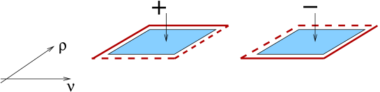
Figure 1: Plaquette update: A plaquette occupation number is changed by $+1$ (lhs. plot) or $-1$ (rhs.) and the fluxes at the links of the plaquette are changed simultaneously. We use a full line for an increase by +1 and a dashed line for a decrease by $-1$. The directions $1\leq\nu<\rho\leq 4$ indicate the plane of the plaquette.

The simplest local change is to increase or decrease a plaquette occupation number $p_{x,\nu\rho}$ by $\pm 1$ and to compensate the violation of the constraint on the links of the lattice by changing the link fluxes $l_{x,\sigma}$ by $\pm 1$. The two possible changes (one for increasing $p_{x,\nu\rho}$, one for decreasing) are illustrated in Fig. 1. The change of $p_{x,\nu\rho}$ by $\pm 1$ is indicated by the signs $+$ or $-$, while for the flux variables we use a dashed line to indicate a decrease by $-1$ and a full line for an increase by $+1$. It is easy to see that the pattern of changes for the flux variables not only compensates the violation of the link-based constraints from changing $p_{x,\nu\rho}$ but also leaves intact the site-based constraints at all four corners of the plaquette. We stress that for the case of gauge group Z₃ addition of $\pm 1$ is understood modulo 3, which is the usual addition, except for the cases $1+1=-1$ and $-1-1=1$.

A full sweep of these “plaquette updates” consists of visiting all plaquettes and offering one of the two changes of Fig. 1 with equal probability. The offer is accepted with the usual Metropolis probability $\min(1,{\cal W}^{\;\prime}_{loc}/{\cal W}_{loc})$ where ${\cal W}^{\;\prime}_{loc}$ and ${\cal W}_{loc}$ are the local weights of the trial configuration and the old configuration. They can easily be evaluated from the weight factors discussed in the previous section.

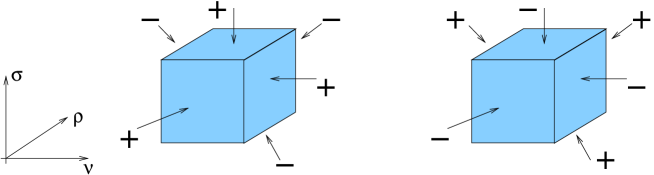
Figure 2: Cube update: The plaquette occupation numbers of a 3-cube are changed according to the two patterns we show. The edges of the 3-cube are parallel to the directions $1\leq\nu<\rho<\sigma\leq 4$.

It is easy to see that the plaquette update alone is ergodic. Nevertheless we found it advantageous to augment the plaquette update with a “cube update” that involves only changes of plaquette numbers $p_{x,\nu\rho}$. The cube update helps to decorrelate the system in parameter regions where link flux has a very small Boltzmann weight. The plaquettes on the faces of 3-cubes of our 4-D lattice are changed according to one of the two patterns shown in Fig. 2 (for Z₃ addition is again modulo 3). The two possibilities are offered with equal probability and it is easy to check that the link-based constraints are not violated, and since no flux variables are involved also the site-based constraints remain intact. A full sweep of cube updates consists of visiting all 3-cubes, offering one of the two changes and accepting them with the Metropolis probability computed from the local weight factors.

3.2 Surface worm algorithm

The surface worm algorithm (SWA) is constructed by breaking up the plaquette update discussed in the previous subsection into smaller building blocks used to grow filament-like clusters on which the flux and plaquette variables are changed. We will first discuss in detail the SWA for the Z₃ Gauge-Higgs model and then address the modifications necessary for U(1).

As for any worm algorithm, in the SWA the constraints are temporarily violated at a link $L_{V}$ and the two sites at its endpoints. This is done by changing the flux at a randomly chosen link by $\pm 1$ (addition is again modulo 3 for the Z₃ case). The defect at $L_{V}$ is then propagated through the lattice by offering steps where a plaquette occupation number is changed by $\pm 1$ and two flux variables at two of the links of the plaquette. We refer to these structures as “segments” and show some examples in Fig. 3. Attaching segments propagates the link $L_{V}$ where the constraint is violated through the lattice until the worm decides to terminate with the insertion of another unit of link flux. Each step is accepted with a Metropolis decision.

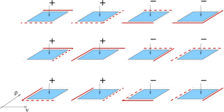
Figure 3: 12 of the 24 possible positive (marked with $+$) and negative segments in the $\nu$-$\rho$-plane ($\nu<\rho$). The remaining 12 segments are exactly the same but with the position of the empty and dotted links exchanged. Segments in other planes are constructed equivalently. The plaquette occupation numbers are changed as indicated by the signs. The links marked with full (dashed) lines are changed by $+1$ ($-1$). The empty link shows where the segment is attached to the worm and the dotted link is the new position of the link $L_{V}$ where the constraints are violated.

Fig. 3 shows some examples of segments that are used by the SWA. The plaquette occupation numbers are changed by $\pm 1$ as indicated and also the fluxes at two of the links of the plaquette (again we use a full line if the flux at a link is increased by $+1$ and dashed lines for a decrease by $-1$). We refer to a segment as a “positive segment” if the plaquette occupation number is increased (first and second segment shown in Fig. 3) and use “negative segment” otherwise (third and fourth segment). The empty link represents the link where a segment is attached to the existing filament-like structure of the SWA and the dotted link is the new (= shifted) position of the link $L_{V}$ where the constraints are violated (“head of the worm”).

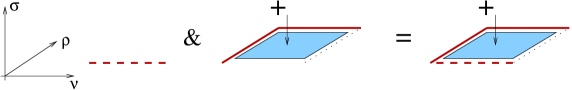
(a) The worm starts by decreasing the flux in $\nu$ direction. Subsequently it adds a segment in the $\nu$-$\rho$ plane.

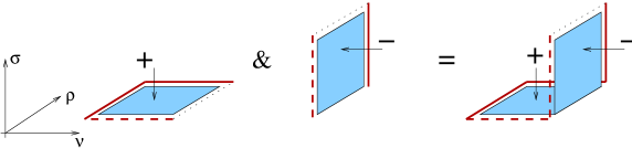
(b) The worm adds a segment in the $\rho$-$\sigma$ plane.

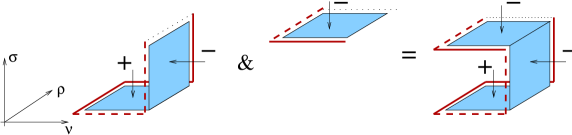
(c) The worm adds a segment in the $\nu$-$\rho$ plane.

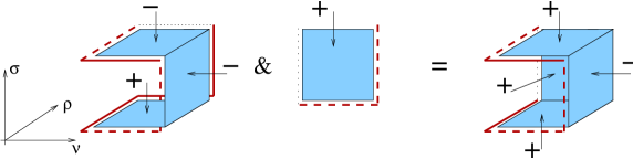
(d) A segment in the $\nu$-$\sigma$ plane is added.

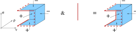
(e) The worm decides to saturate the violated constraint by adding a unit of flux in the $\sigma$ direction and terminates.

Figure 4: Example of a surface worm algorithm on an initially empty lattice.

Thus the SWA proceeds as follows (for an example see Figs. 4(a)–4(e)):

• The SWA starts at a randomly chosen link $L_{0}$ where the flux is changed by $\pm 1$ (in the example Fig. 4(a) the flux is changed by $-1$). At this link and at its endpoints the constraints are violated, i.e., $L_{V}=L_{0}$.

• Subsequently the SWA either moves $L_{V}$ by attaching a suitable segment (Figs. 4(a)–4(d)) or decides to change the link flux at $L_{V}$ to heal the violated constraint thus terminating the worm (Fig. 4(e)).

Whenever the worm decides to add a new segment it first randomly determines a new plane for the segment. This plane has to contain the direction of the link $L_{V}$ that currently violates the constraint. Subsequently the worm has to determine whether to insert a positive or a negative segment to create only admissible configurations. The following steps and Fig. 5 explain how the worm selects an admissible segment ($1\leq\nu<\rho<\sigma\leq 4$):

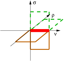
(a) $L_{V}\parallel\widehat{\nu}$

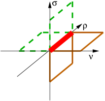
(b) $L_{V}\parallel\widehat{\rho}$

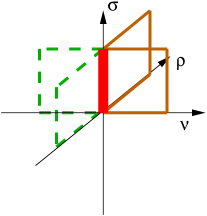
(c) $L_{V}\parallel\widehat{\sigma}$

Figure 5: This figure depicts the constraints of the dual partition function. It can be used to determine whether a positive or negative segment will be inserted by the worm: The link $L_{V}$ where the constraint is violated at the current step of the worm either points in $\nu$, $\rho$ or $\sigma$ direction (plots (a), (b) or (c)), and is marked by a fat link in the corresponding diagrams. Both the old and the new plaquette are attached to the link and need to be identified in the corresponding plot. If they both are surrounded by the same type of line (full versus dashed) the sign of the change of the plaquette variable remains the same, otherwise an extra factor ($-1$) is taken into account.

1. Depending on the direction of the link $L_{V}$ (i.e., $L_{V}\parallel\widehat{\nu}$, $L_{V}\parallel\widehat{\rho}$ or $L_{V}\parallel\widehat{\sigma}$) identify $L_{V}$ as the central link surrounded by four plaquettes in one of the diagrams of Fig. 5.

2. Identify the “old plane” and the “new plane”:
   Old plane: plane of the last successfully updated segment.
   New plane: plane of the new trial segment.

3. If the plaquettes in the old and the new plane are marked by different lines (full versus dashed) keep the same type of segment. Otherwise change the type of segment from positive to negative or vice-versa.

Note that when the worm attempts to revisit the last updated plaquette (i.e., it moves backwards) then the new and old planes coincide. Thus the segment changes and the last move of the worm is undone.

In addition to the example of Fig. 4, in Fig. 6 we show a short worm that generates the plaquette update of the local algorithm discussed in the previous subsection. We have already stressed that the plaquette update is ergodic and the SWA thus is ergodic too.

The pseudo-code listed below describes the algorithm. For the coordinates of plaquettes we use $P$, and $L$ for the coordinates of links. In particular the link where the constraints are violated (head of the worm) is denoted by $L_{V}$. By ${s}_{P}=(p_{P},l_{0},l_{1})$ we denote the current occupation numbers of a segment, i.e., the occupation number $p_{P}$ of the plaquette at $P$ and the two links fluxes $l_{0}$ and $l_{1}$ which are changed in the type of segment chosen (in the examples of segments shown in Fig. 3 $l_{0}$ and $l_{1}$ are the link fluxes marked by full or dashed lines). The variable $\Delta_{{s}}=(\delta_{p},\delta_{l_{0}},\delta_{l_{1}})$ denotes the change of the occupation numbers of ${s}_{P}$. Note that the sign of the change $\delta_{p}$ (“positive segment” versus “negative segment”) has to be chosen according to the rules stated in the discussion of Fig. 5. By $x\oplus y$ we denote the addition modulo 3 which is the usual addition operation except in the cases $+1\oplus+1=-1$ and $-1\oplus-1=+1$. By weight_ratio$(b\leftarrow a)$ we denote the ratio ${\cal W}_{loc}^{\;\prime}/{\cal W}_{loc}$ when changing an element $a$ into $b$. Here $a$ and $b$ are either a link flux before and after the change by $\pm 1$ or a full segment (a plaquette number $p_{P}$ and two link fluxes $l_{0},l_{1}$) before and after the respective changes. Finally, rand() is a random number generator for uniformly distributed real numbers in the interval $[0,1)$.

Pseudocode for surface worms: select a lattice link $L_{0}$ randomly

select $\delta_{l}\in\{-1,+1\}$ randomly

$l^{\prime}\,\longleftarrow\,l_{L}\,\oplus\,\delta_{l}$

if rand() $\leq\;$ weight_ratio($l^{\prime}\,\leftarrow\,l_{L}$)

$l_{L}\,\longleftarrow\,l^{\prime}$

$L_{V}\,\longleftarrow\,$ $L_{0}$

else

terminate worm

end if

repeat until worm is complete:

select a direction $\rho\in\{\pm\hat{1},\pm\hat{2},\pm\hat{3},\pm\hat{4}\}$

if $\widehat{\rho}\parallel L_{V}$ then

select $\delta_{l}$ such that the violated constraint at $L_{V}$ is healed

$l^{\prime}\,\longleftarrow\,l_{L_{V}}\,\oplus\,\delta_{l}$

if rand() $\leq\;$ weight_ratio($l^{\prime}\,\leftarrow\,l_{L_{V}}$)

$l_{L_{V}}\,\longleftarrow\,l^{\prime}$

terminate worm

end if

else

the plaquette $P$ for a new segment is spanned by $L_{V}$ and $\widehat{\rho}$

randomly select $L^{\prime}_{V}\neq L_{V}$ from the links bounding $P$

choose $\Delta_{{s}}$ such that the constraint at $L_{V}$ is healed

${s}^{\prime}\,\longleftarrow\,{s}_{P}\,\oplus\,\Delta_{{s}}$

if rand() $\leq\;$ weight_ratio(${s}^{\prime}\,\leftarrow\,{s}_{P}$)

${s}_{P}\,\longleftarrow\,{s}^{\prime}$

$L_{V}\,\longleftarrow L_{V}^{\prime}$

end if

end repeat until worm is complete

It is straightforward to show detailed balance using the Boltzmann weights and that the algorithm is ergodic.

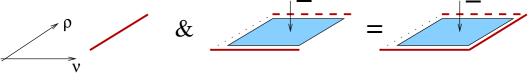
(a) The worm starts by increasing the flux in the $\nu$-direction and then adds a segment in the $\nu$-$\rho$ plane.

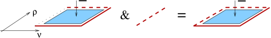
(b) The worm decides to saturate the violated constraint by decreasing the flux at $L_{V}$ by one unit and terminates.

Figure 6: Example how the worm generates the local plaquette update discussed in the previous subsection.

Modifications for the U(1) gauge-Higgs surface worm algorithm

From Eq.(3) and Eq.(9) we observe that the SWA has to be adapted in order to simulate the U(1) model:

• Due to the extra unconstrained set of link variables $\overline{l}_{x,\nu}$, for U(1) a full sweep consists of a worm sweep ($V_{4}=N_{s}^{3}N_{t}$ worms) to update the $l_{x,\nu}$ and $p_{x,\nu\rho}$ plus a conventional local Metropolis sweep to update all $\overline{l}_{x,\nu}$.

• To extend the range of the constrained variables to all integer numbers and enforce the total flux at every link and site to vanish, the operation $x\oplus y$ is replaced by a normal addition $x+y$. In the pseudo-code: ${s}_{P}\,\oplus\,\Delta_{{s}}$ is replaced by ${s}_{P}\ +\ \Delta_{{s}}$.

4 Assessment of the surface worm algorithm

4.1 Validity of the SWA

To evaluate the validity of the algorithm we will use several thermodynamical observables and their susceptibilities. For both models we study the first and second derivatives with respect to the inverse gauge coupling $\beta$, i.e., the plaquette expectation value and its susceptibility,

$$\langle U\rangle=\frac{1}{6N_{s}^{3}N_{t}}\frac{\partial}{\partial\beta}\ln\ Z\quad,\quad\chi_{U}=\frac{1}{6N_{s}^{3}N_{t}}\frac{\partial^{2}}{\partial\beta^{2}}\ln\ Z\ .$$ (12)

For the Z₃ case we also consider the particle number density $n$ and its susceptibility which are the derivatives with respect to the chemical potential,

$$n=\frac{1}{N_{s}^{3}N_{t}}\frac{\partial}{\partial\mu}\ln\ Z\quad,\quad\chi_{n}=\frac{1}{N_{s}^{3}N_{t}}\frac{\partial^{2}}{\partial\mu^{2}}\ln\ Z\ .$$ (13)

Finally, for the U(1) model we analyze the derivatives with respect to $\kappa$,

$$\langle|\phi|^{2}\rangle=\frac{1}{N_{s}^{3}N_{t}}\frac{\partial}{\partial\kappa}\ln\ Z\quad,\quad\chi_{|\phi|^{2}}=\frac{1}{N_{s}^{3}N_{t}}\frac{\partial^{2}}{\partial\kappa^{2}}\ln\ Z\ .$$ (14)

The correctness of the flux representation has already been established in [10, 11]. Thus here we can focus on the SWA. To check for correctness we compare the SWA results to the data coming from the local Metropolis algorithm (LMA) in the flux representation and for the cases where there is no sign problem also to results from a conventional approach in the standard representation.

For all simulations we used thermalization and decorrelation sweeps (see below for their numbers). For the SWA one sweep consists of $V_{4}=N_{s}^{3}N_{t}$ worms and for the case of U(1) also of a sweep through all unconstrained link variables $\overline{l}_{x,\nu}$. For the LMA a sweep is defined as a sequence of plaquette updates for all $6V_{4}$ plaquettes plus cube updates for all $4V_{4}$ cubes. For the U(1) model and the Z₃ case at $\mu=0$ we can also compare to the conventional approach where as usual a sweep is defined as applying one local Metropolis update to all degrees of freedom. All error bars we show were determined using a Jackknife analysis and are corrected with the factors from the respective autocorrelation times (see below).

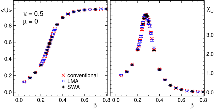
Figure 7: Z₃ model: $\langle U\rangle$ and $\chi_{U}$ at $\kappa=0.5$ and $\mu=0$ as a function of $\beta$ on a $10^{4}$ lattice. We compare the results of the SWA (asterisks) to the LMA (circles) and the conventional approach (crosses).

For the Z₃ model we compared simulations for several parameter sets and found very good agreement of the results from the different approaches. As examples we show results for two parameter sets: 1) The behavior across a crossover transition as a function of $\beta$ at $\kappa=0.5$ and $\mu=0$ (no complex action problem) on a $10^{4}$ lattice (Fig. 7). 2) The behavior across a first order transition as a function of $\mu$ at $\kappa=0.1$ and $\beta=0.6$ on a $8^{3}\times 50$ lattice (Fig. 8). In the latter case the standard representation has a complex action problem and we only can compare the results from SWA and LMA. For both tests we used $10^{6}$ equilibration sweeps and $10^{6}$ measurements separated by $10$ sweeps for decorrelation.

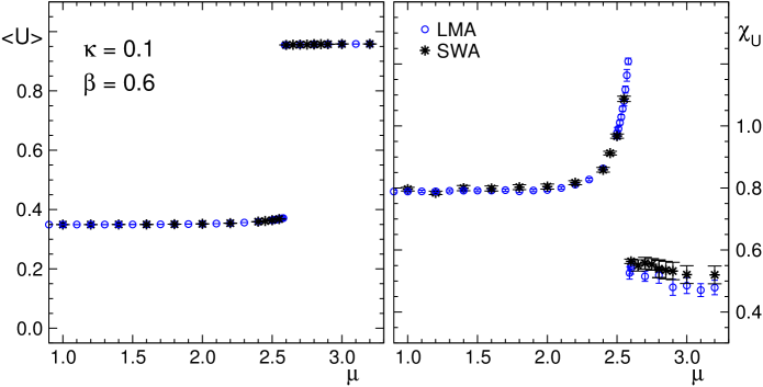
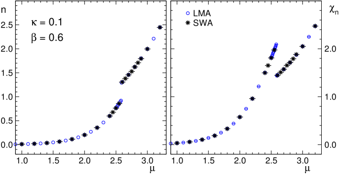
Figure 8: Z₃ model: The observables $\langle U\rangle$, $\chi_{U}$, $n$ and $\chi_{n}$ as a function of $\mu$ at $\kappa=0.1$ and $\beta=0.6$ on a $8^{3}\times 50$ lattice. We compare the results from the SWA (asterisks) and the LMA (circles).

Similarly we also confirmed the correctness of the SWA in the U(1) model checking the agreement of all three approaches at different parameters and lattice sizes. As an example, Fig. 9 shows the results obtained with the LMA (crosses), with the SWA (circles) and the conventional approach (asterisks) at $\lambda=1$ and $\kappa=$ $5$, $8$ and $9$ on a $10^{4}$ lattice. For this test we used $10^{5}$ equilibration sweeps and $10^{5}$ measurements separated by $10$ sweeps for decorrelation. As for the Z₃ case we find very good agreement among the different approaches thus establishing the correctness of the SWA also for the U(1) model.

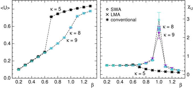
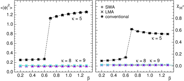
Figure 9: U(1) model: Observables as a function of $\beta$ at $\lambda=1.0$ for $\kappa=5,8$ and 9 on a $10^{4}$ lattice. We compare results from three algorithms: The conventional approach (asterisks), the SWA (circles) and the LMA (crosses).

4.2 Characteristic quantities of the algorithms

For a meaningful comparison of the performance and autocorrelation times of the SWA and LMA algorithms we study suitable characteristic quantities in order to describe the behavior of both algorithms in different regions of the parameter space. The definitions are patterned after related quantities introduced for the analysis of worm algorithms with open ends [7].

• Plaquette changes ${\cal P}$:

  $${\cal P}=\mbox{average number of plaquettes changed per update}$$

• Starting fraction ${\cal S}$:

  $${\cal S}=\frac{\mbox{number of successful update starts}}{\mbox{number of all start attempts}}\;\leq\;1$$

• Cost ratio ${\cal C}$:

  $${\cal C}=\frac{\mbox{number of attempted changes (plaquettes and links)}}{\mbox{number of accepted changes}}\;\geq\;1$$

In these definitions ”update” refers to one surface worm for the SWA case. For the LMA it is the average of a plaquette and a cube update which we consider in a mix of 6$V_{4}$ plaquette updates and 4$V_{4}$ cube updates per LMA sweep (see above). From the definition of these characteristic quantities it is obvious that an optimal algorithm is characterized by a large value of ${\cal P}$ and values of ${\cal S}$ and ${\cal R}$ close to 1.

In Table 1 we show the characteristic quantities for the SWA and LMA algorithms in the Z₃ case. We compare three different sets of parameters denoted by Z-1, Z-2 and Z-3 (see the first column for the corresponding parameter values) and four different volumes (second column). The parameters of Z-1 are located below the condensation transition shown in Fig. 8, the set Z-2 is in the condensed phase (compare Fig. 11 from [10]) and the set Z-3 is inside the crossover region of Fig. 7.

Table 1 demonstrates that the SWA has a larger probability for starting an update than the LMA (${\cal S}_{SWA}>{\cal S}_{LMA}$ for all data sets and volumes). Furthermore the cost ratio ${\cal R}$ of the SWA is smaller or equal (equal only for the set Z-2) to the LMA case. These two quantities indicate that the SWA is more effective than the LMA. The observation that ${\cal P}$ is larger for the LMA is mainly due to the fact that an accepted cube update of the LMA changes 6 plaquettes (although at the cost of a low acceptance rate). It is interesting to note that the values for the characteristic quantities are essentially independent of the volume.

Table 2 collects the data for the U(1) case. Here we consider three different sets of parameters U-1, U-2, U-3 (first column) on four different volumes (second column). The set U-2 is located very close to the transition shown in Fig. 9, the set U-1 is below and the set U-3 above the transition.

The general behavior for the characteristic quantities is essentially the same as in the Z₃ case: For all sets the starting probability of the SWA is larger than that of the LMA, and also the cost efficiency is considerably better for the SWA. As in the Z₃ case we find that the average number of updated plaquettes ${\cal P}$ is larger for the LMA, which also here is due to the cube updates, which, however, have a much lower acceptance rate as is obvious from ${\cal S}$ and ${\cal C}$. The difference in the characteristic quantities between the $4^{4}$ and larger volumes for the set U-2 is due to finite-size effects: In the smallest volume the transition is rounded and slightly shifted towards smaller values of $\beta$, such that for the smallest volume the parameters we work at are further remote from the transition and both algorithms are more efficient.

Parameters	$V$	${\cal S}_{SWA}$	${\cal P}_{SWA}$	${\cal C}_{SWA}$	${\cal S}_{LMA}$	${\cal P}_{LMA}$	${\cal C}_{LMA}$
Set: Z-1	$4^{3}\times 50$	0.203	0.095	6.892	2.9e-3	4.456	320.7
$\kappa=0.1,$	$8^{3}\times 50$	0.203	0.095	6.892	2.9e-3	4.455	320.7
$\beta=0.6,$	$12^{3}\times 50$	0.203	0.095	6.892	2.9e-3	4.455	320.7
$\mu=2.0$	$16^{3}\times 50$	0.203	0.095	6.892	2.9e-3	4.455	320.7
Set: Z-2	$4^{3}\times 50$	0.245	1.196	5.319	0.172	5.384	5.346
$\kappa=0.1,$	$8^{3}\times 50$	0.244	1.186	5.431	0.172	5.384	5.346
$\beta=0.8,$	$12^{3}\times 50$	0.245	1.199	5.320	0.172	5.384	5.346
$\mu=1.6$	$16^{3}\times 50$	0.244	1.187	5.425	0.172	5.384	5.346
Set: Z-3	$4^{4}$	0.697	0.802	3.081	0.098	1.286	10.88
$\kappa=0.5,$	$8^{4}$	0.698	0.802	3.081	0.098	1.286	10.88
$\beta=0.28,$	$12^{4}$	0.698	0.802	3.081	0.098	1.286	10.88
$\mu=0.0$	$16^{4}$	0.697	0.802	3.081	0.098	1.286	10.88

Table 1: Characteristic quantities for the Z₃ model (see the text for their definitions). We used $10^{6}$ steps for equilibration and $10^{6}$ measurements separated by $2$ steps for decorrelation. The errors are smaller than the last digit we show.

Parameters	$V$	${\cal S}_{SWA}$	${\cal P}_{SWA}$	${\cal C}_{SWA}$	${\cal S}_{LMA}$	${\cal P}_{LMA}$	${\cal C}_{LMA}$
Set : U-1	$4^{4}$	0.201	0.085	6.899	1.2e-3	1.277	904.6
$\kappa=5,$	$8^{4}$	0.201	0.085	6.902	1.2e-3	1.278	909.2
$\lambda=1,$	$12^{4}$	0.201	0.085	6.902	1.2e-3	1.278	909.4
$\beta=0.40$	$16^{4}$	0.201	0.085	6.902	1.2e-3	1.278	909.4
Set: U-2	$4^{4}$	0.681	1.275	3.310	0.167	1.813	6.263
$\kappa=5,$	$8^{4}$	0.220	0.199	6.124	4.6e-3	2.243	224.3
$\lambda=1,$	$12^{4}$	0.220	0.198	6.124	4.6e-3	2.243	224.3
$\beta=0.65$	$16^{4}$	0.220	0.198	6.124	4.6e-3	2.243	224.3
Set: U-3	$4^{4}$	0.107	0.100	8.775	0.061	5.962	14.82
$\kappa=8,$	$8^{4}$	0.107	0.100	8.773	0.061	5.962	14.92
$\lambda=1,$	$12^{4}$	0.107	0.100	8.774	0.060	5.962	14.91
$\beta=1.10$	$16^{4}$	0.107	0.101	8.766	0.060	5.962	14.91

Table 2: Characteristic quantities for the U(1) model (see the text for their definitions). We used $10^{6}$ steps for equilibration and $10^{6}$ measurements separated by $2$ steps for decorrelation. The errors are smaller than the last digit we show.

Finally, comparing $R_{SWA}$ and $S_{SWA}$ for both the Z₃ and U(1) cases, we observe that even though many worms start successfully, not all of them create non-trivial changes, i.e., there is a sizable probability that in the second step a worm reverts its initial step. This is also reflected in Fig. 10 where we show the abundance distribution of the worms as a function of their length $l$ defined as the number of segments of a worm. The distribution decreases roughly exponentially with $l$. However, as we shall see in the next subsection, a few long worms are enough to have a very efficient sampling.

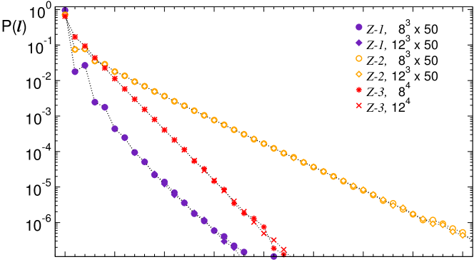
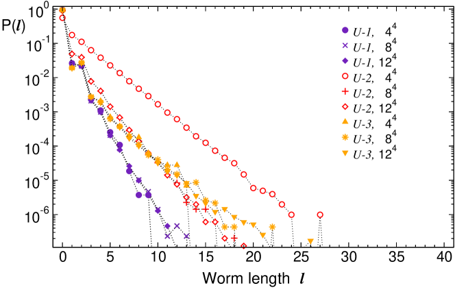
Figure 10: Normalized histograms of the worm length for the Z₃ model (upper plot) and the U(1) model (lower plot).

4.3 Autocorrelation times

In this subsection we analyze the integrated autocorrelation time $\tau_{int}^{O}$ of several observables $O$ in both models. Since we are comparing two different algorithms we normalize the autocorrelation times as in [7]: define one sweep as $\tau_{0}=6V_{4}/{\cal P}$ configurations, i.e., the average number of attempts needed to change every plaquette of the lattice as the unit for the integrated autocorrelation times $\tau_{int}^{O}$. In units of updates we have $\tau_{0}=6V_{4}/({\cal P}\,N_{updates})$, where $N_{updates}$ is defined as either $V_{4}$ worms for the SWA or $6V_{4}$ plaquette updates plus $4V_{4}$ cube updates for the LMA, i.e., a total of $10V_{4}$ local updates.

In order to obtain a measure for the computational effort, the results are multiplied by the cost ratio ${\cal C}$. In other words we show $\overline{\tau}_{int}={\cal C}\,\tau_{int}/\tau_{0}$, where $\tau_{int}$ simply is the unnormalized autocorrelation time in units of updates. The statistical errors of autocorrelation times were estimated with a jackknife analysis and were found at the 10 percent level for the statistics at our disposal. This is sufficient for the subsequent comparison of the two algorithms.

For the autocorrelation analysis we use the same sets and volumes as for the discussion of the characteristic quantities of the SWA and the LMA in the previous subsection. Table 4 shows the autocorrelation times in the Z₃ case for the SWA and Table 4 is for the LMA. Similarly, Tables 6 and 6 correspond to the U(1) case.

Parameters	$V$	$\overline{\tau}^{U}_{int}$	$\overline{\tau}^{\chi_{U}}_{int}$	$\overline{\tau}^{n}_{int}$	$\overline{\tau}^{\chi_{n}}_{int}$
Set: Z-1	$4^{3}\times 50$	180	97	0.9	0.6
$\kappa=0.1,$	$8^{3}\times 50$	200	90	1.0	0.6
$\beta=0.6,$	$12^{3}\times 50$	200	92	1.0	0.6
$\mu=2.0$	$16^{3}\times 50$	200	88	1.3	0.8
Set: Z-2	$4^{3}\times 50$	81	36	25	13
$\kappa=0.1,$	$8^{3}\times 50$	84	32	25	14
$\beta=0.8,$	$12^{3}\times 50$	$>$ 83	38	27	12
$\mu=1.6$	$16^{3}\times 50$	$>$ 90	37	30	13
Set: Z-3	$4^{4}$	2.5	1.3	0.3	0.2
$\kappa=0.5,$	$8^{4}$	5.4	2.9	0.6	0.4
$\beta=0.28,$	$12^{4}$	6.0	3.1	0.6	0.5
$\mu=0.0$	$16^{4}$	7.7	3.2	0.7	0.5

Table 3: Z₃ model: SWA autocorrelation times for different parameter sets.

Parameters	$V$	$\overline{\tau}^{U}_{int}$	$\overline{\tau}^{\chi_{U}}_{int}$	$\overline{\tau}^{n}_{int}$	$\overline{\tau}^{\chi_{n}}_{int}$
Set: Z-1	$4^{3}\times 50$	5400	2900	5600	3100
$\kappa=0.1,$	$8^{3}\times 50$	5800	3000	5900	3200
$\beta=0.6,$	$12^{3}\times 50$	5400	3000	6100	4200
$\mu=2.0$	$16^{3}\times 50$	5400	3000	$>$7800	4300
Set: Z-2	$4^{3}\times 50$	67	48	750	310
$\kappa=0.1,$	$8^{3}\times 50$	68	51	760	300
$\beta=0.8,$	$12^{3}\times 50$	70	49	600	350
$\mu=1.6$	$16^{3}\times 50$	71	46	600	340
Set: Z-3	$4^{4}$	110	55	59	23
$\kappa=0.5,$	$8^{4}$	110	66	65	24
$\beta=0.28,$	$12^{4}$	120	69	67	25
$\mu=0.0$	$16^{4}$	130	73	67	27

Table 4: Z₃ model: LMA autocorrelation times for different parameter sets.

First, we observe that the autocorrelation times for the set close to the first order transition (set U-2) increase with the volume, while the others are essentially volume independent. It is also interesting to look at the sets Z-2 and U-3, where ${\cal P}_{LMA}$ approaches 6 (see Tables 1 and 2), i.e., the configuration space is dominated by closed surfaces, since boundary flux is costly for these parameter sets. On the one hand, $\overline{\tau}_{int}^{U}$ and $\overline{\tau}_{int}^{\chi_{U}}$ are larger for the worm algorithm, which is due to the fact that the worm updates links in every move, so if the Boltzmann weight of the link variables is very low then most of the worms have only a few segments (see Fig. 10). On the other hand $\overline{\tau}_{int}$ of the observables that depend only on the link occupation number is much smaller for the SWA, a fact which reflects the very low acceptance rate of the plaquette update of the LMA.

Parameters	$V$	$\overline{\tau}^{U}_{int}$	$\overline{\tau}^{\chi_{U}}_{int}$	$\overline{\tau}^{|\phi|^{2}}_{int}$	$\overline{\tau}^{\chi_{|\phi|^{2}}}_{int}$
Set: U-1	$4^{4}$	2.2	3.1	0.6	0.3
$\kappa=5,$	$8^{4}$	2.3	1.6	0.5	0.3
$\lambda=1,$	$12^{4}$	2.4	1.5	0.6	0.3
$\beta=0.40$	$16^{4}$	2.6	1.1	0.5	0.4
Set: U-2	$4^{4}$	5.7	3.5	9.5	3.9
$\kappa=5,$	$8^{4}$	12	6.9	2.9	1.2
$\lambda=1,$	$12^{4}$	19	7.8	3.3	1.4
$\beta=0.65$	$16^{4}$	21	7.9	3.1	1.6
Set: U-3	$4^{4}$	1600	870	1.1	0.9
$\kappa=8,$	$8^{4}$	1700	840	1.2	1.0
$\lambda=1,$	$12^{4}$	$>$1600	740	1.8	0.9
$\beta=1.10$	$16^{4}$	$>$1700	800	2.2	1.1

Table 5: U(1) model: SWA autocorrelation times for different parameters. We attribute the $V=4^{4}$ value $\overline{\tau}^{\chi_{U}}_{int}=3.1$, which is slightly higher than naively expected, to a finite volume effect caused by closed surfaces that wind around the rather short (4 lattice points) compact directions.

Parameters	$V$	$\overline{\tau}^{U}_{int}$	$\overline{\tau}^{\chi_{U}}_{int}$	$\overline{\tau}^{|\phi|^{2}}_{int}$	$\overline{\tau}^{\chi_{|\phi|^{2}}}_{int}$
Set: U-1	$4^{4}$	5800	2900	8100	4500
$\kappa=5,$	$8^{4}$	5800	3000	8600	4500
$\lambda=1.0,$	$12^{4}$	6100	4100	7400	5000
$\beta=0.4$	$16^{4}$	6200	4200	9100	5000
Set: U-2	$4^{4}$	71	48	180	93
$\kappa=5,$	$8^{4}$	4700	2600	7100	4100
$\lambda=1.0,$	$12^{4}$	7200	2800	8700	4300
$\beta=0.65$	$16^{4}$	7300	2800	9400	5000
Set: U-3	$4^{4}$	460	280	440	300
$\kappa=8,$	$8^{4}$	430	300	480	300
$\lambda=1,$	$12^{4}$	690	290	450	270
$\beta=1.10$	$16^{4}$	710	280	490	270

Table 6: U(1) model: LMA autocorrelation times for different parameters.

In general, comparing the results of both algorithms for the two different models, we can conclude that the SWA outperforms the LMA for a large range of parameters. Only in the region of the space of couplings where the link weight is very large the worm algorithm has difficulties to sample the system efficiently, a problem which can easily be overcome with extra cube sweeps or by adding a worm with only plaquettes suggested in [4].

5 Summary

In this article we present a generalization of the worm algorithm to systems that are described by surfaces with boundaries of flux, i.e., abelian Gauge-Higgs systems. Rewriting the standard form of abelian Gauge-Higgs systems in terms of surfaces and fluxes (dual representation) overcomes the complex action problem at finite chemical potential. We study Gauge-Higgs systems with two gauge groups Z₃ and U(1). For the Z₃ case a chemical potential can be coupled and the system has a complex action problem.

The key idea of our newly developed surface worm algorithm (SWA) is to build up filament-like structures where the dual degrees of freedom are changed by adding segments built from plaquette variables and two lines of matter flux. We compare the SWA to a local Metropolis algorithm (LMA) for the dual representation and in the cases without a sign problem also to a conventional Monte Carlo simulation in the standard approach. The comparison is used to establish the correctness of the SWA in several simulations at different parameter values.

To study the performance of the SWA we analyze characteristic quantities: the starting probability, the number of updated plaquettes and the cost efficiency. Based on these characteristic quantities we conclude that for both gauge groups and most parameter values the SWA is considerably more efficient than the LMA. This finding is confirmed by an analysis of autocorrelation times where again the SWA is found to decorrelate faster (partly considerably faster) than the LMA.

We expect that the generalization of the worm concept to surface-type degrees of freedom will contribute to developing new tools for systems with gauge interactions in a dual language. Another important aspect is that models where the complex action problem is solved may serve as reference systems for testing other approaches such as various reweighting and expansion techniques.

Appendix: Dual representation for the U(1) Gauge-Higgs system

In this appendix we summarize a brief derivation of the dual representation of the U(1) Gauge-Higgs system we use in this article. The gauge action $S_{G}$ is given by (1) with U(1) valued link variables $U_{x,\nu}$. The action $S_{M}$ for the matter field is (8). The partition sum $Z$ is obtained by integrating the Boltzmann factor $e^{-S_{G}-S_{M}}$ over all field configurations, $Z=\int D[U]D[\phi]e^{-S_{G}-S_{M}}$. For the Higgs field the measure is a product over all lattice points $x$, and we use polar coordinates $\phi_{x}=r_{x}e^{i\theta_{x}}$ for integrating each $\phi_{x}$ in the complex plane. The U(1) gauge variables $U_{x,\nu}=e^{i\varphi_{x,\nu}}$ at each link are integrated over the unit circle such that the path integral reads

$$Z=\int\!\!D[U]D[\phi]\,e^{-S_{G}-S_{M}}=\left(\prod_{x,\nu}\!\int_{-\pi}^{\pi}\!\!\frac{d\varphi_{x,\nu}}{2\pi}\!\!\right)\!\!\left(\!\prod_{x}\!\int_{-\pi}^{\pi}\!\!\frac{d\theta_{x,\nu}}{2\pi}\!\!\int_{0}^{\infty}\!\!\!dr_{x}\,r_{x}\!\!\right)\!e^{-S_{G}-S_{H}}.$$ (15)

The normalization with $2\pi$ will be useful later.

The first step to obtain the representation of the full partition sum in terms of loops is to consider the Higgs part of the problem. For that purpose we define the partition sum of the Higgs system in a gauge background as

$$Z_{H}=\int\!\!D[\phi]e^{-S_{M}}=\int\!\!D[\phi]\!\left(\prod_{x,\nu}e^{\phi_{x}^{\star}U_{x,\nu}\phi_{x+\widehat{\nu}}}e^{\phi_{x}U_{x,\nu}^{\star}\phi_{x+\widehat{\nu}}^{\star}}\!\right)\!\!\left(\prod_{x}B(|\phi_{x}|^{2})\!\right),$$ (16)

where we have slightly reorganized the nearest neighbor terms and write the corresponding sums in the exponent as a product of exponentials. The mass- and $\phi^{4}$-terms are taken into account in $B(r^{2})=\exp(-\kappa r^{2}-\lambda r^{4})$.

The next step is an expansion of the Boltzmann factors for the nearest neighbor terms (use $U_{x,\nu}^{\;\;\star}=U_{x,\nu}^{\;\;-1}$):

$$\prod_{x,\nu}\exp\!\left(\phi_{x}^{\star}U_{x,\nu}\phi_{x+\widehat{\nu}}\right)\exp\!\left(\phi_{x}U_{x,\nu}^{\star}\phi_{x+\widehat{\nu}}^{\star}\right)=$$ (17)

$$\sum_{\{n,\overline{n}\}}\!\!\left(\prod_{x,\nu}\!\frac{U_{x,\nu}^{\;\;n_{x,\nu}}\,{U_{x,\nu}^{\star}}^{\overline{n}_{x,\nu}}}{n_{x,\nu}!\,\overline{n}_{x,\nu}!}\right)\!\left(\prod_{x,\nu}\!\Big{(}\phi_{x}^{\star}\phi_{x+\widehat{\nu}}\Big{)}^{n_{x,\nu}}\,\Big{(}\phi_{x}\phi_{x+\widehat{\nu}}^{\star}\Big{)}^{\overline{n}_{x,\nu}}\!\right)\!=$$

$$\sum_{\{n,\overline{n}\}}\!\!\left(\prod_{x,\nu}\!\frac{U_{x,\nu}^{\;\;n_{x,\nu}-\overline{n}_{x,\nu}}}{n_{x,\nu}!\,\overline{n}_{x,\nu}!}\right)\left(\!{\phi_{x}^{\,\star}}^{\sum_{\nu}[n_{x,\nu}+\overline{n}_{x-\widehat{\nu},\nu}]}\,{\phi_{x}}^{\sum_{\nu}[\overline{n}_{x,\nu}+n_{x-\widehat{\nu},\nu}]}\right),$$

where the expansion variables $n_{x,\nu}$ and $\overline{n}_{x,\nu}$ are non-negative integers attached to the links of the lattice. By $\sum_{\{n,\overline{n}\}}$ we denote the sum over all configurations of the expansion variables $n_{x,\nu},\overline{n}_{x,\nu}\in[0,\infty)$. The partition sum of the Higgs field now reads

$$Z_{H} \!\!\!=\!\!\! \!\!\sum_{\{n,\overline{n}\}}\!\!\left(\prod_{x,\nu}\!\frac{U_{x,\nu}^{\;\;n_{x,\nu}-\overline{n}_{x,\nu}}}{n_{x,\nu}!\,\overline{n}_{x,\nu}!}\right)\!\!\left(\!\prod_{x}\int_{-\pi}^{\pi}\frac{d\theta_{x}}{2\pi}e^{-i\theta_{x}\sum_{\nu}[n_{x,\nu}-\overline{n}_{x,\nu}-(n_{x-\widehat{\nu},\nu}-\overline{n}_{x-\widehat{\nu},\nu})]}\!\right)$$ (18)

$$\hskip 28.45274pt\times\left(\prod_{x}\int_{0}^{\infty}\!\!\!dr_{x}\;r_{x}^{1+\sum_{\nu}[n_{x,\nu}+n_{x-\widehat{\nu},\nu}+\overline{n}_{x,\nu}+\overline{n}_{x-\widehat{\nu},\nu}]}\;B\big{(}r_{x}^{2}\big{)}\right)\!.$$

The integrals over the phase give rise to Kronecker deltas, which for notational convenience here we write as $\delta(n)$. The integrals over the modulus we abbreviate as

$$P(n)\;=\;\int_{0}^{\infty}dr\,r^{n+1}\,B\big{(}r^{2})\;=\;\int_{0}^{\infty}dr\,r^{n+1}\,e^{-\kappa r^{2}-\lambda r^{4}}\;.$$ (19)

They can easily be computed numerically. The Higgs field partition sum now reads:

$$Z_{H}\!\! \!\!=\!\! \!\!\sum_{\{n,\overline{n}\}}\!\!\left(\prod_{x,\nu}\!\frac{U_{x,\nu}^{\;\;n_{x,\nu}-\overline{n}_{x,\nu}}}{n_{x,\nu}!\,\overline{n}_{x,\nu}!}\right)\!\!\left(\!\prod_{x}\delta\!\left(\sum_{\nu}\big{[}n_{x,\nu}-\overline{n}_{x,\nu}-(n_{x-\widehat{\nu},\nu}-\overline{n}_{x-\widehat{\nu},\nu})\big{]}\!\right)\!\right)$$ (20)

$$\hskip 28.45274pt\times\left(\!\prod_{x}P\!\left(\sum_{\nu}\big{[}n_{x,\nu}+\overline{n}_{x,\nu}+n_{x-\widehat{\nu},\nu}+\overline{n}_{x-\widehat{\nu},\nu}\big{]}\right)\right)\!.$$

In this form the Higgs fields are completely eliminated and the partition sum is a sum over configurations of the $n$ and $\overline{n}$. The allowed configurations of the $n$ and $\overline{n}$ are subject to local constraints at each site $x$ enforced by the Kronecker deltas, i.e., at each site $x$ the variables must obey $\sum_{\nu}[n_{x,\nu}-\overline{n}_{x,\nu}-(n_{x-\widehat{\nu},\nu}-\overline{n}_{x-\widehat{\nu},\nu})]=0$.

In the current representation the constraints mix both the $n$ and the $\overline{n}$ variables. The structure of the constraints can be simplified by introducing new variables $l_{x,\nu}\in(-\infty,\infty)$ and $\overline{l}_{x,\nu}\in[0,\infty)$. They are related to the old variables by

$$n_{x,\nu}-\overline{n}_{x,\nu}=l_{x,\nu}\qquad\mbox{and}\qquad n_{x,\nu}+\overline{n}_{x,\nu}=|l_{x,\nu}|+2\overline{l}_{x,\nu}\;,$$ (21)

and the sum over all configurations of the $n,\overline{n}$ variables can be replaced by a sum over $l$- and $\overline{l}$-configurations. The partition sum turns into

$$Z_{H} \!\!=\!\! \sum_{\{l,\overline{l}\}}\left(\prod_{x,\nu}\!\frac{U_{x,\nu}^{\;\;l_{x,\nu}}}{(|l_{x,\nu}|+\overline{l}_{x,\nu})!\,\overline{l}_{x,\nu}!}\right)\!\!\left(\!\prod_{x}\delta\left(\sum_{\nu}\big{[}l_{x,\nu}-l_{x-\widehat{\nu},\nu}\big{]}\!\right)\right)$$ (22)

$$\hskip 28.45274pt\times\left(\!\prod_{x}P\!\!\left(\sum_{\nu}\big{[}|l_{x,\nu}|+|l_{x-\widehat{\nu},\nu}|+2(\overline{l}_{x,\nu}+\overline{l}_{x-\widehat{\nu},\nu})\big{]}\right)\right)\!.$$

In the final form (22) of the Higgs field partition sum, which we now refer to as dual representation, the constraints no longer mix the two types of flux variables. Obviously only the $l$-fluxes are subject to conservation of flux at each site $x$, i.e., only they must obey $\sum_{\nu}[l_{x,\nu}-l_{x-\widehat{\nu},\nu}]=0$ for all $x$.

Having mapped the Higgs field partition sum to the flux form (22) we now apply similar steps to the gauge fields to obtain the dual representation of the full partition sum (15). We write the full partition sum as $Z=\int D[U]e^{-S_{G}}Z_{H}$ and find

$$Z = \sum_{\{l,\overline{l}\}}\left(\prod_{x,\nu}\!\frac{1}{(|l_{x,\nu}|+\overline{l}_{x,\nu})!\,\overline{l}_{x,\nu}!}\right)\!\!\left(\!\prod_{x}\delta\left(\sum_{\nu}\big{[}l_{x,\nu}-l_{x-\widehat{\nu},\nu}\big{]}\!\right)\!\right)$$ (23)

$$\times\left(\!\prod_{x}P\!\left(\sum_{\nu}\big{[}|l_{x,\nu}|+|l_{x-\widehat{\nu},\nu}|+2(\overline{l}_{x,\nu}+\overline{l}_{x-\widehat{\nu},\nu})\big{]}\!\right)\!\right)Z_{G}[l]\,,$$

where we have interchanged the sum over the flux configurations and the integral over the gauge fields. The gauge field partition sum with link insertions according to a flux configuration $l$ is defined as

$$Z_{G}[l]=\int D[U]e^{-S_{G}}\,\prod_{x,\nu}\!U_{x,\nu}^{\;\;l_{x,\nu}}\;.$$ (24)

The gauge action $S_{G}$ as defined in (1) is a sum over plaquettes. We thus may write the Boltzmann factor $e^{-S_{G}}$ as a product over plaquettes and, as done for the Higgs field, we expand the corresponding exponentials into power series:

$$\prod_{x,\sigma<\tau}\!\!e^{\frac{\beta}{2}U_{x,\sigma\tau}}\,e^{\frac{\beta}{2}U_{x,\sigma\tau}^{\star}} \!\!\!=\!\!\! \sum_{\{m,\overline{m}\}}\!\left(\prod_{x,\sigma<\tau}\!\frac{(\frac{\beta}{2})^{m_{x,\sigma\tau}+\overline{m}_{x,\sigma\tau}}}{m_{x,\sigma\tau}!\,\overline{m}_{x,\sigma\tau}!}{U_{x,\sigma\tau}}^{m_{x,\sigma\tau}}\;{U_{x,\sigma\tau}^{\star}}^{\overline{m}_{x,\sigma\tau}}\right)$$

$$\!\!\!=\!\!\! \sum_{\{m,\overline{m}\}}\!\left(\prod_{x,\sigma<\tau}\!\frac{(\frac{\beta}{2})^{m_{x,\sigma\tau}+\overline{m}_{x,\sigma\tau}}}{m_{x,\sigma\tau}!\,\overline{m}_{x,\sigma\tau}!}\,\right)$$

$$\!\!\!\times\!\!\! \left(\prod_{x,\nu}{\,U_{x,\nu}}^{\sum_{\nu<\alpha}\big{[}p_{x,\nu\alpha}-p_{x-\widehat{\alpha},\nu\alpha}\big{]}-\sum_{\alpha<\nu}\big{[}p_{x,\alpha\nu}-p_{x-\widehat{\alpha},\alpha\nu}\big{]}}\!\right).$$

We introduced the expansion variables $m_{x,\sigma\tau},\overline{m}_{x,\sigma\tau}\in[0,\infty)$ attached to the plaquettes, and by $\sum_{\{m,\overline{m}\}}$ we denote the sum over all configurations of the expansion variables. In the second step we inserted the explicit expressions for the plaquettes in terms of the link variables, i.e., $U_{x,\sigma\tau}=U_{x,\sigma}U_{x+\widehat{\sigma},\tau}U_{x+\widehat{\tau},\sigma}^{\star}U_{x,\tau}^{\star}$, and reorganized the product over powers of links variables. Here we already introduced $m_{x,\nu\alpha}-\overline{m}_{x,\nu\alpha}=p_{x,\nu\alpha}$. This combination of the expansion variables plays the same role as the transformutation (21) used in the Higgs case for the simplification of the constraints. Exactly the same step is now implemented here: We promote $p_{x,\nu\alpha}\in(-\infty,\infty)$ into new dynamical variables, which together with another set of variables, $q_{x,\nu\alpha}\in[0,\infty)$, gives the final set of variables we use for the gauge fields. The $p$ and $q$ variables are related to the $m$ and $\overline{m}$ variables via (compare (21))

$$m_{x,\nu\alpha}-\overline{m}_{x,\nu\alpha}=p_{x,\nu\alpha}\quad\;\mbox{and}\quad\;m_{x,\nu\alpha}+\overline{m}_{x,\nu\alpha}=|p_{x,\nu\alpha}|+2q_{x,\nu\alpha}\;.$$ (26)

We will refer to the variables $p$ as plaquette occupation numbers or simply plaquette variables. Using the new variables (26) and inserting the expanded Boltzmann factor (Appendix: Dual representation for the U(1) Gauge-Higgs system) back into (24) we find

$$Z_{G}[l] \!\!=\!\! \sum_{\{p,q\}}\left(\prod_{x,\sigma<\tau}\frac{(\frac{\beta}{2})^{|p_{x,\sigma\tau}|+2q_{x,\sigma\tau}}}{(|p_{x,\sigma\tau}|+q_{x,\sigma\tau})!\,q_{x,\sigma\tau}!}\right)$$

$$\!\!\times\!\! \!\!\!\!\left(\!\prod_{x,\nu}\int_{-\pi}^{\pi}\!\!\frac{d\varphi_{x,\nu}}{2\pi}e^{i\varphi_{x,\nu}\left(\sum_{\nu<\alpha}\!\big{[}p_{x,\nu\alpha}-p_{x-\widehat{\alpha},\nu\alpha}\big{]}-\sum_{\alpha<\nu}\!\big{[}p_{x,\alpha\nu}-p_{x-\widehat{\alpha},\alpha\nu}\big{]}+l_{x,\nu}\right)}\!\!\right)\!\!.$$

The integrals in the last product are again representations of Kronecker deltas and give rise to constraints that are located at the links of the lattice. The summations over the variables $q_{x,\sigma\tau}$ can be done in closed form using the well known series representation of the modified Bessel functions

$$\sum_{q=0}^{\infty}\frac{(\frac{\beta}{2})^{|p|+2q}}{(|p|+q)!\,q!}\;=\;I_{|p|}(\beta)\;=\;I_{p}(\beta)\;,$$ (28)

where in the last step we used the fact that the modified Bessel functions $I_{n}(z)$ are even in their index $n$. Thus we finally end up with the following representation for the gauge field partition sum

$$Z_{G}[l] \!\!=\!\! \sum_{\{p\}}\left(\prod_{x,\sigma<\tau}I_{p_{x,\sigma\tau}}(\beta)\right)$$

$$\!\!\times\!\! \left(\prod_{x,\nu}\delta\left(\sum_{\nu<\alpha}\big{[}p_{x,\nu\alpha}-p_{x-\widehat{\alpha},\nu\alpha}\big{]}-\sum_{\alpha<\nu}\big{[}p_{x,\alpha\nu}-p_{x-\widehat{\alpha},\alpha\nu}\big{]}+l_{x,\nu}\right)\right).$$

Putting this back into the full partition sum (23) we obtain the final result for the dual representation of the partition sum for the U(1) Gauge-Higgs model as given in Eqs. (9), (10) and (11).

Let us finally comment on the possibility to couple chemical potential $\mu$: The derivation of the dual representation remains essentially the same, with additional factors $e^{\pm\mu}$ for the temporal links. In the final expression these factors give different (real and positive) weight for positive and negative temporal $l$-flux. In this paper we only consider one flavor of the Higgs field, and Gauss law does not allow to construct configurations that obey all constraints at $\mu>0$. In an upcoming study [11] we will present results for two flavors of oppositely charged Higgs fields, where non-zero chemical potential is possible and interesting condensation phenomena can be studied.

References

- [1] N. Prokof’ev and B. Svistunov, Phys. Rev. Lett. 87 (2001) 160601.
- [2] Y. Deng, T.M. Garoni and A.D. Sokal, Phys. Rev. Lett. 99 (2007) 110601 [cond-mat/0703787 [cond-mat.stat-mech]].
- [3] M. Hogervorst and U. Wolff, Nucl. Phys. B 855, 885 (2012), [arXiv:1109.6186]. T. Korzec, I. Vierhaus and U. Wolff, Comput. Phys. Commun. 182, 1477 (2011), [arXiv:1101.3452]. P. Weisz and U. Wolff, Nucl. Phys. B 846 316 (2011), [arXiv:1012.0404]. U. Wolff, Nucl. Phys. B 832, 520 (2010), [arXiv:1001.2231]; Nucl. Phys. B 824, 254 (2010) [Erratum-ibid. 834, 395 (2010)], [arXiv:0908.0284]. C. Gattringer and T. Kloiber, arXiv:1206.2954 [hep-lat].
- [4] M.G. Endres, Phys. Rev. D 75 (2007) 065012 [hep-lat/0610029]; PoS LAT 2006, 133 (2006), [hep-lat/0609037].
- [5] S. Chandrasekharan, PoS LATTICE 2008 (2008) 003 [arXiv:0810.2419 [hep-lat]].
- [6] F. Karsch and K.H. Mütter, Nucl. Phys. B 313 (1989) 541. S. Chandrasekharan and F.J. Jiang, Phys. Rev. D 68 (2003) 091501, [arXiv:hep-lat/0309025]. D.H. Adams and S. Chandrasekharan, Nucl. Phys. B 662 (2003) 220, [arXiv:hep-lat/0303003]. P. de Forcrand and M. Fromm, Phys. Rev. Lett. 104 (2010) 112005 [arXiv:0907.1915]. W. Unger and P. de Forcrand, J. Phys. G 38 (2011) 124190 [arXiv:1107.1553 [hep-lat]]. V. Maillart and U. Wenger, PoS LATTICE 2010 (2010) 257 [arXiv:1104.0569 [hep-lat]]. U. Wenger, Phys. Rev. D 80 (2009) 071503 [arXiv:0812.3565 [hep-lat]]. S. Chandrasekharan and A. Li, JHEP 1101 (2011) 018 [arXiv:1008.5146]; Phys. Rev. D 85, 091502 (2012) [arXiv:1202.6572 [hep-lat]]; Phys. Rev. Lett. 108, 140404 (2012) [arXiv:1111.7204 [hep-lat]]; PoS LATTICE 2011 (2011) 058 [arXiv:1111.5276 [hep-lat]]. S. Chandrasekharan, Phys. Rev. D 82 (2010) 025007 [arXiv:0910.5736 [hep-lat]]. U. Wolff, Nucl. Phys. B 789 (2008) 258, [arXiv:0707.2872]; Nucl. Phys. B 814, 549 (2009), [arXiv:0812.0677]. O. Bär, W. Rath and U. Wolff, Nucl. Phys. B 822, 408 (2009), [arXiv:0905.4417]. M. Fromm, J. Langelage, S. Lottini and O. Philipsen, JHEP 1201, 042 (2012) [arXiv:1111.4953 [hep-lat]]; arXiv:1207.3005 [hep-lat].
- [7] Y. Delgado, H.G. Evertz and C. Gattringer, Comput. Phys. Commun. 183 (2012) 1920 [arXiv:1202.4293 [hep-lat]]. Y. Delgado, H.G. Evertz and C. Gattringer, Phys. Rev. Lett. 106 (2011) 222001 [arXiv:1102.3096 [hep-lat]].
- [8] J.M. Drouffe and C. Itzykson, Phys. Rept. 38 (1978) 133. J.M. Drouffe and J.B. Zuber, Phys. Rept. 102 (1983) 1. R. Anishetty and H.S. Sharatchandra, Phys. Rev. Lett. 65 (1990) 813. N.D. Hari Dass, Nucl. Phys. Proc. Suppl. 83 (2000) 950 [hep-lat/9908049]. I.G. Halliday and P. Suranyi, Phys. Lett. B 350 (1995) 189 [hep-lat/9412110]. J.W. Cherrington, D. Christensen and I. Khavkine, Phys. Rev. D 76 (2007) 094503 [arXiv:0705.2629 [hep-lat]]. J.W. Cherrington, arXiv:0910.1890 [hep-lat]. H. Pfeiffer and R. Oeckl, Nucl. Phys. Proc. Suppl. 106 (2002) 1010 [hep-lat/0110034].
- [9] T. Sterling and J. Greensite, Nucl. Phys. B 220, 327 (1983). M. Panero, JHEP 0505, 066 (2005), [hep-lat/0503024]. T. Korzec and U. Wolff, PoS LATTICE 2010 (2010) 029 [arXiv:1011.1359 [hep-lat]]. V. Azcoiti, E. Follana, A. Vaquero and G. Di Carlo, JHEP 0908 (2009) 008 [arXiv:0905.0639 [hep-lat]].
- [10] C. Gattringer and A. Schmidt, Phys. Rev. D 86 (2012) 094506 [arXiv:1208.6472 [hep-lat]]. A. Schmidt, Y. Delgado and C. Gattringer, PoS LATTICE 2012 (2012) 098 [arXiv:1211.1573 [hep-lat]].
- [11] Y. Delgado, C. Gattringer and A. Schmidt, in preparation.
- [12] D.P. Landau, K. Binder, A Guide to Monte Carlo Simulations in Statistical Physics, Cambridge University Press, Cambridge (2000).