The Bernstein–von Mises theorem and nonregular models

Abstract

We study the asymptotic behaviour of the posterior distribution in a broad class of statistical models where the “true” solution occurs on the boundary of the parameter space. We show that in this case Bayesian inference is consistent, and that the posterior distribution has not only Gaussian components as in the case of regular models (the Bernstein–von Mises theorem) but also has Gamma distribution components whose form depends on the behaviour of the prior distribution near the boundary and have a faster rate of convergence. We also demonstrate a remarkable property of Bayesian inference, that for some models, there appears to be no bound on efficiency of estimating the unknown parameter if it is on the boundary of the parameter space. We illustrate the results on a problem from emission tomography.

FLA

and T1Both authors acknowledge financial support for research visits provided by the EPSRC-funded SuSTaIn programme at Bristol University.

1 Introduction

The asymptotic behaviour of Bayesian methods has been a long-standing topic of interest, including approximation of the posterior distribution and questions that are important from a frequentist point of view, such as consistency, efficiency and coverage of Bayesian credible regions. For instance, for correctly specified regular finite-dimensional models with $n$ independent observations, these properties are captured by the Bernstein–von Mises theorem that implies that the posterior distribution can be approximated in a $1/\sqrt{n}$ neighbourhood of the true value of the parameter by a Gaussian distribution with variance determined by the Fisher information. More generally, the Bernstein–von Mises theorem holds for dependent observations if the likelihood satisfies local asymptotic normality (LAN) conditions [LeCam (1953), Le Cam and Yang (1990)]. A total variation distance version of the theorem was derived by van der Vaart (1998). This theorem implies that the prior has no asymptotic influence on the posterior, that posterior inference is consistent and efficient in the frequentist sense, and that posterior credible regions are asymptotically the same as frequentist ones.

One of the key assumptions of the Bernstein–von Mises (BvM) theorem is that the “true” value of the parameter is an interior point of the parameter space. However, for many problems, including our motivating example of a Poisson inverse problem in tomography, and, more generally for the class of models we consider, this assumption of the BvM theorem does not hold. For the tomography example, the unknown parameter is a vector of tracer concentrations, which are nonnegative and can be zero.

The situation where the unknown parameter can be on the boundary of the parameter support has been addressed in the frequentist literature by studying the asymptotic distribution of the maximum likelihood estimator [Self and Liang (1987), Moran (1971), among others]; however it has been studied very little under the Bayesian approach. Dudley and Haughton (2002) investigated the asymptotic behaviour of the posterior probability of the unknown parameter belonging to a half-space $\mathcal{H}$ for a regular correctly specified model, where they found that if the true value of the parameter belongs to the complement of $\mathcal{H}$, then the posterior probability of half-space $\mathcal{H}$ goes to zero much faster, namely at least at rate $n$ rather than at the standard parametric rate $\sqrt{n}$ ($n$ here is the sample size), and there is an exponential upper bound on this posterior probability. Also, Erkanli (1994) gave a formula for calculating the expectation of a smooth functional of a 3-dimensional posterior distribution where the unknown parameter is on a smooth boundary.

In this paper, we extend the Bernstein–von Mises theorem by relaxing the assumption that the “true” value of the parameter is interior to the parameter space, in a finite-dimensional setting. We consider a broad class of probability distributions for the data and allow the prior distribution to be improper and to have zero or infinite density on the boundary. A key model assumption is that the “true” value of the parameter minimises a generalised Kullback–Leibler distance. There is no assumption of any finite moments. We will show that for these models the consequences of relaxing this assumption are twofold: firstly, the convergence is faster, at least at rate $n$, if the “true” parameter is on the boundary, and secondly, the limit of the posterior distribution has non-Gaussian components.

We motivate our study by presenting in Section 2 an inverse problem from medical imaging; Section 3 establishes the class of models we study. In Section 4 we state the result on the local behaviour of the posterior distribution in a neighbourhood of the limit that is formulated as a modified Bernstein–von Mises theorem, discuss the assumptions, and give a nonasymptotic version of the result. In Section 5 we illustrate the application of our analogue of the BvM theorem for various examples including the problem of variance estimation in mixed effects models, and discuss the choice of prior distribution. We discuss issues in using the approximation of the posterior distribution in practice and apply it to data from the motivating example in Section 6. We conclude with a discussion. All proofs are deferred to the Appendix.

2 Motivating example

2.1 Single photon emission computed tomography

Single photon emission computed tomography (SPECT) is a medical imaging technique in which a radioactively-labelled tracer, known to concentrate in the tissue to be imaged, is introduced into the subject. Emitted particles are detected in a device called a gamma camera, forming an array of counts. Tomographic reconstruction is the process of inferring the spatial pattern of concentration of the tracer in the tissue from these counts. The Poisson linear model

$$\mathcal{T}Y_{i}|\theta\sim\operatorname{Poisson}(\mathcal{T}A_{i}\theta),\qquad i=1,\ldots,n,\mbox{ independently},$$ (1)

comes close to reality for the SPECT problem (there are some dead-time effects and other artifacts in recording). Here $\theta=\{\theta_{j}\},j=1,2,\ldots,p$ represents the spatial distribution of the tracer, typically discretised on a grid, with $\theta_{j}\geq 0$ for all $j$, $Y=\{Y_{i}\}$ the array of the rate of detected photons per time unit, also discretised by the recording process, and $\mathcal{T}$ is the exposure time for photon detection. The $n\times p$ array $A=(A_{ij})$ with rows $A_{i}$ quantifies the emission, transmission, attenuation, decay, and recording process; $A_{ij}$ is the mean number of photons recorded at $i$ per unit concentration per unit time at pixel/voxel $j$, and is nonnegative. In some methods of reconstruction, elements of the matrix $A$ are modelled as discretised values of the Radon transform.

Since Poisson distributions form an exponential family, this model can be seen as a generalised linear model [Nelder and Wedderburn (1972)], with identity link function and dispersion $1/\mathcal{T}$; see also Example 1 in Section 3.2.

We formalise the notion of small-noise limit for this Poisson model in a practically-relevant way, by supposing that the exposure time for photon detection becomes large, that is, letting $\mathcal{T}\to\infty$.

The “true image” $\theta^{\star}$ in emission tomography corresponds to a physical reality, the discretised spatial distribution of concentration of the tracer. Since this is nonnegative, we impose the constraints $\theta\in\Theta=[0,\infty)^{p}\subset\mathbb{R}^{p}$.

Unless $p$ is too large, that is, the spatial resolution of $\theta$ is too fine, the matrix $A$ is normally of full rank $p$, and hence the inverse problem is well posed (although it may be ill-conditioned); see Johnstone and Silverman (1990) for eigenvalues of the Radon transform.

See Green (1990) for further detail about this model, and an approach based on EM estimation for MAP reconstruction of $\theta$, in a Bayesian formulation in which spatial smoothness of the solution is promoted by using a pairwise difference Markov random field prior.

2.2 Prior distribution

From the beginning of Bayesian image analysis [Geman and Geman (1984), Besag (1986)], use has been made of Markov random fields as prior distributions for image scenes that express generic, qualitative beliefs about smoothness, yet do not rule out abrupt changes for real discontinuities (e.g., at tissue type boundaries in the case of medical imaging).

The prior distribution we consider for the SPECT model is a log cosh pairwise-interaction Markov random field [Green (1990)],

$$p(\theta)\propto\exp\biggl{(}-\frac{\zeta(1+\zeta)}{2\gamma^{2}}\sum_{j\sim j^{\prime}}\log\cosh\biggl{(}\frac{\theta_{j}-\theta_{j^{\prime}}}{\zeta}\biggr{)}\biggr{)},\qquad\theta\in\Theta,$$ (2)

where $j\sim j^{\prime}$ stands for $j$ and $j^{\prime}$ being neighbouring pixels. In this paper the parameters $\zeta$ and $\gamma$ are considered to be fixed.

This model has some attractive properties. While giving less penalty to large abrupt changes in $\theta$ compared to the Gaussian, it remains log-concave. It bridges the extremes $\zeta\to\infty$, the Gaussian pairwise-interaction prior, and $\zeta=0$, the corresponding Laplace pairwise-interaction model, sometimes called the “median prior.”

This distribution is improper since it is invariant to perturbing $\theta$ by an arbitrary additive constant, but leads to a proper posterior distribution as long as $\sum_{j}A_{ij}\neq 0$ for some $i$.

2.3 Nonstandard features of the SPECT model

The Bayesian model for SPECT has three nonstandard features: (a) the true image $\theta^{\star}$ can lie on the boundary of the parameter space $[0,\infty)^{p}$; (b) if $A_{i}\theta^{\star}=0$ for some $i$, then the distribution of the corresponding $Y_{i}$ degenerates to a point mass at 0; (c) the prior distribution is not proper.

In the next section we formulate a model that includes the Bayesian SPECT model as a particular case. The approximate behaviour of the posterior distribution of $\theta$ for large $\mathcal{T}$ is investigated in Section 6.

3 Model formulation

3.1 Likelihood

We now list assumptions on the distribution of the observable responses $Y$, taking values in $\mathcal{Y}\subseteq\mathbb{R}^{n}$; it has density (with respect to Lebesgue or counting measure) denoted by $p_{\sigma}(y|\theta)$ for $\theta\in\Theta\subset\mathbb{R}^{p}$. These assumptions are expressed in terms of the scaled log-likelihood defined by

$$\ell_{y,\sigma}(\theta)=\sigma^{2}\log p_{\sigma}(y|\theta).$$

As we shall see from the assumptions, $\sigma$ is related to the level of noise, and we are interested in the case where $\sigma$ is small. We assume that the “true” value of the unknown parameter that generated the data is $\theta^{\star}\in\Theta$, and denote the true probability measure of $Y$ by $\mathbb{P}_{\theta^{\star},\sigma}$. Below, where it does not lead to ambiguity, we will omit the index $\sigma$ to simplify the notation and will write $\ell_{y}(\theta)$ and $\mathbb{P}_{\theta^{\star}}$.

Assumption M.

(1) For $Y\sim p_{\sigma}(y|\theta^{\star})$, there exists a deterministic function $\ell^{\star}(\theta)\dvtx\Theta\to\mathbb{R}$ such that for all $\theta\in\Theta$,

$$\forall\varepsilon>0\qquad\mathbb{P}_{\theta^{\star},\sigma}\bigl{(}\bigl{|}\ell_{Y(\omega)}(\theta)-\ell^{\star}(\theta)\bigr{|}>\varepsilon\bigr{)}\to 0\qquad\mbox{as }\sigma\to 0.$$

(2) The function $\ell^{\star}(\theta)$ has a unique maximum over $\Theta$ at $\theta=\theta^{\star}$.

Further assumptions on $\ell_{y,\sigma}(\theta)$ are given in Section 4.1.

Assumption M is satisfied for a wide class of models, in particular for models with independent identically distributed (i.i.d.) observations with $\sigma^{2}=1/n$ and for distributions from the exponential family in canonical form with dispersion $\sigma^{2}\to 0$, that are discussed below.

The function $\ell^{\star}(\theta)$, defined in Assumption M(1), can be viewed as the limit of the negative Kullback–Leibler (${\mathcal{KL}}$) distance, rescaled by $\sigma^{2}$, between distributions with densities $p(\cdot|\theta)$ and $p(\cdot|\theta^{\star})$, that was used, for instance, in Petrone, Rousseau and Scricciolo (2012) and Barron, Schervish and Wasserman (1999). For i.i.d. models, $\ell^{\star}(\theta)$ is the negative Kullback–Leibler distance based on a single observation, and for generalised linear models $\ell^{\star}(\theta)$ is the log-likelihood for “noise-free” data. Assumption M(2) states that this generalised Kullback–Leibler distance is minimised at the “true” value $\theta^{\star}$, as holds for the usual ${\mathcal{K}L}$ distance. Assumption M(2) has been used by other authors, for instance, in the context of hidden Markov models by Douc et al. (2011) where it was called the identifiability assumption, and a finite sample analogue of this assumption was used in the context of a misspecified model by Spokoiny (2012). This assumption holds for some models where the parameter set $\Theta$ is not open and thus where the true value of the parameter $\theta^{\star}$ can be on the boundary of $\Theta$; see Example 1. These assumptions are satisfied for the tomography model discussed in Section 2 where the unknown tracer image $\theta^{\star}$ can have zero intensity values in some pixels, as shown in Section 3.2.

Next we show that Assumption M is satisfied for two important classes of models, generalised linear models, and i.i.d. models, including the case when $\theta^{\star}$ is on the boundary of $\Theta$.

3.2 Generalised linear models

In the generalised linear models of Nelder and Wedderburn (1972), an important class of nonlinear statistical regression problems, responses $y_{i}$, $i=1,2,\ldots,n$ are drawn independently from a one-parameter exponential family of distributions in canonical form, with density or probability function

$$p_{\sigma}(y|\eta)=\exp\Biggl{(}\sum_{i=1}^{n}\biggl{[}\frac{y_{i}b(\eta_{i})-c(\eta_{i})}{\sigma^{2}}+d(y_{i},\sigma)\biggr{]}\Biggr{)},$$

using the mean parameterisation, for appropriate functions $b$, $c$, and $d$ characterising the particular distribution family. The parameter $\sigma^{2}$ is a common dispersion parameter shared by all responses. Assuming that functions $b(\cdot)$ and $c(\cdot)$ are twice differentiable, the expectation of this distribution is $\mathbb{E}(Y_{i})=\eta_{i}=c^{\prime}(\eta_{i})/b^{\prime}(\eta_{i})$, and the variance is $\operatorname{Var}(Y_{i})=\sigma^{2}[c^{\prime\prime}(\eta_{i})b^{\prime}(\eta_{i})-c^{\prime}(\eta_{i})b^{\prime\prime}(\eta_{i})]/[b^{\prime}(\eta_{i})]^{3}$. This implies that the random variable $Y$ converges in probability to a finite deterministic limit $y^{\star}=\mathbb{E}Y$ as $\sigma\to 0$ and that the dispersion $\sigma^{2}$ is related to the noise level of the observations.

Firstly consider the case $\theta=\eta$. Then, $\ell_{Y}(\theta)$ is linear in $Y$, and hence it converges to $\ell_{y^{\star}}(\theta)$ in probability as $\sigma\to 0$. Therefore, Assumption M(1) is satisfied with $\ell^{\star}(\theta)=\ell_{y^{\star}}(\theta)$. If $\nabla\ell^{\star}(\theta^{\star})=0$ and the Hessian, which is diagonal, has negative entries, then $\theta^{\star}$ uniquely maximises $\ell^{\star}(\theta)$; that is, Assumption M(2) is satisfied. If $\theta^{\star}$ is on the boundary and the gradient is nonzero, see Examples 1 and 2 below.

Now consider a generalised linear model with $\eta=A\theta$ and matrix $A$ such that $A^{T}A$ is of full rank, that is, such that the likelihood is identifiable with respect to parameter $\theta$. In this case, Assumption M holds with $\theta^{\star}=(A^{T}A)^{-1}A^{T}y^{\star}$. The tomography example given in Section 2 belongs to this class of models, with $\sigma^{2}=\mathcal{T}^{-1}$, $b(\eta_{i})=\log\eta_{i}$, $c(\eta_{i})=\eta_{i}$, and $\Theta=[0,\infty)^{p}$.

Now we show that Assumption M(2) is satisfied when $\theta^{\star}$ is on the boundary of $\Theta$ for some distributions from the exponential family.

Example 1.

Consider the Poisson distribution $Y/\sigma^{2}\sim\operatorname{Poisson}(\eta/\sigma^{2})$ with $\eta\geq 0$. The scaled log-likelihood for $\eta$ is $\ell_{y}(\eta)=y\log\eta-\eta$. If $Y$ is generated with $\eta=0$, then we observe $y=0$ with probability 1, so in this case the scaled log-likelihood for $\eta$ is always $-\eta$, which is maximised over $\eta\geq 0$ at $\eta=0$, that is, the true value of $\eta$.

Example 2.

For the Binomial distribution $Y\sim\operatorname{Bin}(n,\eta)$, the scaled log-likelihood for $\eta\in[0,1]$ is $\ell_{y}(\eta)=[y\log(\eta)+(n-y)\log(1-\eta)]/n$. If the true value of $\eta$ is $1$, then $\mathbb{P}(Y=n)=1$ and the scaled log-likelihood for $\eta$ is $\ell_{y}(\eta)=\log(\eta)$, which is maximised over $[0,1]$ at $\eta=1$, so that again we recover the true value, and Assumption M(2) is satisfied for this model.

The same holds for the other boundary point $\eta=0$, and also for multinomial and negative binomial distributions.

3.3 I.I.D. models

Let $Y_{1},\ldots,Y_{n}$ be independent identically distributed random variables where the density or probability mass function of $Y_{i}$ is $p(y_{i}|\theta)=C_{y_{i}}\exp\{\ell_{y_{i}}(\theta)\}$, with unknown parameter $\theta\in\Theta\subset\mathbb{R}^{p}$ where $p$ is finite and independent of $n$. Here, $\sigma^{2}=1/n$ and $\ell_{y}(\theta)=n^{-1}\sum_{i=1}^{n}\ell_{y_{i}}(\theta)$. In this case, $\ell_{Y_{i}}(\theta)$ are i.i.d. random variables, so, as $n\to\infty$, Assumption M(1) is satisfied under the conditions of the weak law of large numbers for the random variable $\ell_{Y_{i}}(\theta)$, for all $\theta$, which implies that there exists $\ell^{\star}(\theta)$ such that $\ell_{Y}(\theta)$ converges in probability to $\ell^{\star}(\theta)$ as $n\to\infty$. If $\mathbb{E}[\ell_{Y}(\theta)]$ exists for all $\theta\in\Theta$, then $\ell^{\star}(\theta)=\mathbb{E}[\ell_{Y_{i}}(\theta)]$, equal to the negative Kullback–Leibler distance between the distributions with densities $p(\cdot|\theta)$ and $p(\cdot|\theta^{\star})$, and then Assumption M(2) holds. For instance, it is easy to check that Assumption M is satisfied for i.i.d. Cauchy random variables $Y_{i}$ with $\ell_{Y_{i}}(\theta)=\log(1+(Y_{i}-\theta)^{2})$ and $\theta\in\Theta\subseteq\mathbb{R}$.

3.4 Bayesian formulation

We adopt a Bayesian paradigm, using a $\sigma$-finite prior measure $\pi(d\theta)$ on $\Theta$. Thus the posterior distribution satisfies

$$\pi(d\theta|y)\propto\exp\bigl{(}\ell_{y}(\theta)/\sigma^{2}\bigr{)}\pi(d\theta),\qquad\theta\in\Theta.$$ (3)

Here we do not assume that the prior distribution is proper, nor do we assume that its density is bounded away from 0 and infinity on the boundary of $\Theta$; see Assumption P in Section 4.1.

4 The analogue of the Bernstein–von Mises theorem

4.1 Notation and assumptions

We shall use the default norms $\|z\|=\|z\|_{2}$ for both vectors and matrices. If the appropriate derivatives exists, define the gradient $\nabla f(\theta)$ of a function $f$ on $\Theta$ as a vector of partial derivatives (one-sided if $\theta$ is on the boundary of $\Theta$), and $\nabla^{2}f(\theta)$ is a matrix of second derivatives of $f$ (again, one-sided if $\theta$ is on the boundary of $\Theta$). We use notation $\theta_{S}$ to define the vector $(\theta_{j},j\in S)$ for $S\subset\{1,\ldots,p\}$, a convention which also applies to the gradient $\nabla$, that is, $\nabla_{S}f(\theta)=(\nabla_{j}f(\theta),j\in S)$. We denote a submatrix $\Sigma$ indexed by subsets $S,J$ by $\Sigma_{S,J}=(\Sigma_{ij},i\in S,j\in J)$; this also applies to the matrix of second derivatives, so we can write $\nabla^{2}_{S,J}f(\theta)$ to denote the corresponding submatrix.

We use $A\mathcal{X}+x_{0}=\{Ax+x_{0},x\in\mathcal{X}\}$ to denote the image of an affine transformation of the set $\mathcal{X}$ given matrix $A$ and vector $x_{0}$.

The limit of the posterior distribution has a different character in different directions, and we need to partition the index set $\{1,2,\ldots,p\}$ of $\theta$ accordingly. Let

$$S_{0}=\bigl{\{}j\dvtx\nabla_{j}\ell^{\star}\bigl{(}\theta^{\star}\bigr{)}=0\bigr{\}}\quad\mbox{and}\quad S_{1}=\bigl{\{}j\dvtx\nabla_{j}\ell^{\star}\bigl{(}\theta^{\star}\bigr{)}\neq 0\bigr{\}},$$

with dimensions $p_{0}$ and $p_{1}=p-p_{0}$, respectively. We partition $S_{0}$ further:

$$S_{0}^{\star} = \bigl{\{}j\dvtx\nabla_{j}\ell^{\star}\bigl{(}\theta^{\star}\bigr{)}=0\mbox{ and }\theta^{\star}_{j}=0\bigr{\}}\quad\mbox{and}$$

$$S_{0}\setminus S_{0}^{\star} = \bigl{\{}j\dvtx\nabla_{j}\ell^{\star}\bigl{(}\theta^{\star}\bigr{)}=0\mbox{ and }\theta^{\star}_{j}\neq 0\bigr{\}},$$

with dimensions $p_{0}^{\star}$ and $p_{0}-p_{0}^{\star}$ where $\theta^{\star}_{j}=0$ corresponds to $\theta^{\star}$ being on the boundary of $\Theta$; see Assumption B(1) below.

We then introduce a permutation of coordinates of $\theta$, defined by any matrix $U$ that maps $S_{0}\setminus S_{0}^{\star}$ to the first $(p_{0}-p^{\star}_{0})$ coordinates, $S_{0}^{\star}$ to the next $p^{\star}_{0}$, and $S_{1}$ to the last $p_{1}$. The first $p_{0}$ rows of $U$ will be denoted $U_{0}$ and the remainder $U_{1}$. We denote the index set $\{p_{0}-p_{0}^{\star}+1,\ldots,p_{0}\}$ by $T_{0}^{\star}$ which is the image of $S_{0}^{\star}$ under the map defined by $U$. Note that $\theta^{\star}_{j}=0$ for all $j\in S_{0}^{\star}\cup S_{1}$ (for $j\in S_{1}$, this is given by Lemma 1 below), so this set describes the coordinates of $\theta^{\star}$ that lie on the boundary; in the case of $S_{0}^{\star}$ the gradient is also zero in this direction.

We introduce the notation $\mathcal{PTN}_{p_{0}}(a_{0},\Omega_{00}^{-1},p_{0}^{\star},\alpha_{0})$ for a polynomially-tilted multivariate Gaussian distribution truncated to $\mathcal{V}_{0}=\mathbb{R}^{p_{0}-p^{\star}_{0}}\times\mathbb{R}_{+}^{p^{\star}_{0}}$, for which the corresponding measure of any measurable $\mathcal{B}\subset\mathcal{V}_{0}$ is defined by

$$\mathcal{PTN}_{p_{0}}\bigl{(}\mathcal{B};a_{0},\Omega_{00}^{-1},p_{0}^{\star},\alpha_{0}\bigr{)}$$

(4)

$$\qquad=\frac{\int_{\mathcal{B}}\prod_{j\in T_{0}^{\star}}x_{j}^{\alpha_{0,j}-1}e^{-(x-a_{0})^{T}\Omega_{00}(x-a_{0})/2}\,dx}{\int_{\mathcal{V}_{0}}\prod_{j\in T_{0}^{\star}}x_{j}^{\alpha_{0,j}-1}e^{-(x-a_{0})^{T}\Omega_{00}(x-a_{0})/2}\,dx},$$

where $a_{0}\in\mathbb{R}^{p_{0}}$, $\Omega_{00}$ is a $p_{0}\times p_{0}$ positive definite matrix, and $\alpha_{0}=(\alpha_{0,j})_{j\in T_{0}^{\star}}\in(0,\infty)^{p^{\star}_{0}}$. $\alpha_{0}$ could also be interpreted as a $p_{0}$-dimensional vector whose first $p_{0}-p_{0}^{\star}$ coordinates are irrelevant. Note that this distribution is Gaussian if $p^{\star}_{0}=0$, and truncated Gaussian if $p^{\star}_{0}\neq 0$ and $\alpha_{0,j}=1$ for all $j$.

For $\alpha,a>0$, $\Gamma(\alpha,a)$ denotes the Gamma distribution with density $p(x)=a^{\alpha}x^{\alpha-1}e^{-ax}/\Gamma(\alpha)$, $x>0$, and $\Gamma(dx;\alpha,a)$ the corresponding probability measure.

In addition to Assumption M (Section 3.1), we make the following assumptions. They make use of the following neighbourhoods of $\theta^{\star}$:

$$\Theta^{\star}(\delta)=\bigl{\{}\theta\in\Theta\dvtx U\bigl{(}\theta-\theta^{\star}\bigr{)}\in B_{2,p_{0}}(0,\delta_{0})\times B_{\infty,p_{1}}(0,\delta_{1})\bigr{\}},$$ (5)

where $\delta=(\delta_{0},\delta_{1})$, $\delta_{0},\delta_{1}>0$ and $B_{q,s}(z_{0},r)=\{z\in\mathbb{R}^{s}\dvtx\|z-z_{0}\|_{q}<r\}$.

Assumption B ((On boundary of $\Theta$, $\partial\Theta$)).

(1) $\Theta\subseteq[0,\infty)^{p}$ and $\Theta\cap\partial\Theta\subseteq\bigcup_{j=1}^{p}\{\theta\in\Theta\dvtx\theta_{j}=0\}$.

(2) $U(\Theta-\theta^{\star})\supseteq(-c_{0},c_{0})^{p_{0}-p_{0}^{\star}}\times[0,c_{0})^{p_{0}^{\star}}\times[0,c_{1})^{p_{1}}$ for some $c_{0},c_{1}>0$.

Assumption S ((Smoothness in $\theta$)).

There exist $\delta_{0},\delta_{1}>0$ depending on $\sigma$ such that: [(2)]

$\delta_{0}\to 0$, $\delta_{1}\to 0$, $\delta_{0}/\sigma\to\infty$, $\delta_{1}/\sigma^{2}\to\infty$ as $\sigma\to 0$.

For all $\theta\in\Theta^{\star}(\delta)$, $\nabla\ell^{\star}(\theta)$, $\nabla\ell_{Y}(\theta)$ and $\nabla^{2}_{S_{0},S_{0}}\ell_{Y}(\theta)$ exist $\mathbb{P}_{\theta^{\star},\sigma}$-almost everywhere, for small enough $\sigma$.

For any $\varepsilon>0$,

$$\mathbb{P}_{\theta^{\star},\sigma}\Bigl{(}\sup_{\theta\in\Theta^{\star}(\delta)}\bigl{\|}\nabla\ell_{Y(\omega)}(\theta)-\nabla\ell^{\star}\bigl{(}\theta^{\star}\bigr{)}\bigr{\|}_{\infty}>\varepsilon\Bigr{)}\to 0\qquad\mbox{as }\sigma\to 0.$$

$\mathbb{P}_{\theta^{\star},\sigma}(\|\sigma^{-1}\nabla_{S_{0}}\ell_{Y(\omega)}(\theta^{\star})\|<\infty)=1$ for small enough $\sigma$.

There exists a $p_{0}\times p_{0}$ positive definite matrix $\Omega_{00}$ such that

$$\forall\varepsilon>0\qquad\mathbb{P}_{\theta^{\star},\sigma}\Bigl{(}\sup_{\theta\in\Theta^{\star}(\delta)}\bigl{\|}\nabla_{S_{0},S_{0}}^{2}\ell_{Y(\omega)}(\theta)+\Omega_{00}\bigr{\|}>\varepsilon\Bigr{)}\to 0\qquad\mbox{as }\sigma\to 0.$$

Assumption P ((On the prior distribution)).

The $\sigma$-finite measure $\pi(d\theta)$ on $\Theta$ satisfies the following conditions: [(2)]

$\int_{\Theta}e^{\ell_{y}(\theta)/\sigma^{2}}\pi(d\theta)<\infty$ for $\mathbb{P}_{\theta^{\star},\sigma}$-almost all $y\in\mathcal{Y}$, for small enough $\sigma$.

For $\theta\in\Theta^{\star}(\delta)$, there exists $p(\theta)\geq 0$ such that $\pi(d\theta)=p(\theta)\,d\theta$.

There exist $C_{\pi}>0$ and $\bolds\alpha_{j}>0$ for $j\in S_{1}\cup S_{0}^{\star}$, independent of $\sigma$, and there exists $\Delta_{\pi}=\Delta_{\pi}(\delta)\geq 0$, such that $\Delta_{\pi}\to 0$ as $\sigma\to 0$ and for $\theta\in\Theta^{\star}(\delta)$,

$$C_{\pi}(1-\Delta_{\pi})\leq p(\theta)\times\prod_{j\in S_{1}\cup S_{0}^{\star}}\theta_{j}^{-(\bolds\alpha_{j}-1)}\leq C_{\pi}(1+\Delta_{\pi}).$$

Denote $\alpha_{0}=\bolds\alpha_{S_{0}^{\star}}$, $\alpha_{1}=\bolds\alpha_{S_{1}}$.

Assumption L.

Assume $\mathbb{P}_{\theta^{\star},\sigma}(\Delta_{0}(\delta)\to 0)\to 1$ as $\sigma\to 0$, where

$$\quad\Delta_{0}(\delta)=\sigma^{-p_{0}-\sum_{j\in T_{0}^{\star}}(\alpha_{0,j}-1)-2\sum_{j=1}^{p_{1}}\alpha_{1,j}}\int_{\Theta\setminus\Theta^{\star}(\delta)}e^{(\ell_{Y}(\theta)-\ell_{Y}(\theta^{\star}))/\sigma^{2}}\pi(d\theta).$$ (6)

Assumption L implies consistency of the posterior distribution at a certain rate, and it can be written as $\pi(\Theta^{\star}(\delta)|Y)=1+O_{\mathbb{P}_{\theta^{\star},\sigma}}(1)$ as $\sigma\to 0$. Consistency of the posterior is a necessary assumption for the Bernstein–von Mises theorem [van der Vaart (1998), Theorem 10.1]. Under Assumption M, Assumption L holds if the following condition is satisfied:

$$\sigma^{-p_{0}-\sum_{j\in T_{0}^{\star}}(\alpha_{0,j}-1)-2\sum_{j=1}^{p_{1}}\alpha_{1,j}}\int_{\Theta\setminus\Theta^{\star}(\delta)}e^{-h(\theta)/\sigma^{2}}\pi(d\theta)\to 0$$

(7)

$$\eqntext{\mbox{as }\sigma\to 0,}$$ (8)

where the function $h(\theta)$ is such that

$$\ell^{\star}(\theta)-\ell^{\star}\bigl{(}\theta^{\star}\bigr{)}\leq-h(\theta)\qquad\mbox{for all }\theta\in\Theta\setminus\Theta^{\star}(\delta).$$

Under Assumption B, the complement of the polar cone of the set $\Theta-\theta^{\star}$ coincides with $\Theta-\theta^{\star}$ in a small enough neighbourhood of $0$; this is essential for the analytic arguments of the paper. This property holds for other polyhedral boundaries; for affine transformations of the positive orthant this is trivial, while in general it relies on the fact that $\sigma\to 0$. For a set $\Theta$ that does not satisfy these conditions, the support of the posterior distribution in the limit may depend on the complement of the polar cone of $\Theta-\theta^{\star}$; see also Shapiro (2000).

In Assumption S, we assume uniform convergence in probability of the derivatives of the scaled log-likelihood at $\theta^{\star}$ as $\sigma$ tends to 0, and that the score function of $\theta_{S_{0}}$ converges to 0 at rate $\sigma^{-1}$.

In Assumption P, we assume that the posterior distribution is proper but we do not assume that the prior measure itself is proper. Neither do we assume that $p(\theta)$ is finite and bounded away from 0 on the boundary of the parameter space, that is, that $\bolds\alpha_{j}=1$ for all $j$, which is the assumption of the BvM theorem. In particular, the log cosh Markov random field prior distribution that was discussed in Section 2 for the motivating example, satisfies these conditions with $\bolds\alpha_{j}=1$ for all $j\in S_{1}\cup S_{0}^{\star}$. Other improper priors such as the Jeffreys prior for a Poisson likelihood, as well as the conjugate Gamma prior and Beta prior conjugate to a binomial likelihood, satisfy this assumption; see examples in Section 5.

4.2 The main result

Before presenting the main result, we state two preliminary lemmas. Firstly, we show that the elements $\theta^{\star}_{S_{1}}$ are on the boundary of $\Theta$, and secondly, we study properties of the derivatives of $\ell^{\star}(\theta)$.

Lemma 1

If Assumption M in Section 3.1 and Assumption B in Section 4.1 hold, then $\theta^{\star}_{S_{1}}=0$ and vector $\nabla_{S_{1}}\ell^{\star}(\theta^{\star})$ has negative coordinates.

If also for any $\varepsilon>0$, $\mathbb{P}_{\theta^{\star},\sigma}(\|\nabla^{2}_{S_{0},S_{0}}\ell_{Y}(\theta^{\star})-\nabla^{2}_{S_{0},S_{0}}\ell^{\star}(\theta^{\star})\|>\varepsilon)\to 0$ as $\sigma\to 0$, then the matrix $\Omega_{00}=-\nabla^{2}_{S_{0},S_{0}}\ell^{\star}(\theta^{\star})$ is positive semi-definite.

This lemma follows from standard optimality conditions [e.g., Proposition 2.1.2 in Bertsekas (2003)].

Define the following scaling transform ${\mathcal{S}}={\mathcal{S}}_{\sigma}\dvtx\Theta-\theta^{\star}\to\mathbb{R}^{p_{0}}\times\mathbb{R}_{+}^{p_{1}}$:

$${\mathcal{S}}\bigl{(}\theta-\theta^{\star}\bigr{)}=D_{\sigma}^{-1}U\bigl{(}\theta-\theta^{\star}\bigr{)},$$ (9)

where $D_{\sigma}=\operatorname{diag}(\sigma I_{p_{0}},\sigma^{2}I_{p_{1}})$ and $U=(U_{0}^{T}\dvtx U_{1}^{T})^{T}$ is defined in Section 4.1. The two subsets of coordinates are scaled differently; we are considering $(\theta_{S_{0}}-\theta^{\star}_{S_{0}})/\sigma$ and $(\theta_{S_{1}}-\theta^{\star}_{S_{1}})/\sigma^{2}$. In the next lemma we study the image of $\Theta^{\star}(\delta)$ defined by (5) under this transformation, in the limit.

Lemma 2

Let Assumption B in Section 4.1 hold, and take $\delta_{0}$ and $\delta_{1}$ such that $\delta_{0}\leq c_{0}$, $\delta_{1}\leq c_{1}$, $\delta_{0}/\sigma\to\infty$, and $\delta_{1}/\sigma^{2}\to\infty$ as $\sigma\to 0$. Then,

$$\liminf_{\sigma\to 0}{\mathcal{S}}_{\sigma}\bigl{(}\Theta^{\star}(\delta)-\theta^{\star}\bigr{)}=\mathbb{R}^{p_{0}-p^{\star}_{0}}\times\mathbb{R}_{+}^{p^{\star}_{0}+p_{1}},$$

the $\liminf$ being in the sense of Shapiro (2000).

The proof of the lemma is given in Appendix .2.

The limit of the posterior distribution is described by the following parameters: $\alpha_{0}=\bolds\alpha_{S_{0}^{\star}}$ and $\alpha_{1}=\bolds\alpha_{S_{1}}$ defined in Assumption P, $\Omega_{00}$ defined in Assumption S, and $a_{0}(\omega)$ and $a_{1}$ defined by

$$a_{0}(\omega)=\sigma^{-1}\Omega_{00}^{-1}\nabla_{S_{0}}\ell_{Y(\omega)}\bigl{(}\theta^{\star}\bigr{)},\qquad a_{1}=-\nabla_{S_{1}}\ell^{\star}\bigl{(}\theta^{\star}\bigr{)}.$$ (10)

The vector $a_{1}$ has positive coordinates, which follows from Lemma 1. The matrix $\sigma^{-2}\Omega_{00}$ is an analogue of the Fisher information for $\theta_{S_{0}}$.

In the theorem below, which is an analogue of the Bernstein–von Mises theorem, we claim that under the stated assumptions, the posterior distribution of ${\mathcal{S}}(\theta-\theta^{\star})$, $\mathbb{P}_{{\mathcal{S}}(\theta-\theta^{\star})|Y}$, converges to a finite limit.

Theorem 1

Consider the Bayesian model defined in Section 3 under Assumption M and such that Assumptions B, S, P and L hold.

Define a random probability measure on $\mathcal{V}_{0}\times\mathbb{R}^{p_{1}}_{+}$, with $v=(v_{0},v_{1})$:

$$\mu^{\star}(\omega)(dv)=\mathcal{PTN}_{p_{0}}\bigl{(}dv_{0};a_{0}(\omega),\Omega_{00}^{-1},p_{0}^{\star},\alpha_{0}\bigr{)}\times\Gamma_{p_{1}}(dv_{1};\alpha_{1},a_{1}),$$

where $\mathcal{V}_{0}=\mathbb{R}^{p_{0}-p^{\star}_{0}}\times\mathbb{R}^{p^{\star}_{0}}_{+}$, $\mathcal{PTN}_{p_{0}}(dv_{0};a_{0},\Omega_{00}^{-1},p_{0}^{\star},\alpha_{0})$ is the polynomially-tilted truncated Gaussian distribution defined by (4.1), and $\Gamma_{p_{1}}(\cdot;\alpha_{1},a_{1})$ is the probability measure of a $p_{1}$-dimensional vector $\xi$ with independent coordinates $\xi_{i}\sim\Gamma(\alpha_{1,i},a_{1,i})$.

Then, with transform ${\mathcal{S}}$ defined by (9), as $\sigma\to 0$,

$$\forall\varepsilon>0\qquad\mathbb{P}_{\theta^{\star},\sigma}\bigl{(}\bigl{\|}\mathbb{P}_{{\mathcal{S}}(\theta-\theta^{\star})|Y}-\mu^{\star}\bigr{\|}_{\mathrm{TV}}>\varepsilon\bigr{)}{\to}0.$$

The proof is given in Appendix .1. If $\theta^{\star}$ is an interior point, then $p_{1}=p^{\star}_{0}=0$, the additional factor in the definition of $\mu^{\star}$ disappears, and the limit is Gaussian, as in the classical Bernstein–von Mises theorem.

Assumptions M and S imply that the log-likelihood can be approximated quadratically with respect to the parameter $\theta_{S_{0}}$ (which includes $\theta_{S_{0}^{\star}}$ where the “true” parameter is on the boundary of the parameter space) but not with respect to $\theta_{S_{1}}$. This is related to the LAN property [Le Cam and Yang (1990)]. In particular, the rate of convergence for $\theta_{S_{0}^{\star}}$ is still $\sigma^{-1}$, and the limit of the rescaled posterior is truncated Gaussian, possibly modified by the behaviour of the local prior density on the boundary, whereas for $\theta_{S_{1}}$ the rate of convergence is faster ($\sigma^{-2}$ instead of $\sigma^{-1}$), $\theta_{S_{1}}$ is asymptotically independent of $\theta_{S_{0}}$ given data, and its limiting distribution is Gamma. See examples in Section 5.

We shall see in Section 5 that in a number of models parameter components on the boundary can only be either all regular or all nonregular. However, in the motivating SPECT example, both types of boundary behaviour can occur. Hence the chosen prior, satisfying Assumption P with $\bolds\alpha_{j}=1$ for all $j\in S_{1}\cup S_{0}^{\star}$, results in asymptotically efficient inference for the regular parameters.

Remark 1.

The key property of the posterior distribution, when the true parameter is on the boundary, is that the gradient of the log-likelihood at this point does not vanish asymptotically. Thus in some directions the leading term at the Taylor expansion of log posterior density is linear rather than quadratic, as would be the case when $\theta^{\star}$ is an interior point. If the local prior density at $\theta^{\star}$ is bounded away from 0 and infinity, then the limit of the posterior in these directions is an exponential distribution; if the local prior density has an additional polynomial term in a neighbourhood of $\theta^{\star}_{j}=0$, then the limit is a Gamma distribution.

If the prior density behaves like a positive constant on the boundary or the “regular” part of the parameter is not on the boundary, then the limiting distribution $\mu^{\star}(\omega)$ has a simple form.

Corollary 1.

Assume that Assumption P is satisfied with $\alpha_{0,j}=1$ for $j\in T_{0}^{\star}$, or the set $T_{0}^{\star}$ is empty (i.e., $p^{\star}_{0}=0$). Then, under the conditions of Theorem 1, the limiting probability measure $\mu^{\star}(\omega)$ on $\mathcal{V}_{0}\times\mathbb{R}_{+}^{p_{1}}$ is defined by

$$\mu^{\star}(\omega)(dv)={\mathcal{TN}}_{p_{0}}\bigl{(}dv_{0};a_{0}(\omega),\Omega_{00}^{-1}\bigr{)}\times\bigotimes_{i=1}^{p_{1}}\Gamma(dv_{1,i};\alpha_{1,i},a_{1,i}),$$

where ${\mathcal{TN}}_{p_{0}}(dv_{0};a_{0}(\omega),\Omega_{00}^{-1})$ denotes the Gaussian distribution truncated to $\mathcal{V}_{0}$ and normalised to be a probability measure.

In particular, if the prior distribution behaves as a constant in a neighbourhood of $\theta^{\star}$ ($\alpha_{1,j}=1$ for all $j$), then the limit of $\theta_{S_{1}}/\sigma^{2}$ is multivariate exponential.

4.3 Efficiency of inference for “nonregular” parameters

We can see that for $\theta_{S_{0}\setminus S_{0}^{\star}}$ the standard Bernstein–von Mises theorem holds under the assumption that the prior density in the neighbourhood of $\theta_{S_{0}\setminus S_{0}^{\star}}$ is bounded away from 0 and infinity, a standard assumption of the BvM theorem. Thus inference for $\theta_{S_{0}\setminus S_{0}^{\star}}$ is asymptotically independent of the prior and is asymptotically equivalent to efficient frequentist inference.

However, inference for $\theta_{S_{1}}$ is different. The first key difference is that there is no need to require a similar assumption on the prior distribution: even if the local prior density tends to infinity or zero (both at a polynomial rate) on the boundary, for i.i.d. observations with $\sigma^{2}=1/n$, Bayesian inference is still consistent, at a rate faster than the parametric $\sqrt{n}$ rate. The second difference is that the limit of the rescaled and recentred posterior distribution for $\theta^{\star}_{S_{1}}$ is not random (i.e., does not depend on $\omega$). These two properties lead to the third important difference which is the formulation of efficiency of the estimation procedure for these “nonregular” parameters. This point is elaborated below.

Consider the case where $p=1$ and $\theta^{\star}$ is on the boundary (i.e., $\theta^{\star}=0$) with $\nabla\ell^{\star}(\theta^{\star})\neq 0$. If the prior density at $\theta^{\star}$ is not bounded away from 0 and infinity, the limit of the posterior distribution depends on the behaviour of the prior distribution on the boundary via exponent $\alpha$ ($\bolds\alpha_{j}$ with $j=1$). This exponent is a construct of the statistician and does not depend on the data or its model and can be chosen freely. If $\alpha>1$, then the prior density at the true value $\theta^{\star}$ is 0, and if $\alpha<1$, the local prior density of $\theta$ tends to infinity as $\theta\to\theta^{\star}$. The length of the asymptotic posterior credible interval for $\theta$ decreases to 0 as $\alpha\to 0$ (see Examples 3 and 4 in Section 5); hence it is possible to recover the true value on the boundary as precisely as desired, up to the error of approximation of the posterior distribution by its limit (an upper bound on that is presented in Proposition 1). Note that for the Poisson and Binomial distributions discussed in Examples 3 and 4, the Jeffreys prior satisfies Assumption P with $\alpha=1/2$. This property raises questions about the formulation of efficiency in this case, as, from a theoretical perspective, there appears to be no lower bound on the length of the credible interval as in the regular case.

4.4 Nonasymptotic upper bound

We also state a nonasymptotic bound on the distance between the posterior distribution of the rescaled parameter and its limit.

Proposition 1.

Assume that the following conditions hold for $\delta_{0}$ and $\delta_{1}$ and for some $\delta_{*0}>0$, $\delta_{*1}>0$ that may depend on $\delta_{0}$ and $\delta_{1}$:

$$\delta_{*1} < a_{\min},\qquad\delta_{*0}<\lambda_{\min}(\Omega_{00}),\qquad\delta_{0}<\bigl{\|}\theta^{\star}_{S_{0}}\bigr{\|},$$

$$\delta_{0} \leq c_{0},\qquad\delta_{1}\leq c_{1},$$

where $a_{\min}=\min_{j}a_{1,j}$, $\lambda_{\min}(\Omega_{00})$ is the smallest eigenvalue of $\Omega_{00}$, and $c_{0},c_{1}$ are constants from Assumption B. Let the assumptions of Theorem 1 hold, and define the following events:

$$\mathcal{A}_{0} = \Bigl{\{}\omega\dvtx\sup_{\theta\in\Theta^{\star}(\delta)}\bigl{\|}\nabla^{2}_{S_{0},S_{0}}\ell_{Y(\omega)}(\theta)+\Omega_{00}\bigr{\|}\leq\delta_{*0}\Bigr{\}},$$

$$\mathcal{A}_{1} = \Bigl{\{}\omega\dvtx\sup_{\theta\in\Theta^{\star}(\delta)}\bigl{\|}\nabla_{S_{1}}\ell_{Y(\omega)}(\theta)+a_{1}\bigr{\|}_{\infty}\leq\delta_{*1}\Bigr{\}}.$$

Then, on $\mathcal{A}=\mathcal{A}_{0}\cap\mathcal{A}_{1}\cap\{\|a_{0}(\omega)\|<\delta_{0}/\sigma\}$,

$$\bigl{\|}\mathbb{P}_{{\mathcal{S}}(\theta-\theta^{\star})|Y}-\mu^{\star}\bigr{\|}_{\mathrm{TV}}$$

$$\qquad\leq 2\max\biggl{\{}C_{1}\delta_{*1},p_{1}\max_{j}\Gamma\biggl{(}\biggl{(}\frac{a_{1,j}\delta_{1}}{\sigma^{2}},\infty\biggr{)};\alpha_{1,j},1\biggr{)}\biggr{\}}$$

(13)

$$\quad\qquad{}+2\max\biggl{\{}C_{0}\delta_{*0},C_{\alpha_{0}}\Gamma\biggl{(}\biggl{(}\frac{\lambda_{\min}(\Omega_{00})}{2}\biggl{[}\frac{\delta_{0}}{\sigma}-\bigl{\|}a_{0}(\omega)\bigr{\|}\biggr{]}^{2},\infty\biggr{)};\frac{p_{\alpha 0}}{2},1\biggr{)}\biggr{\}}$$

$$\quad\qquad{}+C_{2}\Delta_{\pi}+C_{\Delta}\Delta_{0}(\delta),$$

where $p_{\alpha 0}=p_{0}+\sum_{j\in T_{0}^{\star}}(\alpha_{0,j}-1)$ and the constants are defined in the proof. If also $\delta_{*0}\to 0$ and $\delta_{*1}\to 0$ as $\sigma\to 0$, then the upper bound in (1) tends to 0.

The proof is given in Appendix .1. Note that under the assumptions of Theorem 1, $\mathbb{P}_{\theta^{\star},\sigma}(\mathcal{A})\to 1$ as $\delta_{*0}\to 0$ and $\delta_{*1}\to 0$. For the upper bound of the total variation to be small in practical applications, the dimensions $p_{k}$ should not be too large compared to the corresponding rate, the smallest eigenvalue of the precision matrix $\Omega_{00}$ cannot be too small, that is, that $\lambda_{\min}(\Omega_{00})\delta_{0}^{2}/\sigma^{2}$ should be large, and that the combination of parameters $(\alpha_{1,j},a_{1,j})$ should be such that value $\delta_{1}/\sigma^{2}$ is far in the tail of all corresponding Gamma distributions. If $\alpha_{1,j}=1$ for all $j$, this requires that the smallest value $a_{\min}$ of the parameter $a_{1}$ should not be too small, that is, $a_{\min}\delta_{1}/\sigma^{2}$ should be large.

It is interesting to note that, for each $k=0,1$, if $\delta_{*k}\asymp\delta_{k}$, which holds in many cases, the value of $\delta_{k}$ minimising the local upper bound (the first two lines of the upper bound) coincides with the upper bound of the Ky Fan distance between the posterior distribution of $\theta_{S_{k}}$ and its limit, a point mass at $\theta^{\star}_{S_{k}}$. These are $\delta_{0}=C_{\Omega_{00}}\sigma\sqrt{\log(1/\sigma)}$ and $\delta_{1}=C_{a_{1}}\sigma^{2}\log(1/\sigma)$ [Bochkina (2013)].

5 Examples

We now give examples where the asymptotic posterior distribution differs from Gaussian. We start with a rule to verify Assumption L which applies to exponential family distributions that we consider below.

Lemma 3

Take $\delta_{0},\delta_{1}>0$ such that $\delta_{0},\delta_{1}\to 0$, and assume that for any $\theta\in\Theta\setminus\Theta^{\star}(\delta)$,

$$\ell_{Y}(\theta)-\ell_{Y}\bigl{(}\theta^{\star}\bigr{)}\leq-C_{\delta 0}\sum_{j\in S_{0}}\bigl{|}\theta_{j}-\theta^{\star}_{j}\bigr{|}-C_{\delta 1}\sum_{j\in S_{1}}\bigl{|}\theta_{j}-\theta^{\star}_{j}\bigr{|}$$

for some $C_{\delta 0},C_{\delta 1}>0$ with probability close to 1 for small enough $\sigma$, and that there exist $\alpha_{j}>0$, $j=1,\ldots,p$, and $C_{\pi 0}>0$ such that for all $\theta\in\Theta$,

$$\frac{\pi(d\theta)}{d\theta} \leq C_{\pi 0}\prod_{j\in S_{0}\dvtx|\theta_{j}|<\delta_{0}/\sqrt{p_{0}}}\theta_{j}^{\bolds\alpha_{j}-1}\prod_{j\in S_{1}\dvtx\theta_{j}<\delta_{1}}\theta_{j}^{\bolds\alpha_{j}-1}.$$

If $C_{\delta 0}\delta_{0}/\sigma^{2}\to\infty$ and $C_{\delta 1}\delta_{1}/\sigma^{2}\to\infty$, then $\Delta_{0}(\delta)\to 0$ as $\sigma\to 0$ with probability 1, that is, Assumption L is satisfied.

The proof is given in Appendix .2.

Example 3 ((Poisson likelihood)).

Consider $Y_{i}\sim\operatorname{Poisson}(\theta)$ independently for $i=1,\ldots,n$, where the true value is $\theta^{\star}=0$. In this case, $\sigma^{2}=1/n$ and $\mathbb{P}(Y_{i}=0)=1$. Consider an improper prior for $\theta$ with density $p(\theta)=\theta^{\alpha-1}$ with some $\alpha>0$; the case $\alpha=1/2$ corresponds to the Jeffreys prior for parameter $\theta$. In this case, the exact posterior distribution for $\theta$ is $\Gamma(\alpha,n)$, that is, $n\theta|Y\sim\Gamma(\alpha,1)$ which agrees with Theorem 1, and the exact $95\%$ credible interval for $\theta$ is $[0,\gamma_{\alpha}(0.05)/n]$ where $\gamma_{\alpha}(0.05)$ is the 95% percentile of the $\Gamma(\alpha,1)$ distribution. For $\alpha=1/2$, the credible interval is $[0,1.92/n]$, and for $\alpha=0.05$, it is $[0,0.27/n]$. By decreasing $\alpha$ to 0, we can construct a credible interval of arbitrarily small length for fixed $n$, even for $n=1$.

Example 4 ((Binomial distribution)).

Consider the problem of estimating the unknown probabilities of Binomial distributions $Y_{i}\sim\operatorname{Bin}(n_{i},\theta_{i})$ independently, $i=1,\ldots,p$, for $\theta_{i}\in[0,1]$, where the true value $\theta^{\star}_{i}$ of some $\theta_{i}$ is 0. We assume that all $\theta^{\star}_{i}<1$ (if $\theta^{\star}_{i}=1$ for some $i$, consider $n_{i}-Y_{i}$ as data and $1-\theta^{\star}_{i}$ as the corresponding parameter). We study the limit of the posterior distribution for large $n_{i}$ for all $i=1,\ldots,p$ such that $n_{i}/n\to\omega_{i}\in(0,1)$ where $n=\sum_{i=1}^{p}n_{i}$, and $p$ is fixed. This situation is not covered by the standard BvM theorem. Consider a conjugate Beta prior $\theta_{i}\sim B(\alpha,1)$ independently, with some fixed $\alpha>0$. In this case, $\sigma^{2}=1/n$ and, as $n\to\infty$,

$$\ell^{\star}(\theta) = \lim_{n\to\infty}\ell_{Y}(\theta)=\sum_{i=1}^{p}\omega_{i}\bigl{[}\theta^{\star}_{i}\log(\theta_{i})-\bigl{(}1-\theta^{\star}_{i}\bigr{)}\log(1-\theta_{i})\bigr{]}.$$

If $\theta^{\star}_{i}=0$, the corresponding summand in $\ell^{\star}(\theta)$ is $-\omega_{i}\log(1-\theta_{i})$ which is defined for $\theta_{i}\in[0,1)$, and then $\nabla_{i}\ell^{\star}(\theta)=\omega_{i}/(1-\theta_{i})$. In this case, $S_{0}^{\star}$ is always empty, $\nabla_{i}\ell^{\star}(\theta^{\star})=0$ for $\theta^{\star}_{i}\neq 0$ and $\nabla_{i}\ell^{\star}(\theta^{\star})=-\omega_{i}$ for $\theta^{\star}_{i}=0$. Assumption M was verified in Example 2, and it is easy to check that Assumptions S, P and L are satisfied (e.g., for $p=1$ and $\theta^{\star}_{i}=0$, conditions of Lemma 3 hold with $C_{\delta_{1}}=1$ and $C_{\pi 0}=\alpha$). Therefore, $\Omega_{00}=\operatorname{diag}(\omega_{i}/\{\theta^{\star}_{i}(1-\theta^{\star}_{i})\},i\in S_{0})$, $a_{1}=(\omega_{i},i\in S_{1})$, and $a_{0,i}=(Y_{i}-n_{i}\theta^{\star}_{i})/(\sqrt{n}\omega_{i})$. Theorem 1 implies the following asymptotic approximation of the posterior distribution of $(\theta_{S_{0}},\theta_{S_{1}})$:

$$(\theta_{S_{0}},\theta_{S_{1}})|Y\sim\mathcal{N}_{p_{0}}\biggl{(}\theta^{\star}_{S_{0}}+\frac{a_{0}}{\sqrt{n}},\frac{1}{n}\Omega_{00}^{-1}\biggr{)}\times\Gamma_{p_{1}}(\alpha,na_{1}).$$

Similarly to the Poisson likelihood case (Example 3), for $\alpha$ close to 0, the approximate credible intervals for $\theta_{i}$, $i\in S_{1}$, are small. This is easy to see from the marginal $100(1-\beta)\%$ credible intervals which are $[0,\gamma_{\alpha}(\beta)/(n\omega_{i})]$.

Example 5 ((Mixed effects model)).

Consider a model studied by Vu and Zhou (1997): $Y_{ij}|\beta_{i}\sim\mathcal{N}(\mu+\beta_{i},\tau^{2})$ where $\beta_{i}\sim\mathcal{N}(0,\theta)$ independently, for $i=1,\ldots,n$ and $j=1,\ldots,m$. Here there are $n$ classes with $m$ elements in each, and the parameter of interest is the contribution of the classes that is characterised by the parameter $\theta\in\Theta=[0,\infty)$, where the value $\theta=0$ corresponds to the absence of the random effects $\beta_{i}$. We study the asymptotic concentration of the posterior distribution of $\theta$ when the number of classes $n$ grows while the number of class elements $m$ remains fixed. We consider a prior distribution for $\theta$ with density $p(\theta)\propto\theta^{\alpha-1}e^{-b\theta}$ for $\alpha>0$ and $b\geq 0$, which includes a case of improper prior distributions when $b=0$. Note that the inverse Gamma prior with density $p(\theta)\propto\theta^{-\alpha-1}e^{-b/\theta}$ potentially leads to very slow convergence, since it has a root of infinite order at 0.

We start with the case $\mu$ and $\tau$ known, so without loss of generality we fix $\mu=0$ and $\tau=1$. After integrating out $\beta_{i}$ we have that $\overline{Y}_{i}=m^{-1}\sum_{i=1}^{m}Y_{ij}\sim\mathcal{N}(0,\theta^{\star}+1/m)$, independently, where $\theta^{\star}$ is the true value of the parameter $\theta$. If $\theta^{\star}>0$, then the model is regular and the posterior distribution of $\theta$ is asymptotically Gaussian. Now we consider the case $\theta^{\star}=0$. Using the marginal likelihood of $\bar{y}_{i}$ given $\theta$ and taking $\sigma^{2}=1/n$, we have

$$\ell^{\star}(\theta)=\lim_{n\to\infty}\ell_{Y}(\theta)=-\frac{1}{2m(\theta+1/m)}-\frac{1}{2}\log(\theta+1/m)$$

since $\mathbb{E}\overline{Y}_{i}^{2}=\theta^{\star}+1/m=1/m$, and Assumption M is satisfied with $\nabla\ell^{\star}(\theta^{\star})=0$. It is easy to check that Assumptions B, S, P and L are satisfied, and $\nabla^{2}\ell^{\star}(\theta^{\star})=-m^{2}/2$. Thus, by Theorem 1, the approximate posterior distribution of $\sqrt{n}\theta$ has density

$$p_{\theta\sqrt{n}}(x|y)\approx C_{\alpha,m,a_{0}}x^{\alpha-1}e^{-(x-a_{0})^{2}/m^{2}},\qquad x\geq 0$$

with $a_{0}=(m/(2\sqrt{n}))(n^{-1}\sum_{i=1}^{n}m\overline{Y}_{i}^{2}-1)$. It is easy to show that the Cramer–Rao lower bound on the variance of estimators of $\theta$ applies here, even in the case $\theta^{\star}=0$. Thus, using a prior with $\alpha<1$ (i.e., introducing a bias towards 0) would lead to superefficiency, that is, loss of efficiency for $\theta^{\star}\neq 0$. In the case $\alpha=1$ the posterior distribution is Gaussian with the same mean and variance as in the BvM theorem but truncated to $\theta\geq 0$. The length of the credible interval for $\theta$ in this case is smaller than in the case where $\theta^{\star}$ is an interior point.

Now consider the case where parameters $(\mu,\tau^{2},\theta)$ are estimated jointly with a continuous prior for $(\mu,\tau^{2})$ whose density is finite and positive at the true value $(\mu^{\star},\tau^{\star})$. Then

$$-\ell^{\star}\bigl{(}\mu,\tau^{2},\theta\bigr{)}=\frac{(m-1){\tau^{\star}}^{2}}{2\tau^{2}}+\frac{(\mu-\mu^{\star})^{2}+{\tau^{\star}}^{2}/m}{2\tau^{2}(\theta+1/m)}+\frac{\log(\theta+1/m)}{2}+\frac{m\log(\tau^{2})}{2},$$

since $\mathbb{E}(\overline{Y}_{i}-\mu)^{2}={\tau^{\star}}^{2}/m+(\mu-\mu^{\star})^{2}$ and $\mathbb{E}\sum_{j=1}^{m}(Y_{ij}-\overline{Y}_{i})^{2}=(m-1){\tau^{\star}}^{2}$. The function $\ell^{\star}(\mu,\tau^{2},\theta)$ is maximised at $\mu=\mu^{\star}$, $\tau=\tau^{\star}$ and $\theta=\theta^{\star}=0$, with zero gradient and the negative matrix of the second order derivatives $\Omega_{00}$ and its inverse (the covariance matrix) being

$$\Omega_{00} = \pmatrix{\displaystyle\frac{m}{{\tau^{\star}}^{2}}&0&0\cr 0&\displaystyle\frac{m}{2{\tau^{\star}}^{4}}&\displaystyle\frac{m}{2{\tau^{\star}}^{2}}\cr 0&\displaystyle\frac{m}{2{\tau^{\star}}^{2}}&\displaystyle\frac{m^{2}}{2}},$$

$$\Omega_{00}^{-1} = \pmatrix{\displaystyle\frac{{\tau^{\star}}^{2}}{m}&0&0\cr 0&\displaystyle\frac{2{\tau^{\star}}^{4}}{m-1}&\displaystyle-\frac{2{\tau^{\star}}^{2}}{m(m-1)}\cr 0&\displaystyle-\frac{2{\tau^{\star}}^{2}}{m(m-1)}&\displaystyle\frac{2}{m(m-1)}}.$$

If $\alpha=1$, then the approximate joint posterior distribution of $\sqrt{n}(\theta-\theta^{\star},\mu-\mu^{\star},\tau^{2}-{\tau^{\star}}^{2})$ is Gaussian truncated to $\theta-\theta^{\star}=\theta\geq 0$ with bias as given in Theorem 1 and the covariance matrix $\Omega_{00}^{-1}$ given above. Note that $\theta$ and $\tau^{2}$ are asymptotically correlated, with correlation $-m^{-1/2}$.

6 Asymptotic behaviour of the posterior distribution for SPECT

6.1 Approximation of the posterior distribution

Consider the SPECT model defined in Section 2, in which $\theta^{\star}$ has some zero coordinates. The assumptions of Theorem 1 were verified in Examples 1 and 3 (Assumptions M, B, S), and the log cosh Markov random field prior distribution satisfies Assumption P with $\alpha_{j}=1$ for all $j$. Assumption L also holds, since the conditions of Lemma 3 are satisfied for independent Poisson random variables with $C_{\delta 0}=0.5\delta_{0}(\delta_{0}+\sqrt{p_{0}}y^{\star}_{\min})^{-1}y^{\star}_{\min}$, $C_{\delta 1}=\min_{j}(a_{1,j})$, where $y^{\star}_{\min}=\min_{j\dvtx y^{\star}_{j}>0}y^{\star}_{j}$ with $y^{\star}=A\theta^{\star}$ for small enough $\sigma=1/\sqrt{\mathcal{T}}$, due to the inequality $\log(1+x)-x\leq-xb/(b+1)$ for $x>b>0$.

For this model, $\nabla\ell^{\star}(\theta^{\star})=-\sum_{i\dvtx y^{\star}_{i}=0}A_{i}^{T}$, which is nonzero if $Z=\{i\in\{1,\ldots,n\}\dvtx y^{\star}_{i}=0\}$ is not empty. Hence, nonregularity arises from the elements where there are no detected photons ($y^{\star}_{i}=0$) and the likelihood degenerates: $\mathbb{P}_{\theta^{\star}}(Y_{i}=0)=1$ for $i\in Z$ but, since $A_{i}\neq 0$, this gives us information about those $\theta_{j}$ where $A_{ij}\neq 0$, that is, on ${S_{1}}=\{j\dvtx\theta^{\star}_{j}=0$ and $\sum_{i\in Z}A_{ij}\neq 0\}$.

The limiting distribution of $\theta_{S_{1}}/\sigma^{2}$ is exponential with parameter $a_{1}=\sum_{i\in Z}A_{i{S_{1}}}^{T}$. The parameter $(\theta_{S_{0}}-\theta^{\star}_{S_{0}})/\sigma$ has approximately a truncated Gaussian distribution with parameters

$$\Omega_{00}=A_{\overline{Z},S_{0}}^{T}\operatorname{diag}\bigl{(}1/\bigl{[}y^{\star}\bigr{]}_{\overline{Z}}\bigr{)}A_{\overline{Z},S_{0}},\qquad a_{0}=\Omega_{00}^{-1}A_{\overline{Z},S_{0}}^{T}\widetilde{Y}/\sigma,$$

where $\widetilde{Y}$ is a vector with coordinates $Y_{i}/y^{\star}_{i}-1$ for $i\in\overline{Z}$. Truncation takes place for parameters $\theta_{S_{0}^{\star}}$ with $S_{0}^{\star}=\{j\dvtx\theta^{\star}_{j}=0$ and $\sum_{i\in Z}A_{ij}=0\}$.

If the vector of Poisson means $y^{\star}=A\theta^{\star}$ has only positive coordinates ($Z$ is empty), the model is regular, and the posterior distribution of $(\theta-\theta^{\star})/\sigma$ is approximately truncated Gaussian.

6.2 Practical implications of the approximate posterior

We will briefly discuss some practical implications of Theorem 1. Well-developed methods for SPECT reconstruction using our model, using Markov chain Monte Carlo computation, deliver both approximate, simulation-consistent, posterior means and variances; see Weir (1997) for a fully Bayesian reconstruction. The theorem provides valuable knowledge which can enrich the interpretation of such results, enabling approximate probabilistic inference.

Inferential questions of real interest, including (a) quantitative inference about amounts of radio-labelled tracer within specified regions of interest, or (b) tests for significance of apparent hot- or cold-spots, can be answered using approximate posteriors for linear combinations $w^{T}\theta$ of parameters, and are particularly amenable to treatment. Specifically, suppose that for any nonempty set of pixels $R\subseteq\{1,2,\ldots,p\}$, $w^{R}$ denotes the vector with elements $w^{R}_{j}=1/|R|$ for $j\in R$, 0 otherwise. Then to deal with case (a) we can take $w=w^{R}$ to deliver $w^{T}\theta$ as the average concentration of tracer in region $R$, and for case (b) take $w=w^{R_{1}}-w^{R_{2}}$ for the difference in average concentration between regions $R_{1}$ and $R_{2}$.

To construct an approximation of the posterior distribution, we require estimates of unknown parameters. We use the marginal posterior modes estimate $\hat{\theta}$, $\hat{\theta}_{i}=\operatorname{argmax}p(\theta_{i}|y)$, instead of $\theta^{\star}$, $\hat{y}=A\hat{\theta}$ instead of $y^{\star}$,

$$\widehat{S}_{1}=\bigl{\{}j\dvtx\nabla_{j}\ell_{y}(\hat{\theta})<0\bigr{\}},\qquad\widehat{Z}=\{i\dvtx\hat{y}_{i}=0\}.$$

A more robust way to estimate ${S_{1}}$ would be to use $\widehat{S}_{1,\varepsilon}=\{j\dvtx\nabla_{j}\ell_{y}(\hat{\theta})<-\varepsilon\}$ for some small enough $\varepsilon>0$; however, sensitivity to the choice of $\varepsilon$ would need to be investigated. Then, the approximate posterior of $z=(\theta-\hat{\theta})$ is

$$\phi(z)=\prod_{j\in\widehat{S}_{1}}\bigl{[}\hat{a}_{j}/\bigl{(}2\sigma^{2}\bigr{)}\bigr{]}\bigl{(}2\pi\sigma^{2}\bigr{)}^{-p_{0}/2}\bigl{[}\det(\widehat{\Omega})\bigr{]}^{1/2}\exp\bigl{\{}-z_{\widehat{S}_{0}}^{T}\widehat{\Omega}z_{\widehat{S}_{0}}/\bigl{(}2\sigma^{2}\bigr{)}-z_{\widehat{S}}^{T}\hat{a}/\sigma^{2}\bigr{\}},$$

where $\widehat{\Omega}=\sum_{i\notin\widehat{Z}}y_{i}/[\hat{y}_{i}]^{2}A_{i,\widehat{S}_{0}}A_{i,\widehat{S}_{0}}^{T}$ and $\hat{a}=\sum_{i\in\widehat{Z}}A_{i,\widehat{S}_{1}}^{T}$.

6.3 Finite sample performance

We briefly discuss the extent to which the approximation in Theorem 1 holds true for data on the scale of a real SPECT study. A formal assessment of this would entail a major study beyond the scope of this paper, so we present selected results from analysis of two data sets based on a SPECT scan of the pelvis of a human subject.

In the first experiment, the matrix $A$ was constructed according to the model in Green (1990) and Weir (1997), capturing geometry, attenuation, and radioactive decay for a setup consisting of 64 projections from a 2-dimensional slice through the patient, each projection yielding an array of 52 photon counts, on a spatial resolution of 0.57 cm. The data set was obtained from Bristol Royal Infirmary; the total photon count was 45,652; individual counts ranged from 0 to 85, averaging 13.7. Reconstruction was performed on a $48\times 48$ square grid of 0.64 cm pixels, using the log cosh prior with hyperparameters fixed at $\gamma=25$ and $\zeta=8$, obtained using a simple MCMC sampler. We employed 20,000 sweeps of a deterministic-raster-scan single-pixel random walk Metropolis sampler on a square-root scale for $\theta$, chosen to avoid extremes in acceptance rate at high- and low-spots in the image.

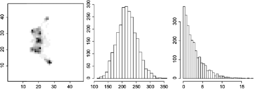
Figure 1: Analysis of real SPECT data: posterior mean reconstruction as a grey-scale image, histogram of marginal posterior for a high-spot pixel (row 12, column 28), and the same for a low-spot pixel (row 12, column 31).

Figure 1 shows selected aspects of this analysis; see caption for details. Our tentative conclusion is that the marginal posterior distributions for individual pixels $\theta_{j}$ do appear to be approximately Gaussian in high-spots and approximately exponential in low-spots, consistent with the theoretical limits presented in Theorem 1.

A second experiment was focussed on a more precise and quantitative assessment of the approximation to the posterior derived in the previous section. The setup is the same as in the first experiment, except at half the resolution, so that reconstruction was on a $24\times 24$ grid of 1.28 cm pixels. The corresponding $A$ matrix is now better-conditioned, and $p$ is only 576, so that manipulation of the matrices is entirely tractable. Synthetic data was generated using this $A$ and a “ground truth” obtained from an approximate MAP reconstruction from the same real data set as used above, yielding photon counts between 0 and 243, totalling 138,310. 50,000 sweeps of the MCMC sampler were used, with prior settings $\gamma=200$, $\zeta=8$.

Figure 2: Agreement between (left panel) the elements of $\hat{a}$ and the reciprocals of the MCMC-computed posterior means of $\theta$, for pixels in $\widehat{S}_{1}$, and also that between (right panel) the diagonal elements of $\widehat{\Omega}{}^{-1}$ and the posterior variances of $\theta$ for pixels in $\widehat{S}_{0}$.

Figure 2 displays the agreement between the elements of $\hat{a}$ and the reciprocals of the MCMC-computed posterior means of $\theta$, for pixels in $\widehat{S}_{1}$, and also that between the diagonal elements of $\widehat{\Omega}{}^{-1}$ and the posterior variances of $\theta$ for pixels in $\widehat{S}_{0}$.

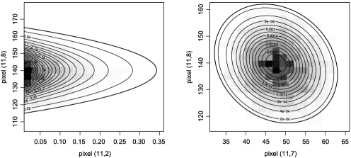
Figure 3: Two bivariate marginals of the posterior, as computed by MCMC (grey-scale image), and the corresponding approximations (contours). In the left panel, one pixel is in $\widehat{S}_{1}$ and one in $\widehat{S}_{0}$, so the approximation is Gaussian/exponential; in the right panel both pixels are from $\widehat{S}_{0}$, so we have a bivariate Gaussian. The outermost contour represents the 95% HPD credible region based on the approximation.

Figure 3 displays two bivariate posterior marginals, computed by MCMC, and the corresponding approximations. In the left panel, one component is in $\widehat{S}_{1}$ and one in $\widehat{S}_{0}$, so the approximation is Gaussian/exponential; on the right both components are from $\widehat{S}_{0}$, so we have a bivariate Gaussian.

We conclude that for this realistic/modest-scale SPECT reconstruction problem, the small-variance asymptotics of this paper provide a good approximation to the posterior, even for $\sigma^{2}=1$.

7 Discussion

When the posterior distribution concentrates on the boundary, we have shown that the classic Bernstein–von Mises theorem does not hold for all components. There are two different types of non-Gaussian component: one, with the same parametric rate of convergence, is a truncated Gaussian or a polynomially tilted modification of this if the prior density is not bounded away from zero and infinity on the boundary, and the second is a Gamma, with a faster rate of convergence. An interesting property of the components of the second type is that they are not subject to a lower bound on efficiency, unlike the “regular” and the first-type boundary components. Under some models with this property, at least part of the data is observed exactly, so perhaps it should not be an unexpected phenomenon; see examples of Poisson and Binomial likelihoods in Section 5. This property is quite remarkable: in principle, it allows the recovery of the unknown parameter on the boundary with an arbitrarily small precision (particularly in the case there is no approximation error), by choosing an appropriate prior distribution, without losing asymptotic efficiency if the parameter is not on the boundary. This property is related to convergence in finitely-many steps of the projected gradient method for a sharp minimum for a noise-free function [Polyak (1983), Theorem 1, page 182; thanks to Alexandre Tsybakov for bringing this to our attention].

A related but different problem involves a nonregular model where the density of the observations has one or more jumps at a point that depends on the unknown parameter, for example, $Y_{i}\sim U[0,\theta]$, $i=1,\ldots,n$, independently. This type of problem has been extensively studied from both frequentist and Bayesian perspectives [Ibragimov and Has’minskiĭ (1981), Ghosh, Ghosal and Samanta (1994), Ghosal and Samanta (1995), Ghosal, Ghosh and Samanta (1995), Chernozhukov and Hong (2004), Hirano and Porter (2003)]. In the problem treated in this paper, the rate of convergence of the posterior distribution of the unknown nonregular parameter as a function of $n$ is the same as in this case where the unknown parameter controls the positions of jumps, faster than the standard parametric rate. However, there is a crucial difference: in the former case, the posterior distribution has a data-dependent random shift, whereas in the latter case there is no such shift.

The nonasymptotic version of the main result shows that other parameters of the model can also affect convergence in practice, such as the smallest eigenvalues of the precision matrices in the $\mathcal{PTN}$ part of the limit and the smallest parameter of the scale of the Gamma distributions.

It is easy to verify that Theorem 1 derived here applies also to misspecified models, with $\mathbb{P}_{\theta^{\star},\sigma}$ being replaced by the true distribution of $\mathbf{Y}$ and $\theta^{\star}$ defined as the unique maximum of $\ell^{\star}(\theta)$ as in Assumption M. This will be discussed elsewhere.

An interesting direction for future work is to study both the behaviour of the posterior distribution, and the question of optimal prior specification, in a framework where the spatial resolution is infinitely refined, placing smoothness class constraints on $\theta^{\star}$.

Appendix: Proofs

.1 Proof of the main result

We start with a lemma.

Lemma 4

Consider the function $\ell_{Y}(\theta)$ defined in Section 3.1 and assume that Assumptions M, B and S hold. Then, on the event $\mathcal{A}_{0}\cap\mathcal{A}_{1}$ defined by (1) with some $\delta_{*0},\delta_{*1}>0$, for $\theta\in\Theta^{\star}(\delta)$,

$$\ell_{Y}(\theta)-\ell_{Y}\bigl{(}\theta^{\star}\bigr{)}$$

$$\qquad\geq\bigl{(}\theta_{S_{0}}-\theta^{\star}_{S_{0}}\bigr{)}^{T}\nabla_{S_{0}}\ell_{Y}\bigl{(}\theta^{\star}\bigr{)}-\bigl{(}\theta_{S_{0}}-\theta^{\star}_{S_{0}}\bigr{)}^{T}\widetilde{\Omega}_{00}\bigl{(}\theta_{S_{0}}-\theta^{\star}_{S_{0}}\bigr{)}/2-\tilde{a}^{T}\theta_{S_{1}},$$

$$\ell_{Y}(\theta)-\ell_{Y}\bigl{(}\theta^{\star}\bigr{)}$$

$$\qquad\leq\bigl{(}\theta_{S_{0}}-\theta^{\star}_{S_{0}}\bigr{)}^{T}\nabla_{S_{0}}\ell_{Y}\bigl{(}\theta^{\star}\bigr{)}-\bigl{(}\theta_{S_{0}}-\theta^{\star}_{S_{0}}\bigr{)}^{T}\overline{\Omega}_{00}\bigl{(}\theta_{S_{0}}-\theta^{\star}_{S_{0}}\bigr{)}/2-\bar{a}^{T}\theta_{S_{1}},$$

where

$$\widetilde{\Omega}_{00} = \Omega_{00}+\delta_{*0}I_{p_{0}},\qquad\overline{\Omega}_{00}=\Omega_{00}-\delta_{*0}I_{p_{0}},$$

$$\tilde{a} = a_{1}+\delta_{*1}\mathbf{1}_{p_{1}},\qquad\bar{a}=a_{1}-\delta_{*1}\mathbf{1}_{p_{1}}.$$

Here $\mathbf{1}_{p_{1}}=(1,\ldots,1)^{T}$—a vector of length $p_{1}$, and $I_{p_{0}}$ is $p_{0}\times p_{0}$ identity matrix.

Applying the Taylor expansion of $\ell_{Y}(\theta)$ as a function of $\theta_{S_{1}}$ at point $\theta^{\star}_{S_{1}}$, and then expanding $\ell_{Y}(\tilde{\theta})$ where $\tilde{\theta}_{S_{0}}=\theta_{S_{0}}$ and $\tilde{\theta}_{S_{1}}=\theta^{\star}_{S_{1}}$, as a function of $\theta_{S_{0}}$ at point $\theta^{\star}_{S_{0}}$, for some $\theta_{c0},\theta_{c1}\in\Theta^{\star}(\delta)$, we have

$$\ell_{Y}(\theta)-\ell_{Y}\bigl{(}\theta^{\star}\bigr{)} = \bigl{(}\theta_{S_{1}}-\theta^{\star}_{S_{1}}\bigr{)}^{T}\nabla_{S_{1}}\ell_{Y}(\theta_{c1})+\bigl{(}\theta_{S_{0}}-\theta^{\star}_{S_{0}}\bigr{)}^{T}\nabla_{S_{0}}\ell_{Y}(\theta)$$

$${}+\bigl{(}\theta_{S_{0}}-\theta^{\star}_{S_{0}}\bigr{)}^{T}\nabla_{S_{0},S_{0}}\ell_{Y}(\theta_{c0})\bigl{(}\theta_{S_{0}}-\theta^{\star}_{S_{0}}\bigr{)}/2.$$

Applying the bounds defining events $\mathcal{A}_{0}$ and $\mathcal{A}_{1}$ to $\nabla_{S_{1}}\ell_{Y}(\theta_{c1})$ and$\nabla_{S_{0},S_{0}}\ell_{Y}(\theta_{c0})$, and using that $\theta_{S_{1}}-\theta^{\star}_{S_{1}}=\theta_{S_{1}}$ is a vector with nonnegative components, we have

$$\ell_{Y}(\theta)-\ell_{Y}\bigl{(}\theta^{\star}\bigr{)} \leq \bigl{(}\theta_{S_{1}}-\theta^{\star}_{S_{1}}\bigr{)}^{T}[-a_{1}+\delta_{*1}1_{|{S_{1}}|}]+\bigl{(}\theta_{S_{0}}-\theta^{\star}_{S_{0}}\bigr{)}^{T}\nabla_{S_{0}}\ell_{Y}(\theta)$$

$${}+\bigl{(}\theta_{S_{0}}-\theta^{\star}_{S_{0}}\bigr{)}^{T}[-\Omega_{00}+\delta_{*0}I_{|S_{0}|}]\bigl{(}\theta_{S_{0}}-\theta^{\star}_{S_{0}}\bigr{)}/2,$$

and hence the first statement of the lemma. Applying the inequalities on the events $\mathcal{A}_{k}$ as lower bounds, we obtain the second statement of the lemma.

Proof of Theorem 1 Denote $v=(v_{0}^{T},v_{1}^{T})^{T}=D^{-1}U(\theta-\theta^{\star})$ where $v_{0}=(\theta_{S_{0}}-\theta^{\star}_{S_{0}})/\sigma$ and $v_{1}=(\theta_{{S_{1}}}-\theta^{\star}_{{S_{1}}})/\sigma^{2}$; the Jacobian of this change of variables is $\sigma^{p_{0}+2p_{1}}$. The image of $\Theta^{\star}(\delta)$ under this transform is

$$B_{R}=B_{2}(0,R_{0})\times[0,R_{1})^{p_{1}}\cap D_{\sigma}^{-1}U\bigl{(}\Theta-\theta^{\star}\bigr{)},$$

with $R_{0}=\delta_{0}/\sigma$ and $R_{1}=\delta_{1}/\sigma^{2}$. Under Assumptions B and S, the conditions of Lemma 2 hold, which implies that if $\|\theta^{\star}_{S_{0}}\|\geq\delta_{0}$ and $\delta_{k}\leq c_{k}$, $B_{R}=[B_{2,p_{0}}(0,R_{0})\cap\mathcal{V}_{0}]\times[0,R_{1}]^{p_{1}}$ where $\mathcal{V}_{0}=\mathbb{R}^{p_{0}-p^{\star}_{0}}\times\mathbb{R}_{+}^{p^{\star}_{0}}$, and the set $B_{R}$ becomes $\mathcal{V}^{\star}=\mathcal{V}_{0}\times\mathbb{R}_{+}^{p_{1}}$ as $\sigma\to 0$.

The triangle inequality for the total variation norm gives

$$\bigl{\|}\mathbb{P}_{{\mathcal{S}}(\theta-\theta^{\star})|Y}-\mu^{\star}\bigr{\|}_{\mathrm{TV}}$$

$$\qquad\leq\bigl{\|}\mathbb{P}_{{\mathcal{S}}(\theta-\theta^{\star})|Y}\mathbf{1}_{B_{R}}-\mu^{\star}\mathbf{1}_{B_{R}}\bigr{\|}_{\mathrm{TV}}$$ (14)

$$\quad\qquad{}+\bigl{\|}\mu^{\star}\mathbf{1}_{B_{R}}-\mu^{\star}\bigr{\|}_{\mathrm{TV}}+\bigl{\|}\mathbb{P}_{{\mathcal{S}}(\theta-\theta^{\star})|Y}\mathbf{1}_{B_{R}}-\mathbb{P}_{{\mathcal{S}}(\theta-\theta^{\star})|Y}\bigr{\|}_{\mathrm{TV}},$$

where the balls $B_{R}$ are defined above. Here $\mu\mathbf{1}_{B_{R}}$ is a probability measure $\mu$ truncated to $B_{R}$ and normalised to be a probability measure. If the measure $\mu_{1}$ is absolutely continuous with respect to measure $\mu_{2}$, with density $f$, the total variation norm can be written as

$$\|\mu_{1}-\mu_{2}\|_{\mathrm{TV}}=2\int_{\Theta}(f-1)_{+}\,d\mu_{2},$$

where $(x)_{+}=\max(x,0)$ [van der Vaart (1998)]. This can be used in each of the summands in the upper bound (.1).

In this proof we will use $\alpha=(\alpha_{0},\alpha_{1})$, for simplicity of notation.

Define the measure $\mu(dv;a_{1},\alpha,b,\Sigma)$ for $v=(v_{0}^{T},v_{1}^{T})^{T}$, $v_{0}\in\mathbb{R}^{p_{0}-p_{0}^{\star}}\times[0,\infty)^{p_{0}^{\star}}$ and $v_{1}\in[0,\infty)^{p_{1}}$, by

$$\frac{\mu(dv;a_{1},\alpha,b,\Sigma)}{dv}=\prod_{j\in T_{0}^{\star}\cup T_{1}}v_{j}^{\alpha_{j}-1}e^{-a_{1}^{T}v_{1}-v_{0}^{T}\Sigma v_{0}/2+v_{0}^{T}b},$$ (15)

where $T_{0}^{\star}=\{p_{0}-p^{\star}_{0}+1,\ldots,p_{0}\}$, $T_{1}=\{p_{0}+1,\ldots,p\}$, $a_{1}\in(0,\infty)^{p_{1}}$, $b\in\mathbb{R}^{p_{0}}$, $\alpha=(\alpha_{j})_{j\in T_{0}^{\star}\cup T_{1}}\in(0,\infty)^{p^{\star}_{0}+p_{1}}$, and $\Sigma$ is a $p_{0}\times p_{0}$ positive definite matrix.

We start with the first term in (.1). By Lemma 4, on the event $\mathcal{A}_{0}\cap\mathcal{A}_{1}$ defined by (1), for any measurable $\mathcal{B}\subseteq\Theta^{\star}(\delta)$, with $\mathcal{B}_{v}=D_{\sigma}^{-1}U(\mathcal{B}-\theta^{\star})\subseteq B_{R}$, we have

$$\int_{\mathcal{B}}\exp\bigl{\{}\bigl{[}\ell_{Y}(\theta)-\ell_{Y}\bigl{(}\theta^{\star}\bigr{)}\bigr{]}/\sigma^{2}\bigr{\}}\pi(d\theta)$$

$$\qquad\geq J_{\sigma}C_{\pi}(1-\Delta_{\pi})$$

$$\quad\qquad{}\times\int_{\mathcal{B}_{v}}\prod_{j\in T_{0}^{\star}\cup T_{1}}v_{j}^{\alpha_{j}-1}\exp\bigl{\{}v_{0}^{T}\nabla_{S_{0}}\ell_{Y}\bigl{(}\theta^{\star}\bigr{)}/\sigma-\bigl{\|}\widetilde{\Omega}_{00}^{1/2}v_{0}\bigr{\|}^{2}/2-\tilde{a}^{T}v_{1}\bigr{\}}\,dv$$

$$\qquad=J_{\sigma}C_{\pi}(1-\Delta_{\pi})\mu\bigl{(}\mathcal{B}_{v};\tilde{a},\alpha,\nabla_{S_{0}}\ell_{Y}\bigl{(}\theta^{\star}\bigr{)}/\sigma,\widetilde{\Omega}_{00}\bigr{)},$$

where $J_{\sigma}=\sigma^{p_{0}-p^{\star}_{0}+\sum_{j\in T_{0}^{\star}}\alpha_{0,j}+2\sum_{j=1}^{p_{1}}\alpha_{1,j}}$, and the measure $\mu(dv;a_{1},\alpha,b,\Sigma)$ is defined by (15). Similarly, using Lemma 4, we obtain an upper bound on the event $\mathcal{A}_{0}\cap\mathcal{A}_{1}$,

$$\int_{\mathcal{B}}\exp\bigl{\{}\bigl{[}\ell_{Y}(\theta)-\ell_{Y}\bigl{(}\theta^{\star}\bigr{)}\bigr{]}/\sigma^{2}\bigr{\}}\pi(d\theta)$$

$$\qquad\leq J_{\sigma}C_{\pi}(1+\Delta_{\pi})$$

$$\quad\qquad{}\times\int_{\mathcal{B}_{v}}\prod_{j\in T_{0}^{\star}\cup T_{1}}v_{j}^{\alpha_{j}-1}\exp\bigl{\{}v_{0}^{T}\nabla_{S_{0}}\ell_{Y}\bigl{(}\theta^{\star}\bigr{)}/\sigma-\bigl{\|}\overline{\Omega}_{00}^{1/2}v_{0}\bigr{\|}^{2}/2-\bar{a}^{T}v_{1}\bigr{\}}\,dv$$

$$\qquad=J_{\sigma}C_{\pi}(1+\Delta_{\pi})\mu\bigl{(}\mathcal{B}_{v};\bar{a},\alpha,\nabla_{S_{0}}\ell_{Y}\bigl{(}\theta^{\star}\bigr{)}/\sigma,\overline{\Omega}_{00}\bigr{)}.$$

To simplify the notation, denote $a_{0}=\Omega_{00}^{-1}\nabla_{S_{0}}\ell_{Y}(\theta^{\star})/\sigma$ and

$$\bar{\mu}(dv) = \mu(dv;\bar{a},\alpha,\Omega_{00}a_{0},\overline{\Omega}_{00}),$$

$$\tilde{\mu}(dv) = \mu(dv;\tilde{a},\alpha,\Omega_{00}a_{0},\widetilde{\Omega}_{00}).$$

The measure $\tilde{\mu}$ is finite since $a_{0}=\nabla_{S_{0}}\ell_{Y}(\theta^{\star})/\sigma$ is finite with high probability due to Assumption S(4), and all its other parameters are positive or positive definite. The measure $\bar{\mu}$ is finite if $\delta_{*1}<\min_{j}a_{1,j}$ and $\delta_{*0}<\lambda_{\min}(\Omega_{00})$. These conditions hold if $\delta_{*0},\delta_{*1}$ are small enough which is possible due to Assumption S.

For $\mathcal{B}_{v}=\mathcal{B}_{1}\times B_{\infty}(0,r_{1})$ for some $\mathcal{B}_{1}\subset\mathcal{V}_{0}$ and $r_{1}\in(0,R_{1})$, we have

$$\mu\bigl{(}\mathcal{V}^{\star};a_{1},\alpha,b,\Sigma\bigr{)} = \prod_{i=1}^{p_{1}}\bigl{[}a_{1,i}^{-\alpha_{1,i}}\Gamma(\alpha_{1,i})\bigr{]}\int_{\mathcal{V}_{0}}\prod_{j\in T_{0}^{\star}}v_{0,j}^{\alpha_{0,j}-1}e^{-v_{0}^{T}\Sigma v_{0}/2+v_{0}^{T}b}\,dv_{0},$$

$$\frac{\mu(\mathcal{B}_{v};a_{1},\alpha,b,\Sigma)}{\mu(\mathcal{V}^{\star};a_{1},\alpha,b,\Sigma)} = \mathcal{PTN}_{p_{0}}\bigl{(}\mathcal{B}_{1};\Sigma^{-1}b,\Sigma^{-1},p_{0}^{\star},\alpha_{0}\bigr{)}\prod_{j=1}^{p_{1}}\Gamma\bigl{(}(0,r_{1});\alpha_{1,j},a_{1,j}\bigr{)},$$

where the probability measure $\mathcal{PTN}_{p_{0}}(\cdot;b,\Omega_{00}^{-1},p_{0}^{\star},\alpha_{0})$ is defined by (4.1), and $\Gamma(\cdot;\alpha_{1,j},a_{1,j})$ is the probability measure associated with distribution $\Gamma(\alpha_{1,j},a_{1,j})$.

Hence, the posterior density of ${\mathcal{S}}(\theta-\theta^{\star})$ normalised by the posterior measure of $B_{R}$, is bounded on $\mathcal{A}_{0}\cap\mathcal{A}_{1}$ by

$$\frac{1-\Delta_{\pi}}{1+\Delta_{\pi}}\frac{\tilde{\mu}(dv)}{\bar{\mu}(B_{R})}\leq\frac{dp({\mathcal{S}}(\theta-\theta^{\star})|Y)}{p(B_{R}|Y)}\leq\frac{\bar{\mu}(dv)}{\tilde{\mu}(B_{R})}\frac{1+\Delta_{\pi}}{1-\Delta_{\pi}}.$$

Therefore, the first term in (.1) is bounded on $\mathcal{A}_{0}\cap\mathcal{A}_{1}$ by

$$\bigl{\|}\mathbb{P}_{{\mathcal{S}}(\theta-\theta^{\star})|Y}\mathbf{1}_{B_{R}}-\mu^{\star}\mathbf{1}_{B_{R}}\bigr{\|}_{\mathrm{TV}}$$

$$\qquad\leq 2\int_{B_{R}}\biggl{[}\frac{\mathbb{P}(dv|Y)\mu^{\star}(B_{R})}{\mathbb{P}(B_{R}|Y)\mu^{\star}(dv)}-1\biggr{]}_{+}\frac{\mu^{\star}(dv)}{\mu^{\star}(B_{R})}$$

$$\qquad\leq 2\int_{B_{R}}\biggl{[}\frac{\bar{\mu}(dv)}{\tilde{\mu}(B_{R})}\frac{\mu^{\star}(B_{R})}{\mu^{\star}(dv)}\frac{(1+\Delta_{\pi})}{(1-\Delta_{\pi})}-1\biggr{]}_{+}\frac{\mu^{\star}(dv)}{\mu^{\star}(B_{R})}.$$

Define $\mu_{0}(dv)=\mu(dv;a_{1},\alpha,\Omega_{00}a_{0},\Omega_{00})$. Then

$$\frac{\mu^{\star}(dv)}{\mu^{\star}(B_{R})}=\frac{\mu_{0}(dv)}{\mu_{0}(B_{R})}$$

and

$$\frac{\bar{\mu}(dv)}{\mu_{0}(dv)}=\exp\bigl{\{}\delta_{*1}\mathbf{1}^{T}v_{1}+\delta_{*0}\|v_{0}\|^{2}/2\bigr{\}},$$

which implies

$$\frac{\bar{\mu}(dv)}{\mu_{0}(dv)}\frac{\mu_{0}(B_{R})}{\tilde{\mu}(B_{R})}$$

$$\qquad=\exp\bigl{\{}\delta_{*0}\|v_{0}\|^{2}/2+\delta_{*1}\mathbf{1}^{T}v_{1}\bigr{\}}$$

$$\quad\qquad{}\times\Biggl{(}{\int_{B_{R}}\prod_{i\in T_{0}^{\star}\cup T_{1}}v_{i}^{\alpha_{i}-1}\exp\bigl{\{}-a_{1}^{T}v_{1}\bigr{\}}\exp\bigl{\{}-\bigl{\|}\Omega_{00}^{1/2}v_{0}\bigr{\|}^{2}/2+v_{0}^{T}\Omega_{00}a_{0}\bigr{\}}\,dv}\Biggr{)}$$

$$\hskip 48.0pt\bigg{/}\Biggl{(}\int_{B_{R}}\prod_{i\in T_{0}^{\star}\cup T_{1}}v_{i}^{\alpha_{i}-1}\exp\bigl{\{}-(a_{1}+\delta_{*1}\mathbf{1})^{T}v_{1}-\bigl{\|}\widetilde{\Omega}_{00}^{1/2}v_{0}\bigr{\|}^{2}/2$$

$$\hskip 259.0pt{}+v_{0}^{T}\Omega_{00}a_{0}\bigr{\}}\,dv\Biggr{)}.$$

To show that this expression is greater than 1, it is sufficient to show that for any $\mathcal{B}\subseteq\{v_{0}\dvtx(v_{0}^{T},v_{1}^{T})^{T}\in B_{R}\}$, the following expression is positive:

$$\int_{\mathcal{B}}\prod_{i\in T_{0}^{\star}}w_{i}^{\alpha_{i}-1}e^{w^{T}\Omega_{00}a_{0}-\|\Omega_{00}^{1/2}w\|^{2}/2}\,dw-\int_{\mathcal{B}}\prod_{i\in T_{0}^{\star}}w_{i}^{\alpha_{i}-1}e^{w^{T}\Omega_{00}a_{0}-\|\widetilde{\Omega}_{00}^{1/2}w\|^{2}/2}\,dw$$

$$\qquad=\int_{\mathcal{B}}\prod_{i\in T_{0}^{\star}}w_{i}^{\alpha_{i}-1}e^{-\|\widetilde{\Omega}_{00}^{1/2}w\|^{2}/2+w^{T}\Omega_{00}a_{0}}\bigl{[}\exp\bigl{\{}\delta_{*0}\|w\|^{2}/2\bigr{\}}-1\bigr{]}\,dw>0$$

which is the case. Thus, on $\mathcal{A}_{0}\cap\mathcal{A}_{1}$, $(\bar{\mu}(dv)/\mu_{0}(dv))(\mu_{0}(B_{R})/\tilde{\mu}(B_{R}))\geq 1$ and hence

$$\bigl{\|}\mathbb{P}_{{\mathcal{S}}(\theta-\theta^{\star})|Y}\mathbf{1}_{B_{R}}-\mu^{\star}\mathbf{1}_{B_{R}}\bigr{\|}_{\mathrm{TV}}$$

$$\qquad\leq 2\int_{B_{R}}\biggl{[}\frac{\bar{\mu}(dv)}{\tilde{\mu}(B_{R})}\frac{\mu^{\star}(B_{R})}{\mu^{\star}(dv)}\frac{(1+\Delta_{\pi})}{(1-\Delta_{\pi})}-1\biggr{]}\frac{\mu^{\star}(dv)}{\mu^{\star}(B_{R})}$$

$$\qquad=2\biggl{[}\frac{\bar{\mu}(B_{R})}{\tilde{\mu}(B_{R})}\frac{(1+\Delta_{\pi})}{(1-\Delta_{\pi})}-1\biggr{]}$$

$$\qquad=2\frac{\bar{\mu}(B_{R})-\tilde{\mu}(B_{R})}{\tilde{\mu}(B_{R})}\frac{(1+\Delta_{\pi})}{(1-\Delta_{\pi})}+2\biggl{[}\frac{(1+\Delta_{\pi})}{(1-\Delta_{\pi})}-1\biggr{]}.$$

The difference of measures $\bar{\mu}(B_{R})-\tilde{\mu}(B_{R})$ is bounded by

$$\int_{B_{R}}\prod_{i\in T_{0}^{\star}\cup T_{1}}v_{i}^{\alpha_{i}-1}e^{-v_{0}^{T}\widetilde{\Omega}_{00}v_{0}/2+v_{0}^{T}\Omega_{00}a_{0}-\tilde{a}v_{1}}\bigl{[}e^{\delta_{*0}\|v_{0}\|^{2}/2+\delta_{*1}1_{p_{1}}^{T}v_{1}}-1\bigr{]}\,dv$$

$$\qquad\leq\int_{B_{R}}\prod_{i\in T_{0}^{\star}\cup T_{1}}v_{i}^{\alpha_{i}-1}\bigl{[}\delta_{*0}\|v_{0}\|^{2}/2+\delta_{*1}1_{p_{1}}^{T}v_{1}\bigr{]}e^{-v_{0}^{T}\overline{\Omega}_{00}v_{0}/2+v_{0}^{T}\Omega_{00}a_{0}-\bar{a}v_{1}}\,dv$$

$$\qquad\leq\Biggl{[}\delta_{*0}E_{\Phi}+\delta_{*1}\sum_{j=1}^{p_{1}}(\alpha_{1,j}/\bar{a}_{j})\Biggr{]}\bar{\mu}\bigl{(}\mathcal{V}^{\star}\bigr{)}$$

due to the inequality $e^{x}-1\leq xe^{x}$ for $x>0$, where $E_{\Phi}$ is defined by

$$E_{\Phi}=0.5\int_{\mathcal{V}_{0}}\|w\|^{2}\mathcal{PTN}_{p_{0}}\bigl{(}dw;\overline{\Omega}_{00}^{-1}\Omega_{00}a_{0},\overline{\Omega}_{00}^{-1},p_{0}^{\star},\alpha_{0}\bigr{)},$$ (16)

which is finite. Therefore,

$$\bigl{\|}\mathbb{P}_{{\mathcal{S}}(\theta-\theta^{\star})|Y}\mathbf{1}_{B_{R}}-\mu^{\star}\mathbf{1}_{B_{R}}\bigr{\|}_{\mathrm{TV}}$$

$$\qquad\leq\frac{2\bar{\mu}(\mathcal{V}^{\star})}{\tilde{\mu}(B_{R})}\frac{(1+\Delta_{\pi})}{(1-\Delta_{\pi})}\Biggl{[}\delta_{*0}E_{\Phi}+\delta_{*1}\sum_{j=1}^{p_{1}}\frac{\alpha_{1,j}}{\bar{a}_{j}}\Biggr{]}+\frac{4\Delta_{\pi}}{1-\Delta_{\pi}},$$

which goes to zero since $\delta_{*k}\to 0$ and $\Delta_{\pi}\to 0$ as $\sigma\to 0$. For small $\sigma$ and hence large $R_{0}$ and $R_{1}$, the ratios $\bar{\mu}(\mathcal{V}^{\star})/\tilde{\mu}(\mathcal{V}^{\star})$ and

$$\frac{\tilde{\mu}(B_{R})}{\tilde{\mu}(\mathcal{V}^{\star})}=\mathcal{PTN}_{p_{0}}\bigl{(}B_{2}(0,R_{0});\widetilde{\Omega}_{00}^{-1}\Omega_{00}a_{0},\widetilde{\Omega}_{00}^{-1},p^{\star}_{0},\alpha_{0}\bigr{)}\prod_{j=1}^{p_{1}}\Gamma\bigl{(}(0,R_{1});\alpha_{1,j},\tilde{a}_{j}\bigr{)}$$

are close to 1. Therefore, $\|\mathbb{P}_{{\mathcal{S}}(\theta-\theta^{\star})|Y}\mathbf{1}_{B_{R}}-\mu^{\star}\mathbf{1}_{B_{R}}\|_{\mathrm{TV}}\to 0$ as $\sigma\to 0$.

The second term in (.1) is bounded by $\|\mu^{\star}-\mu^{\star}\mathbf{1}_{B_{R}}\|_{\mathrm{TV}}\leq 2\mu^{\star}(\overline{B_{R}})\to 0$ as $R_{0},R_{1}\to\infty$, since the set $B_{R}$ converges to $\mathcal{V}^{\star}$ by Lemma 2.

The third term in (.1) is bounded by

$$\bigl{\|}\mathbb{P}_{({\mathcal{S}}(\theta-\theta^{\star})|Y)}\mathbf{1}_{B_{R}}-\mathbb{P}_{{\mathcal{S}}(\theta-\theta^{\star})|Y}\bigr{\|}_{\mathrm{TV}}\leq 2\mathbb{P}_{{\mathcal{S}}(\theta-\theta^{\star})|Y}(\overline{B_{R}})\leq\frac{2\Delta_{0}(\delta)}{C_{\pi}(1-\Delta_{\pi})\tilde{\mu}(B_{R})},$$

where $\Delta_{0}(\delta)$ is defined by (6). By Assumption L, with probability $\to 1$, $\Delta_{0}(\delta)\to 0$ as $\sigma\to 0$; also, $\tilde{\mu}(B_{R})\to\mu_{0}(\mathcal{V}^{\star})>0$.

Combining these bounds, we have that on $\mathcal{A}_{0}\cap\mathcal{A}_{1}$,

$$\bigl{\|}\mathbb{P}_{{\mathcal{S}}(\theta-\theta^{\star})|Y}-\mu^{\star}\bigr{\|}_{\mathrm{TV}}$$

$$\qquad\leq 2\mu^{\star}(\overline{B_{R}})+2\bigl{[}C_{\pi}(1-\Delta_{\pi})\tilde{\mu}(B_{R})\bigr{]}^{-1}\Delta_{0}(\delta)$$

$$\quad\qquad{}+2\frac{\bar{\mu}(\mathcal{V}^{\star})}{\tilde{\mu}(B_{R})}\frac{(1+\Delta_{\pi})}{(1-\Delta_{\pi})}\Biggl{[}\delta_{*0}E_{\Phi}+\delta_{*1}\sum_{j=1}^{p_{1}}(\alpha_{1,j}/\bar{a}_{j})\Biggr{]}+\frac{4\Delta_{\pi}}{(1-\Delta_{\pi})}\to 0$$

and $\mathbb{P}_{\theta^{\star},\sigma}(\mathcal{A}_{0}\cap\mathcal{A}_{1})\to 1$ as $\sigma\to 0$ due to Assumption S, which gives the statement of the theorem.

Proof of Proposition 1 In the proof of Theorem 1, we derived the following upper bound on event $\mathcal{A}$:

$$\bigl{\|}\mathbb{P}_{{\mathcal{S}}(\theta-\theta^{\star})|Y}-\mu^{\star}\bigr{\|}_{\mathrm{TV}}\leq 2\mu^{\star}(\overline{B_{R}})+C_{\Delta}\Delta_{0}(\delta)+2C_{0}\delta_{*0}+2C_{1}\delta_{*1}+C_{2}\Delta_{\pi},$$

where $C_{\Delta}=2[C_{\pi}(1-\Delta_{\pi})\tilde{\mu}(B_{R})]^{-1}$, $C_{2}=4/(1-\Delta_{\pi})$, $C_{0}=C_{A}E_{\Phi}$ with $E_{\Phi}$ defined by (16), $C_{1}=C_{A}\sum_{j=1}^{p_{1}}\alpha_{1,j}/(a_{1,j}-\delta_{*1})$ and with $B_{R,0}=\break B_{2,p_{0}}(0,R_{0})\cap\mathcal{V}_{0}$,

$$C_{A}=\frac{\bar{\mu}(\mathcal{V}^{\star})}{\tilde{\mu}(B_{R})}\frac{(1+\Delta_{\pi})}{(1-\Delta_{\pi})}=\frac{\bar{\mu}_{p_{0}}(\mathcal{V}_{0})}{\tilde{\mu}_{p_{0}}(B_{R,0})}\prod_{j=1}^{p_{1}}\biggl{[}\frac{a_{1,j}+\delta_{*1}}{a_{1,j}-\delta_{*1}}\biggr{]}^{\alpha_{1,j}}\frac{(1+\Delta_{\pi})}{(1-\Delta_{\pi})},$$

where $\mu_{p_{0}}(\mathcal{B}_{0})=\int_{\mathcal{B}_{0}\times[0,\infty)^{p_{1}}}\mu(dv)$ for a measure $\mu$, $\mathcal{B}_{0}\subset\mathcal{V}_{0}$. If $S_{0}^{\star}=\varnothing$,

$$E_{\Phi} = \bigl{\|}\overline{\Omega}_{00}^{-1}\Omega_{00}a_{0}\bigr{\|}^{2}/2+\operatorname{trace}\bigl{(}\overline{\Omega}_{00}^{-1}\bigr{)}/2,$$

$$\frac{\bar{\mu}_{p_{0}}(\mathcal{V}_{0})}{\tilde{\mu}_{p_{0}}(B_{R,0})} = \frac{e^{\delta_{*0}a_{0}^{T}\Omega_{00}\overline{\Omega}_{00}^{-1}\widetilde{\Omega}_{00}^{-1}\Omega_{00}a_{0}}[\det(\overline{\Omega}_{00}^{-1}\widetilde{\Omega}_{00})]^{1/2}}{\mathcal{TN}(B_{R,0};\widetilde{\Omega}_{00}^{-1}\Omega_{00}a_{0},\widetilde{\Omega}_{00}^{-1})}.$$

We bound the term $\mu^{\star}(\overline{B_{R}})$ by

$$\mu^{\star}(\overline{B_{R}}) = 1-\mu^{\star}_{p_{0}}(B_{R,0})\prod_{j=1}^{p_{1}}\Gamma\biggl{(}\biggl{(}0,\frac{\delta_{1}}{\sigma^{2}}\biggr{)};\alpha_{1,j},a_{1,j}\biggr{)}$$

$$\leq \mu^{\star}_{p_{0}}(\overline{B_{R,0}})+1-\prod_{j=1}^{p_{1}}\Gamma\biggl{(}\biggl{(}0,\frac{\delta_{1}}{\sigma^{2}}\biggr{)};\alpha_{1,j},a_{1,j}\biggr{)}$$

using the inequality $1-xy\leq 1-x+1-y$ for $x,y\in(0,1)$. We can also use

$$1-\prod_{j=1}^{p_{1}}\Gamma\biggl{(}\biggl{(}0,\frac{\delta_{1}}{\sigma^{2}}\biggr{)};\alpha_{1,j},a_{1,j}\biggr{)} \leq p_{1}\Bigl{[}1-\min_{j}\Gamma\bigl{(}\bigl{(}0,\delta_{1}/\sigma^{2}\bigr{)};\alpha_{1,j},a_{1,j}\bigr{)}\Bigr{]}$$

$$= p_{1}\max_{j}\Gamma\bigl{(}\bigl{(}\delta_{1}/\sigma^{2},\infty\bigr{)};\alpha_{1,j},a_{1,j}\bigr{)},$$

and, changing to polar coordinates and denoting $p_{\alpha 0}=p_{0}+\sum_{j\in T_{0}^{\star}}(\alpha_{0,j}-1)$ and $W=\{w\in\mathbb{R}^{p_{0}}\dvtx\|w\|_{2}^{2}=1,w_{j}>0$ for $j\in T_{0}^{\star}\}$, we have

$$\mu^{\star}_{p_{0}}(\overline{B_{R,0}}) \leq \mu_{0}\bigl{(}\mathcal{V}^{\star}\bigr{)}\int_{R_{0}}^{\infty}r^{p_{\alpha 0}-1}e^{-\lambda_{\min}(\Omega_{00})(r-\|a_{0}\|)^{2}/2}\,dr\int_{W}\prod_{j\in T_{0}^{\star}}w_{j}^{\alpha_{0,j}-1}\,dw$$

$$\leq C_{\alpha 0}\Gamma\bigl{(}\bigl{(}\bigl{(}\delta_{0}/\sigma-\|a_{0}\|\bigr{)}^{2}/2,\infty\bigr{)};p_{\alpha 0}/2,\lambda_{\min}(\Omega_{00})\bigr{)}$$

under the assumption that $R_{0}=\delta_{0}/\sigma>\|a_{0}(\omega)\|$ where

$$C_{\alpha 0}=\mu_{0}\bigl{(}\mathcal{V}^{\star}\bigr{)}2^{-p_{0}^{\star}+1.5p_{\alpha 0}}\bigl{[}\lambda_{\min}(\Omega_{00})\bigr{]}^{p_{\alpha 0}/2}\pi^{(p_{0}-p^{\star}_{0})/2}\prod_{i\in T_{0}^{\star}}\Gamma(\alpha_{0,i}/2).$$

Collecting conditions on $\delta_{k}$ used in the proof of Theorem 1, we have conditions (1). Thus, we have the required inequality on the event $\mathcal{A}$.

.2 Auxiliary results

Proof of Lemma 2 Due to Assumption B and the fact that $\theta^{\star}_{S^{\star}_{0}\cup S_{1}}=0$, the set $D^{-1}U(\Theta^{\star}(\delta)-\theta^{\star})$ contains

$$B_{2,p_{0}}\biggl{(}0,\frac{\delta_{0}}{\sigma}\biggr{)}\times B_{\infty,p_{1}}\biggl{(}0,\frac{\delta_{1}}{\sigma^{2}}\biggr{)}\cap\biggl{(}-\frac{c_{0}}{\sigma},\frac{c_{0}}{\sigma}\biggr{)}^{p_{0}-p_{0}^{\star}}\times\biggl{[}0,\frac{c_{0}}{\sigma}\biggr{)}^{p_{0}^{\star}}\times\biggl{[}0,\frac{c_{1}}{\sigma^{2}}\biggr{)}^{p_{1}}$$

$$\qquad=\bigl{\{}v\dvtx v\in B_{2,p_{0}}(0,\delta_{0}/\sigma)\mbox{ and }v_{T_{0}^{\star}}\geq 0\bigr{\}}\times\bigl{[}0,\delta_{1}/\sigma^{2}\bigr{)}^{p_{1}},$$

where $T_{0}^{\star}=\{p_{0}-p_{0}^{\star}+1,\ldots,p_{0}\}$. These sets monotonically increase to $\mathcal{V}^{\star}=\mathbb{R}^{p_{0}-p^{\star}_{0}}\times\mathbb{R}^{p^{\star}_{0}+p_{1}}_{+}$ as $\sigma\to 0$ due to the assumption $\delta_{0}/\sigma\to\infty$ and $\delta_{1}/\sigma^{2}\to\infty$; this implies the statement of the lemma.

Proof of Lemma 3 Under the assumptions of the lemma, for small enough $\sigma$, with $\tilde{\delta}_{0}=\delta_{0}/\sqrt{p_{0}}$, we have that

$$\frac{1}{C_{\pi 0}(\delta)}\int_{\Theta\setminus\Theta^{\star}(\delta)}e^{(\ell_{y}(\theta)-\ell_{y}(\theta^{\star}))/\sigma^{2}}\pi(d\theta)$$

$$\qquad\leq\sum_{j\in S_{0}}\int_{\tilde{\delta}_{0}}^{\infty}e^{-C_{\delta 0}v_{j}/\sigma^{2}}\,dv_{j}$$

$$\quad\qquad{}+\sum_{j\in S_{0}\setminus S_{0}^{\star}}\int_{0}^{\theta^{\star}_{j}-\tilde{\delta}_{0}}\theta_{j}^{\bolds\alpha_{j}-1}e^{-C_{\delta 0}|\theta_{j}-\theta^{\star}_{j}|/\sigma^{2}}\,d\theta_{j}$$

$$\quad\qquad{}+\sum_{j\in S_{1}}\int_{\delta_{1}}^{\infty}e^{-C_{\delta 1}v_{j}/\sigma^{2}}\,dv_{j}$$

$$\qquad\leq\sum_{j\in S_{0}\setminus S_{0}^{\star}}\sigma^{\bolds\alpha_{j}}e^{-C_{\delta 0}(\theta^{\star}_{j}-\sigma)/\sigma^{2}}+\frac{p_{0}\sigma^{2}}{C_{\delta 0}}e^{-C_{\delta}\delta_{0}/[\sqrt{p_{0}}\sigma^{2}]}+\frac{p_{1}\sigma^{2}}{C_{\delta 1}}e^{-C_{\delta 1}\delta_{1}/\sigma^{2}}$$

$$\quad\qquad{}+\sum_{j\in S_{0}\setminus S_{0}^{\star}}\bigl{[}\sigma^{\bolds\alpha_{j}-1}I(\bolds\alpha_{j}<1)+{\theta^{\star}_{j}}^{\bolds\alpha_{j}-1}I(\bolds\alpha_{j}\geq 1)\bigr{]}\frac{\sigma^{2}}{C_{\delta 0}}e^{-C_{\delta 0}\tilde{\delta}_{0}/\sigma^{2}}$$

$$\qquad\leq C\bigl{[}\sigma^{\min_{j}(\bolds\alpha_{j})}+\sigma\bigr{]}e^{-C_{\delta 0}\delta_{0}/[\sqrt{p_{0}}\sigma^{2}]}+p_{1}e^{-C_{\delta 1}\delta_{1}/\sigma^{2}}\sigma^{2}/C_{\delta 1}$$

for a constant $C$. This implies that, with $J_{\sigma}=\sigma^{-\sum_{j\in S_{0}}\bolds\alpha_{j}-2\sum_{j\in S_{1}}\bolds\alpha_{j}}$,

$$\Delta_{0}(\delta)\leq C_{\pi 0}(\delta)J_{\sigma}\biggl{[}C\bigl{[}\sigma^{\min_{j}(\bolds\alpha_{j})}+\sigma\bigr{]}e^{-C_{\delta 0}\delta_{0}/[\sqrt{p_{0}}\sigma^{2}]}+\frac{p_{1}\sigma^{2}}{C_{\delta 1}}e^{-C_{\delta 1}\delta_{1}/\sigma^{2}}\biggr{]}\to 0$$

as $\sigma\to 0$ under the assumptions of the lemma.

References

• Barron, Schervish and Wasserman (1999) {barticle}[mr] \bauthor\bsnmBarron, \bfnmAndrew\binitsA., \bauthor\bsnmSchervish, \bfnmMark J.\binitsM. J. and \bauthor\bsnmWasserman, \bfnmLarry\binitsL. (\byear1999). \btitleThe consistency of posterior distributions in nonparametric problems. \bjournalAnn. Statist. \bvolume27 \bpages536–561. \biddoi=10.1214/aos/1018031206, issn=0090-5364, mr=1714718 \bptokimsref\endbibitem
• Bertsekas (2003) {bbook}[author] \bauthor\bsnmBertsekas, \bfnmD. P.\binitsD. P. (\byear2003). \btitleConvex Analysis and Optimization. \bpublisherAthena Scientific and Tsinghua Univ. Press, \blocationBelmont, MA. \bptokimsref\endbibitem
• Besag (1986) {barticle}[mr] \bauthor\bsnmBesag, \bfnmJulian\binitsJ. (\byear1986). \btitleOn the statistical analysis of dirty pictures. \bjournalJ. Roy. Statist. Soc. Ser. B \bvolume48 \bpages259–302. \bidissn=0035-9246, mr=0876840 \bptnotecheck related \bptokimsref\endbibitem
• Bochkina (2013) {barticle}[mr] \bauthor\bsnmBochkina, \bfnmNatalia\binitsN. (\byear2013). \btitleConsistency of the posterior distribution in generalized linear inverse problems. \bjournalInverse Problems \bvolume29 \bpages095010, 43. \biddoi=10.1088/0266-5611/29/9/095010, issn=0266-5611, mr=3094485 \bptokimsref\endbibitem
• Chernozhukov and Hong (2004) {barticle}[mr] \bauthor\bsnmChernozhukov, \bfnmVictor\binitsV. and \bauthor\bsnmHong, \bfnmHan\binitsH. (\byear2004). \btitleLikelihood estimation and inference in a class of nonregular econometric models. \bjournalEconometrica \bvolume72 \bpages1445–1480. \biddoi=10.1111/j.1468-0262.2004.00540.x, issn=0012-9682, mr=2077489 \bptokimsref\endbibitem
• Douc et al. (2011) {barticle}[mr] \bauthor\bsnmDouc, \bfnmRandal\binitsR., \bauthor\bsnmMoulines, \bfnmEric\binitsE., \bauthor\bsnmOlsson, \bfnmJimmy\binitsJ. and \bauthor\bparticlevan \bsnmHandel, \bfnmRamon\binitsR. (\byear2011). \btitleConsistency of the maximum likelihood estimator for general hidden Markov models. \bjournalAnn. Statist. \bvolume39 \bpages474–513. \biddoi=10.1214/10-AOS834, issn=0090-5364, mr=2797854 \bptokimsref\endbibitem
• Dudley and Haughton (2002) {barticle}[mr] \bauthor\bsnmDudley, \bfnmR. M.\binitsR. M. and \bauthor\bsnmHaughton, \bfnmD.\binitsD. (\byear2002). \btitleAsymptotic normality with small relative errors of posterior probabilities of half-spaces. \bjournalAnn. Statist. \bvolume30 \bpages1311–1344. \biddoi=10.1214/aos/1035844978, issn=0090-5364, mr=1936321 \bptokimsref\endbibitem
• Erkanli (1994) {barticle}[mr] \bauthor\bsnmErkanli, \bfnmAlaattin\binitsA. (\byear1994). \btitleLaplace approximations for posterior expectations when the mode occurs at the boundary of the parameter space. \bjournalJ. Amer. Statist. Assoc. \bvolume89 \bpages250–258. \bidissn=0162-1459, mr=1266297 \bptokimsref\endbibitem
• Geman and Geman (1984) {barticle}[pbm] \bauthor\bsnmGeman, \bfnmS.\binitsS. and \bauthor\bsnmGeman, \bfnmD.\binitsD. (\byear1984). \btitleStochastic relaxation, gibbs distributions, and the Bayesian restoration of images. \bjournalIEEE Trans. Pattern Anal. Mach. Intell. \bvolume6 \bpages721–741. \bidissn=0162-8828, pmid=22499653 \bptokimsref\endbibitem
• Ghosal, Ghosh and Samanta (1995) {barticle}[mr] \bauthor\bsnmGhosal, \bfnmSubhashis\binitsS., \bauthor\bsnmGhosh, \bfnmJayanta K.\binitsJ. K. and \bauthor\bsnmSamanta, \bfnmTapas\binitsT. (\byear1995). \btitleOn convergence of posterior distributions. \bjournalAnn. Statist. \bvolume23 \bpages2145–2152. \biddoi=10.1214/aos/1034713651, issn=0090-5364, mr=1389869 \bptokimsref\endbibitem
• Ghosal and Samanta (1995) {barticle}[mr] \bauthor\bsnmGhosal, \bfnmSubhashis\binitsS. and \bauthor\bsnmSamanta, \bfnmTapas\binitsT. (\byear1995). \btitleAsymptotic behaviour of Bayes estimates and posterior distributions in multiparameter nonregular cases. \bjournalMath. Methods Statist. \bvolume4 \bpages361–388. \bidissn=1066-5307, mr=1372011 \bptokimsref\endbibitem
• Ghosh, Ghosal and Samanta (1994) {bincollection}[mr] \bauthor\bsnmGhosh, \bfnmJayanta K.\binitsJ. K., \bauthor\bsnmGhosal, \bfnmSubhashis\binitsS. and \bauthor\bsnmSamanta, \bfnmTapas\binitsT. (\byear1994). \btitleStability and convergence of the posterior in non-regular problems. In \bbooktitleStatistical Decision Theory and Related Topics, V (West Lafayette, IN, 1992) (\beditor\bfnmS. S.\binitsS. S. \bsnmGupta and \beditor\bfnmJ. O.\binitsJ. O. \bsnmBerger, eds.) \bpages183–199. \bpublisherSpringer, \blocationNew York. \bidmr=1286304 \bptokimsref\endbibitem
• Green (1990) {barticle}[author] \bauthor\bsnmGreen, \bfnmPeter J.\binitsP. J. (\byear1990). \btitleBayesian reconstructions from emission tomography data using a modified EM algorithm. \bjournalIEEE Trans. Med. Imag. \bvolume9 \bpages84–93. \bptokimsref\endbibitem
• Hirano and Porter (2003) {barticle}[mr] \bauthor\bsnmHirano, \bfnmKeisuke\binitsK. and \bauthor\bsnmPorter, \bfnmJack R.\binitsJ. R. (\byear2003). \btitleAsymptotic efficiency in parametric structural models with parameter-dependent support. \bjournalEconometrica \bvolume71 \bpages1307–1338. \biddoi=10.1111/1468-0262.00451, issn=0012-9682, mr=2000249 \bptokimsref\endbibitem
• Ibragimov and Has’minskiĭ (1981) {bbook}[mr] \bauthor\bsnmIbragimov, \bfnmI. A.\binitsI. A. and \bauthor\bsnmHas’minskiĭ, \bfnmR. Z.\binitsR. Z. (\byear1981). \btitleStatistical Estimation: Asymptotic Theory. \bpublisherSpringer, \blocationNew York. \bidmr=0620321 \bptokimsref\endbibitem
• Johnstone and Silverman (1990) {barticle}[mr] \bauthor\bsnmJohnstone, \bfnmIain M.\binitsI. M. and \bauthor\bsnmSilverman, \bfnmBernard W.\binitsB. W. (\byear1990). \btitleSpeed of estimation in positron emission tomography and related inverse problems. \bjournalAnn. Statist. \bvolume18 \bpages251–280. \biddoi=10.1214/aos/1176347500, issn=0090-5364, mr=1041393 \bptokimsref\endbibitem
• LeCam (1953) {barticle}[mr] \bauthor\bsnmLeCam, \bfnmLucien\binitsL. (\byear1953). \btitleOn some asymptotic properties of maximum likelihood estimates and related Bayes’ estimates. \bjournalUniv. California Publ. Statist. \bvolume1 \bpages277–329. \bidmr=0054913 \bptokimsref\endbibitem
• Le Cam and Yang (1990) {bbook}[mr] \bauthor\bsnmLe Cam, \bfnmLucien\binitsL. and \bauthor\bsnmYang, \bfnmGrace Lo\binitsG. L. (\byear1990). \btitleAsymptotics in Statistics: Some Basic Concepts. \bpublisherSpringer, \blocationNew York. \biddoi=10.1007/978-1-4684-0377-0, mr=1066869 \bptokimsref\endbibitem
• Moran (1971) {barticle}[mr] \bauthor\bsnmMoran, \bfnmP. A. P.\binitsP. A. P. (\byear1971). \btitleMaximum-likelihood estimation in non-standard conditions. \bjournalProc. Cambridge Philos. Soc. \bvolume70 \bpages441–450. \bidmr=0290493 \bptokimsref\endbibitem
• Nelder and Wedderburn (1972) {barticle}[author] \bauthor\bsnmNelder, \bfnmJ. A.\binitsJ. A. and \bauthor\bsnmWedderburn, \bfnmR. W. M.\binitsR. W. M. (\byear1972). \btitleGeneralized linear models. \bjournalJ. R. Stat. Soc. A, General \bvolume135 \bpages370–384. \bptokimsref\endbibitem
• Petrone, Rousseau and Scricciolo (2012) {barticle}[author] \bauthor\bsnmPetrone, \bfnmS.\binitsS., \bauthor\bsnmRousseau, \bfnmJ.\binitsJ. and \bauthor\bsnmScricciolo, \bfnmC.\binitsC. (\byear2012). \btitleBayes and empirical Bayes: Do they merge? \bjournalBiometrika \bvolume99 \bpages1–21. \bptokimsref\endbibitem
• Polyak (1983) {bbook}[mr] \bauthor\bsnmPolyak, \bfnmB. T.\binitsB. T. (\byear1983). \btitleIntroduction to Optimization (Vvedenie v Optimizatsiyu, in Russian). \bpublisherNauka, \blocationMoscow. \bidmr=0719196 \bptokimsref\endbibitem
• Self and Liang (1987) {barticle}[mr] \bauthor\bsnmSelf, \bfnmSteven G.\binitsS. G. and \bauthor\bsnmLiang, \bfnmKung-Yee\binitsK.-Y. (\byear1987). \btitleAsymptotic properties of maximum likelihood estimators and likelihood ratio tests under nonstandard conditions. \bjournalJ. Amer. Statist. Assoc. \bvolume82 \bpages605–610. \bidissn=0162-1459, mr=0898365 \bptokimsref\endbibitem
• Shapiro (2000) {barticle}[mr] \bauthor\bsnmShapiro, \bfnmAlexander\binitsA. (\byear2000). \btitleOn the asymptotics of constrained local $M$-estimators. \bjournalAnn. Statist. \bvolume28 \bpages948–960. \biddoi=10.1214/aos/1015952006, issn=0090-5364, mr=1792795 \bptokimsref\endbibitem
• Spokoiny (2012) {barticle}[mr] \bauthor\bsnmSpokoiny, \bfnmVladimir\binitsV. (\byear2012). \btitleParametric estimation. Finite sample theory. \bjournalAnn. Statist. \bvolume40 \bpages2877–2909. \biddoi=10.1214/12-AOS1054, issn=0090-5364, mr=3097963 \bptokimsref\endbibitem
• van der Vaart (1998) {bbook}[mr] \bauthor\bsnmvan der Vaart, \bfnmA. W.\binitsA. W. (\byear1998). \btitleAsymptotic Statistics. \bpublisherCambridge Univ. Press, \blocationCambridge. \biddoi=10.1017/CBO9780511802256, mr=1652247 \bptokimsref\endbibitem
• Vu and Zhou (1997) {barticle}[mr] \bauthor\bsnmVu, \bfnmH. T. V.\binitsH. T. V. and \bauthor\bsnmZhou, \bfnmS.\binitsS. (\byear1997). \btitleGeneralization of likelihood ratio tests under nonstandard conditions. \bjournalAnn. Statist. \bvolume25 \bpages897–916. \biddoi=10.1214/aos/1031833677, issn=0090-5364, mr=1439327 \bptokimsref\endbibitem
• Weir (1997) {barticle}[author] \bauthor\bsnmWeir, \bfnmIain S.\binitsI. S. (\byear1997). \btitleFully Bayesian reconstructions from single-photon emission computed tomography data. \bjournalJ. Amer. Statist. Assoc. \bvolume92 \bpages49–60. \bptokimsref\endbibitem