Hydrodynamic noise and Bjorken expansion

Abstract

Using the Bjorken expansion model we study the effect of intrinsic hydrodynamic noise on the correlations observed in heavy-ion collisions.

Rich data on fluctuations and correlations in heavy-ion collisions [1, 2, 3, 4] raise many interesting questions, the answers to which could shed light on the properties of the medium created in these collisions. For example, it has been understood recently that long-range rapidity-independent correlations are caused by the fluctuations of the initial collision geometry which are propagated hydrodynamically [5]. We wish to highlight the fact that in addition to the initial state fluctuations, which are outside of the scope of hydrodynamics, there is an intrinsic source of fluctuations in hydrodynamics itself — local thermal noise. We explore the effect of this noise on observed correlations in a longitudinally expanding fireball created in heavy-ion collisions [6].

What is the origin of the intrinsic hydrodynamic noise? The local thermal equilibrium that underlies the hydrodynamic description is a statistical concept. The thermodynamic state is not a single state, but an ensemble of states, macroscopically similar, but with microscopic differences fluctuating from one member of ensemble to another member. For example, the equation of state expressing pressure as a function of energy density, $P=P(\varepsilon)$, gives the average value of the pressure. The pressure fluctuates even if the energy density is fixed (picture a gas of molecules in a box hitting its wall). Had there been no fluctuations, correlators such as, e.g., $\langle\,T_{\mu\nu}T_{\alpha\beta}\,\rangle$ (which give viscosity via Kubo formula), would have vanished.

The relationship between fluctuations and dissipation suggests the idea [6] that measurements of fluctuations may yield information about dissipative coefficients, such as viscosity, complementary to existing methods based on the azimuthal asymmetry of flow.

To see how the noise enters in hydrodynamic equations it is helpful to consider the origins of hydrodynamics. We know that a perturbed fluid relaxes back to an equilibrium. There are two very well (parametrically) separated scales associated with this process. First, the local thermal equilibrium is established on a relatively short time scale characteristic of microscopic processes, such as collisions. Achieving the global equilibrium, i.e., the same thermodynamic conditions throughout the volume of the fluid, takes considerably longer time, which grows as the square of the typical size of non-homogeneities. Hydrodynamics describes this much slower process.

Hydrodynamics is an effective theory which deals only with degrees of freedom that matter – macroscopic quantities characterizing the local thermal equilibrium such as energy, momentum and charge densities, which change slowly because the corresponding quantities are conserved. Faster microscopic degrees of freedom left out of the hydrodynamic description are the noise.

To formalize the above picture we follow the approach of [7] and apply it to a relativistically covariant formulation of hydrodynamics. In this formulation, the covariant degrees of freedom are the components of the 4-velocity $u^{\mu}$ of the local rest frame (the frame where the momentum density $T^{0i}$ vanishes) and the energy density $\varepsilon$ in this frame. We can express 4 independent components of $T^{\mu\nu}$ in terms of the variables $\varepsilon$ and $u^{\mu}$.

To close the system of equations the remaining 6 components of the $T^{\mu\nu}$ (the stress in the local rest frame) must be also expressed in terms of $\varepsilon$ and $u^{\mu}$. In equilibrium $T^{\mu\nu}$ is constant throughout the system and Lorentz invariance together with definitions of $\varepsilon$ and $u^{\mu}$ mean that the stress tensor must be given by

$$T^{\mu\nu}_{\rm eq}=\varepsilon u^{\mu}u^{\nu}+P(\varepsilon)\Delta^{\mu\nu},$$ (1)

where $\Delta^{\mu}_{\nu}=\delta^{\mu}_{\nu}+u^{\mu}u_{\nu}$ is the projector on the spatial hyperplane in the local rest frame ($\Delta^{\mu}_{\nu}u^{\nu}=0$). The deviations from the equilibrium are due to gradients and to the first order there are two covariant expressions, corresponding to shear and bulk viscosities:

$$\Delta T^{\mu\nu}=-\eta\Delta^{\mu}_{\lambda}\left[\nabla^{\lambda}u^{\nu}+\nabla^{\nu}u^{\lambda}-\frac{2}{3}g^{\lambda\nu}(\nabla\cdot u)\right]-\zeta\Delta^{\mu\nu}(\nabla\cdot u).$$ (2)

The main point is that the expression $T^{\mu\nu}=T^{\mu\nu}_{\rm eq}+\Delta T^{\mu\nu}$ holds only on average. Both sides of this relation fluctuate. For every member of the ensemble there is a discrepancy $S^{\mu\nu}$:

$$T^{\mu\nu}=T^{\mu\nu}_{\rm eq}+\Delta T^{\mu\nu}_{\rm visc}+{S^{\mu\nu}}.$$ (3)

The discrepancy is the noise from the fast microscopic modes and, therefore, the correlation functions of this noise are local on the hydrodynamic scale:

$$\left\langle\,{S^{\mu\nu}}(x){S^{\alpha\beta}}(y)\,\right\rangle\sim\delta^{4}(x-y).$$ (4)

The magnitude is determined by the condition that the equilibrium probability distribution of $\varepsilon$ is given by the number of microscopic states, i.e., exponential of the entropy at that $\varepsilon$. In particular, dissipation due to shear and bulk viscosities must be matched by noise

$$\left\langle\,S^{\mu\nu}(x)S^{\alpha\beta}(y)\,\right\rangle=2T\left[\eta\left(\Delta^{\mu\alpha}\Delta^{\nu\beta}+\Delta^{\mu\beta}\Delta^{\nu\alpha}\right)+\left(\zeta-\frac{2}{3}\eta\right)\Delta^{\mu\nu}\Delta^{\alpha\beta}\right]\delta^{4}(x-y).$$ (5)

Although the noise is local, the correlations induced by it are propagated by hydrodynamic modes over macroscopic distances. Stochastic equations

$$\nabla_{\nu}\left({T^{\mu\nu}_{\rm eq}+\Delta T^{\mu\nu}_{\rm visc}}+{S^{\mu\nu}}\right)=0$$ (6)

solved for fluctuations of $\varepsilon$ and $u^{\mu}$ around a static equilibrium state give well-known equilibrium correlation functions (e.g., Kubo relation for viscosity). Our goal is to apply these equations to determine correlations in a non-equilibrium, expanding fireball.

The simplicity and symmetry of the Bjorken solution allows analytical treatment. Furthermore, in this work we only consider rapidity dependence (i.e., we integrate/average fluctuations over transverse directions).

We write the hydrodynamic equations in Bjorken coordinates and linearize in the fluctuations of $\varepsilon$ and $u^{\mu}$. The typical structure of a correlation function at Bjorken freezeout time, ${\tau_{\rm f}}$, is given by the integral over Bjorken rapidity $\xi$ and the Bjorken time $\tau$ reflecting the fact that the noise, which is the source of the correlations, exists at all space-time points:

$$\left\langle\,\rho(\xi_{1},{\tau_{\rm f}})\,\rho(\xi_{2},{\tau_{\rm f}})\,\right\rangle=\frac{2}{A}\int\limits_{\tau_{0}}^{\tau_{\rm f}}\frac{d\tau}{\tau^{3}}\frac{{\nu}}{\epsilon+P}\left[\int_{-\infty}^{\infty}\!d\xi\,{G}_{\rho}(\xi_{1}-\xi;{\tau_{\rm f}},\tau){G}_{\rho}(\xi_{2}-\xi;{\tau_{\rm f}},\tau)\right]\,,$$ (7)

where we use convenient notation $\rho\equiv\delta s/s$ for the relative entropy density fluctuation and $\nu\equiv(4\eta/3+\zeta)/{s}$ for “longitudinal” viscosity to entropy ratio. The fluctuation $\rho$ at point $\xi_{1}$ is sourced by the noise fluctuation at each point $\xi$ at earlier time $\tau$ propagated hydrodynamically via the linear response Green’s function ${G}_{\rho}(\xi_{1}-\xi;{\tau_{\rm f}},\tau)$. The same fluctuation is also propagated to point $\xi_{2}$ via ${G}_{\rho}(\xi_{2}-\xi;{\tau_{\rm f}},\tau)$ and the correlation is the averaged product of the two fluctuations.

In order to demonstrate explicitly the contribution of each Bjorken time slice $\tau$ to the final correlation function we consider separately the expression in square brackets in Eq. (7), which we denote as $G_{\rho\rho}(\Delta\xi;{\tau_{\rm f}},\tau)$. If one neglects viscosity, the correlator $G_{\rho\rho}(\Delta\xi;{\tau_{\rm f}},\tau)$ will have singularities at the separation $\Delta\xi$ equal to twice the distance traveled by sound on top of the expanding medium, namely, $2{v_{\rm s}}\ln({\tau_{\rm f}}/\tau)$. This singular contribution is easy to understand since it results from a noise fluctuation located exactly halfway between the points $\xi_{1}$ and $\xi_{2}$ where correlation is measured. We separate the singular contribution (defined as linear combination of step function and its derivatives) and the remaining regular (more precisely, continuous) contribution ${G}_{\rho\rho}\equiv G_{\rho\rho}^{\rm sing}+G_{\rho\rho}^{\rm reg}$ and plot them using characteristic values of parameters in Fig. 1(left,center).

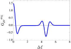
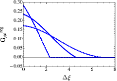
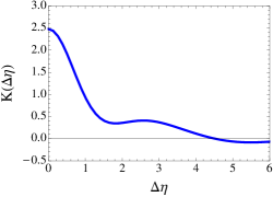
Figure 1: Left: Singular part of the contribution of a single time slice $\tau$. ${{v_{\rm s}}}^{2}=1/3$ and $\ln({\tau_{\rm f}}/\tau)=4$. In order to visualize the infinitesimally narrow singularities we “smear” the function with a Gaussian of square width $\sigma^{2}=0.1$. Center: The regular part of the correlation from 3 time slices $\tau$: $\ln({\tau_{\rm f}}/\tau)=2,4,6$. Right: Rapidity gap dependence of the particle-particle fluctuations in Eq. (9).

If the dispersion $\omega(k)$ of small fluctuations around the Bjorken solution were linear, there would only be the sound-front singularities at $\Delta\xi=2{v_{\rm s}}\ln({\tau_{\rm f}}/\tau)$ and 0. However, $\omega=i\alpha\pm\sqrt{{v_{\rm s}}^{2}k^{2}-\alpha^{2}}$ [$\alpha\equiv(1-{v_{\rm s}}^{2})/2$]. Note that the slowest mode behaves as $\omega_{-}\sim-ik^{2}$ for $k\to 0$. Correspondingly, the “wake” in Fig. 1(center) approaches a Gaussian for large time intervals $\ln(\tau_{f}/\tau)$. Although diffusion-like in appearance, this mode is present even without dissipation.

The main effect of viscosity is, as usual, to smear the sound-front singularity with a Gaussian of width which grows with time interval between ${\tau_{\rm f}}$ and $\tau$ (initially following diffusive law $\sigma\sim\sqrt{{\tau_{\rm f}}-\tau}$):

$$\sigma^{2}=\frac{\nu}{\alpha}\left(\frac{1}{\tau T}-\frac{1}{{\tau_{\rm f}}T_{\rm f}}\right)\,.$$ (8)

Finally, we translate fluctuations of hydrodynamic variables to observable fluctuations of particle distributions $dN/d\eta$ using the Cooper-Frye freezeout formalism. It takes into account the fact that particles within a given local subvolume at Bjorken rapidity $\xi$ have kinematic rapidities $\eta$ which are thermally spread around $\xi$. The result can be presented in the following form:

$$\left\langle\,\delta\frac{dN}{d\eta_{1}}\,\delta\frac{dN}{d\eta_{2}}\,\right\rangle\left\langle\,\frac{dN}{d\eta}\,\right\rangle^{-1}=\frac{45{d_{\rm s}}}{4\pi^{4}N_{\rm eff}(T_{0})}\,\frac{{\nu}}{{T_{\rm f}}{\tau_{\rm f}}}\left(\frac{{T_{0}^{2}}}{{T_{\rm f}}^{2}}\right)^{{v_{\rm s}}^{\!-2}-2}K(\Delta\eta)\,,$$ (9)

where we separated the dependence on rapidity gap $\Delta\eta=\eta_{1}-\eta_{2}$ into a factor $K(\Delta\eta)$. This factor does not depend on other parameters such as initial time and temperature $\tau_{0}$, $T_{0}$, the effective number of degrees of freedom defined via $s(T)=2\pi^{2}N_{\rm eff}(T)T^{3}/45$ and the mass degeneracy of the observed species ${d_{\rm s}}$ (e.g., 2 for charged pions). It does depend on the ratio of the particle mass and the freezeout temperature and for pions at ${T_{\rm f}}=150$ MeV it is plotted in Fig. 1(right).

We conclude by describing a qualitative picture of the two-particle correlations as a function of rapidity separation which may be helpful in disentangling the two major contributions to correlations: initial state fluctuations and hydrodynamic noise. The initial state fluctuations, being fluctuations of the two-dimensional density of the colliding Lorentz-contracted nuclear “pancakes”, create correlations which are largely independent of $\Delta\eta$ and stretch over the whole rapidity interval between spectator fragments. In contrast, hydrodynamic fluctuations are local, and it takes time for them to spread over larger $\Delta\eta$. The effect of the hydrodynamic noise is strongest at small $\Delta\eta\lesssim 1$ leading to a characteristic thermal peak (see Fig. 1(right)). At larger $\Delta\eta$ the hydrodynamic fluctuations induce correlations whose strength decreases with $\Delta\eta$ and vanishes beyond the sound horizon at $2{v_{\rm s}}\ln({\tau_{\rm f}}/\tau_{0})$. At such large $\Delta\eta$ the correlation should reach a plateau set by initial state fluctuations.

The magnitude of the noise-induced long-range correlations is proportional to viscosity, Eq. (9). This fact could potentially be used to measure or constrain the value of this important transport coefficient by studying the $\Delta\eta$ dependence of the correlations.

One can extend this analysis to the dependence of the correlations on both rapidity and azimuthal angle separation ($\Delta\eta$ and $\Delta\phi$) in a way similar to the $\Delta\phi$-only dependence analysis in Ref.[8]. This work is in progress (see T. Springer’s contribution to these proceedings, [9]). Experimental data on $\Delta\eta$, $\Delta\phi$ dependence of fluctuations, or, upon Fourier transform with respect to $\Delta\phi$, the $\Delta\eta$ dependence of $v_{nn}(\Delta\eta)$ could be compared to such a theoretical analysis. Of course, a more realistic (e.g., 3d event-by-event hydro [10]) simulation may be necessary to enable a quantitative comparison and to determine or constrain the value of the viscosity.

This work was supported by the U.S. DOE Grants No. DE-FG02-87ER40328 (JIK), DE-FG02-05ER41367 (BM), and DE-FG02-01ER41195 (MS).

References

- [1] H. Agakishiev et al. [STAR Collaboration], Phys. Lett. B 704, 467 (2011) [arXiv:1106.4334 [nucl-ex]].
- [2] K. Aamodt et al. [ALICE Collaboration], Phys. Lett. B 708, 249 (2012) [arXiv:1109.2501 [nucl-ex]].
- [3] S. Chatrchyan et al. [CMS Collaboration], Eur. Phys. J. C 72, 2012 (2012) [arXiv:1201.3158 [nucl-ex]].
- [4] G. Aad et al. [ATLAS Collaboration], Phys. Rev. C 86, 014907 (2012) [arXiv:1203.3087 [hep-ex]].
- [5] B. Alver and G. Roland, Phys. Rev. C 81, 054905 (2010).
- [6] J. I. Kapusta, B. Muller and M. Stephanov, Phys. Rev. C 85, 054906 (2012) [arXiv:1112.6405 [nucl-th]].
- [7] L. D. Landau and E. M. Lifshitz, Statistical Physics: Part 2, Pergamon Press, Oxford (1980).
- [8] P. Staig and E. Shuryak, Phys. Rev. C 84, 044912 (2011) [arXiv:1105.0676 [nucl-th]].
- [9] T. Springer and M. Stephanov, arXiv:1210.5179 [nucl-th].
- [10] B. Schenke, S. Jeon and C. Gale, Phys. Rev. Lett. 106, 042301 (2011).