A Posteriori Error Control for a Quasicontinuum Approximation of a Periodic Chain

Abstract.

We consider a 1D periodic atomistic model, for which we formulate and analyze an adaptive variant of a quasicontinuum method. We establish a posteriori error estimates for the energy norm and for the energy, based on a posteriori residual and stability estimates. We formulate adaptive mesh refinement algorithms based on these error estimators. Our numerical experiments indicate optimal convergence rates of these algorithms.

1. Introduction

Quasicontinuum (QC) methods, or more generally, atomistic-to-continuum coupling (a/c) methods, are a class of multiscale methods for coupling an atomistic model of a solid with a continuum model. These methods have been widely employed in atomistic simulations, where a fully atomistic model would result in prohibitive computational cost but is required in certain regions of interest (typically neighbourhoods of crystal defects) to achieve the desired degree of accuracy. A continuum model is applied to reduce the cost of the computation of the elastic far-fields. We refer to the recent review articles [13, 14] for introductions to QC methods.

In this paper we present an a posteriori error analysis of a simplified variant of the energy-based QC approximation proposed in [26].

Considerable effort has been devoted to the a priori error analysis of QC methods [11, 12, 22, 7, 6, 18, 21, 27, 19, 15, 10]. A posteriori error control has received comparatively little attention: Arndt and Luskin use a goal-oriented approach for the a posteriori error estimates for the QC approximation of a Frenkel-Kontorova model [2, 3, 1]. The estimates are used to optimize the choice of the atomistic region and the finite element mesh in the continuum region. Prudhomme et al. [24] also use the goal-oriented approach to provide a posteriori error control for the original energy-based QC approximation [17], which is inconsistent. Both of these approaches require the use of the solutions of dual problems. In [22] a posteriori error bounds for an energy norm are derived, using a similar approach as in the present work. However, the QC method analyzed in [22] does not contain an approximation of the stored energy and its 2D/3D version is therefore not a computationally efficient method.

In the present work, we use the residual-based approach [28, Chapter 2], which is well established in the finite element approximation of partial differential equations, to derive a posteriori error bounds for the energy-norm and for the energy itself. What distinguishes our setting from the classical one, are two particular features: 1. the model approximation (“variational crime”) is fundamentally different than quadrature approximations; 2. it is possible to adapt the mesh to a degree that the residual vanishes exactly in certain regions of interest (the atomistic region). Our work extends [18], which considers a simplified setting.

We do not tackle the question of model and mesh adaptivity for defect nucleation, but focus only on automatically choosing the size of the atomistic region and the finite element mesh in the continuum region. In many applications, a defect is inserted into the crystal before the computation, or it is known a priori where a defect will nucleate. An extension of our work to include defect nucleation would be valuable, but cannot be pursued in the simplified 1D setting we are considering here.

1.1. Outline

In Section 2 we introduce a 1D atomistic model problem, which mimics the behaviour of crystal defects in 2D/3D. Moreover, we review the construction of a QC method to efficiently approximate its solutions, and introduce the notation that will be used throughout the paper.

In Section 3, we derive a residual estimate for the QC method in a discrete negative Sobolev norm. In Section 4, we present an a posteriori stability result. In Section 5, we combine the residual estimate and the stability result to give a posteriori error estimates for the deformation gradient and for the energy.

In Section 6, we describe three mesh refinement algorithms based on our a posteriori error analysis and on previous a priori error estimates, and present a numerical example to illustrate the performance of these algorithms.

2. Model Problem and QC Approximation

2.1. Atomistic Model

Following previous works [7, 18, 23] we formulate a model problem in a discrete periodic domain containing $2N$ atoms, where $N\in\mathbb{N}$. Let $F>0$ denote a macroscopic stretch and $\varepsilon=1/(2N)$ the lattice spacing, both of which we fix throughout. We define the displacement and deformation spaces, respectively, by

$$\mathcal{U}^{\varepsilon}:=~{} \big{\{}u\in\mathbb{R}^{\mathbb{Z}}:u_{\ell+2N}=u_{\ell},\text{ and }u_{0}=0\big{\}},\quad\text{and}$$

$$\mathcal{Y}^{\varepsilon}:=~{} \big{\{}y\in\mathbb{R}^{\mathbb{Z}}:y_{\ell+2N}=F+y_{\ell},\text{ and }y_{0}=0\big{\}}.$$

In particular, we observe that $y\in\mathcal{Y}^{\varepsilon}$ if and only if $y=Fx+u$ for some $u\in\mathcal{U}^{\varepsilon}$.

The stored energy (per period) of an admissible deformation $y\in\mathcal{Y}^{\varepsilon}$ is given by

$$\mathcal{E}_{\rm a}(y):=\varepsilon\sum_{\ell=-N+1}^{N}\phi(y_{\ell}^{\prime})+\varepsilon\sum_{\ell=-N+1}^{N}\phi(y_{\ell-1}^{\prime}+y_{\ell}^{\prime}),$$

where $y_{\ell}^{\prime}:=\varepsilon^{-1}(y_{\ell}-y_{\ell-1})$ and we note that $y_{\ell-1}^{\prime}+y_{\ell}^{\prime}=\varepsilon^{-1}(y_{\ell}-y_{\ell-2})$ is a second-neighbour difference, and where $\phi\in C^{3}(0,+\infty)$ is a Lennard-Jones type interaction potential. We assume throughout that there exists $r_{\ast}>0$ such that $\phi$ is convex in $(0,r_{\ast})$ and concave in $(r_{\ast},+\infty)$.

Given a periodic dead load $f\in C^{0}(\mathbb{R}),f(x+1)=f(x)$, we define the external energy (per period) by

$$-\langle f,u\rangle_{\varepsilon}:=-\varepsilon\sum_{\ell=-N+1}^{N}f_{\ell}u_{\ell},$$ (2.1)

where $u=y-Fx$ . Thus, the total energy (per period) under a deformation $y\in\mathcal{Y}^{\varepsilon}$ is given by

$$E_{\rm a}(y):=\mathcal{E}_{\rm a}(y)-\langle f,y-Fx\rangle_{\varepsilon}.$$

We wish to compute

$$y_{\rm a}\in{\rm argmin}E_{\rm a}(\mathcal{Y}^{\varepsilon}),$$ (2.2)

where ${\rm argmin}$ denotes the set of local minimizers.

Remark 1. 1. Since the internal energy is translation invariant, our choice $u_{0}=0$ (instead of the more common constraint $\sum_{\ell=-N+1}^{N}u_{\ell}=0$) does not alter the problem but simplifies the treatment of external forces in Sections 3.2 and 3.4.

2. The external energy (2.1) can be thought of as the linearisation of a nonlinear external energy about the state $Fx$.

3. We have included the external forces primarily to render the problem non-trivial. In realistic applications in 2D/3D, defects or forces applied on a boundary are the cause of deformation of the crystal, however, in 1D such complex behaviour cannot be described directly. ∎

2.2. Notation for lattice functions

Throughout, we identify a lattice function $v\in\mathbb{R}^{\mathbb{Z}}$ with its continuous and piecewise affine interpolant with nodal values $v(\varepsilon\ell)=v_{\ell}$. Vice-versa, if $g\in C^{0}(\mathbb{R})$ then we always identify it with its vectors of nodal values $(g_{\ell})_{\ell\in\mathbb{Z}}=(g(\varepsilon\ell))_{\ell\in\mathbb{Z}}$.

Let $\mathcal{D}$ be a subset of $\mathbb{Z}$. For a vector $v\in\mathbb{R}^{\mathbb{Z}}$, we define

$$\|v\|_{\ell^{p}_{\varepsilon}(\mathcal{D})}:=\left\{\begin{array}[]{l l}\Big{(}\sum_{\ell\in\mathcal{D}}\varepsilon|v_{\ell}|^{p}\Big{)}^{1/p},&1\leq p<\infty,\\ \max_{\ell\in\mathcal{D}}|v_{\ell}|,&p=\infty.\end{array}\right.$$

If the label $\mathcal{D}$ is omitted, then we understand this to mean $\mathcal{D}=\{-N+1,\dots,N\}$.

We define the first discrete derivatives $v_{\ell}^{\prime}:=(v_{\ell}-v_{\ell-1})/\varepsilon$. It is then straightforward to see that, if at the same time we identify $v^{\prime}$ with the pointwise derivative, then $\|v^{\prime}\|_{L^{p}(-1/2,1/2)}=\|v^{\prime}\|_{\ell^{p}_{\varepsilon}}$.

We equip the space $\mathcal{U}^{\varepsilon}$ with the discrete Sobolev norm (recall that $u_{0}=0$)

$$\|v\|_{\mathcal{U}^{1,2}}:=\|v^{\prime}\|_{L^{2}(-1/2,1/2)}\quad\text{ for }v\in\mathcal{U}^{\varepsilon}.$$

The norm on the dual $(\mathcal{U}^{\varepsilon})^{*}$ is defined by

$$\|T\|_{\mathcal{U}^{-1,2}}:=\sup_{\begin{subarray}{c}v\in\mathcal{U}^{\varepsilon}\\ \|v\|_{\mathcal{U}^{1,2}}=1\end{subarray}}T[v].$$

2.3. Finite element notation

To construct the QC approximation in the next section, we first define some convenient notation. Let $\Omega:=[-1/2,1/2]$ denote the computational cell. We choose an atomistic region $\Omega_{\rm a}\subset\Omega$, where atomistic accuracy is required, and we define the continuum region by $\Omega_{\rm c}:=\Omega\setminus\Omega_{\rm a}$. We will also use the periodic extension of $\Omega_{\rm c}$, denoted by $\Omega_{\rm c}^{\#}:=(\Omega_{\rm c}+\mathbb{Z})$.

We assume throughout that $\Omega_{\rm a}$ is an open interval $(L_{\rm a},R_{\rm a})$ with $-1/2<L_{\rm a}<R_{\rm a}<1/2$. All our results (with the exception of Section 3.4) can be extended without difficulty to the case when $\Omega_{\rm a}$ consists of a finite union of open intervals.

Let $\{T_{k}^{h}\}_{k\in\mathbb{Z}}$ be a partition of $\mathbb{R}$ into closed intervals with $T_{k}^{h}=[x^{h}_{k-1},x^{h}_{k}]$, where $x^{h}_{k}>x^{h}_{k-1}$ are the nodes of the partition. We assume, without loss of generality, that $x_{1}^{h}$ is the left-most node and $x_{K}^{h}$ the right-most nodes in the interval $(-1/2,1/2]$.

The length of an element is denoted by $h_{k}:=|T_{k}^{h}|:=x^{h}_{k}-x^{h}_{k-1}$. The space of continuous piecewise affine functions with respect to the partition $\mathcal{T}^{h}$ is denoted by $\mathcal{P}_{1}(\mathcal{T}^{h})$.

We assume throughout that the partition $\mathcal{T}^{h}$ has the following properties:

• $\mathcal{T}^{h}$ is periodic: there exists $K\in\mathbb{N}$ such that $x_{k+K}^{h}=1+x_{k}^{h}$ for all $k\in\mathbb{Z}$.

• $\mathcal{T}^{h}$ has atomistic resolution in $\Omega_{\rm a}$: $\Omega_{\rm a}\cap\varepsilon\mathbb{Z}=\Omega_{\rm a}\cap\{x_{k}^{h}\}_{k\in\mathbb{Z}}$.

• The a/c interface points are finite element nodes: $\partial\Omega_{\rm a}\subset\{x^{h}_{k}\}_{k\in\mathbb{Z}}$. In particular, each element belongs entirely to either the atomistic or continuum region.

• If $T^{h}_{k}\subset\Omega_{\rm c}^{\#}$ then $|T_{k}^{h}|=h_{k}\geq 2\varepsilon$.

Property (T4) is not strictly required, but simplifies the analysis and is not a significant restriction. Note also that we have not required (except in the atomistic region) that finite element nodes must be positioned on atomic sites. Although not necessary in 1D, it somewhat simplifies mesh generation, and to some extend mimics the fact that element edges or faces in 2D/3D cannot normally be aligned with the underlying crystal lattice.

The finite element displacement and deformation spaces are defined, respectively, by

$$\mathcal{U}^{h}:=~{} \big{\{}u_{h}\in\mathcal{P}_{1}(\mathcal{T}^{h}):u_{h}(x+1)=u_{h}(x)\text{ and }u_{h}(0)=0\big{\}},\quad\text{and}$$ (2.3)

$$\mathcal{Y}^{h}:=~{} \big{\{}y_{h}\in\mathcal{P}_{1}(\mathcal{T}^{h}):y_{h}-Fx\in\mathcal{U}^{h}\big{\}}.$$ (2.4)

For $g\in C^{0}(\mathbb{R})$, we define the interpolation operator $I_{h}:C^{0}(\mathbb{R})\rightarrow\mathcal{P}_{1}(\mathcal{T}^{h})$ by

$$(I_{h}g)(x^{h}_{k}):=g(x^{h}_{k})\qquad\forall k\in\mathbb{Z}.$$ (2.5)

We note that $I_{h}:\mathcal{U}^{\varepsilon}\to\mathcal{U}^{h}$.

For future reference, we also define the micro-elements $T_{\ell}^{\varepsilon}:=((\ell-1)\varepsilon,\ell\varepsilon)$ for $\ell\in\mathbb{Z}$. Analogously, we define $I_{\varepsilon}$ to be the nodal interpolant with respect to the atomistic grid. We will require this interpolant since the mesh nodes $\{x_{k}^{h}\}_{k\in\mathbb{Z}}$ do not necessarily coincide with lattice sites.

2.4. QC Approximation

The QC approximation we analyze in this paper is the 1D variant of the ACC method described in [26]. (An earlier variant of the idea was described in [18] and a similar construction in [10]. We focus on the formulation proposed in [26] since it can be readily generalised to 2D.)

The idea of the ACC method is based on the splitting of interaction bonds. A bond is an open interval $b=(\ell\varepsilon,(\ell+j)\varepsilon)$ for $\ell\in\mathbb{Z}$ and $j\in\{1,2\}$ (since we consider only first and second neighbour interactions). Since our computational domain is $(0,1]$ the set of bonds over which the atomistic energy is defined is given by

$$\mathcal{B}:=\big{\{}(\ell\varepsilon,(\ell+j)\varepsilon):j=1,2;\ell=-N+1,\ldots,N\big{\}}.$$ (2.6)

For each bond $b=(\ell\varepsilon,(\ell+j)\varepsilon)$ we define $r_{b}:=j$.

For any open interval $\omega=(L_{\omega},R_{\omega})$ (e.g., for a bond) with length $|\omega|:=R_{\omega}-L_{\omega}>0$ we define the finite difference operator

$$D_{\omega}v:=\frac{v(R_{\omega})-v(L_{\omega})}{|\omega|}\qquad\text{for }v\in C^{0}(\mathbb{R}).$$ (2.7)

Note that, with this notation, we can rewrite $\mathcal{E}_{\rm a}(y)=\varepsilon\sum_{b\in\mathcal{B}}\phi\big{(}r_{b}D_{b}y\big{)}$.

For each bond $b$ and deformation field $y\in W^{1,\infty}(\mathbb{R})$ we define its atomistic and continuum energy contributions to the stored energy, respectively, by

$$a_{b}(y):=\frac{|b\cap\Omega_{\rm a}|}{|b|}\phi\big{(}r_{b}D_{b\cap\Omega_{\rm a}}y\big{)}\quad\text{and}\quad c_{b}(y):=\frac{1}{|b|}\int_{b\cap\Omega_{\rm c}^{\#}}\phi\big{(}r_{b}y^{\prime}(x)\big{)}\,{\rm d}x.$$

If $|b\cap\Omega_{\rm a}|=0$ then $D_{b\cap\Omega_{\rm a}}y$ is ill-defined; in that case we define $a_{b}\equiv 0$. The QC energy (the ACC energy of [26]) of a deformation field $y\in W^{1,\infty}(\mathbb{R})$ is now defined by

$$\mathcal{E}_{{\rm qc}}(y):=\varepsilon\sum_{b\in\mathcal{B}}\big{[}a_{b}(y)+c_{b}(y)\big{]}.$$ (2.8)

The key property of this definition is that it satisfies the patch test [26, Section 3.3],

$$\mathcal{E}^{\prime}_{{\rm a}}(Fx)[v_{\varepsilon}]=\mathcal{E}^{\prime}_{{\rm qc}}(Fx)[v_{h}]=0\quad\text{for all }v_{\varepsilon}\in\mathcal{U}^{\varepsilon}\text{ and }v_{h}\in\mathcal{U}^{h},\quad\forall F>0.$$ (2.9)

The external energy (per period) is given by

$$-\langle f,u_{h}\rangle_{h}:=-\int_{\Omega}I_{h}(fu_{h})\,{\rm d}x.$$ (2.10)

Note that, in the atomistic region, this reduces to the same form as (2.1). The total energy (per period) of a deformation $y_{h}\in\mathcal{Y}^{h}$ is then given by

$$E_{{\rm qc}}(y_{h}):=\mathcal{E}_{{\rm qc}}(y_{h})-\langle f,y_{h}-Fx\rangle_{h}.$$

In the QC approximation we seek

$$y_{{\rm qc}}\in{\rm argmin}\,E_{{\rm qc}}(\mathcal{Y}^{h}).$$ (2.11)

Remark 2. It is initially not obvious why the formulation (2.8) should reduce the complexity of the computation of $y_{\rm qc}$ over that of $y_{\rm a}$, since $\mathcal{E}_{\rm qc}$ is still written as a summation over all bonds. However, one can readily check (see [26] for the details), that

$$\mathcal{E}_{{\rm qc}}(y_{h})=\sum_{b\in\mathcal{B}}a_{b}(y_{h})+\int_{\Omega_{\rm c}}W(y_{h}^{\prime})\,{\rm d}x,$$

where $W(r):=\phi(r)+\phi(2r)$ is the Cauchy–Born stored energy function. This formulation requires only a sum over all bonds within the atomistic region, and a standard finite element assembly procedure to compute the energy contribution from the continuum region. Thus, the evaluation of $\mathcal{E}_{\rm qc}$ has only a computational complexity proportional to $\#\mathcal{T}^{h}$.

Analogous results hold in 2D [26]; a more involved assembly procedure is required to make the ACC method efficient in 3D [25]. ∎

3. Residual Analysis

3.1. The residual

Let $y_{\rm a}$ be a solution of the atomistic problem (2.2). It is straightforward to see that, if $y_{\rm a}^{\prime}>0$, then $\mathcal{E}_{{\rm a}}$ is differentiable at $y_{\rm a}$ and hence the first order optimality condition for (2.2) is satisfied:

$$\mathcal{E}^{\prime}_{\rm a}(y_{\rm a})[v]=\langle f,v\rangle_{\varepsilon}\qquad\forall v\in\mathcal{U}^{\varepsilon},$$ (3.1)

$$\text{where}\quad\mathcal{E}^{\prime}_{\rm a}(y_{\rm a})[v]=\varepsilon\sum_{b\in\mathcal{B}}\phi^{\prime}(r_{b}D_{b}y_{\rm a})r_{b}D_{b}v.$$ (3.2)

Similarly, if $y_{{\rm qc}}$ is a solution of the QC problem (2.11) with $y_{{\rm qc}}^{\prime}>0$ on $[-1/2,1/2]$, then it satisfies the corresponding first order optimality condition

$$\mathcal{E}^{\prime}_{{\rm qc}}(y_{{\rm qc}})[v_{h}]=\langle f,v_{h}\rangle_{h}\qquad\forall v_{h}\in\mathcal{U}^{h},$$ (3.3)

$$\text{where}\quad\mathcal{E}^{\prime}_{{\rm qc}}(y_{h})[v_{h}] =\sum_{b\in\mathcal{B}}\big{(}a^{\prime}_{b}(y_{h})[v_{h}]+c_{b}^{\prime}(y_{h})[v_{h}]\big{)}$$ (3.4)

$$=\sum_{b\in\mathcal{B}}|b\cap\Omega_{\rm a}|\phi^{\prime}(r_{b}D_{b\cap\Omega_{\rm a}}y_{h})D_{b\cap\Omega_{\rm a}}v_{h}+\sum_{b\in\mathcal{B}}\int_{b\cap\Omega_{\rm c}^{\#}}\phi^{\prime}({r_{b}y^{\prime}_{h}(x)})v_{h}^{\prime}\,{\rm d}x.$$

Let $y_{{\rm qc}}\in\mathcal{Y}^{h}$ be a solution of (2.11), then we define its residual $R\in(\mathcal{U}^{\varepsilon})^{*}$ by

$$R[v]:=E^{\prime}_{{\rm a}}(y_{{\rm qc}})[v],$$ (3.5)

Using (3.3) we can rewrite this as

$$R[v]=~{} E_{{\rm a}}^{\prime}(y_{{\rm qc}})[v]-E^{\prime}_{{\rm qc}}(y_{{\rm qc}})[I_{h}v]$$

$$=~{} \big{\{}\mathcal{E}^{\prime}_{{\rm a}}(y_{{\rm qc}})[v]-\mathcal{E}^{\prime}_{{\rm qc}}(y_{{\rm qc}})[I_{h}v]\big{\}}-\big{\{}\langle f,v\rangle_{\varepsilon}-\langle f,I_{h}v\rangle_{h}\big{\}}$$

$$=:~{} R_{\rm int}[v]+R_{\rm ext}[v],$$

where we call $R_{\rm int}$ the internal residual and $R_{\rm ext}$ the external residual. We will bound them separately in the next two sections.

3.2. Estimate for the internal residual

In this section, we analyze the internal residual $R_{\rm int}$. To state the main theorem, we define the index set of all nodes in the continuum region and a/c interface (recall that $\Omega_{\rm c}$ is closed),

$$\mathcal{K}_{\rm c}:=\big{\{}k\in\{1,\ldots,K\}:x_{k}^{h}\in\Omega_{\rm c}\big{\}}.$$ (3.6)

Theorem 1. Let $y_{h}\in\mathcal{Y}^{h}$ such that $y_{h}^{\prime}>0$ and $R_{\rm int}[v]=\mathcal{E}^{\prime}_{{\rm a}}(y_{h})[v]-\mathcal{E}^{\prime}_{{\rm qc}}(y_{h})[I_{h}v]$, then

$$\big{\|}R_{\rm int}\big{\|}_{\mathcal{U}^{-1,2}}\leq\Big{(}3\sum_{k\in\mathcal{K}_{\rm c}}\eta_{k}^{2}\Big{)}^{\frac{1}{2}}=:\eta(y_{h}),\qquad\text{where}$$ (3.7)

$$\eta_{k}^{2}:=\!\!\!\sum_{\begin{subarray}{c}b\in\mathcal{B}\\ x_{k}^{h}\in{\rm int}(b)\end{subarray}}\Big{(}\big{\|}\phi^{\prime}(r_{b}D_{b}y_{h})-\phi^{\prime}(r_{b}D_{b\cap\Omega_{\rm a}}y_{h})\big{\|}_{L^{2}(b\cap\Omega_{\rm a})}^{2}+\big{\|}\phi^{\prime}(r_{b}D_{b}y_{h})-\phi^{\prime}(r_{b}y_{h}^{\prime})\big{\|}_{L^{2}(b\cap\Omega_{\rm c}^{\#})}^{2}\Big{)}.$$

Remark 3. 1. The expressions for $\eta_{k}$ are reminiscent of the flux (or stress) jump terms that occur in the classical residual error analysis for partial differential equations. The origin in our case, is somewhat different however, and results only from the model approximation and not the finite element coarsening.

2. With some additional work, the form of the estimates $\rho_{k}$ can be turned into element contributions and further simplified by computing more explicit representations. ∎

Proof.

Let $v_{h}:=I_{h}v$. From (3.2) and (3.4) we obtain

$$R_{\rm int}[v]= \sum_{b\in\mathcal{B}}\Big{\{}|b|\phi^{\prime}(r_{b}D_{b}y_{h})D_{b}v-|b\cap\Omega_{\rm a}|\phi^{\prime}(r_{b}D_{b\cap\Omega_{\rm a}}y_{h})D_{b\cap\Omega_{\rm a}}v_{h}-\int_{b\cap\Omega_{\rm c}^{\#}}\phi^{\prime}(r_{b}y_{h}^{\prime})v_{h}^{\prime}\,{\rm d}x\Big{\}}.$$ (3.8)

We subtract and add the terms

$$\sum_{b\in\mathcal{B}}|b\cap\Omega_{\rm a}|\phi^{\prime}(r_{b}D_{b\cap\Omega_{\rm a}}y_{h})D_{b\cap\Omega_{\rm a}}v\quad\text{ and }\quad\sum_{b\in\mathcal{B}}\int_{b\cap\Omega_{\rm c}^{\#}}\phi^{\prime}({r_{b}y^{\prime}_{h}(x)})v^{\prime}\,{\rm d}x$$

to split $R_{\rm int}$ into three components,

$$R_{\rm int}[v]$$

$$=~{} \sum_{b\in\mathcal{B}}\bigg{\{}|b|\phi^{\prime}(r_{b}D_{b}y_{h})D_{b}v-|b\cap\Omega_{\rm a}|\phi^{\prime}(r_{b}D_{b\cap\Omega_{\rm a}}y_{h})D_{b\cap\Omega_{\rm a}}v-\int_{b\cap\Omega_{\rm c}^{\#}}\phi^{\prime}({r_{b}y^{\prime}_{h}(x)})v^{\prime}\,{\rm d}x\bigg{\}}$$

$$+\sum_{b\in\mathcal{B}}|b\cap\Omega_{\rm a}|\phi^{\prime}(r_{b}D_{b\cap\Omega_{\rm a}}y_{h})\big{(}D_{b\cap\Omega_{\rm a}}v-D_{b\cap\Omega_{\rm a}}v_{h}\big{)}$$

$$+\sum_{b\in\mathcal{B}}\int_{b\cap\Omega_{\rm c}^{\#}}\phi^{\prime}({r_{b}y^{\prime}_{h}(x)})\big{(}v^{\prime}-v_{h}^{\prime}\big{)}\,{\rm d}x$$

$$=:~{} R_{1}[v]+R_{2}[v]+R_{3}[v].$$ (3.9)

We will show that $R_{2}\equiv R_{3}\equiv 0$ and estimate $R_{1}$.

For $R_{2}$ this follows simply from the fact that $v_{h}=v$ in $\Omega_{\rm a}$ and hence $D_{b\cap\Omega_{\rm a}}v=D_{b\cap\Omega_{\rm a}}v_{h}$ for all $b\in\mathcal{B}$ such that $|b\cap\Omega_{\rm a}|>0$.

For $R_{3}$, following the computations in [26, Section 3.2], we obtain

$$R_{3}[v]=\int_{\Omega_{\rm c}}W^{\prime}(y_{h}^{\prime})(v^{\prime}-v_{h}^{\prime})\,{\rm d}x,$$

where $W(r)=\phi(r)+\phi(2r)$. Since $v(x_{k}^{h})=v_{h}(x_{k}^{h})$ for all $k\in\mathbb{Z}$ and since $W^{\prime}(y_{h}^{\prime})$ is constant on each element $T_{k}^{h}$ it follows that $R_{3}\equiv 0$.

Finally, we turn to the analysis of $R_{1}=\sum_{b\in\mathcal{B}}R_{1}^{b}$, where we define

$$R_{1}^{b}[v]:=~{} |b|\phi^{\prime}(r_{b}D_{b}y_{h})D_{b}v-|b\cap\Omega_{\rm a}|\phi^{\prime}(r_{b}D_{b\cap\Omega_{\rm a}}y_{h})D_{b\cap\Omega_{\rm a}}v-\int_{b\cap\Omega_{\rm c}^{\#}}\phi^{\prime}({r_{b}y^{\prime}_{h}(x)})v^{\prime}\,{\rm d}x.$$

Using the fact that $|\omega|D_{\omega}v=\int_{\omega}v^{\prime}\,{\rm d}x$ we obtain

$$R_{1}^{b}[v]=~{} \int_{b}\phi^{\prime}(r_{b}D_{b}y_{h})v^{\prime}\,{\rm d}x-\int_{b\cap\Omega_{\rm a}}\phi^{\prime}(r_{b}D_{b\cap\Omega_{\rm a}}y_{h})v^{\prime}\,{\rm d}x-\int_{b\cap\Omega_{\rm c}^{\#}}\phi^{\prime}({r_{b}y^{\prime}_{h}(x)})v^{\prime}\,{\rm d}x$$

$$=~{} \int_{b\cap\Omega_{\rm a}}\big{[}\phi^{\prime}(r_{b}D_{b}y_{h})-\phi^{\prime}(r_{b}D_{b\cap\Omega_{\rm a}}y_{h})\big{]}v^{\prime}\,{\rm d}x+\int_{b\cap\Omega_{\rm c}^{\#}}\big{[}\phi^{\prime}(r_{b}D_{b}y_{h})-\phi^{\prime}(r_{b}y_{h}^{\prime})\big{]}v^{\prime}\,{\rm d}x.$$

If $b\subset\Omega_{\rm a}$, then $b\cap\Omega_{\rm a}=b$ and $|b\cap\Omega_{\rm c}|=0$, and hence $R_{1}^{b}=0$. Similarly, if $b\subset T_{k}^{h}\subset\Omega_{\rm c}^{\#}$, then $D_{b}y_{h}=y_{h}^{\prime}|_{T_{k}^{h}}$ and $|b\cap\Omega_{\rm a}|=0$ and hence $R_{1}^{b}=0$. Thus, we observe that only bonds crossing continuum element boundaries, or the atomistic/continuum interface, contribute to the residual. These are precisely the points contained in $\mathcal{K}_{\rm c}$. In particular, we obtain

$$R_{1}[v]=\sum_{k\in\mathcal{K}_{\rm c}}\sum_{\begin{subarray}{c}b\in\mathcal{B}\\ x_{k}^{h}\in{\rm int}(b)\end{subarray}}R_{1}^{b}[v],$$ (3.10)

where we used the fact that no bond can cross more than one point $x_{k}^{h}\in\mathcal{K}_{\rm c}$ due to our assumption that all elements have at least length $2\varepsilon$.

From the definition of $R_{1}^{b}$, and applying two Cauchy–Schwarz inequalities, it is straightforward to estimate

$$\big{|}R_{1}^{b}[v]\big{|}\leq\Big{(}\, \big{\|}\phi^{\prime}(r_{b}D_{b}y_{h})-\phi^{\prime}(r_{b}D_{b\cap\Omega_{\rm a}}y_{h})\big{\|}_{L^{2}(b\cap\Omega_{\rm a})}^{2}$$

$$\qquad+\big{\|}\phi^{\prime}(r_{b}D_{b}y_{h})-\phi^{\prime}(r_{b}y_{h}^{\prime})\big{\|}_{L^{2}(b\cap\Omega_{\rm c}^{\#})}^{2}\Big{)}^{1/2}\|v^{\prime}\|_{L^{2}(b)},$$

and after applying another Cauchy–Schwarz inequality,

$$\Big{|}\sum_{\begin{subarray}{c}b\in\mathcal{B}\\ x_{k}^{h}\in{\rm int}(b)\end{subarray}}R_{1}^{b}[v]\Big{|}\leq\, \eta_{k}\,\Big{(}\sum_{\begin{subarray}{c}b\in\mathcal{B}\\ x_{k}^{h}\in{\rm int}(b)\end{subarray}}\|v^{\prime}\|_{L^{2}(b)}^{2}\Big{)}^{1/2},$$

where $\eta_{k}$ is defined in (3.7).

Combing our foregoing estimates, we arrive at

$$R_{1}[v]\leq\, \sum_{k\in\mathcal{K}_{\rm c}}\eta_{k}\,\Big{(}\sum_{\begin{subarray}{c}b\in\mathcal{B}\\ x_{k}^{h}\in{\rm int}(b)\end{subarray}}\|v^{\prime}\|_{L^{2}(b)}^{2}\Big{)}^{1/2}$$

$$\leq\, \Big{(}\sum_{k\in\mathcal{K}_{\rm c}}\eta_{k}^{2}\Big{)}^{1/2}\,\Big{(}\sum_{k\in\mathcal{K}_{\rm c}}\sum_{\begin{subarray}{c}b\in\mathcal{B}\\ x_{k}^{h}\in{\rm int}(b)\end{subarray}}\|v^{\prime}\|_{L^{2}(b)}^{2}\Big{)}^{1/2},$$

and we are only left to estimate the sums involving the test function.

To that end, we simply note that, due to (T4), for any fixed point $x\in(-1/2,1/2]$, the maximal number of bonds appearing in the sum on the left-hand side below and crossing $x$ is three; hence,

$$\sum_{k\in\mathcal{K}_{\rm c}}\sum_{\begin{subarray}{c}b\in\mathcal{B}\\ x_{k}^{h}\in{\rm int}(b)\end{subarray}}\|v^{\prime}\|_{L^{2}(b)}^{2}\leq 3\|v^{\prime}\|_{L^{2}}^{2}.$$

This concludes the proof. ∎

3.3. Estimate of the external residual

We now turn to the estimate of the residual of the external energy, which was defined as

$$R_{\rm ext}[v]=\langle f,v\rangle_{\varepsilon}-\langle f,I_{h}v\rangle_{h}=\int_{\Omega}\big{[}I_{\varepsilon}(fv)-I_{h}(fI_{h}v)\big{]}\,{\rm d}x.$$ (3.11)

We outline the key points of the argument for estimating $R_{\rm ext}$, before stating the result.

We define a slightly extended continuum region,

$$\tilde{\Omega}_{\rm c}:=\bigcup\big{\{}T_{\ell}^{\varepsilon}:|T_{\ell}^{\varepsilon}\cap\Omega_{\rm c}|>0\big{\}};$$

then $I_{\varepsilon}(fv)=I_{h}(fI_{h}v)$ in $\Omega_{\rm a}\setminus\tilde{\Omega}_{\rm c}$, and therefore

$$R_{\rm ext}[v]=\, \int_{\tilde{\Omega}_{\rm c}}\big{[}I_{\varepsilon}(fv)-I_{h}(fI_{h}v)\big{]}\,{\rm d}x$$

$$=\, \int_{\tilde{\Omega}_{\rm c}}\big{[}I_{\varepsilon}(fv)-fv\big{]}\,{\rm d}x+\int_{\tilde{\Omega}_{\rm c}}\big{[}fv-fI_{h}v\big{]}\,{\rm d}x+\int_{\tilde{\Omega}_{\rm c}}\big{[}fI_{h}v-I_{h}(fI_{h}v)\big{]}\,{\rm d}x$$

$$=:\, R_{1}[v]+R_{2}[v]+R_{3}[v].$$ (3.12)

The three terms can be estimated using standard interpolation error results, hence we only give a brief outline of the proof of the resulting bound.

Proposition 2. Let $f\in C^{2}(\tilde{\Omega}_{c})$, then

$$\|R_{\rm ext}\|_{\mathcal{U}^{-1,2}}\leq\eta^{f}+\eta^{q},$$ (3.13)

where the error due to external forces $\eta^{f}$ and the “quadrature error” $\eta^{q}$ are, respectively, defined as follows: for $*\in\{f,q\}$,

$$(\eta^{*})^{2}:=\, \sum_{\begin{subarray}{c}k\in\{1,\dots,K\}\\ T_{k}^{h}\subset\tilde{\Omega}_{\rm c}\end{subarray}}(\eta_{k}^{*})^{2},$$

$$\text{where}\qquad(\eta_{k}^{f})^{2}:=\, {\textstyle\frac{h_{k}^{2}}{\pi^{2}}}\|f\|_{L^{2}(T_{k}^{h})}^{2},$$

$$\text{and}\qquad(\eta_{k}^{q})^{2}:=\, (\varepsilon^{4}+h_{k}^{4})\|f^{\prime}\|_{L^{2}(T_{k}^{h})}^{2}+{{\textstyle\frac{(\varepsilon^{4}+h_{k}^{4})}{4\pi^{2}}}}\|f^{\prime\prime}\|_{L^{2}(T_{k}^{h})}^{2}.$$

Remark 4. 1. Note that there is an error contribution from the atomistic region, due to the fact that in the elements touching the a/c interface, the “quadrature” approximation of the external forces is not exact. For the purpose of mesh refinement, we count this error towards the neighbouring elements in the continuum region.

2. An alternative residual estimate that does not use $f\in C^{2}(\tilde{\Omega}_{\rm c})$, but only the discrete setting, is presented in [29]. This requires a much more involved argument. ∎

Proof.

From (3.12) we obtain

$$R_{\rm ext}[v]=R_{1}[v]+R_{2}[v]+R_{3}[v].$$

Applying standard interpolation error estimates (see, e.g., [5, 4]) on elements $T_{\ell}^{\varepsilon},T_{k}^{h}$, we obtain

$$\int_{T^{\varepsilon}_{\ell}}\big{[}I_{\varepsilon}(fv)-fv\big{]}\,{\rm d}x\leq~{} {\textstyle\frac{1}{4}}\|\varepsilon^{2}f^{\prime\prime}\|_{L^{2}(T^{\varepsilon}_{\ell})}\|v\|_{L^{2}(T^{\varepsilon}_{\ell})}+{\textstyle\frac{1}{2}}\|\varepsilon^{2}f^{\prime}\|_{L^{2}(T^{\varepsilon}_{\ell})}\|v^{\prime}\|_{L^{2}(T^{\varepsilon}_{\ell})},$$

$$\int_{T^{h}_{k}}\big{[}fv-fI_{h}v\big{]}\,{\rm d}x\leq~{} {\textstyle\frac{1}{\pi}}\|h_{k}f\|_{L^{2}(T^{h}_{k})}\|v^{\prime}\|_{L^{2}(T^{h}_{k})},\quad\text{and}$$

$$\int_{T^{h}_{k}}\big{[}I_{h}(fv)-fI_{h}v\big{]}\,{\rm d}x\leq~{} {\textstyle\frac{1}{4}}\|h_{k}^{2}f^{\prime\prime}\|_{L^{2}(T^{h}_{k})}\|I_{h}v\|_{L^{2}(T^{h}_{k})}+{\textstyle\frac{1}{2}}\|h_{k}^{2}f^{\prime}\|_{L^{2}(T^{h}_{k})}\|I_{h}v^{\prime}\|_{L^{2}(T^{h}_{k})}.$$

Summing over all elements, applying the Cauchy–Schwarz inequality, and defining $h(x):=h_{k}$ for $x\in T_{k}^{h}$,

$$R_{1}[v]\leq\, {\textstyle\frac{\varepsilon^{2}}{4}}\|f^{\prime\prime}\|_{L^{2}(\tilde{\Omega}_{\rm c})}\,\|v\|_{L^{2}}+{\textstyle\frac{\varepsilon^{2}}{2}}\|f^{\prime}\|_{L^{2}(\tilde{\Omega}_{\rm c})}\,\|v^{\prime}\|_{L^{2}},$$

$$R_{2}[v]\leq\, {\textstyle\frac{1}{\pi}}\|hf\|_{L^{2}(\tilde{\Omega}_{\rm c})}\,\|v^{\prime}\|_{L^{2}},\qquad\text{and}$$

$$R_{3}[v]\leq\, {\textstyle\frac{1}{4}}\|h^{2}f^{\prime\prime}\|_{L^{2}(\tilde{\Omega}_{\rm c})}\,\|I_{h}v\|_{L^{2}}+{\textstyle\frac{1}{2}}\|h^{2}f^{\prime}\|_{L^{2}(\tilde{\Omega}_{\rm c})}\,\|I_{h}v^{\prime}\|_{L^{2}}.$$

We now use the estimates (which exploit the fact that $I_{h}v^{\prime}$ is the $L^{2}$-orthogonal projection of $v^{\prime}$ onto piecewise constants)

$$\|v\|_{L^{2}}\leq{{\textstyle\frac{1}{\pi}}}\|v^{\prime}\|_{L^{2}},\quad\|I_{h}v^{\prime}\|_{L^{2}}\leq\|v^{\prime}\|_{L^{2}},$$

and $$\|I_{h}v\|_{L^{2}}\leq{\textstyle\frac{1}{\pi}}\|I_{h}v^{\prime}\|_{L^{2}}\leq{\textstyle\frac{1}{\pi}}\|v^{\prime}\|_{L^{2}},$$

to deduce that

$$R_{\rm ext}[v]=\, R_{1}[v]+R_{2}[v]+R_{3}[v]$$

$$\leq\, {\textstyle\frac{1}{\pi}}\|hf\|_{L^{2}(\tilde{\Omega}_{\rm c})}\|v^{\prime}\|_{L^{2}}+\Big{(}{\textstyle\frac{1}{4\pi^{2}}}\|(\varepsilon^{2}+h^{2})f^{\prime\prime}\|_{L^{2}(\tilde{\Omega}_{\rm c})}^{2}+\|(\varepsilon^{2}+h^{2})f^{\prime}\|_{L^{2}(\tilde{\Omega}_{\rm c})}^{2}\Big{)}^{1/2}\|v^{\prime}\|_{L^{2}}.$$

The result follows by splitting the norms inside the brackets over elements. ∎

3.4. External residual estimate for singular forces

In our numerical experiments in Section 6 we shall employ an external force that behaves like $|f(x)|\sim|x|^{-1}$ near $x=0$ (we use the “singularity” in the force to mimic a defect). Let us suppose that we also have $|f^{\prime}(x)|\sim|x|^{-2}$ and $|f^{\prime\prime}(x)|\sim|x|^{-3}$ near the origin. We now give a formal motivation why the quadrature estimates employed in Proposition 3.3 are inadequate in this situation.

Applying the quadrature estimates to such a force field, we obtain

$$\eta_{k}^{q}\approx h_{k}^{2}\|f^{\prime}\|_{L^{2}(T_{k}^{h})}+h_{k}^{2}\|f^{\prime\prime}\|_{L^{2}(T_{k}^{h})}\approx h_{k}^{5/2}|x_{k}^{h}|^{-3/2}+h_{k}^{5/2}|x_{k}^{h}|^{-5/2}.$$

We notice that, for $T_{k}^{h}$ near the origin, $\|f^{\prime\prime}\|_{L^{2}(T_{k}^{h})}\approx|x_{k}^{h}|^{-1}\|f^{\prime}\|_{L^{2}(T_{k}^{h})}$. Moreover, the quadrature estimate is $O(1)$ and cannot be controlled. By contrast,

$$\eta_{k}^{f}\approx h_{k}^{3/2}|x_{k}^{h}|^{-1},$$

from which we conclude that $h_{k}^{2}\|f^{\prime}\|_{L^{2}(T_{k}^{h})}$ is dominated by $\eta_{k}^{f}$, but that $\eta_{k}^{f}$ is itself dominated by $h_{k}^{2}\|f^{\prime\prime}\|_{L^{2}(T_{k}^{h})}$.

The origin of this undesirable effect is the (ab-)use of the Poincaré inequality in the proof of Proposition 3.3. In the remainder of this section, we shall remedy the situation by replacing the standard Poincaré inequality with a weighted variant. This approach is inspired by [20].

Lemma 3. Let $\tilde{\Omega}_{\rm c}$ be defined as in Section 3.3, and let $w(x):=x\log^{2}(x)$, then

$$\|w^{-1}v\|_{L^{2}(\tilde{\Omega}_{\rm c})}\leq{\textstyle\frac{1}{\log 2}}\|v^{\prime}\|_{L^{2}}\qquad\forall v\in H^{1}(\Omega),v(0)=0,$$

Proof.

We begin by noting that

$$|v(x)|\leq|x|^{1/2}\|v^{\prime}\|_{L^{2}}\quad\text{for all }x\in\Omega.$$

Hence, we can estimate

$$\int_{\tilde{R}_{\rm a}}^{1/2}|w^{-1}v(x)|^{2}\,{\rm d}x\leq\|v^{\prime}\|_{L^{2}(0,1/2)}^{2}\int_{\tilde{R}_{\rm a}}^{1/2}\frac{1}{x\log^{2}(2x)}\,{\rm d}x.$$

Since $(\log^{-1}(x))^{\prime}=-(x\log^{2}(x))^{-1}$ we obtain

$$\int_{\tilde{R}_{\rm a}}^{1/2}|w^{-1}v(x)|^{2}\,{\rm d}x\leq{\textstyle\frac{1}{\log(2)}}\|v^{\prime}\|_{L^{2}(0,1/2)}^{2}.$$

Applying an analogous argument in the left half of the domain, we obtain the stated estimate. ∎

We now apply this estimate to obtain an alternative external residual estimate.

Proposition 4. Let $f\in C^{2}(\tilde{\Omega}_{c})$, then

$$\|R_{\rm ext}\|_{\mathcal{U}^{-1,2}}\leq\eta^{f}+\hat{\eta}^{q},$$ (3.14)

where $\eta^{f}$ is defined in (3.13) and $\hat{\eta}^{q}$ is defined as follows:

$$(\hat{\eta}^{q})^{2}:=\, \sum_{\begin{subarray}{c}k\in\{1,\dots,K\}\\ T_{k}^{h}\subset\tilde{\Omega}_{\rm c}\end{subarray}}(\hat{\eta}^{q}_{k})^{2},$$

$$\text{where}\qquad(\hat{\eta}_{k}^{q})^{2}:=\, (\varepsilon^{4}+h_{k}^{4})\|f^{\prime}\|_{L^{2}(T_{k}^{h})}^{2}+{\textstyle\frac{\varepsilon^{4}+h_{k}^{4}}{\log^{2}2}}\|wf^{\prime\prime}\|_{L^{2}(T_{k}^{h})}^{2},$$

and where $w$ is defined in Lemma 3.4.

Proof.

We again use the splitting (3.12) to obtain

$$R_{\rm ext}[v]=R_{1}[v]+R_{2}[v]+R_{3}[v].$$

The residual term $R_{2}[v]$ is estimated in the same way as in the proof of Proposition 3.3, and gives rise to the term $\eta^{f}$ in the estimate.

We show only the modified estimate for $R_{3}[v]$, since the estimate for $R_{1}[v]$ is analogous. Applying again a standard interpolation error estimate, we obtain

$$\big{|}R_{3}[v]\big{|}\leq{\textstyle\frac{1}{4}}\|h^{2}(fI_{h}v)^{\prime\prime}\|_{L^{1}(\tilde{\Omega}_{\rm c})}\leq{\textstyle\frac{1}{2}}\|h^{2}f^{\prime}I_{h}v^{\prime}\|_{L^{1}(\tilde{\Omega}_{\rm c})}+{\textstyle\frac{1}{4}}\|h^{2}f^{\prime\prime}I_{h}v\|_{L^{1}(\tilde{\Omega}_{\rm c})}.$$ (3.15)

The term ${\textstyle\frac{1}{2}}\|h^{2}f^{\prime}I_{h}v^{\prime}\|_{L^{1}(\tilde{\Omega}_{\rm c})}$ can be treated in the same way as in the proof of Proposition 3.3.

To estimate the second term on the right-hand side of (3.15) we insert the weighting function $w$ defined in Lemma 3.4 and then apply the weighted Poincaré inequality:

$${\textstyle\frac{1}{4}}\|h^{2}f^{\prime\prime}I_{h}v\|_{L^{1}(\tilde{\Omega}_{\rm c})}=\, {\textstyle\frac{1}{4}}\big{\|}(h^{2}wf^{\prime\prime})(w^{-1}I_{h}v)\big{\|}_{L^{1}(\tilde{\Omega}_{\rm c})}$$

$$\leq\, {\textstyle\frac{1}{4}}\|h^{2}wf^{\prime\prime}\|_{L^{2}(\tilde{\Omega}_{\rm c})}\,\|w^{-1}I_{h}v\|_{L^{2}(\tilde{\Omega}_{\rm c})}$$

$$\leq\, {\textstyle\frac{1}{4\log 2}}\|h^{2}wf^{\prime\prime}\|_{L^{2}(\tilde{\Omega}_{\rm c})}\,\|I_{h}v^{\prime}\|_{L^{2}}.$$

By continuing to argue as in the proof of Proposition 3.3 we obtain the stated estimate. ∎

We can now revisit the issue of relative magnitude of the various contributions to the residual estimate for the case where $|f(x)|\sim|x|^{-1}$, $|f^{\prime}(x)|\sim|x|^{-2}$ and $|f^{\prime\prime}(x)|\sim|x|^{-3}$. Note that the effect of the weighting function is that $|w(x)f^{\prime\prime}(x)|\sim|\log^{2}(x)||x|^{-2}$ which is now comparable to $|f^{\prime}(x)|$ up to a log factor.

More precisely, suppose that $T_{k}^{h}$ is near the origin, then we now obtain

$$\hat{\eta}_{k}^{q}\approx h_{k}^{5/2}|x_{k}^{h}|^{-3/2}+h_{k}^{5/2}|x_{k}^{h}|^{-3/2}\log^{2}(x_{k}^{h}).$$

In particular, we observe that in the new external residual estimate, the quadrature error is dominated by the main error term $\eta^{f}$, which is the same as in the standard estimate given in Proposition 3.3. Thus, in our numerical algorithms presented in Section 6 we will be justified in neglecting the effect of the quadrature errors.

4. Stability

Stability of the exact (i.e., the atomistic) model is the second key ingredient for deriving an a posteriori error bound. Our aim is to prove coercivity (or, positivity) of the atomistic Hessian at the QC solution $y_{{\rm qc}}$:

$$E^{\prime\prime}_{{\rm a}}(y_{{\rm qc}})[v,v]\geq c_{\rm a}(y_{{\rm qc}})\|v^{\prime}\|_{L^{2}}^{2}\qquad\forall v\in\mathcal{U},$$ (4.1)

for some constant $c_{\rm a}(y_{{\rm qc}})>0$, where the Hessian operator of the atomistic model is given by

$$E^{\prime\prime}_{{\rm a}}(y)[v,v]=\varepsilon\sum_{\ell=-N+1}^{N}\phi^{\prime\prime}(y_{\ell}^{\prime})|v_{\ell}^{\prime}|^{2}+\varepsilon\sum_{\ell=-N+1}^{N}\phi^{\prime\prime}(y_{\ell}^{\prime}+y_{\ell+1}^{\prime})|v_{\ell}^{\prime}+v^{\prime}_{\ell+1}|^{2}.$$

Following [8, 18] we note that the ’non-local’ Hessian terms $|v^{\prime}_{\ell}+v^{\prime}_{\ell+1}|^{2}$ can be rewritten in terms of the ’local’ terms $|v^{\prime}_{\ell}|^{2}$ and $|v^{\prime}_{\ell+1}|^{2}$ and a strain-gradient correction,

$$|v^{\prime}_{\ell}+v^{\prime}_{\ell+1}|^{2}=2|v^{\prime}_{\ell}|^{2}+2|v^{\prime}_{\ell+1}|^{2}-\varepsilon^{2}|v^{\prime\prime}_{\ell}|^{2}.$$

Using this formula, we can rewrite the Hessian in the form

$$E_{{\rm a}}^{\prime\prime}(y)[v,v]=\varepsilon\sum_{\ell=-N+1}^{N}A_{\ell}|v_{\ell}^{\prime}|^{2}+\varepsilon\sum_{\ell=-N+1}^{N}B_{\ell}|v_{\ell}^{\prime\prime}|^{2},$$

where

$$A_{\ell}(y):=\phi^{\prime\prime}(y_{\ell}^{\prime})+2\phi^{\prime\prime}(y_{\ell-1}^{\prime}+y_{\ell}^{\prime})+2\phi^{\prime\prime}(y_{\ell}^{\prime}+y_{\ell+1}^{\prime})$$ (4.2)

$$B_{\ell}(y):=-\phi^{\prime\prime}(y^{\prime}_{\ell}+y^{\prime}_{\ell+1}).$$

Recall our assumption in §2.1 that $\phi$ is convex in $(0,{r_{\ast}})$ and concave in $({r_{\ast}},+\infty)$. For typical interactions such as Lennard-Jones or Morse potentials one generally observes that $y_{\ell}^{\prime}\geq r_{\ast}/2$, hence we shall assume this throughout. As a result of this assumption, and the properties of $\phi$, we have $B_{\ell}\geq 0\ \forall\ell\in\mathbb{Z}$.

As an immediate consequence we obtain the following lemma, which gives sufficient conditions for the stability of the atomistic hessian evaluated at the QC solution.

Proposition 5. Let $y_{{\rm qc}}\in\mathcal{Y}^{\varepsilon}$ satisfy $\min_{\ell}(y_{\rm qc})^{\prime}_{\ell}\geq{r_{\ast}}/2$, then

$$E^{\prime\prime}_{{\rm a}}(y_{{\rm qc}})[v,v]\geq A_{\ast}(y_{{\rm qc}})\|v^{\prime}\|_{\ell_{\varepsilon}^{2}}^{2}\qquad\forall v\in\mathcal{U},\quad\text{where}\quad A_{\ast}(y_{{\rm qc}}):=\min_{\ell=1,\dots,N}A_{\ell}(y_{{\rm qc}}),$$

and the coefficients $A_{\ell}(y_{{\rm qc}})$ are defined in (4.2).

Remark 5. Since the minimum in the definition of $A_{*}$ is taken over $2N$ lattice sites, it appears at first glance that $A_{*}$ is expensive to evaluate. However, exploiting the fact that $y_{\rm qc}$ is piecewise affine, one can evaluate $A_{*}$ in $O(K)$ operations:

Case i: If ${\rm dist}(\varepsilon(\ell-1/2),\{x_{k}^{h}\})<{\frac{3}{2}\varepsilon}$ then we evaluate $A_{\ell}(y_{\rm qc})$ using (4.2). There are $O(K)$ lattice sites of this type.

Case ii: If ${\rm dist}(\varepsilon(\ell-1/2),\{x_{k}^{h}\})\geq{\frac{3}{2}\varepsilon}$ then

$$A_{\ell}(y_{\rm qc})=\phi^{\prime\prime}(y_{h}^{\prime}|_{T_{k}^{h}})+4\phi^{\prime\prime}(2y_{h}^{\prime}|_{T_{k}^{h}}),$$

that is, we only need to evaluate this formula once for each element. ∎

4.1. Estimates for the hessian

Before we present our main theorems, we state two useful auxiliary results: a local bound and a local Lipschitz bound on $E^{\prime\prime}_{{\rm a}}$. The proofs are straightforward and are therefore omitted.

Lemma 6. Let $y,z\in\mathcal{Y}^{\varepsilon}$ such that $\min_{\ell}y_{\ell}^{\prime}\geq\mu$ and $\min_{\ell}z_{\ell}^{\prime}\geq\mu$ for some constant $\mu>0$, then

$$\big{|}\mathcal{E}_{\rm a}^{\prime\prime}(y)[v,w]\big{|}\leq\, C_{\rm H}\|v^{\prime}\|_{\ell^{2}_{\varepsilon}}\|w^{\prime}\|_{\ell^{2}_{\varepsilon}},\qquad\text{and}$$

$$\big{|}\{\mathcal{E}_{{\rm a}}^{\prime\prime}(y)-\mathcal{E}_{{\rm a}}^{\prime\prime}(z)\}[v,w]\big{|}\leq\, C_{\rm Lip}\|y^{\prime}-z^{\prime}\|_{\ell_{\varepsilon}^{\infty}}\|v^{\prime}\|_{\ell^{2}_{\varepsilon}}\|w^{\prime}\|_{\ell^{2}_{\varepsilon}}\qquad\forall v,w\in\mathcal{U},$$

where $C_{\rm H}:=M_{2}(\mu)+4M_{2}(2\mu)$ and $C_{\rm Lip}:=M_{3}(\mu)+8M_{3}(2\mu)$ and $M_{j}(t):=\max_{s\geq t}|\phi^{(j)}(s)|$.

5. A Posteriori Error Estimates

5.1. A posteriori error estimate for the solution

We will assume the existence of an atomistic solution $y_{\rm a}$ in a neighbourhood of $y_{\rm qc}$ (cf. (5.1)), and estimate the error $y_{\rm a}-I_{\varepsilon}y_{\rm qc}$. It is in principle possible to rigorously prove the existence of such a solution $y_{\rm a}$ in a neighbourhoodo f $y_{\rm qc}$, following for example [22, 18], however, this would require substantial additional technicalities.

Theorem 7. Let $y_{{\rm qc}}$ be a solution of the QC problem (2.11) with $\min_{\ell}(y_{{\rm qc}})^{\prime}_{\ell}\geq r_{*}/2$ and $A_{*}(y_{{\rm qc}})>0$, where $A_{*}$ is defined in the statement of Lemma 4. Suppose, further, that $y_{\rm a}$ is a solution of the atomistic model (2.2) such that, for some $\tau>0$,

$$\|y_{\rm a}^{\prime}-y_{{\rm qc}}^{\prime}\|_{L^{\infty}(\Omega)}\leq\tau.$$ (5.1)

If $\tau$ is sufficiently small, then we have the error estimate

$$\|y_{\rm a}^{\prime}-I_{\varepsilon}y_{{\rm qc}}^{\prime}\|_{L^{2}(\Omega)}\leq{{\textstyle\frac{2}{A_{*}(y_{\rm qc})}}}\big{(}\eta(y_{{\rm qc}})+\eta^{f}+\eta^{q}\big{)},$$ (5.2)

where $\eta$ is defined in (3.7) and $\eta^{f}$ and $\eta^{q}$ are defined in (3.13).

Proof.

Let $e:=y_{\rm a}-I_{\varepsilon}y_{\rm qc}$. We require that $\tau\leq{\textstyle\frac{1}{2}}\min y_{\rm qc}^{\prime}$, then by the mean value theorem we know that there exists $\theta\in{\rm conv}\{y_{\rm a},I_{\varepsilon}y_{{\rm qc}}\}$, such that

$$E^{\prime\prime}_{{\rm a}}(\theta)[e,e]= E^{\prime}_{{\rm a}}(y_{\rm a})[e]-E^{\prime}_{{\rm a}}(I_{\varepsilon}y_{{\rm qc}})[e]$$

$$=\, E^{\prime}_{\rm qc}(y_{\rm qc})[I_{h}e]-E^{\prime}_{\rm a}(I_{\varepsilon}y_{\rm qc})[e]$$

$$= \big{(}\mathcal{E}^{\prime}_{{\rm qc}}(y_{\rm qc})[I_{h}e]-\mathcal{E}^{\prime}_{{\rm a}}(I_{\varepsilon}y_{{\rm qc}})[e]\big{)}-\big{(}\langle f,I_{h}e\rangle_{h}-\langle f,e\rangle_{\varepsilon}\big{)}.$$

In this proof we write $\mathcal{E}_{\rm a}(I_{\varepsilon}y_{\rm qc})$ to emphasize that we are comparing $y_{\rm a}^{\prime}$ with $I_{\varepsilon}y_{\rm qc}^{\prime}$.

Applying Theorem 3.2 and Proposition 3.3, the two groups are respectively bounded by

$$\big{|}\mathcal{E}^{\prime}_{{\rm qc}}(y_{\rm qc})[I_{h}e]-\mathcal{E}^{\prime}_{{\rm a}}(I_{\varepsilon}y_{{\rm qc}})[e]\big{|}\leq\, \eta(y_{\rm qc})\|e^{\prime}\|_{L^{2}},\quad\text{and}$$

$$\big{|}\langle f,I_{h}e\rangle_{h}-\langle f,e\rangle_{\varepsilon}\big{|}\leq\, (\eta^{f}+\eta^{q})\|e^{\prime}\|_{L^{2}},$$

and hence we obtain

$$\mathcal{E}^{\prime\prime}_{{\rm a}}(\theta)[e,e]\leq\big{(}\eta(y_{{\rm qc}})+\eta^{f}+\eta^{q}\big{)}\|e^{\prime}\|_{L^{2}}.$$ (5.3)

Next, we compute a lower bound on $\mathcal{E}^{\prime\prime}_{{\rm a}}(\theta)[e,e]$. Using the Lipschitz estimate given in Lemma 4.1, Proposition 4 together with our assumption that $y_{\rm qc}^{\prime}\geq r_{*}/2$, and the a priori bound (5.1), we have

$$\mathcal{E}^{\prime\prime}_{{\rm a}}(\theta)[e,e]\geq\, \mathcal{E}^{\prime\prime}_{\rm a}(y_{\rm qc})[e,e]-C_{\rm Lip}\|y_{\rm a}^{\prime}-y_{\rm qc}^{\prime}\|_{L^{\infty}}\|e^{\prime}\|_{L^{2}}^{2}$$

$$\geq\, \big{(}A_{*}(y_{\rm qc})-C_{\rm Lip}\tau\big{)}\|e^{\prime}\|_{L^{2}}^{2}.$$

Hence, we if require that $\tau\leq A_{*}(y_{\rm qc})/(2C_{\rm Lip})$ (since $C_{\rm Lip}$ is bounded as $\tau$ decreases this is satisfied for $\tau$ sufficiently small), then we arrive at

$${\textstyle\frac{1}{2}}A_{*}(y_{\rm qc})\|e^{\prime}\|_{L^{2}}^{2}\leq\big{(}\eta^{e}(y_{{\rm qc}})+\eta^{f}+\eta^{q}\big{)}\|e^{\prime}\|_{L^{2}}.$$

Dividing through by $\|e^{\prime}\|_{L^{2}}$ yields the stated estimate. ∎

5.2. A posteriori error estimate for the energy

An important quantity of interest is the total energy of the system being approximated. In this section, we derive an a posteriori estimate for the energy difference $E_{{\rm a}}(y_{\rm a})-E_{{\rm qc}}(y_{{\rm qc}})$. To that end we decompose the energy difference into

$$\begin{split}\big{|}E_{{\rm a}}(y_{\rm a})-E_{{\rm qc}}(y_{{\rm qc}})\big{|}=\,&\big{|}E_{{\rm a}}(y_{\rm a})-E_{{\rm a}}(I_{\varepsilon}y_{{\rm qc}})\big{|}+\big{|}\mathcal{E}_{{\rm a}}(I_{\varepsilon}y_{{\rm qc}})-\mathcal{E}_{{\rm qc}}(y_{{\rm qc}})\big{|}\\ &+\big{|}\langle f,I_{\varepsilon}y_{\rm qc}-Fx\rangle_{\varepsilon}-\langle f,y_{\rm qc}-Fx\rangle_{h}\big{|}\end{split}$$ (5.4)

and analyze each component separately.

For the first group on the right-hand side of (5.4), the result is standard:

Lemma 8. Let $y,z\in\mathcal{Y}^{\varepsilon}$ such that $\min_{\ell}y_{\ell}^{\prime}\geq\mu$ and $\min_{\ell}z_{\ell}^{\prime}\geq\mu$ for some constant $\mu>0$, and $y\in{\rm argmin}E_{{\rm a}}(\mathcal{Y}^{\varepsilon})$, then

$$\big{|}E_{{\rm a}}(y)-E_{{\rm a}}(z)\big{|}\leq{\textstyle\frac{1}{2}}C_{\rm H}\|y^{\prime}-z^{\prime}\|^{2}_{L^{2}},$$ (5.5)

where $C_{\rm H}=C_{\rm H}(\mu)$ was defined in Lemma 4.1.

Proof.

There exists $\theta\in{\rm conv}\{y,z\}$ such that

$$E_{\rm a}(z)=E_{\rm a}(y)+E_{\rm a}^{\prime}(y)[z-y]+{\textstyle\frac{1}{2}}E_{\rm a}^{\prime\prime}(\theta)[z-y,z-y].$$

Since $E_{\rm a}^{\prime}(y)[z-y]=0$ and $E_{\rm a}^{\prime\prime}=\mathcal{E}_{\rm a}^{\prime\prime}$ applying Lemma 4.1 yields the stated result. ∎

For the second group on the right-hand side of (5.4), the estimate is obtained from a straightforward computation, using only the fact that the energy of a bond lying entirely inside an element is exact in the QC energy. The proof is omitted. Although the form of the error contributions $\mu_{k}$ looks complex at first glance, they are in fact straightforward to compute.

Lemma 9. For $y_{h}\in\mathcal{Y}^{h}$ and $y^{\prime}_{h}>0$, we have

$$\big{|}\mathcal{E}_{{\rm a}}(y_{h})-\mathcal{E}_{{\rm qc}}(y_{h})\big{|}\leq\mu(y_{h}):=\sum_{k\in\mathcal{K}_{\rm c}}\mu_{k},\qquad\text{where}$$ (5.6)

$$\mu_{k}:=\bigg{|}\sum_{\begin{subarray}{c}b\in\mathcal{B}\\ x_{k}^{h}\in{\rm int}(b)\end{subarray}}\bigg{\{}{\textstyle\frac{|b\cap\Omega_{\rm a}|}{r_{b}}}\Big{[}\phi(r_{b}D_{b}y_{h})-\phi\big{(}r_{b}D_{b\cap\Omega_{\rm a}}y_{h}\big{)}\Big{]}+\frac{1}{r_{b}}\int_{b\cap\Omega_{\rm c}^{\#}}\big{[}\phi(r_{b}D_{b}y_{h})-\phi(r_{b}y_{h}^{\prime})\big{]}\,{\rm d}x\bigg{\}}\bigg{|}.$$

Finally, the third group on the right-hand side of (5.4) can be estimated similarly as the external residual, however since the “test function” $u_{h}=y_{h}-Fx$ is now known explicitly, some additional structure can be exploited. Note that the error due to quadrature is again of higher order.

Lemma 10. Let $y_{h}\in\mathcal{Y}^{h}$ and $u_{h}:=y_{h}-Fx$, then

$$\big{|}\langle f,u_{h}\rangle_{h}-\langle f,I_{\varepsilon}u_{h}\rangle_{\varepsilon}\big{|}\leq\mu^{f}(y_{h})+\mu^{q}(y_{h}),$$ (5.7)

where $\mu^{f}(y_{h})$ is the error due to external forces, and $\mu^{q}(y_{h})$ the error due to quadrature. They are, respectively, defined as follows:

$$\mu^{f}(y_{h}):=\, \sum_{k\in\mathcal{K}_{\rm c}}\mu^{f}_{k},\quad\text{where}\quad\mu^{f}_{k}:={\textstyle\frac{\varepsilon}{2}}\|f\|_{L^{1}(\omega_{k})}\big{|}[u_{h}^{\prime}]_{x_{k}^{h}}\big{|},\quad\text{and}$$

$$\mu^{q}(y_{h}):=\, \sum_{k:T_{k}^{h}\subset\tilde{\Omega}_{\rm c}}\mu^{q}_{k},\quad\text{where}\quad\mu_{k}^{q}:={\textstyle\frac{\varepsilon^{2}}{4}}\big{\|}(fI_{\varepsilon}u_{h})^{\prime\prime}\big{\|}_{L^{1}(T_{k}^{h})}+{\textstyle\frac{h_{k}^{2}}{4}}\big{\|}(fu_{h})^{\prime\prime}\big{\|}_{L^{1}(T_{k}^{h})},$$

where the second derivative $(fI_{\varepsilon}u_{h})^{\prime\prime}$ is to be understood in the piecewise sense, $\omega_{k}=T_{\ell}^{\varepsilon}$ if $(\ell-1)\varepsilon<x_{k}^{h}<\ell\varepsilon$ and $\omega_{k}=\emptyset$ if no such $(\ell-1)\in\mathbb{Z}$ exists, and $[u_{h}^{\prime}]_{x_{k}^{h}}:=u_{h}^{\prime}(x_{k}^{h}+)-u_{h}^{\prime}(x_{k}^{h}-)$.

Remark 6. 1. It is straightforward to evaluate (possibly upper bounds of) the error contributions $\eta^{f}_{k}$ and $\eta^{q}_{k}$ with $O(K)$ computational complexity. This is due to the fact that $u_{h}$ is piecewise linear on $T^{h}_{k}$, and $I_{\varepsilon}u_{h}=u_{h}$ except in the neighourhoods $\omega_{k}$ of the element interfaces.

2. For the purpose of mesh refinement, we will group the residual contribution of the elements touching the a/c interface, so that no error contributions is associated with the atomistic region, which cannot be further refined. ∎

Proof.

Similarly as in the external residual estimate we write the external energy difference as

$$\langle f,I_{\varepsilon}u_{h}\rangle_{\varepsilon}-\langle f,u_{h}\rangle_{h}=\int_{\Omega}\big{[}I_{\varepsilon}(fI_{\varepsilon}u_{h})-I_{h}(fu_{h})\big{]}\,{\rm d}x.$$

Using $I_{\varepsilon}(fv)=I_{h}(fI_{h}v)$ in $\Omega\setminus\tilde{\Omega}_{\rm c}$, we decompose this difference into

$$\int_{\Omega}\big{[}I_{\varepsilon}(fI_{\varepsilon}u_{h})-I_{h}(fu_{h})\big{]}\,{\rm d}x=\, \int_{\tilde{\Omega}_{\rm c}}\big{[}I_{\varepsilon}(fI_{\varepsilon}u_{h})-I_{h}(fu_{h})\big{]}\,{\rm d}x$$

$$= \int_{\tilde{\Omega}_{\rm c}}\big{[}I_{\varepsilon}(fI_{\varepsilon}u_{h})-fI_{\varepsilon}u_{h}\big{]}\,{\rm d}x+\int_{\tilde{\Omega}_{\rm c}}\big{[}fI_{\varepsilon}u_{h}-fu_{h}\big{]}\,{\rm d}x$$ (5.8)

$$+\int_{\tilde{\Omega}_{\rm c}}\big{[}fu_{h}-I_{h}(fu_{h})\big{]}\,{\rm d}x$$

Unlike in the proof proof of Proposition 3.3, where $v_{h}$ was unknown, we can use our explicit knowledge of $u_{h}$, to estimate the first and third groups on the right-hand side of (5.8) as follows:

$$\begin{split}\bigg{|}\int_{\tilde{\Omega}_{\rm c}}\big{[}I_{\varepsilon}(fI_{\varepsilon}u_{h})-fI_{\varepsilon}u_{h}\big{]}\,{\rm d}x\bigg{|}\leq\,&\big{\|}{\textstyle\frac{\varepsilon^{2}}{4}}(fI_{\varepsilon}u_{h})^{\prime\prime}\big{\|}_{L^{1}},\qquad\text{and}\\ \bigg{|}\int_{\tilde{\Omega}_{\rm c}}\big{[}I_{h}(fu_{h})-fu_{h}\big{]}\,{\rm d}x\bigg{|}\leq\,&\big{\|}{\textstyle\frac{h^{2}}{4}}(fu_{h})^{\prime\prime}\big{\|}_{L^{1}},\end{split}$$ (5.9)

where the second derivatives are understood in a piecewise sense.

To estimate the second group on the right-hand side of (5.8), we note that $I_{\varepsilon}u_{h}=u_{h}$ except near element boundaries. Upon defining $\omega_{k}$ and $[u_{h}^{\prime}]_{x_{k}}$ as in the statement of the result, we have

$$\int_{\tilde{\Omega}_{\rm c}}\big{[}fI_{\varepsilon}u_{h}-fu_{h}\big{]}\,{\rm d}x=\, \sum_{\begin{subarray}{c}k=1,\dots,K\\ x_{k}^{h}\in\tilde{\Omega}_{\rm c}\end{subarray}}\int_{\omega_{k}}\big{[}fI_{\varepsilon}u_{h}-fu_{h}\big{]}\,{\rm d}x$$

$$\leq\, \sum_{\begin{subarray}{c}k=1,\dots,K\\ x_{k}^{h}\in\tilde{\Omega}_{\rm c}\end{subarray}}{\textstyle\frac{\varepsilon}{2}}\|f\|_{L^{1}(\omega_{k})}\big{\|}u_{h}^{\prime}-I_{\varepsilon}u_{h}^{\prime}\big{\|}_{L^{\infty}(\omega_{k})}$$ (5.10)

$$\leq\, \sum_{\begin{subarray}{c}k=1,\dots,K\\ x_{k}^{h}\in\tilde{\Omega}_{\rm c}\end{subarray}}{\textstyle\frac{\varepsilon}{2}}\|f\|_{L^{1}(\omega_{k})}\big{|}[u_{h}^{\prime}]_{x_{k}}\big{|}.$$ (5.11)

It is now straightforward to rearrange the various error contributions to obtain the stated result. ∎

Combining all the foregoing estimates yields an a posteriori error estimate for the energy.

Theorem 11. Suppose that the conditions of Theorem 5.1 are satisfied, then

$$\big{|}E_{\rm a}(y_{\rm a})-E_{\rm qc}(y_{\rm qc})\big{|}\leq{\textstyle\frac{4C_{\rm H}}{A_{*}(y_{\rm qc})^{2}}}\big{\{}\eta(y_{\rm qc})^{2}+(\eta^{f})^{2}+(\eta^{q})^{2}\big{\}}+\mu(y_{\rm qc})+\mu^{f}(y_{\rm qc})+\mu^{q}(y_{\rm qc}),$$ (5.12)

where $\eta(y_{\rm qc})$ is defined in (3.7), $\eta^{f},\eta^{q}$ in (3.13), $\mu(y_{\rm qc})$ in (5.6) and $\mu^{f}(y_{\rm qc}),\mu^{q}(y_{\rm qc})$ in (5.7).

Proof.

The second term on the right-hand side of (5.4) is estimated by $\mu(y_{h})$, which gives rise to the second term on the right-hand side of (5.12) (cf. Lemma 5.2). The third term on the right-hand side of (5.4) is estimated by $\mu^{f}(y_{h})$ and $\mu^{q}(y_{h})$, which gives rise to the third and fourth terms on the right-hand side of (5.4) (cf. Lemma 5.2).

Finally, using Lemma 5.2, the first term on the right-hand side of (5.4) can be bounded above by

$$\big{|}E_{\rm a}(y_{\rm a})-E_{\rm a}(I_{\varepsilon}y_{\rm qc})\big{|}\leq{\textstyle\frac{1}{2}}C_{\rm H}\|y_{\rm a}^{\prime}-I_{\varepsilon}y_{\rm qc}^{\prime}\|_{L^{2}}^{2}.$$

Employing Theorem 5.1 we obtain

$$\big{|}E_{\rm a}(y_{\rm a})-E_{\rm a}(I_{\varepsilon}y_{\rm qc})\big{|}\leq{\textstyle\frac{8}{A_{*}(y_{\rm qc})^{2}}}\big{(}\eta(y_{\rm qc})^{2}+(\eta^{f})^{2}+(\eta^{q})^{2}\big{)}.\qed$$

6. Numerical Experiments

In this section, we present numerical experiments to illustrate the results of our analysis, and highlight further features of our a posteriori error estimates. In particular, we will propose an adaptive mesh refinement algorithm, and show numerically that it achieves an optimal “convergence rate” in terms of the number of degrees of freedom. (Strictly speaking, we cannot speak of convergence rates since the algorithm will eventually fully resolve the problem.)

Throughout this section we fix $F=1$, $N=25000$, and let $\phi$ be the Morse potential

$$\phi(r)=\exp(-2\alpha(r-1))-2\exp(-\alpha(r-1)),$$

with the parameter $\alpha=5$. We defined the external force $f$ to be

$$f(x):=\left\{\begin{array}[]{rl}-0.4\frac{x+1/2}{x},&\text{for $-1/2\leq x<0$},\\[5.69054pt] 0.4\frac{1/2-x}{x},&\text{for $0<x\leq 1/2$.}\end{array}\right.$$

Note that $f(x)$ behaves essentially like $|x|^{-1}$, which is a typical decay rate for elastic fields generated by long-ranged defects in 2D/3D. (By contrast local perturbations decay exponentially in our 1D model.) Thus, introducing this force allows us to study the performance of our adaptive algorithm in a setting that includes some of the features of 2D/3D problems. The constant $0.4$ is fairly arbitrary. It was chosen sufficiently large to achieve a significant deformation, but sufficiently small to ensure that there exists an elastic stable equilibrium configuration.

We will analyze the relative errors of the deformation gradient and of the energy defined, respectively, by

$$\frac{\|y_{{\rm qc}}^{\prime}-y_{\rm a}^{\prime}\|_{L^{2}(\Omega)}}{\|y_{\rm a}^{\prime}-F\|_{L^{2}(\Omega)}}\qquad\text{and}\qquad\frac{|E_{{\rm a}}(y_{\rm a})-E_{{\rm qc}}(y_{{\rm qc}})|}{|E_{{\rm a}}(y_{\rm a})-E_{{\rm a}}(Fx)|}.$$ (6.1)

In all computations, we compare the QC solutions against the (computable) exact solutions.

6.1. A priori mesh refinement

We will compare the adaptive algorithm introduced in the next sub-section against a quasi-optimal a priori mesh refinement scheme, which exploits the known qualitative behaviour of the solution. For simplicity we keep the following discussions informal.

We expect that, away from the defect, the exact solution will essentially behave like $|u^{\prime\prime}|\lesssim|f|$. We choose to atomistic region the be of the form $(-M\varepsilon,M\varepsilon)$. Closely following the analysis of [21, Sec. 7.1] to optimize the mesh $\mathcal{T}^{h}$ based on these assumptions, we obtain that the (quasi-)optimal mesh size in the continuum region is given, approximately, by

$$h^{*}(x)=2\varepsilon\Big{|}\frac{f(M\varepsilon)}{f(x)}\frac{|x|}{M\varepsilon}\Big{|}^{\frac{2}{3}}.$$

The following algorithm generates a mesh with this quasi-optimal mesh size. We only state the construction for the right-hand half of the domain. The mesh will be symmetric about the centre $x=0$. The factor $2\varepsilon$ ensures that the restriction (T4) is observed.

Algorithm 1 (A priori mesh refinement).

1. Add the vertices $0,\varepsilon,\dots,\varepsilon M$ to the mesh.

2. Let $x_{k}^{h}$ be the right-most vertex already in the mesh. If $x_{k}^{h}+h^{*}(x_{k}^{h})>N$, stop.

3. Otherwise, add the vertex $x_{k}^{h}+h^{*}(x_{k}^{h})$ to the mesh. Continue at (2).

∎

6.2. Adaptive algorithm

In our adaptive computations, we begin with a mesh that resolves the “defect” (i.e., has atomistic resolution near $x=0$) but is coarse elsewhere. We then employ the algorithm stated below to locally refine the mesh where required and thus improve the quality of the solution.

Before we state the algorithm, we first define the error indicators according to which we drive the mesh refinement. Node-based error error constributions are split between neighbouring elements. Error contributions from the atomistic region are associated with the neighbouring continuum elements.

The element error indicators for the gradient-driven algorithm are given by (cf. (3.7) and (3.13))

$$(\rho_{k}^{\nabla})^{2}:={\textstyle\frac{4}{A_{*}(y_{\rm qc})}}\cdot\left\{\begin{array}[]{rl}3\eta_{k-1}^{2}+{\textstyle\frac{3}{2}}\eta_{k}^{2}+(\eta_{k}^{f})^{2}+(\eta_{k-1}^{f})^{2},&\text{if }x_{k-1}^{h}=R_{\rm a},\\ {\textstyle\frac{3}{2}}\eta_{k-1}^{2}+3\eta_{k}^{2}+(\eta_{k}^{f})^{2}+(\eta_{k+1}^{f})^{2},&\text{if }x_{k}^{h}=L_{\rm a},\\ {\textstyle\frac{3}{2}}\eta_{k-1}^{2}+{\textstyle\frac{3}{2}}\eta_{k}^{2}+(\eta_{k}^{f})^{2},&\text{otherwise}.\end{array}\right.$$

Note that we have ignored the quadrature contributions. We have carefully justified this omission in Section 3.4.

The element error indicators for the energy-driven algorithm are given by (cf. Theorem 5.2)

$$\rho_{k}^{E}:={\textstyle\frac{4C_{\rm H}}{A_{*}(y_{\rm qc})^{2}}}\,(\rho_{k}^{\prime})^{2}+\left\{\begin{array}[]{rl}\mu_{k-1}+{\textstyle\frac{1}{2}}\mu_{k}+\mu_{k-1}^{f}+{\textstyle\frac{1}{2}}\mu_{k}^{f}+\mu_{k-1}^{q}+\mu_{k}^{q},&\text{if }x_{k}^{h}=R_{\rm a},\\ {\textstyle\frac{1}{2}}\mu_{k-1}+\mu_{k}+{\textstyle\frac{1}{2}}\mu_{k-1}^{f}+\mu_{k}^{f}+\mu_{k}^{q}+\mu_{k+1}^{q},&\text{if }x_{k}^{h}=L_{\rm a},\\ {\textstyle\frac{1}{2}}\mu_{k-1}+{\textstyle\frac{1}{2}}\mu_{k}+{\textstyle\frac{1}{2}}\mu_{k-1}^{f}+{\textstyle\frac{1}{2}}\mu_{k}^{f}+\mu_{k}^{q},&\text{otherwise}.\\ \end{array}\right.$$

Since the energy error is formally second order, we did include the quadrature contribution $\mu^{q}$ in this case.

In the following algorithm, let $\rho_{k}\in\{\rho_{k}^{\nabla},\rho_{k}^{E}\}$. Our algorithm is based on established ideas from the adaptive finite element literature [9, 16].

Algorithm 2 (A posteriori mesh refinement).

1. Add the nodes $0,\pm\varepsilon,\dots,\pm 3\varepsilon$ to the mesh. Add the nodes $\{x_{0}^{h}=-1/2,x_{K}^{h}=1/2\}$ to the mesh.

2. Compute: Compute the QC solution on the current mesh, compute the error indicators $\rho_{k}$. For $T_{k}^{h}\subset\Omega_{\rm a}$, set $\rho_{k}=0$.

3. Mark: Choose a minimal subset $\mathcal{M}\subset\{1,\dots,K\}$ of indices such that

   $$\sum_{k\in\mathcal{M}}\rho_{k}\leq\frac{1}{2}\sum_{k=1}^{K}\rho_{k}.$$ (6.2)

4. Refine: Bisect all elements $T_{k}^{h}$ with indices belonging to $\mathcal{M}$.
   If an element that needs to be refined is adjacent to the atomistic region, merge this element into the atomistic region and create a new atomistic to continuum interface.

5. If the resulting mesh reaches a prescibed maximal number of degrees of freedom, stop algorithm; otherwise, go to Step (2).

∎

6.3. Numerical Results

We summarize the results of the computions with meshes generated by the quasi-optimal refinement, and the adaptive algorithm with both gradient- and energy-based error indicators.

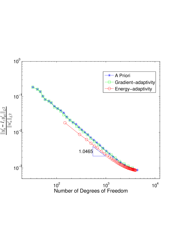
Figure 1. Relative errors in the deformation gradient (6.1) plotted against the number of degrees of freedom for three types of mesh refinements.

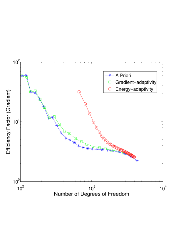
Figure 2. Efficiency factors (gradient a posteriori estimate divided by actual error) plotted against the number of degrees of freedom for three types of mesh refinements.

1. In Figure 1 we display the gradient errors for the three types of mesh generation algorithms: quasi-optimal a priori refinement, gradient-driven a posteriori refinement and energy-driven a posteriori refinement. The differences between the results produced by the three algorithms is negligable. We observe rates close to $(\#{\rm DoF})^{-1}$ for all three algorithms. The efficiency indicators (estimate divided by actual error) are displayed in Figure 2. They indicate an initial overestimation of the error, but after a sufficient accuracy is reached they enter a moderate range.

2. In Figure 3 we show the energy errors for the three types of mesh generation algorithms. Once again the differences between the three algorithms is negligable and the convergence rate is, as expected, twice the rate as compared with the gradient errors. However, the efficiency factors plotted in Figure 4 suggest that the constant prefactors in the estimators lead to a more substantial overestimation of the energy error.

We can conclude that, at least in this model problem, both a posteriori error indicators can be used to select meshes that are quasi-optimal for both the deformation gradient and for the energy. In order to obtain sharper estimates on actual errors (in particular the energy error), alternative approaches such as the goal-oriented approach [3, 24] might be preferrable.

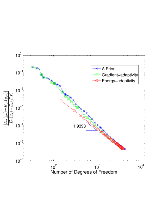
Figure 3. Relative Error of the total energy (6.1) plotted against the number of degrees of freedom for three types of mesh refinements.

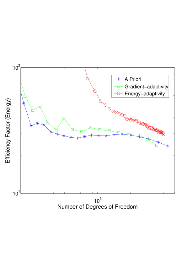
Figure 4. Efficiency Factor of the energy error estimator (energy a posteriori error estimate divided by actual energy error).

7. Conclusion

We derived a posteriori error estimators for the deformation gradient and for the energy in a 1D atomistic chain, computed by an atomistic-to-continuum coupling method. Based on these estimators we proposed two adaptive mesh refinement algorithms, which we compared to quasi-optimal a priori mesh refinement. Our numerical experiments indicate that the resulting meshes are again quasi-optimal.

While further work in the application relevant 2D/3D setting remains to be done, we conclude that adaptive mesh refinement driven by residual-based a posteriori error estimates can potentially lead to highly efficient atomistic/continuum multiscale computations of atomistic material defects.

References

- [1] Marcel Arndt and Mitchell Luskin. Goal-oriented atomistic-continuum adaptivity for the quasicontinuum approximation. Int. J. Multiscale Comput. Engrg., 5(49-50):407–415, 2007.
- [2] Marcel Arndt and Mitchell Luskin. Error estimation and atomistic-continuum adaptivity for the quasicontinuum approximation of a Frenkel-Kontorova model. Multiscale Model. Simul., 7(1):147–170, 2008.
- [3] Marcel Arndt and Mitchell Luskin. Goal-oriented adaptive mesh refinement for the quasicontinuum approximation of a Frenkel-Kontorova model. Comput. Methods Appl. Mech. Engrg., 197(49-50):4298–4306, 2008.
- [4] D Braess. Finite Elements, Theory, Fast Solvers, and Applications in Solid Mechanics, 3rd Edition. Cambridge University Press, Cambridge, 2007.
- [5] S. Brenner and R. Scott. The Mathematical Theory of Finite Element Methods, 3rd Edition. Springer, New York, 2008.
- [6] M. Dobson and M. Luskin. An analysis of the effect of ghost force oscillation on the quasicontinuum error. M2AN Math. Model. Numer. Anal., 43(3):591–604, 2009.
- [7] M. Dobson and M. Luskin. An optimal order error analysis of the one-dimensional quasicontinuum approximation. SIAM J. Numer. Anal., 47(4):2455–2475, 2009.
- [8] M. Dobson, M. Luskin, and C. Ortner. Accuracy of quasicontinuum approximations near instabilities. J. Mech. Phys. Solids, 58:1741–1757, 2010.
- [9] W. Dörfler. A convergent adaptive algorithm for poisson’s equation. SIAM J. Numer. Anal., 33:1106–1124, 1996.
- [10] X.H. Li and M. Luskin. A generalized quasi-nonlocal atomistic-to-continuum coupling method with finite range interaction. ArXiv e-prints, 1007.2336v2, 2011.
- [11] P. Lin. Theoretical and numerical analysis for the quasi-continuum approximation of a material particle model. Math. Comp., 72(242):657–675, 2003.
- [12] P. Lin. Convergence analysis of a quasi-continuum approximation for a two-dimensional material without defects. SIAM J. Numer. Anal., 45(1):313–332, 2007.
- [13] M. Luskin and C. Ortner. Atomistic-to-continuum coupling. to appear in Springer Encyclopedia on Applied and Computational Mathematics.
- [14] Ronald E Miller and E B Tadmor. A unified framework and performance benchmark of fourteen multiscale atomistic/continuum coupling methods. Modelling Simul. Mater. Sci. Eng., 17(5):053001, 2009.
- [15] P. Ming and J. Yang. Analysis of a one-dimensional nonlocal quasi-continuum method. Multiscale Model. Simul., 7(4):1838–1875, 2009.
- [16] P. Morin, R. H. Nochetto, and K. G. Siebert. Data oscillation and convergence of adaptive fem. SIAM J. Numer. Anal., 38:466–488, 2000.
- [17] M. Ortiz, R. Phillips, and E. B. Tadmor. Quasicontinuum analysis of defects in solids. Philosophical Magazine A, 73(6):1529–1563, 1996.
- [18] C. Ortner. A priori and a posteriori analysis of the quasi-nonlocal quasicontinuum method in 1d, 2009. arXiv:0911.0671, to appear in Math. Comp.
- [19] C. Ortner. The role of the patch test in 2D atomistic-to-continuum coupling methods. ArXiv e-prints, 1101.5256, 2011.
- [20] C. Ortner and M. Luskin. in preparation.
- [21] C. Ortner and A.V. Shapeev. A priori error analysis of an energy-based atomistic/continuum coupling method for pair interactions in two dimensions. arXiv:1104.0311v1.
- [22] C. Ortner and E. Süli. Analysis of a quasicontinuum method in one dimension. M2AN Math. Model. Numer. Anal., 42(1):57–91, 2008.
- [23] C. Ortner and H. WANG. A priori error estimates for energy-based quasicontinuum approximations of a periodic chain. Math. Models Methods Appl. Sci., 21(12):2491–2521, 2011.
- [24] Serge. Prudhomme, Paul. Bauman, and Tinsley Oden. Error control for molecular statics problems. Int. J. Multiscale Comput. Engrg., 4:647–662, 2007.
- [25] A. V. Shapeev. Consistent energy-based atomistic/continuum coupling for two-body potentials in three dimensions. arXiv:1108.299.
- [26] Alexander V. Shapeev. Consistent energy-based atomistic/continuum coupling for two-body potentials in one and two dimensions. Multiscale Model. Simul., 9(3):905–932, 2011.
- [27] B. Van Koten and M. Luskin. Analysis of energy-based blended quasicontinuum methods. SIAM J. Numer. Anal., 2012. arXiv:1008.2138; PLEASE UPDATE.
- [28] R. Verfurth. A Revew of A Posterori Error Estimation and Adaptive Mesh-Refinement Techniques. Wiley-Teubner, Germany, 1996.
- [29] H. Wang. A posteriori error estimates for energy-based quasicontinuum approximations of a periodic chain, 2011. arXiv:1112.5480.