The relation between frequentist confidence intervals and Bayesian credible intervals

Abstract

We investigate the relation between frequentist and Bayesian approaches. Namely, we find the “frequentist” Bayes prior $\pi_{f}(\lambda,x_{obs})=-\frac{\int_{-\infty}^{x_{obs}}\frac{\partial f(x,\lambda)}{\partial\lambda}dx}{f(x_{obs},\lambda)}$ (here $f(x,\lambda)$ is the probability density) for which the results of frequentist and Bayes approaches to the determination of confidence intervals coincide. In many cases (but not always) the “frequentist” prior which reproduces frequentist results coincides with the Jeffreys prior.

One of the standard problems in statistics [1] is an estimation of the values of unknown parameters in the probability density. There are two methods to solve this problem - the frequentist and the Bayesian.

In this paper we investigate the relation between frequentist and Bayesian approaches. Namely, we find the “frequentist” Bayes prior $\pi_{f}(\lambda,x_{obs})=-\frac{\int_{-\infty}^{x_{obs}}\frac{\partial f(x,\lambda)}{\partial\lambda}dx}{f(x_{obs},\lambda)}$ (here $f(x,\lambda)$ is the probability density) for which the results of frequentist and Bayes approaches to the determination of confidence intervals coincide. In many cases (but not always) the “frequentist” prior coincides with the Jeffreys prior. Note that in ref.[2] the relation between frequentist confidence intervals and Bayesian credible intervals has been found for probabilities densities of the special type $f(x,\lambda)=\Phi(x-\lambda)$ and $f(x,\lambda)=\frac{1}{\lambda}F(\frac{x}{\lambda})$.

As an example consider the case of random continuous observable $-\infty<x<\infty$ with the probability density $f(x,\lambda)$.

In Bayesian method [1, 3] due to Bayes theorem

$$P(A|B)=\frac{P(B|A)P(A)}{P(B)}$$ (1)

the probability density for unknown parameter $\lambda$ is determined as

$$p(\lambda|x_{obs})=\frac{f(x_{obs},\lambda)\pi(\lambda)}{\int_{-\infty}^{+\infty}f(x_{obs},\lambda^{{}^{\prime}})\pi(\lambda^{{}^{\prime}})d\lambda^{{}^{\prime}}}\,.$$ (2)

Here $x_{obs}$ is the observed value of the random variable $x$ and $\pi(\lambda)$ is the prior function. In general the prior function $\pi(\lambda)$ is not known that is the main problem of the Bayesian approach. Formula (2) reduces the statistics problem to the probability problem. The probability that parameter $\lambda$ lies in the interval $\lambda_{down}\leq\lambda\leq\lambda_{up}$ is

$$P(\lambda_{down}\leq\lambda\leq\lambda_{up})=\int_{\lambda_{down}}^{\lambda_{up}}p(\lambda|x_{obs})d\lambda=1-\alpha(\lambda_{up},\lambda_{down}|x_{obs})\,,$$ (3)

where

$$\alpha(\lambda_{up},\lambda_{down}|x_{obs})=\beta(\lambda_{up}|x_{obs})+\gamma(\lambda_{down}|x_{obs})\,,$$ (4)

$$\beta(\lambda_{up}|x_{obs})=\int^{\infty}_{\lambda_{up}}p(\lambda|x_{obs})dx\,,$$ (5)

$$\gamma(\lambda_{down}|x_{obs})=\int_{-\infty}^{\lambda_{down}}p(\lambda|x_{obs})dx=1-\beta(\lambda_{down}|x_{obs})\,,$$ (6)

The solution of the equation (3) is not unique. The most popular are the following options [1]:

1. $\lambda_{down}=-\infty$ - upper limit.

2. $\lambda_{up}=\infty$ - lower limit.

3. $\int_{-\infty}^{\lambda_{down}}p(\lambda|x_{obs})d\lambda=\int_{\lambda_{up}}^{\infty}p(\lambda|x_{obs})d\lambda=\frac{\alpha}{2}$ - symmetric interval.

4. The shortest interval - $p(\lambda|x_{obs})$ inside the interval is bigger or equal to $p(\lambda|x_{obs})$ outside the interval.

In frequentist approach the Neyman belt construction [4](see Fig. 1) is used for the determination of the confidence intervals.

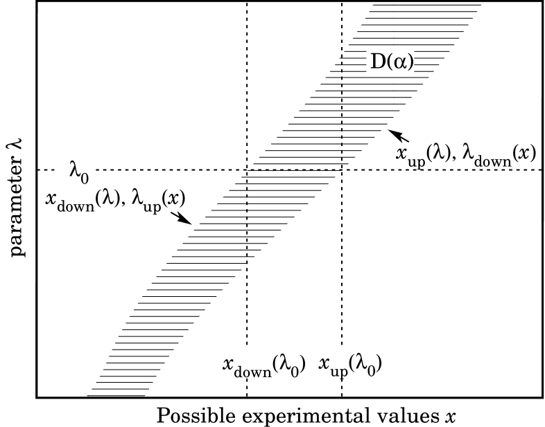
Figure 1: Neyman belt construction

Namely, we require that

$$\int^{x_{up}(\lambda)}_{x_{down}(\lambda)}f(x,\lambda)dx=1-\alpha\,,$$ (7)

or

$$\int^{\infty}_{x_{up}(\lambda)}f(x,\lambda)dx+\int_{-\infty}^{x_{down}(\lambda)}f(x,\lambda)dx=\alpha\,.$$ (8)

It should be stressed that in general case both $\int^{\infty}_{x_{up}(\lambda)}f(x,\lambda)dx$ and $\int_{-\infty}^{x_{down}(\lambda)}f(x,\lambda)dx$ can depend on $\lambda$ but their sum does not depend on $\lambda$ (see eq.(8)).

The Neyman equations for the determination of upper and lower limits $\lambda_{up}$ and $\lambda_{down}$ on parameter $\lambda$ have the form

$$\int^{x_{up}(\lambda_{up})}_{x_{obs}}f(x,\lambda_{up})dx=1-\alpha\,,$$ (9)

$$\int^{x_{obs}}_{x_{down}(\lambda_{down})}f(x,\lambda_{down})dx=1-\alpha\,$$ (10)

and they determine the confidence interval of possible values

$$\lambda_{down}\leq\lambda\leq\lambda_{up}$$ (11)

of the parameter $\lambda$ at the $(1-\alpha)$ confidence level.

In this paper we shall consider the case when $\int^{\infty}_{x_{up}(\lambda)}f(x,\lambda)dx$ does not depend on $\lambda$. For instance, the options $x_{up}(\lambda)=\infty$, $x_{down}(\lambda)=-\infty$ and $\int^{\infty}_{x_{up}(\lambda)}f(x,\lambda)dx=\int_{-\infty}^{x_{down}(\lambda)}f(x,\lambda)dx=\frac{\alpha}{2}$ correspond to the cases of upper limit on $\lambda$, lower limit on $\lambda$ and symmetric interval correspondingly. As a consequence of the eqs.(8-11) and our assumption on nondependence of $\int^{\infty}_{x_{up}(\lambda)}f(x,\lambda)dx$ on $\lambda$ we find that

$$\alpha=\int_{-\infty}^{x_{obs}}f(x,\lambda_{up})dx+\int^{\infty}_{x_{obs}}f(x,\lambda_{down})dx\,.$$ (12)

To find the relation beetween frequentist and Bayesian approaches we have to find the prior for which the formulae (4-6) and (12) coincide. Namely, we require that

$$\int_{-\infty}^{\lambda_{down}}p(\lambda|x_{obs})d\lambda+\int^{\infty}_{\lambda_{up}}p(\lambda|x_{obs})d\lambda=\int_{-\infty}^{x_{obs}}f(x,\lambda_{up})dx+\int^{\infty}_{x_{obs}}f(x,\lambda_{down})dx\,.$$ (13)

The solution of eq.(13) is

$$p(\lambda|x_{obs})=-\int_{-\infty}^{x_{obs}}\frac{\partial f(x,\lambda)}{\partial\lambda}dx\,.$$ (14)

Formulae (13,14) demonstrate the equivalence of the frequentist approach and the Bayes approach with the prior function

$$\pi_{f}(\lambda|x_{obs})=-\frac{\int_{-\infty}^{x_{obs}}\frac{\partial f(x,\lambda)}{\partial\lambda}dx}{f(x_{obs},\lambda)}\,.$$ (15)

Note that in the limit $\lambda_{down}\rightarrow-\infty$ and $\lambda_{up}\rightarrow\infty$ full probability must be equal to one, namely

$$\lim_{\lambda_{down}\rightarrow-\infty,\lambda_{up}\rightarrow\infty}\int_{-\infty}^{x_{obs}}[f(x,\lambda_{down})-f(x,\lambda_{up})]dx=1\,.$$ (16)

As a consequence of the equation (16) we find that

$$\lim_{\lambda_{down}\rightarrow-\infty}\int_{-\infty}^{x_{obs}}f(x,\lambda_{down})dx=1\,,$$ (17)

$$\lim_{\lambda_{up}\rightarrow\infty}\int^{x_{obs}}_{-\infty}f(x,\lambda_{up})dx=0\,.$$ (18)

Consider several examples. For the probability density

$$f(x,\lambda)=\Phi(x-\lambda)$$ (19)

as a consequence of the formulae (14-15) we find that

$$p_{f}(\lambda,x_{obs})=\Phi(x_{obs}-\lambda)\,,$$ (20)

$$\pi_{f}(\lambda,x_{obs})=1\,.$$ (21)

Note that for the distribution (19) the Jeffreys prior [5] $\pi(\lambda)\sim\sqrt{[\int^{\infty}_{-\infty}f(x,\lambda)(\frac{\partial ln(f(x,\lambda))}{\partial\lambda})^{2}dx]}\sim const$ does not depend on $\lambda$, i.e. for the distribution (19) the frequentist approach is equivalent to the Bayes approach with the Jeffreys prior $\pi(\lambda)=const$ [2].

Consider the case with the parameter $\lambda\geq b$. Here $b$ is some fixed number . Such situation arises when we measure signal $s$ in the presence of nonzero background $b$ and $\lambda=b+s$, $b\geq 0$, $s\geq 0$. The parameter $\lambda$ lies in the interval $b\leq\lambda<\infty$. The direct use of the formulae (12,13) leads to the inconsistency. Namely, we find that the probability

$$P(b<\lambda<\infty)=\int^{\infty}_{b}\Phi(x_{obs}-\lambda)d\lambda<1$$ (22)

that contradicts to the postulate that the full probability must be equal to 1. At the frequentist language the inequality (22) is the consequence of the fact that

$$\int^{\infty}_{x_{obs}}f(x,\lambda_{down}=b)dx\neq 0\,.$$ (23)

To obtain the correct solution we must use the language of the conditional probabilities. Really, the probability that parameter $\lambda$ lies in the interval $\lambda_{0}\leq\lambda\leq\lambda_{0}+d\lambda$ is equal to $\Phi(x_{obs}-\lambda_{0})d\lambda$. The probability that parameter $\lambda$ lies in the interval $\lambda_{0}\leq\lambda\leq\lambda_{0}+d\lambda$ provided $\lambda\geq b$ is determined by the formula of the conditional probability

$$P(\lambda_{0}\leq\lambda\leq\lambda_{0}+d\lambda|\lambda\geq b)=\frac{P(\lambda_{0}\leq\lambda\leq\lambda_{0}+d\lambda)}{P(\lambda\geq b)}=\frac{\Phi(x_{obs}-\lambda_{0})d\lambda}{\int_{b}^{\infty}\Phi(x_{obs}-\lambda)d\lambda}\,.$$ (24)

So we see that condition $\lambda\geq b$ leads to the appearance of additional factor $\int_{b}^{\infty}\Phi(x_{obs}-\lambda)d\lambda$ in the denominator of the formula (24). This factor restores the requirement that full probability $P(b_{0}\leq\lambda<\infty)=1$. For instance, the probability that signal $s$ is less than $s_{0}$ is determined by the formula

$$P(s\leq s_{0})=\frac{\int_{0}^{s_{0}}\Phi(x_{obs}-b-s)ds}{\int_{b}^{\infty}\Phi(x_{obs}-\lambda)d\lambda}$$ (25)

and it coincides with the corresponding formula of the $CL_{s}$ method [7, 8].

For the probability density

$$F(x,\lambda)=\frac{1}{\lambda}\Phi(\frac{x}{\lambda})$$ (26)

we find that

$$p_{f}(\lambda,x_{obs})=\frac{x_{obs}}{\lambda^{2}}\Phi(\frac{x_{obs}}{\lambda})\,,$$ (27)

$$\pi_{f}(\lambda,x_{obs})=\frac{x_{obs}}{\lambda}\,.$$ (28)

Again in this case the prior (28) coincides with the Jeffreys prior [2].

Consider the probability density

$$f(x,\lambda)=\theta(x)P([x],\lambda)\,,$$ (29)

where

$$P([x],\lambda)=\frac{\lambda^{[x]}}{[x]!}e^{-\lambda}$$ (30)

is the Poisson distribution and $[x]$ is an integer part of $x$ (for instance, $[2.33]=2$). Using formulae (14,15) one can find that for the probability density (29) and $x_{obs}\geq 1$

$$p_{f}(x_{obs},\lambda)=P([x_{obs}]-1,\lambda)+(x_{obs}-[x_{obs}])(-P([x_{obs}]-1,\lambda)+P([x_{obs}],\lambda))\,,$$ (31)

$$\pi_{f}(\lambda,x_{obs})=\frac{[x_{obs}]}{\lambda}+(x_{obs}-[x_{obs}])(-\frac{[x_{obs}]}{\lambda}+1)\,.$$ (32)

The Jeffreys prior for the distribution function (29) coincides with the Jeffreys prior for Poisson distribution and it is proportional to $\pi(\lambda)\sim\frac{1}{{\sqrt{\lambda}}}$. So we see that for the probability density (29) the “frequentist prior” (32) and the Jeffreys prior are different.

Consider now the case when $\int^{\infty}_{x_{up}(\lambda)}f(x,\lambda)dx$ depends on $\lambda$. Instead of $x_{up}(\lambda)$ and $x_{down}(\lambda)$ we can find another $x_{up}^{`}(\lambda)$ and $x_{down}^{`}(\lambda$ such that $x_{up}(\lambda_{up})=x_{up}^{`}(\lambda_{up})=x_{obs}$, $x_{down}(\lambda_{down})=x_{down}^{`}(\lambda_{down})=x_{obs}$ and

$$\int_{-\infty}^{x_{up}^{`}(\lambda)}f(x,\lambda)dx=\int_{\infty}^{x_{obs}}f(x,\lambda_{up})dx\,,$$ (33)

$$\int^{\infty}_{x_{down}^{`}(\lambda)}f(x,\lambda)dx=\int^{\infty}_{x_{obs}}f(x,\lambda_{down})dx\,.$$ (34)

For the confidence intervals defined by new trajectories $x_{up}^{`}(\lambda)$ and $x_{down}^{`}(\lambda)$ the Neyman equations have the form

$$\int^{x_{up}^{`}(\lambda)}_{x^{`}_{down}(\lambda)}f(x,\lambda)dx=1-\alpha^{{}^{\prime}}\,,$$ (35)

$$\alpha^{`}=\int_{-\infty}^{x_{obs}}f(x,\lambda_{up})dx+\int^{\infty}_{x_{obs}}f(x,\lambda_{down})dx\,.$$ (36)

and the equations (14,15) are valid. So we see that for the Neyman belt construction with $x_{up}^{`}(\lambda)$, $x_{down}^{`}(\lambda)$ and the integral $\int^{\infty}_{x_{down}^{`}(\lambda)}f(x,\lambda)dx$ nondependent on $\lambda$ the frequentist approach with $\alpha^{`}$ given by the exppression (36) and the Bayesian approach with prior function (14) coincide.

In conclusion let us formulate our main result. For the particular case when $\int^{\infty}_{x_{up}(\lambda)}f(x,\lambda)dx$ does not depend on $\lambda$ we have found the “frequentist” Bayes prior $\pi_{f}(\lambda,x_{obs})=-\frac{\int_{-\infty}^{x_{obs}}\frac{\partial f(x,\lambda)}{\partial\lambda}dx}{f(x_{obs},\lambda)}$ for which the results of the frequentist and the Bayes approaches to the determination of confidence intervals coincide. In many cases (but not always) the prior which reproduces frequentist results coincides with the Jeffreys prior.

This work has been supported by RFBR grant N 10-02-00468.

References

• [1] As a review, see for example:
F.James, “Statistical methods in experimental physics”, 2nd ed.,,
World Scientific, 2006.
• [2] E.T.Jaynes, “Confidence intrvals vs Bayesian intervals”, in Foundations of
Probability Theory, Statistical Inference and Statistical Theories of Science
(W.L.Harper and C.A.Hooker, eds), pp.175-257, 1976.
• [3] See, for example:
G.D‘Agostini, “Bayesian Reasoning in Data Analysis, a Critical Introduction”,
World Scientific, Hackensack, NJ, 2003.
• [4] Y.Neyman, Philos. Trans. R. Soc.London Sect. A236 333 (1937).
• [5] Harold Jeffreys, “Theory of Probability”, 3 rd ed.,
(Oxford University Press, Oxford, 1961).
• [6] G.J.Feldman and R.D.Cousins, Phys.Rev.D57 3873 (1998).
• [7] T.Junk, Nucl.Instrum.Meth. A434 435 (1999).
• [8] A.L.Read, “Modified frequentist analysis of search results(the $CL_{s}$ method)”,
CERN Yellow Report CERN-2000-005 81 (2000).