On the nature of
Phase-Type Poisson distributions
Abstract
Matrix-form Poisson probability distributions were recently introduced as one matrix generalization of Panjer distributions. We show in this paper that under the constraint that their representation is to be nonnegative, they have a physical interpretation as extensions of PH distributions, and we name this restricted family Phase-type Poisson. We use our physical interpretation to construct an EM algorithm-based estimation procedure.
AMS (2010) subject classification: 91B30; secondary 65Q30, 62P05.
Keywords: Panjer’s algorithm, generalized Panjer distributions, compound distributions, EM algorithm, minimal variance, PH-Poisson.
1 Introduction
First appeared in Panjer (1981), Panjer’s algorithm is designed to compute efficiently the density of sums of the form , where the s are i.i.d. positive random variables and is random, with a density that follows the recurrence relation
| (1) |
being such that . If the s are nonnegative integer-valued random variables with density , then the density of may be recursively computed as
| (2) |
This is a very efficient procedure, which has excellent numerical stability properties.
The distributions that satisfy (1) belong to a restricted set of families consisting of Poisson, binomial and negative binomial distributions (see Sundt and Jewell (1981)). Much effort has been spent to extend Panjer’s algorithm to other distributions for . In particular, its extension to Phase-type (PH) distributions is of great interest: since they are dense in the class of distributions on , this significantly increases the applicability of Panjer’s algorithm.
Phase-type distributions have been introduced by Neuts (1975) and (1981) and they may be defined algebraically as follows: consider a sub-stochastic matrix of order such that is nonsingular, a density vector of order , and define a sequence of row vectors with
| (3) |
The density , , for , where is a column vector of ones, is said to be of phase-type, with representation . There is a clear similarity between (1) and (3), which suggests that the recursion (2) might be adapted to provide an efficient and numerically stable algorithm to compute the density of when has a PH distribution. This is done in two recent papers, Wu and Li (2010) and Siaw et al. (2011). The former defines the generalized family as
| (4) |
where the matrices of order are recursively defined as follows:
| (5) |
The parameters are the matrices , , and the vector , which is assumed to be nonnegative and normalized, so that .
Siaw et al. (2011) define the generalized family, the difference being that the recursion (5) starts at , and the parameters are , , and , while the matrix becomes irrelevant. The PH distribution belongs to the generalized family, with , , , and .
The core of the algorithm in Wu and Li (2010) and Siaw et al. (2011) is the vector recursion
| (6) |
to replace (2), with . Ren (2010) gives an improved algorithm in case and the s themselves are of phase-type. Finally, we note that PH distributions have rational generating functions, and this is the basis for the adaptation in Eisele (2006) of Panjer’s algorithm to the case where is PH. A comparison of the complexity and numerical stability of the algorithms in Eisele (2006), Ren (2010), Wu and Li (2010) and Siaw et al. (2011) is outside the scope of the present paper.
We expect the generalized and distributions to form a very rich family since they include the PH distributions. However, as we show in the next section, the combination of two matrices in (5) makes these distributions a bit unwieldy, unless one imposes some simplifying constraint. In Section 2, we show that the series is a key quantity and that, for all practical purpose, it is necessary that the spectral radius of be strictly less than one in order for the series to converge. Before doing so, we briefly address the issue of the choice of representation, and we adopt one that is slightly different from the representation in Wu and Li (2010) and Siaw et al. (2011).
Next, we assume in Section 3 that and commute. As matrices go, this is a very strong constraint, but it considerably simplifies the determination of the generating function and of moments, and it is a property of all the examples in Wu and Li (2010) and Siaw et al. (2011). In Section 4, we focus our attention on distributions for which , , and . These distributions are interesting because they form a family totally distinct from PH distributions, yet they are amenable to a Markovian representation. For that reason, we call them Phase-type Poisson or PH-Poisson distributions. This physical interpretation opens the way in Section 5 to an estimation procedure based on the EM algorithm.
2 Matrix generating function
We are concerned with distributions defined as
| (7) |
and are matrices of order , and is a row vector of size . We use the convention that for , the matrix product in (7) is equal to the identity matrix, so that we may recursively define the s as
| (8) |
We shall write that has the representation of order .
This definition calls for a few comments. First, we assume that the recursion (7) starts with . In other words, we are not concerned in this paper with the possibility that the sequence does not conform to the general pattern for small values of . Instead, we focus our attention, to a large extent, on the matrices .
Second, our definition is slightly different from that of generalized distributions in Wu and Li (2010), where it is assumed that is a stochastic vector (, ) and that is a matrix chosen according to the circumstances. The two representations are equivalent as it suffices to define . Our reason to prefer (7) is that we do not find any advantage in requiring that should be stochastic when , and are allowed to be of mixed signs. Furthermore, our definition involves fewer parameters (the entries of ) and this savings will prove significant in Section 5 when we design an estimation procedure.
Finally, one might use left- instead of right-multiplication and define , yielding a possibly different family of distributions. Actually, we shall assume in the next section that and commute, so that there would be no difference.
We need to impose some constraints on the representations of these distributions, otherwise very little can be said in general. To begin with, let us associate a transition graph to the matrices and : the graph contains nodes, and there is an oriented arc from to if . A node is said to be useful if there exists a node such that there is a path from to in the transition graph and such that ; is said to be useless otherwise. The lemma below shows that one may require without loss of generality that representations are chosen without useless nodes.
Lemma 2.1
If the representation of order is such that there exists at least one useless node, then there exists another, equivalent, representation of order strictly less than .
Proof Assume that is a useless node; define to be the subset of nodes containing and all the nodes for which there exists a path from to . The matrices and may be written, possibly after a permutation of rows and columns, as
where and are indexed by the nodes in and and are indexed by the remaining nodes; similarly, we have
with and .
We partition in a similar manner and write . Since is useless, . It is clear that , so that is an equivalent representation, of order strictly smaller than .
The generating function may be written as , where
| (9) |
provided that the series in (9) converges. We focus our attention on the matrix generating function and we discuss its convergence properties as . A simple condition for to be finite is given in the next lemma.
Lemma 2.2
If , where denotes the spectral radius, then the series converges for .
If and , then the inequality is both necessary and sufficient.
Proof The convergence radius of the series in (9) is given by , where is any matrix norm. To simplify the notations, we define . For any consistent norm, . Furthermore, and for any , there exists a norm such that .
This implies that if , then there exist and such that for all . In addition,
for , and as . We conclude, therefore, that and , which proves the first claim.
If and are non-negative, then and ; since the last series diverges if , this completes the proof of the second claim.
Note that cannot be a necessary condition in all generality: to give one example, if there is some such that for all , then the series in (9) reduces to a finite sum, and the spectral radius of has no bearing on its convergence; such is the case if .
We turn our attention to the derivatives
| (10) |
for , assuming that they exist. In that case, the factorial moments of the distribution are given by . From the proof of Lemma 2.2, if , then is a matrix of analytic functions in the closed unit disk, and it is a sufficient condition for the derivatives to be finite at .
Lemma 2.3
The matrices are given by
| (11) |
If , then we also have
| (12) |
where
On the other hand, Lemma 1 in Wu and Li (2010) states that
If , then
for , from which (12) readily results by induction.
This lemma points to the importance of being able to determine the matrix . In some special cases, an explicit expression may be derived but in general, in the absence of any simplifying feature of the pair , there does not seem to be an alternative to the brute force calculation of the series .
3 Commutative matrix product
In this section, we assume that and commute and thereby obtain a stronger result than in Section 2. This assumption is satisfied for all examples in Wu and Li (2010), where either or is a scalar multiple of . It is also satisfied if or is a scalar matrix for some scalar , or if . The latter includes PH distributions if there exists a solution to the system of linear constraints for ; if is invertible, then an obvious solution is , .
Thus, although it is a restrictive assumption from a linear algebraic point of view, it may be reasonable in the context of stochastic modeling.
Theorem 3.1
If and commute, then , where
Furthermore, if for some integer , then and is finite, otherwise, converges if and only if .
Proof First, we observe that
| (13) |
where are Stirling’s numbers of the first kind. If and are scalars, then (13) is a straightforward consequence of the definition of Stirling’s numbers in Knuth (1968), Section 1.2.6, equation (40). To prove the extension to commuting matrices, one proceeds by induction, using
for . Next, we write
| (14) | ||||
| (15) |
since, as we show later, we may interchange the order of summation. By equations (25) and (26) in Knuth (1968), Section 1.2.9,
and (15) becomes
which proves the first claim.
If , then
Thus, it remains for us to justify the transition from (14) to (15). To that end, we show that the series is absolutely convergent if and only if . It is well-known that asymptotically as , for some integer . Furthermore, , by Theorem 1 in Wilf (1993). Therefore,
so that the series in (15) absolutely converges in if and only if , in which case its limit is . The equation (15) becomes
which converges without further constraint.
This theorem confirms the important role of the matrix with respect to the convergence of various series. A direct consequence is that if , and are three commuting matrices, then
| (16) |
so that, if and commute, we may write that
for , integer, and we may state the following property, using either (11) or (12):
Corollary 3.2
If and commute, then the th factorial moment of the distribution is given by
| (17) |
If one remembers that is a vector of which the components add-up to one, the similarity with the factorial moments of discrete PH distributions is striking (see equation (2.15) of Latouche and Ramaswami (1999)).
To conclude this section, we review the examples in Wu and Li (2010):
-
•
If for , then and .
-
•
If for , integer, as proved in Theorem 3.1.
-
•
If , then and .
We shall further examine this last case in the remainder of the paper.
4 PH-Poisson distributions
4.1 Definition and comparison to PH distributions
We restrict our attention to distributions for which , with the added constraint that , . The assumption that and are non-negative makes it easier to ascertain that is the representation of a probability distribution. In addition, as we show in Theorem 4.4, it provides us with a physical interpretation in terms of a Markovian process, which explains why we call these Phase-type Poisson distributions, or PH-Poisson for short.
Definition 4.1
A random variable has a PH-Poisson distribution with representation if
| (18) |
where is a matrix of order and is a row-vector of size such that .
Note that , unless . In the notation of Wu and Li (2010), the PH-Poisson distribution with representation belongs to the generalized () family, with , , and . The generating function is given by and the factorial moments by
| (19) |
It is easy to see that PH and PH-Poisson distributions are essentially two different families of probability distributions. Indeed, assume that is PH-Poisson with representation and is PH with representation PH(). From (18), it results that
| (20) |
asymptotically as , where is the index of , and similarly,
| (21) |
where is the index of . It is obvious that for any given there is no such that the right-hand sides of (20) and (21) coincide for all big enough, unless .
If , then there exists such that , the distribution of is concentrated on , and does have a PH representation by Theorem 2.6.5 in Latouche and Ramaswami (1999).
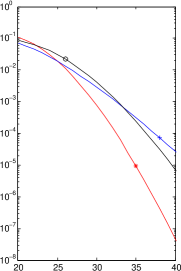
Example 4.2
Tail of the density. We see from (20) that the density of PH-Poisson distributions drops sharply to zero. We compare three different densities on Figure 1: one is a PH-Poisson distribution, the second a PH distribution and the third a Poisson distribution. We have connected the points of the densities for better visual appearance, and we plot on the right-hand side the tail of the densities in semi-logarithmic scale.
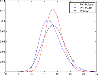
The curve marked with a “” is the density of the PH-Poisson distribution with , , , and , . The vector is given by
(it is easy to verify that .) Its mean , variance and coefficient of variation C.V. equal to are given in the first row of Table 1, as well as the spectral radius S.R. of the matrix .
| C.V. | S.R. | |||
|---|---|---|---|---|
| PH-Poisson | 18.71 | 10.35 | 0.17 | 10 |
| Phase-type | “ | 16.30 | 0.22 | 0.47 |
| Poisson | “ | 18.71 | 0.23 | 18.71 |
The curve marked with a “” is the density of the PH distributions with the same order and mean and minimal variance (see Telek (2000) for details). The curve marked with a “” is the Poisson density with parameter equal to the mean . The variance, coefficient of variation, and spectral radius of these two densities are also given in Table 1.
The plot on the right-hand side of Figure 1 clearly indicates that the PH-Poisson density decays asymptotically the fastest of the three, this is due to the combination of a relatively small spectral radius and of the factor . We also see from the plot on the left-hand side, and from Table 1, that it is the most concentrated around the mean.
Example 4.3
Small variance. We pursue here the comparison between PH-Poisson distributions and minimal variance PH distributions, showing that PH-Poisson distributions may prove to be a useful alternative to PH distributions when modeling discrete distributions with small variance.
The curve marked with a “” on Figure 2 is the density of the PH-Poisson distribution with , , , and , . The vector is given by
Its mean, variance, coefficient of variation and spectral radius are given in Table 2.
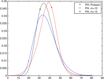
The two other curves are the density functions of PH distributions with minimal variance, with the same mean as the PH-Poisson distributions, and with different orders. The one marked with “” has the same order as the PH-Poisson distribution, the one marked with “” has order , the smallest value for which the minimal variance is smaller than that of the PH-Poisson distribution.
| C.V. | S.R. | |||
|---|---|---|---|---|
| PH-Poisson | 37.71 | 73.89 | 1.96 | 42 |
| Phase-type, | “ | 104.5 | 2.77 | 0.73 |
| Phase-type, | “ | 71.69 | 1.90 | 0.66 |
4.2 A physical interpretation
We now give a physical interpretation for PH-Poisson distributions. First, we define the Poisson process {, , …} of rate . Second, we define ; is a sub-stochastic matrix, possibly stochastic. Next, we consider a discrete PH random variable with representation , where for some arbitrary but fixed constant . In the present description, the Markov chain with transition matrix makes a transition at each event of the Poisson process and it gets absorbed at time . Finally, we count the number of transitions between transient states until the Markov chain enters its absorbing state; that is, is the number of Poisson events in the interval for and for .
Theorem 4.4
If for some arbitrary but fixed constant , then defined in (18) is the conditional probability
| (22) |
Proof Define such that
One easily verifies that and one proves by induction that
| (23) |
for . Equation (23) holds for and we assume that it holds for some . Conditioning on the epoch of the first Poisson event, we find that
Taking , we find that
so that , and
If for any scalar , then for all . This concludes the proof.
Remark 4.5
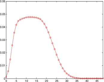
Example 4.6
This is a PH-Poisson distribution chosen to illustrate the combined effect of the conditional distribution imposed on the number of transitions among the phases. The representation is with
| (24) |
and
| (25) |
where the scaling factor is such that . Its first two moments are and , and its density is given on Figure 3.
The phase-type representation is with ,
| (26) |
and
which is the vector normalized so that .
Denote by the total number of Poisson events in . If , then , if , then . On the average, the Poisson process produces events in the interval , and the Poisson distribution has a relatively small standard deviation, so one expects to take values close to . The matrix in (26) is irreducible, albeit with a small probability of migration from one phase to another, so that the initial phase plays a significant role in the distribution of .
If the initial phase is 1, then the absorption probability is about 0.76, and it is likely that will be small; it is therefore necessary, for the condition to be fulfilled, that the Poisson process produces few events in .
On the other hand, if the initial phase is 5, then the PH Markov chain will remain in that phase for a large number of transitions, it is likely that will be large, so that is likely to be much larger than 1, and it is not expected that the condition puts much constraint on .
5 EM algorithm
In this section, we exploit the probabilistic interpretation of PH-Poisson distributions given in Section 4.2, and we develop an EM algorithm for fitting PH-Poisson distributions into data samples.
The EM algorithm is a popular iterative method in statistics for computing maximum-likelihood estimates from data that is considered incomplete. The procedure can be explained briefly as follows. Let be the set of parameters to be estimated. We denote by a random complete data sample and by its conditional density function, given the parameters . The maximum-likelihood estimator is defined as
For one reason or another, instead of observing the complete data sample , we observe an incomplete data sample . Thus, can be replaced by its sufficient statistic , where is the sufficient statistic of the unobserved data. As is unobservable, instead of maximizing we maximize its conditional expectation given the incomplete data sample and the current estimates , at each th iteration for .
The EM algorithm can thus be decomposed into two steps:
-
•
E-step—computing the conditional expectation of given the incomplete data sample and the current estimates
-
•
M-step—obtaining the next set of estimates by maximizing the expected log-likelihood determined in the E-step
When fitting a PH-Poisson distribution into a data sample, the parameters to be estimated are . Without loss of generality, we assume that in the chosen representation. By Theorem 4.4, an observation can be thought of as the number of Poisson events in the time interval , given that the transient Markov chain with the transition matrix has not been absorbed at time . This observation can be considered incomplete as it tells us neither the initial phase of the Markov chain nor how it has evolved during ; a complete observation can be represented by where is the phase of the Markov chain at the th Poisson event and for all . The conditional density of the complete observation given is
Suppose that the complete data sample contains observations, each of which is denoted by and includes an incomplete observation , for . Then, the conditional density of given is
where
is the number of complete observations in with initial phase , and
is the total number of jumps in from phase to phase . Thus, the log-likelihood function is given by
| (27) |
Maximum-likelihood estimators
To obtain closed-form expressions for the maximum-likelihood estimators is not straightforward. Applying the Karush-Kuhn-Tucker approach (see Chapter 12 in Nocedal and Wright (2000)), it can be verified that the maximization problem
| subject to | ||||
has the associated Lagrangian
where
and and denote the Lagrangian multipliers associated with the equality constraint , the inequality constraints for and , respectively. The KKT conditions, which are first-order necessary conditions for constrained optimization problems, imply that the maximum-likelihood estimators must satisfy the following constraints
| (28) | |||
| (29) | |||
| (30) |
for , where and is the column vector of size with the th component being 1 and all other components being 0.
Recall from Remark 4.5, that if is stochastic then the PH-Poisson distribution with representation is a Poisson distribution with parameter . In this case, the constraints (28)–(30) simplify considerably: the first implies that , the well-known maximum-likelihood estimator for the parameter of a Poisson distribution; the second becomes , the maximum-likelihood estimator for the initial vector of a discrete PH distribution (see Asmussen et al. (1996)); and the third reduces to
or, equivalently,
| (31) |
for . As is stochastic, summing the left-hand side of (31) over and gives us
which implies that (31) is an equality for all .
Conditional expectation
Thanks to the linear nature of in the unobserved data , the computation of the conditional expectation of at the th iteration reduces to the computation of :
| (32) |
and
| (33) |
New estimates
In the M-step, we obtain the new estimates by maximizing the log-likelihood (27) where are replaced by their conditional expectations and evaluated in the E-step. The maximization problem to be solved in this step is as follows
| subject to | ||||
We implemented the EM algorithm in MATLAB and experimented with samples simulated from different PH-Poisson distributions. Below are the results of one such experiment.
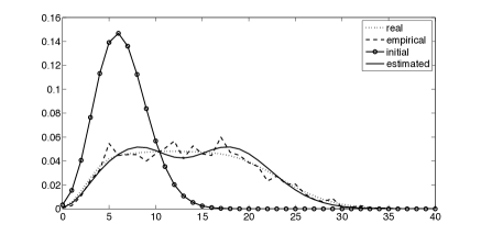
Example 5.1
We used the PH-Poisson distribution given in Example 4.6 to generate a sample with 1500 observations. The chosen initial parameters are , and
The estimated parameters obtained after 25 iterations of the EM algorithm are , , and
The Manhattan norm of the difference between the true density and the empirical data is 0.1109, between the true density and the estimated density is 0.1043, and between the empirical data and the estimated density is 0.1400. We plot four densities in Figure 4: that for the true PH-Poisson distribution, the empirical data, the initial density and the estimated density.
It is well-known that although the sequence computed with the EM algorithm always converges, it does not always converge to the maximum-likelihood estimator , but possibly to some local maximum or stationary value of . The warranty of global convergence for the EM algorithm depends on properties of the conditional density of the incomplete data given , and sometimes also on the starting point . We refer to Dempster et al. (1977) for further details on the EM algorithm, and to Wu (1983) for its convergence properties.
Our experiments were performed using the MATLAB optimization routine fmincon to solve the maximization problem in the M-step. They indicated that the results were highly sensitive to the choice of . When the starting point was chosen randomly, we observed that the EM algorithm often converged to a Poisson distribution with parameter , even if this was a rather poor fit for the given sample. Convergence to a good fit was obtained with a starting point that either shares the same structure of zeros with the true parameters and , or has a strictly positive and a diagonal matrix —a mixture of Poisson distributions.
The latter choice is obviously more practical when the structure of the true parameters is not known a priori. Empirically, a diagonal proved to be a good starting point even if the true matrix is not diagonal. Note that, unlike its counterpart for fitting discrete Phase-type distributions in Asmussen et al. (1996), the EM algorithm for fitting PH-Poisson distributions does not necessarily preserve the initial structure. This is due to the term in (27). Consequently, when starting with a diagonal the EM algorithm does not necessarily converge to a diagonal . An interesting question for future research is to explain why mixtures of Poisson distributions serve as good starting points in the EM algorithm for fitting Phase-type Poisson distributions.
Acknowledgment
All three authors thank the Ministère de la Communauté française de Belgique for funding this research through the ARC grant AUWB-08/13–ULB 5. The first and third authors also acknowledge the Australian Research Council for funding part of the work through the Discovery Grant DP110101663.
References
- [1] S. Asmussen, O. Nerman, and M. Olsson. Fitting Phase-Type distributions via the EM algorithm. Scandinavian Journal of Statistics, 23:419–441, 1996.
- [2] A. P. Dempster, N. M. Laird, and D. B. Rubin. Maximum likelihood from incomplete data via the EM algorithm (with discussion). J. Roy. Statist. Soc. Ser., 39:1–38, 1977.
- [3] K.-T. Eisele. Recursions for compound phase distributions. Insurance: Mathematics and Economics, 38:149–156, 2006.
- [4] D. E. Knuth. The Art of Computer Programming: Fundamental Algorithms, volume 1. Addison–Wesley, Reading, MA, 1968.
- [5] G. Latouche and V. Ramaswami. Introduction to Matrix Analytic Methods in Stochastic Modeling. ASA-SIAM Series on Statistics and Applied Probability. SIAM, Philadelphia PA, 1999.
- [6] M. F. Neuts. Probability distributions of phase type. In Liber Amicorum Prof. Emeritus H. Florin, pages 173–206. University of Louvain, Belgium, 1975.
- [7] M. F. Neuts. Matrix-Geometric Solutions in Stochastic Models: An Algorithmic Approach. The Johns Hopkins University Press, Baltimore, MD, 1981.
- [8] J. Nocedal and S. J. Wright. Numerical Optimization. Springer, 2000.
- [9] H. H. Panjer. Recursive evaluation of a family of compound distributions. ASTIN Bulletin, 12:22–26, 1981.
- [10] J. Ren. Recursive formulas for compound phase distributions — univariate and bivariate cases. ASTIN Bulletin, 40:615–629, 2010.
- [11] K. K. Siaw, X. Wu, D. Pitt, and Y. Wang. Matrix-form recursive evaluation of the aggregate claims distribution revisited. Annals of Actuarial Science, 5:163–179, 2011.
- [12] B. Sundt and W. S. Jewell. Further results on recursive evaluation of compound distributions. ASTIN Bulletin, 12:27–39, 1981.
- [13] M. Telek. The minimal coefficient of variation of discrete phase-type distributions. In G. Latouche and P. Taylor, editors, Advances in Algorithmic Methods for Stochastic Models – Proceedings of the 3rd International Conference on Matrix-Analytic Methods, pages 391–400. Notable Publications Inc, NJ, 2000.
- [14] H. S. Wilf. The asymptotic behavior of the Stirling numbers of the first kind. J. Comb. Theory, Ser. A, 64(2):344–349, 1993.
- [15] C. F. J. Wu. On the convergence properties of the EM algorithm. Annals of Statistics, 11:95–103, 1983.
- [16] X. Wu and S. Li. Matrix-form recursions for a family of compound distributions. ASTIN Bulletin, 40:351–368, 2010.