Abstract

We have measured the correlation function of Polyakov loops on the lattice in three dimensional $SU(3)$ gauge theory near its finite temperature phase transition. Using a new and powerful application of finite size scaling, we furthermore extend the measurements of the critical couplings to considerably larger values of the lattice sizes, both in the temperature and space directions, than was investigated earlier in this theory. With the help of these measurements we perform a detailed finite size scaling analysis, showing that for the critical exponents of the two dimensional three state Potts model the mass and the susceptibility fall on unique scaling curves. This strongly supports the expectation that the gauge theory is in the same universality class. The Nambu-Goto string model on the other hand predicts that the exponent $\nu$ has the mean field value, which is quite different from the value in the abovementioned Potts model. Using our values of the critical couplings we also determine the continuum limit of the value of the critical temperature in terms of the square root of the zero temperature string tension. This value is very near to the prediction of the Nambu-Goto string model in spite of the different critical behaviour.

1 Introduction.

Three dimensional SU(3) gauge theory has many properties in common with QCD. Lattice simulations of the theory show that the static quark potential is linear, implying confinement. They also give evidence for a mass gap and a nontrivial glueball spectrum [1]. At finite temperature there is a phase transition to a state in which the energy density is approximately described by a gluon gas. It can therefore be expected that from this model one obtains important information about the mechanism of confinement and the deconfinement transition in QCD. Furthermore, there exist analytic approximations in three dimensional $SU(N)$ gauge theory which predict the string tension and the glue ball spectrum at zero temperature [2, 3]. These results are in quite good agreement with lattice calculations [4, 5]. It is therefore important to measure the string tension at finite temperature and the value of the critical temperature, because the analytic calculations should eventually be extended to these observables.

In a series of papers [6, 7, 8, 9], we have investigated the $SU(3)$ gauge theory at finite temperature in two spatial dimensions using lattice simulations. In [6] we have shown that in the high temperature phase above approximately $1.5T_{c}$, where $T_{c}$ is the critical temperature, the theory can be dimensionally reduced to a gauge-Higgs model in two dimensions, by which one can give an excellent description of the long distance properties of the full theory. In [7] we have analysed the two dimensional gauge-Higgs model in great detail. In [8] we have investigated the thermodynamics of the three dimensional theory in the high temperature phase. We have shown, in particular, that the trace of the energy momentum tensor has a non-perturbative behaviour in a region above the phase transition, analogous to the results found in $SU(3)$ in $3+1$ dimension [10] and in full QCD [11, 12]. A detailed investigation of the thermodynamics of $SU(N)$ theories in $2+1$ dimensions with $N=2$ to $6$ has more recently been performed in Refs. [13, 14].

In [9] we studied the theory in the low temperature phase. By measuring the correlation function of Polyakov loops we obtained the finite temperature string tension. We showed that it can be very well described by the Nambu-Goto string model, as was predicted in [15, 16], but only up to a temperature $T\simeq 0.7T_{c}$, where $T_{c}$ is the critical temperature. One should remark, however, that there are analytic calculations for a general fluctuating bosonic string, which in three dimensions give universal values for the terms in the expansion in $(T/T_{c})^{2}$ up to $(T/T_{c})^{6}$ [17, 18, 19]. Not only do these terms, of course, coincide with those from the development of the formula in Nambu-Goto string model to this order, but their contribution is practically indistinguishable from the full model up to $T\simeq 0.75T_{c}$. However, such a short expansion cannot give any hint about a phase transition, while the Nambu-Goto model predicts the existence of a critical temperature $T_{c}$ at which the string tension vanishes. Moreover, it gives a value for the non perturbative ratio $T_{c}/\sqrt{\sigma_{0}}$, where $\sigma_{0}$ is the zero temperature string tension. The ratio only depends on the number of transverse dimensions. It does not depend on the group $SU(N)$. In fact, the Nambu-Goto string model gives a result for the approach of the finite temperature string tension to $T_{c}$, which corresponds to the mean field exponent $\nu=1/2$. ¿From universality arguments it is, however, expected that the transition in the $SU(3)$ gauge theory in two spatial dimensions is in the universality class of the two dimensional three state Potts model [20]. Support for this proposal has been found in lattice calculations [21].

Other comparisons of the Polyakov loop correlations in SU(3) in two spatial dimensions with the string model, in particular at lower temperatures, have been performed with a different technique in [22]. Recently, they have been extended to the group SU(6) [23]. In [13] the string model is used to estimate the behaviour of the pressure just below the transition. A good agreement with the numerical data is found.

In this article we report on an investigation of the model very near to the phase transition, a region which has not been studied up to now. First we calculate the critical couplings $\beta_{c}(N_{\tau})$, where $N_{\tau}$ is the lattice extent in the temperature direction, extending earlier calculations [21, 25] to considerably higher statistics and larger lattices. For this purpose we introduce a new and powerful method based on the work by Binder on finite size scaling [24]. Further, using results from the literature for $a\sqrt{\sigma_{0}}$, where $a$ is the lattice spacing we obtain from the continuum extrapolation a value for $T_{c}/\sqrt{\sigma_{0}}$, which can be directly compared with the prediction of the string model.

We further investigate the correlation function of the Polyakov loops below but near the critical coupling. We extract the mass and the susceptibility for a large number of spatial lattice sizes and for a range of couplings near the critical one. We consider the finite size scaling functions of these observables and find an impressive agreement with the universality class of the two dimensional three state Potts model. However, although the string and the gauge models thus have quite different critical behaviour, we find that their critical temperatures are extremely close to each other.

The plan of the paper is as follows. The definitions relative to the Polyakov loop correlations, and the set up for a critical scaling analysis of the mass gap and the susceptibility are given in Section 2. In section 3, $T_{c}/g^{2}$ is computed and the scaling properties of the susceptibility and mass gap as functions of $T/T_{c}$ exhibited. The ratio $T_{c}/\sqrt{\sigma_{0}}$ is finally computed and the gauge and string models compared. A summary and conclusions are proposed in a last section.

2 The Polyakov loop correlation function. Loop susceptibility and mass gap.

A discussion of the simulations was given in [9]. We have used the same algorithm, which was ported to GPUs (Graphical Processing Units). In this section, we first give the formulae needed for our new analysis of the physical quantities of interest, and then recall the scaling properties expected from universality near the transition.

2.1 The model and the correlation function.

The action used in the simulations is the standard Wilson lattice gauge action

$$S_{W}(U_{\mu}(\bar{x},\tau))=\beta\sum_{P}(1-\frac{1}{3}Re\operatorname{Tr}U_{P}),$$ (1)

where $U_{\mu}(\bar{x},\tau)$ denotes the group element on the link in the direction $\mu$, whose origin is located at $\bar{x}=(x_{1},x_{2})$ in space and at $\tau$ in the temperature direction. The lattice has extension $N_{S}^{2}\times N_{\tau}$. The variables $(x_{1},x_{2},\tau)$ are defined on integer values, $x_{1},x_{2}=0,1,...,N_{S}-1$ and $\tau=0,1,...,N_{\tau}-1$. The matrix $U_{P}$ is the product of link matrices around a plaquette. The constant $\beta$ is the lattice coupling constant. Note that in this article we will never use $\beta$ to denote the inverse temperature. The temperature and volume of the lattice are defined by

$$\frac{1}{T} = aN_{\tau},$$ (2)

$$V = (aN_{S})^{2}.$$ (3)

where $a$ is the lattice spacing. The coupling constant $\beta$ in the action is related to the coupling constant $g$ of the continuum action by

$$\lim_{a\rightarrow 0}(a\beta)=\frac{6}{g^{2}}.$$ (4)

In three space time dimensions, $g^{2}$ has dimension of energy, and can thus be used as the energy scale in the continuum theory.

When $N_{S}\rightarrow\infty$ at fixed $N_{\tau}$ there is a phase transitions with a critical coupling $\beta_{c}(N_{\tau})$ to a state where the $Z_{3}$ symmetry of the theory is broken. This corresponds to a finite temperature transition into a deconfined state.

To investigate the theory around the phase transition we performed numerical simulations in the neighbourhood of the transition for a large number of values of the coupling constant $\beta$ and lattice extensions $N_{S}$ and $N_{\tau}$. We study the order parameter, which in this case is the Polyakov loop. The local Polyakov loops are winding around the temperature direction:

$$L(\bar{x})=Tr\prod_{\tau=0}^{N_{\tau}-1}U_{\tau}(\bar{x},\tau).$$ (5)

We define the projected correlation function $G(z)$ between two loops at distance $z$ from each other in the $x_{1}$ direction by

$$G(z)=\frac{1}{N_{S}}\sum_{x_{2}}Re\langle L(\bar{0})L^{*}(\bar{x}=(z,x_{2}))\rangle.$$ (6)

In our earlier work [9], devoted to couplings well below $\beta_{c}(N_{\tau})$, we have represented this correlation function by

$$G(z)=b\cosh\left[m\left(\frac{N_{S}}{2}-z\right)\right].$$ (7)

The subtraction of a disconnected part from $G(z)$ would be required above $\beta_{c}(N_{\tau})$. In (7), the coefficient $b$ and the mass $m$ were fitted to the data at $z$ larger than some short distance cut off $z_{0}$. This allowed us to extract the mass gap $m$ and thereby the temperature dependent string tension

$$\frac{\sigma(T)}{T^{2}}=mN_{\tau}.$$ (8)

Fits with Eq.(7) must give stable results with respect to changes of $z_{0}$, in which case they directly provide a reliable estimate of $m$, thus of the largest correlation length $\xi=1/m$. It corresponds to the simplest situation where the correlation in $z$ decays as a pure exponential at large enough distances, and this was the case in the analysis which we reported in [9].

When we approach the phase transition, we find that this procedure does not work. In fact, making a fit with Eq. (7) the mass $m$ changes whatever $z_{0}$ we choose. Instead of trying a complicated fit in coordinate space, we prefer to transform the results to momentum space, where the analysis can be made more systematically.

The correlation function in (7) can be as well represented in momentum space by a simple pole, in the statistical mechanics called the Ornstein-Zernike (OZ) behaviour. In general, the analytic behaviour in momentum space on the negative real axis of the square of the momentum is more complicated, involving, in the continuum limit, several poles and/or cuts.

This is especially so if a continuous phase transition exists in the thermodynamical limit $N_{S}\rightarrow\infty$ at $\beta_{c}(N_{\tau})$. At the transition the correlation function is expected to decrease as a power in $z$, characterized by a critical exponent, the anomalous dimension $\eta$. As a result, close to $\beta_{c}(N_{\tau})$ and for values of $(N_{S},N_{\tau})$ accessible in practice no simple parametrization of $G(z)$ is available. Various parametrizations of its Fourier transform in the continuum limit have been proposed in the literature (for a review, see Ref. [28]). They share the property that, apart from at $\beta_{c}(N_{\tau})$, the nearest singularity remains an isolated pole in the complex plane of the momentum squared. Here, for any finite lattice, we will determine the mass gap squared as the distance to zero of the nearest pole.

We start by transforming the numerical data for the correlation function to momentum space. Given $G(z)$ on the integer values $z=0,1,...,N_{S}-1$, we define $\tilde{G}_{q}$ via

$$G(z)=\sum_{q}e^{-iqz}\tilde{G}_{q},$$ (9)

where

$$q=\frac{2\pi n}{N_{S}};\hskip 28.45274ptn=0,1,...,N_{S}-1.$$ (10)

Using the symmetries of the action, the periodic boundary conditions on the lattice and the reality of $G(z)$, it is suitable to rename $\tilde{G}_{q}$ as $\tilde{G}(p^{2})$, where to $q$ we associate

$$p=2\sin(\frac{q}{2}).$$ (11)

Given numerical data for $G(z)$ we compute the susceptibility $\chi$ of the Polyakov loop and the inverse of its Fourier transform $H(p^{2})$,

$$\tilde{G}(p^{2}) \equiv \frac{1}{N_{S}}\sum_{z=0}^{N_{S}-1}\cos(qz)G(z),$$ (12)

$$\chi = N_{S}^{2}\tilde{G}(0),$$ (13)

$$H(p^{2}) \equiv \frac{1}{\tilde{G}(p^{2})}.$$ (14)

For these measurements we restrict ourself to the disordered phase, where the subtraction of $|\langle L\rangle|^{2}$ is not necessary. On a finite lattice $\langle L\rangle=0$ also in the ordered phase in simulations which are long enough because of tunneling between the degenerate vacua.

Up to now, the functions $\tilde{G}(p^{2})$ and $H(p^{2})$ are defined only on the discrete values given in Eqs. (10, 11). We now extend these functions to arbitrary complex values of $p^{2}$, and define the mass $m$ as the first zero of $H(p^{2})$ on the negative real axis,

$$H(-m^{2})=0.$$ (15)

In the OZ approximation, we trivially get

$$H_{OZ}(p^{2}) = a_{0}+a_{1}\,p^{2},$$ (16)

$$m^{2} = \frac{a_{0}}{a_{1}}.$$ (17)

Within our assumptions, the point $p^{2}=-m^{2}$, an isolated single pole of $\tilde{G}(p^{2})$, is generically (in the thermodynamical limit) inside the circle of convergence of the series expansion of $H(p^{2})$ around zero. Because on the one hand we focus on the long range properties of the correlation, and on the other hand wish to eliminate as much as possible discretization effects, we truncate the full series of $H(p^{2})$ to a small order $n_{max}$ in $p^{2}$, and determine its coefficients from small $p^{2}$ data only. We write

$$H(p^{2})=\sum_{n=0}^{n_{\mathrm{max}}}a_{n}(p^{2})^{n},$$ (18)

and solve for $a_{n}$ the system of $n_{max}+1$ equations

$$\sum_{n=0}^{n_{\mathrm{max}}}a_{n}(p_{i}^{2})^{n}=H(p_{i}^{2})\quad;\quad i=0,1,\cdots,n_{p}$$ (19)

where $p_{i}$ are the discrete values defined by Eqs. (10, 11) and the right hand sides are measured using Eqs. (11,12,14) in $n_{p}$ points. Then $m^{2}$ is the smallest positive solution of Eq.(15). The case $n_{max}$=1 is the OZ approximation (16); the results presented in section 3 in the context of the scaling behaviour of $m$ are those obtained with $n_{max}$=2 and $n_{p}=3$. The errors quoted there are statistical errors only, estimated by a bootstrap technique applied to the whole set of configurations measured.

2.2 The setup for the critical scaling analysis

Near the phase transition one may expect that for given $N_{\tau}$ the theory is described by an effective $Z_{3}$ symmetric two-dimensional model for the Polyakov loop (5), which is in the same universality class as the two dimensional three state Potts model [20]. It should therefore have the same two independent critical exponents $\nu$ and $\eta$ as in the latter model. These are known from analytic calculations in that model to be

$$\nu = 5/6,$$ (20)

$$\eta = 4/15.$$ (21)

The universality hypothesis is supported by the results of [21]. There the critical exponents reported for $N_{\tau}=2,4$ and $6$ are, within errors, which are around $20\%$ always compatible with the above expectations.

Using the definitions (12-15), we will assume finite size scaling behaviour for $N_{S}$ large enough. Thus the mass gap and the susceptibility are represented close to the transition by

$$N_{S}\,m = f_{1}(s),$$ (22)

$$\frac{\chi}{N_{S}^{2-\eta}} \equiv N_{S}^{\eta}\,\tilde{G}(0)=f_{2}(s),$$ (23)

where

$$s=N_{S}^{1/\nu}(1-\beta/\beta_{c}(N_{\tau})),$$ (24)

and

$$f_{1}(s\to\infty) \propto s^{\nu}.$$ (25)

$$f_{2}(s\to\infty) \propto s^{-\nu(2-\eta)}.$$ (26)

Here, $\beta_{c}(N_{\tau})$, yet to be determined, denotes the critical value of the gauge coupling in the thermodynamic limit. The prefactors on the left hand sides of (22,23) are such that for $\beta$ close to $\beta_{c}(N_{\tau})$ the correlation length and the susceptibility behave in the $N_{S}\to\infty$ limit as prescribed by the critical exponents, that is

$$m \propto (1-\beta/\beta_{c}(N_{\tau}))^{\nu},$$ (27)

$$\chi \propto (1-\beta/\beta_{c}(N_{\tau}))^{-\nu(2-\eta)}.$$ (28)

In the following analysis, we assume universality to be true and use the values of $\nu$ and $\eta$ given in Eqs.(20, 21). A posteriori the fact that the data fall on unique scaling curves show that these exponents are the correct ones for the $SU(3)$ gauge theory in two spatial dimensions. For the susceptibility we make a further test of this assumption showing that the data do not fall on a universal function $f_{2}(s)$ if we assume the mean field exponent $\eta=0$.

In the next section, we use finite size scaling applied to a different quantity, more easily measurable on the lattice, in order to determine $\beta_{c}(N_{\tau})$ for $N_{\tau}=4,6,8,12$. Then the scaling assumptions of Eqs.(22 - 26) are checked with a high accuracy in the case $N_{\tau}=6$, for which a large density of data points in parameter space has been acquired. Finally an extrapolation of $\beta_{c}(N_{\tau})$ to the continuum limit $N_{\tau}\to\infty$ is performed, which allows to compare the gauge theory and the string model near their transition points.

3 Applications of finite size scaling. Critical coupling, universal scaling functions and the continuum limit compared with the string model

3.1 The critical couplings $\beta_{c}(N_{\tau})$

We recall here the properties of finite size scaling, which we need to determine the critical coupling. We determine $\beta_{c}(N_{\tau})$ from the condition that the average value $\Phi_{L}$ of a classically dimensionless functional $\Phi\{L\}$ of the effective field $L(\bar{x})$ defined by Eq.(5) does possess finite size scaling properties analogous to those of $m$ and $\chi$ in Eqs. (22,23). Generically, we set

$$N_{S}^{\phi}\,\Phi_{L} = f(s)$$ (29)

$$s = N_{S}^{1/\nu}(1-\beta/\beta_{c}(N_{\tau}))$$

$$f(s\to\infty) \propto s^{\rho},$$ (30)

where $\phi,\nu,\rho$ are critical exponents. The conditions that, in a domain including $\beta=\beta_{c}(N_{\tau})$,

i) $\Phi_{L}$ is well defined on the lattice for any $N_{S}$

ii) $\Phi_{L}$ exists in the thermodynamic limit

imply the relation

$$\rho=\nu\,\phi.$$ (31)

In this limit Eq.(29) then gives

$$\Phi_{L}\,\propto\,(1-\beta/\beta_{c}(N_{\tau}))^{\nu\phi},$$ (32)

and $\phi$ is the anomalous dimension of $\Phi$. If $\beta$ approaches $\beta_{c}(N_{\tau})$, one may expand $f(s)$ around zero and rewrite (29) as

$$N_{S}^{\phi}\,\Phi_{L}=a+bN_{S}^{1/\nu}(1-\beta/\beta_{c}(N_{\tau}))+...,$$ (33)

where $a$ and $b$ are constants. The right hand side is thus linear in $N_{S}^{1/\nu}$ at $\beta$ fixed, and $\beta_{c}(N_{\tau})$ is that value of $\beta$ for which the slope $b(1-\beta/\beta_{c}(N_{\tau}))$ vanishes. The method is, of course, particularly useful if $\phi$ and $\nu$ are known.

The order parameter $\langle L(\bar{x})\rangle$, which is classically dimensionless and has an anomalous dimension $\eta/2$ in two dimensions, does not fulfill the condition i) above since, on the lattice, it vanishes even in the broken phase, due to fluctuations between degenerate groundstates. For the same reason the susceptibility, which is quadratic in $L$ and thus has the anomalous dimension $\eta$ (see Eqs.(23,26)), is not suitable because its measurement via the definition (13) requires $\tilde{G}(0)$ to be the connected correlation (by subtracting $|\langle L\rangle|^{2}$). One could in principle use $\tilde{G}(0)$ without subtraction, but we have found that it is less stable over the transition than the variable defined below.

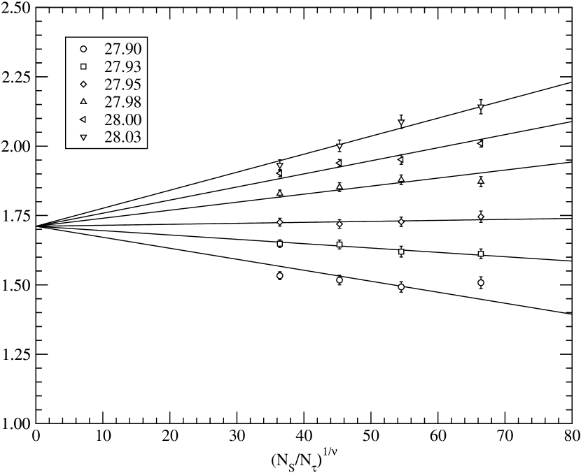
Figure 1: $N_{S}^{3\eta/2}{\cal L}_{3}$ as a function of $N_{S}^{1/\nu}$ for fixed values of $\beta$. The temporal extent is $N_{\tau}=8$. The straight lines correspond to the fits described in the text.

In fact, we consider the quantity ${\cal L}_{3}$ defined as follows

$${\cal L}=\frac{1}{N_{S}^{2}}\sum_{\bar{x}}L(\bar{x}),$$ (34)

$${\cal L}_{3}\equiv Re\langle{\cal L}^{3}\rangle.$$ (35)

This quantity is particularly interesting. $\cal L$ is the lattice average of $L(\bar{x})$, and its cube is the monomial of lowest degree that does not suffer from the same disease as $\langle L\rangle$ itself: in the ordered phase ${\cal L}^{3}$ fluctuates around the same real value whatever vacuum is chosen during the simulation. We have checked that the imaginary part of $\langle{\cal L}^{3}\rangle$ is always negligible, due to the reality of the action, and use its real part in (35) for convenience.

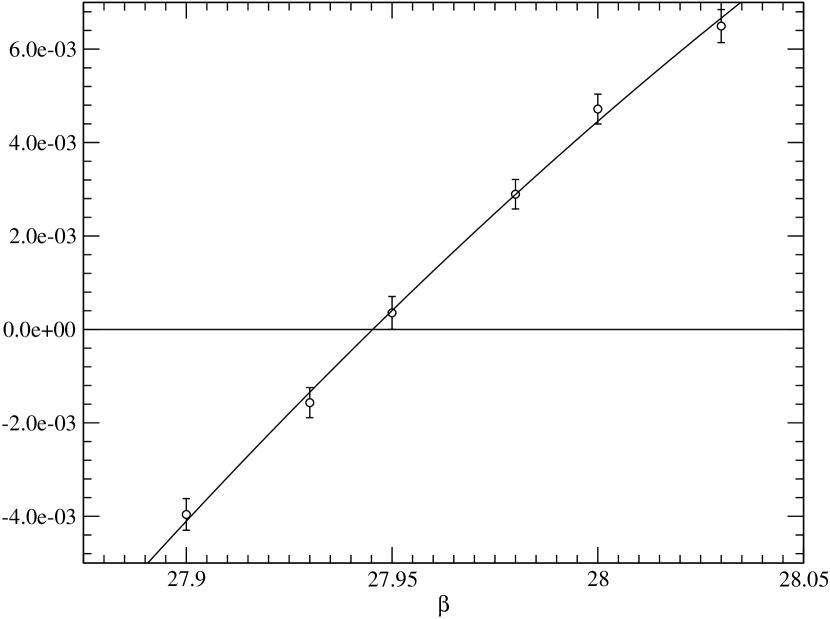
Figure 2: The slopes $\xi(\beta)$ of $N_{S}^{3\eta/2}{\cal L}_{3}$ for $N_{\tau}=8$ as a function of $\beta$. The curve corresponds to the fit described in the text.

In Fig.1 we show data obtained for ${\cal L}_{3}$ at $N_{\tau}=8$ inside a domain in $\beta$ which strongly suggests that it contains a value of $\beta$ such that ${\cal L}_{3}$ is independent of $N_{S}$. More precisely, inside the domain in $\{\beta,N_{S}\}$ shown, it appears that the data are consistent with ${\cal L}_{3}$ being linear in $N_{S}^{1/\nu}$, as expected if an expansion of the type of Eq. (33) is valid: The straight lines drawn actually result from linear fits to the data at $\beta$ fixed. They are restricted to go through the same point for vanishing argument, as demanded by Eq. (33). Similar results are obtained for the other values of $N_{\tau}$. In addition, the same ansatz (33) implies that the slopes of ${\cal L}_{3}$ in $N_{S}^{1/\nu}$ at $N_{\tau}$ fixed are proportional to $1-\beta/\beta_{c}(N_{\tau})$ near $\beta_{c}$. To take care of higher order corrections we fit the slopes, which we denote by $\xi(\beta)$, using

$$\xi(\beta)=a_{1}(\beta-\beta_{c})+a_{2}(\beta-\beta_{c})^{2},$$ (36)

where $a_{1}$ and $a_{2}$ are the parameters of the fit. These fits have very good $\chi^{2}/d.o.f.\simeq 1$. In Fig.2 we show as an example the fit for $N_{\tau}=8$, which confirms the nearly linear behaviour of the slope near $\beta_{c}$. The same is true for the other values of $N_{\tau}$ exploited. Those fits then complete the determination of $\beta_{c}(N_{\tau})$ shown in the Table below. Note that the errors are the statistical ones only. The critical coupling $\beta_{c}(4)$ has been determined in two earlier works [21] [25]. The values were $14.74(5)$ and $14.717(17)$ respectively. The method in these investigations are different from each other and from ours. Systematic errors have not been taken into account. Therefore the results are in very good agreement with ours, giving further support to our method. In Ref. [26] still another method is used to estimate the critical coupling in this theory for $N_{\tau}=4,6,8$. For $N_{\tau}=6,8$ the values are in agreement with ours within their errors, which are ten times larger. For $N_{\tau}=4$ there is a discrepancy, but this may be due to the fact that their procedure has not converged on the spatial volumes they use, which are considerably smaller than ours.

$N_{\tau}$	$\beta_{c}(N_{\tau})$
$4$	$14.7404(7)$
$6$	$21.374(3)$
$8$	$27.952(4)$
$12$	$41.075(7)$

3.2 Finite size scaling for $m$ and $\chi$

Knowing $\beta_{c}(N_{\tau})$, we are now able to test the universal scaling of the mass gap and the susceptibility. They are defined in Eqs.(15,13). Their expected finite size scaling behaviours were described in Eqs.(22 - 26). Here we illustrate the fact that, apart from a known $N_{S}$ dependent prefactor, they depend on the two parameters $\beta$ and $N_{S}$ via a function of the single variable $s$ of Eq. (24). We have measured the correlations, and thus $m$ and $\chi$ for $N_{\tau}=4$ and $6$. Here we concentrate on $N_{\tau}=6$, our conclusions for $N_{\tau}=4$ being identical. We have used values for $N_{S}$ from $48$ to $264$, and $20$ different $\beta$-values between $\beta=18$ and $21.35$, just below $\beta_{c}=21.374$.

We start with the mass because in this case only the critical exponent $\nu$ enters the analysis and thus can be probed independently. The scaling properties of the mass described by Eqs.(22,24,25) are illustrated for $N_{\tau}=6$ in Fig. 3. The quantity $mN_{S}$ is plotted versus $t^{\nu}/N_{\tau}$, where

$$t=N_{S}^{1/\nu}(1-T/T_{c}).$$ (37)

The temperature $T$ is determined through its definition (2), with the lattice spacing $a(\beta)$ obtained from a fit to the zero temperature string tension, given in our earlier paper [9], and also repeated below in Eqs. (42 - 45). It is clear from the definition in (37) that $t\simeq s$ near the transition, and thus can be used as a finite size scaling variable. The factor $1/N_{\tau}$ is inserted because according to (8), the continuum limit of the product $mN_{\tau}$ depends only on the temperature, and thus provides the leading term $(1-T/T_{c})^{\nu}$ as $N_{\tau}\to\infty$. The values of $mN_{\tau}$ collected in our earlier paper [9] for $N_{\tau}=4$ and $6$ are, in fact, found to be close one to the other.

Up to $t^{\nu}/N_{\tau}\simeq 1$ ($t\simeq 9$) , the existence of a finite size scaling law is impressively confirmed, showing a high density of points lying on one single curve. The curve is a fit to a second degree polynomial in $t$. This validates the value $\nu=5/6$ expected from universality. For $t^{\nu}/N_{\tau}\geq 1$ the data in the figure lie in the neighborhood of a straight line, corresponding to the asymptotic behaviour of Eq. (25) with the same value $\nu=5/6$.

We now probe the anomalous dimension $\eta=4/15$ appearing in the left hand side of Eq.(23). This is done in Fig. 4 by plotting $\chi/N_{S}^{(2-\eta)}$ against $mN_{S}$. This choice eliminates the explicit dependence on the critical exponent $\nu$, and therefore is a direct test of $\eta$. As we can see in the figure all the data fall on a unique scaling curve. This successfully validates $\eta=4/15$. The curve in the figure corresponds to a fit

$$\frac{\chi}{N_{S}^{2-\eta}}=\frac{b_{1}}{1+(b_{2}mN_{S})^{(2-\eta)}}$$ (38)

where $b_{1}=4.77(5)$ and $b_{2}=1.50(1)$. The form of the function has been chosen to be consistent with the expected large $N_{S}$ behavior. This behavior can be easily derived from Eqs. (22 - 26).

As already mentioned, to measure the mass gap and susceptibility above $\beta_{c}$ ($s<0$) one should subtract from $G(z)$ the disconnected contribution $|\langle L\rangle|^{2}$. On a finite lattice $\langle L\rangle$ vanishes, because of the tunneling between the degenarate vacua. In practise this happens in Monte Carlo simulations near the critical point for $N_{S}$ not too large. A popular way out is to replace $|\langle L\rangle|^{2}$ by $\langle|L|^{2}\rangle$. We will not use this procedure here. By the way, our choice to use ${\cal L}_{3}$ to identify the critical $\beta$ was dictated by the need for a control parameter which evolves smoothly across the transition.

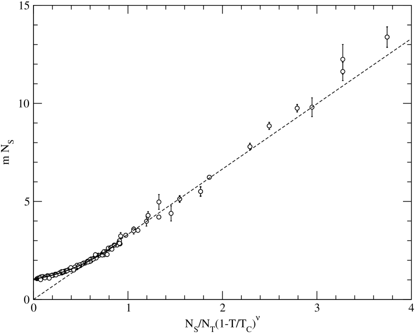
Figure 3: The scaling behaviour of the mass gap at $N_{\tau}$=6. The full line is the finite size scaling parametrization discussed in the text. The dashed line is the asymptotic behaviour given in Eqs. (24,25).

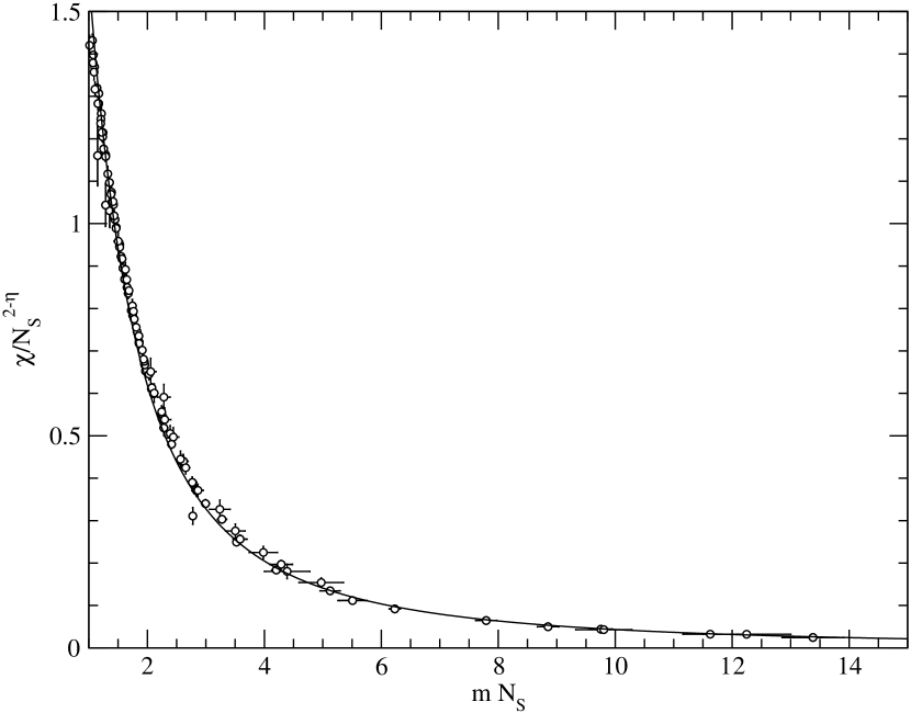
Figure 4: The scaling behaviour of the susceptibility at $N_{\tau}$=6. The curve corresponds to the fit described in the text.

The analysis described above, which has also been performed for $N_{\tau}=4$ with the same conclusions convincingly comforts the expectation that the critical behaviour of the gauge model is governed by the same exponents as the two-dimensional three states Potts model. We have not tried to determine these exponents a priori from demanding a unique scaling curve for each of the variables considered, ${\cal L}_{3},m,\chi$. But, taking the susceptibility as an example, we show a contrario in Fig. 5 that choosing the mean field exponent $\eta=0$ is far from giving a unique scaling curve.

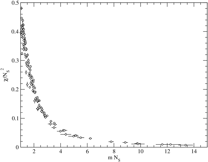
Figure 5: This figure shows the absence of a unique scaling function for the assumption of mean field exponents.

3.3 The critical temperature in the continuum compared with the string model

As shown above, for fixed $N_{\tau}$ there is a phase transition at a critical coupling $\beta_{c}(N_{\tau})$ in the thermodynamic limit $N_{S}\rightarrow\infty$. In the continuum theory there is thus a phase transition at the critical temperature $T_{c}$, given from Eqs. (2, 4) by

$$\frac{T_{c}}{g^{2}}=\lim_{N_{\tau}\rightarrow\infty}\frac{\beta_{c}(N_{\tau})}{6N_{\tau}}$$ (39)

To determine this ratio we use the data given in Table 1, and assume that the approach to the continuum limit is given by

$$\frac{\beta_{c}(N_{\tau})}{6N_{\tau}}=\frac{T_{c}}{g^{2}}(1+\frac{b}{N_{\tau}}+\frac{c}{N_{\tau}^{2}}).$$ (40)

¿From the data for the largest values of $N_{\tau}$, it is clear that the leading correction is linear in $1/N_{\tau}$. Inserting the values from Table 1 in Eq.(40), we obtain a quite good fit. We obtain

$$\frac{T_{c}}{g^{2}}=0.5446(4).$$ (41)

Another choice is to use the square root of the zero temperature string tension as energy scale. This is also what we need to compare our results with the string model. In our earlier paper [9], we used data in the literature [25] [22] to obtain the following parametrization:

$$a\sqrt{\sigma_{0}}\equiv F_{\sigma_{0}}(\beta)=\frac{h}{\beta}\frac{\beta-z}{\beta-p}$$ (42)

where

$$h = 3.325(6)$$ (43)

$$z = 2.0(2)$$ (44)

$$p = 3.7(1)$$ (45)

The form of the fitting function was choosen from the observation that $\beta F_{\sigma_{0}}(\beta)$ has a finite value when $\beta\rightarrow\infty$, and is a slowly varying function of $\beta$ in the region of the data to be fitted. A posteriori we find that the fit is very good and the value of the zero and the pole are far from the region of the data used.

On should be aware of the fact that the errors on the parameters are strongly correlated. What is important is the error on the interpolating function $F_{\sigma_{0}}(\beta)$. We found that the absolute value of the error on $1/F_{\sigma_{0}}(\beta)$ grows from 0.002 for $\beta=14$ to 0.01 for $\beta=42$. The effect of this error on $T_{c}/\sqrt{\sigma_{0}}$ was estimated using the bootstrap technique.

To obtain the continuum value of $\sqrt{\sigma_{0}}$ normalized to the scale setting parameter $g^{2}$, we form the ratio

$$\frac{\sqrt{\sigma_{0}}}{g^{2}}=\lim_{\beta\rightarrow\infty}\frac{\beta F_{\sigma_{0}}(\beta)}{6}=\frac{h}{6}=0.554(1)$$ (46)

This value is in agreement with an earlier investigation which gives a value $0.5528(8)$ for the same quantity [27], validating our parametrization of the data.

The ratio $T_{c}/\sqrt{\sigma_{0}}$ in the continuum limit is obtained from the ansatz

$$\frac{1}{N_{\tau}F_{\sigma_{0}}(\beta_{c}(N_{\tau}))}=\frac{T_{c}}{\sqrt{\sigma_{0}}}(1+\frac{c_{1}}{N_{\tau}^{2}}+\frac{c_{2}}{N_{\tau}^{4}}).$$ (47)

We find

$$\frac{T_{c}}{\sqrt{\sigma_{0}}}=0.986(1)$$ (48)

with $\chi^{2}/d.o.f=0.07$. This is lower than the value $T_{c}/\sqrt{\sigma_{0}}=0.999(4)$ in Ref. [25], where the same extrapolation formula is used, but for smaller values of $N_{\tau}=2-5$.

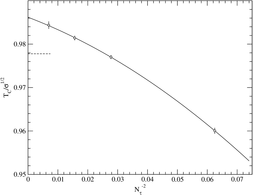
Figure 6: The quantity $T_{c}/\sqrt{\sigma_{0}}$ as a function of $1/N_{\tau}^{2}$. The full line corresponds to the fit by Eq. (47). The dashed line is the string model value in Eq. (51).

As can be seen in Fig. 6 the data show clearly that the leading correction to the continuum value in (47) has to be quadratic in $1/N_{\tau}$ as expected for a ratio between physical quantities.

In the Nambu-Goto string model, the temperature dependent string tension is predicted to be [16]

$$\sigma(T)=\sigma_{0}\sqrt{1-\frac{T^{2}}{T_{c}^{2}}}$$ (49)

where

$$T_{c}^{2}=\frac{3\sigma_{0}}{(D-2)\pi}$$ (50)

Here the constant $D$ is the number of space time dimensions of the gauge model. The prediction only depends on the number of transverse dimensions and not on the group $SU(N)$. In our case which has one transverse dimension it leads to

$$\frac{T_{c}}{\sqrt{\sigma_{0}}}=\sqrt{\frac{3}{\pi}}=0.977...$$ (51)

Furthermore Eq. (49) shows that the approach to $T_{c}$ corresponds to the mean field critical exponent $\nu=1/2$.

It is quite astonishing that the measured value (48) for $SU(3)$ is so close to the theoretical one (51), in particular as we have shown that there is a scaling region, where the mean field behaviour of the string model is not valid. In principle it would be interesting to investigate if the prediction (51) becomes better in $SU(N)$ for larger values of $N$. It has, however, been shown that for $N\geq 5$ the transition is of the first order [29, 30] as is also predicted from the universality arguments [20]. Then $\sigma(T_{c})$ has a jump, and Eq. (51) is not expected to be valid. Values of $T_{c}/\sqrt{\sigma_{0}}$ have also been obtained for $SU(2)$ and $Z_{2}$ gauge theories. In these cases the values of this ratio is quite far from the string value in Eq. (51), being $1.12(1)$ [30] and $1.237(3)$ [31, 32] respectively.

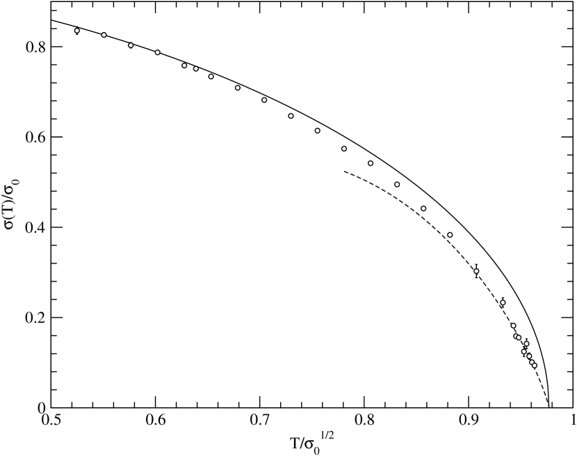
Figure 7: The quantity $\sigma(T)/\sigma_{0}$ as a function of $T/\sqrt{\sigma_{0}}$. The full line corresponds to the string model as described in the text. The dashed line shows the scaling behaviour near the transition.

Finally, we use the analysis of the correlation functions of the Polyakov loops in the region $18\leq\beta\leq 21.3$ performed in this paper to extend the comparison with the string model in [9] to the whole range below the transition. In Fig. 7 we have plotted $\sigma(T)/\sigma_{0}\equiv m/(N_{\tau}(F_{\sigma_{0}}(\beta))^{2})$ vs $T/\sqrt{\sigma_{0}}\equiv 1/(N_{\tau}F_{\sigma_{0}}(\beta))$. In the region near the transition, we only use the largest volume for each $\beta$, and further restrict to those cases where $mN_{S}>2.7$ in which case the corresponding points lie along the dashed line in Fig. 3. We compare with the prediction of the string model given in Eqs. (49,50), which does not have any free parameters. The agreement is good up to $T/\sqrt{\sigma_{0}}\approx 0.7$. Near the phase transition we compare instead with the scaling behaviour corresponding to $m=c(1-T/T_{c})^{\nu}$ , where $c$ is a free parameter. This description is satisfactory down to $T_{c}/\sqrt{\sigma_{0}}\approx 0.9$. If the data in the region in between can be described by some correction to the simple string picture as discussed in [33, 34] is still an open question. Any description of data like those in Fig. 7 must, however, be aware of the scaling region near the phase transition.

4 Conclusions

In this article we have presented results for the behaviour of three dimensional $SU(3)$ gauge theory near the finite temperature phase transition. We have introduced a new and powerful application of finite size scaling to extract the value of the critical coupling. For this purpose, we have used the third power of the Polyakov loop, which evolves smoothly over the transition. To extract $\beta_{c}$ we assume the critical exponents of the two dimensional three state Potts model, which are expected to be valid because of universality arguments [20]. Employing this method, we have determined the critical coupling on considerably larger lattices both in space and temperature direction than in earlier investigations.

That the phase transition is in the universality class of the abovementioned Potts model is strongly supported by our finite size scaling analysis of the mass gap and the susceptibility. Their values were extracted from an analysis of the correlation function of the Polyakov loop in Fourier space. We used our measured critical couplings and these correlation functions at a large set of values of the spatial extension and the coupling constant near the transition. In this region all the data for the mass gap fall within errors on a unique scaling curve, if we assume the critical exponent $\nu$ to be that of the Potts model. This test is sensitive to the exponent $\nu$ only. A further check of the universality, which is sensitive to the exponent $\eta$ was performed for the susceptibility in the disordered phase. Also in this case the data fall on a single scaling curve when we use the expected value $\eta=4/15$. This is not the case if we e.g. assume the mean field value $\eta=0$. This analysis was performed for $N_{\tau}=4$ and $6$ with consistent results.

Finally we have used our values for the critical couplings for $N_{\tau}=4,6,8$ and $12$ and the zero temperature string tension determined at these values from an interpolation formula of data in the literature to make an extrapolation to the continuum and obtain the ratio of the critical temperature to the square root of the zero temperature string tension. We have compared this ratio to the corresponding result in the Nambu-Goto string model. Although the string model predicts a temperature dependent string tension which has mean field behaviour in the scaling region, the critical temperature in this model is, in fact, very close to the lattice result. The ratio is a non perturbative and non universal observable. Thus it is a very important result, which may imply that the string model describes the spectrum and the multiplicities of the excited states of the $SU(3)$ gauge model in three space-time dimensions.

5 Acknowledgments

The simulations were done on the SHIVA computing cluster at Faculty of Physics, Astronomy and Applied Computer Science Jagiellonian University and also on ZEUS CPU and GPU cluster at Academic Computing Centre CYFRONET in Krakow and on GPU cluster at Bielefeld University. P.B. is indebted to Edwin Laerman, Olaf Kaczmarek and Marcus Fischer for the possibility to use their code and the machine and for their usual hospitality during his stay at Bielefeld. B.P. is very grateful for the kind hospitality of the Institut de Physique Théorique de Saclay, where part of this work was done.

References

- [1] M. Teper Phys. Rev. D59 (1999) 014512
- [2] D. Karabali, C. J. Kim and V. P. Nair, Phys. Lett. B434 (1998) 103 and references therein
- [3] R. G. Leigh, D. Minic and A. Yelnikov, Phys. Rev. Lett. 96 (2006) 222001; Phys. Rev. D76 (2007) 065018
- [4] B. Bringoltz and M. Teper, Phys. Lett. B645 (2007) 383
- [5] M. Teper, Phys. Rev. D59 (1999) 014512
- [6] P. Bialas, A. Morel, B. Petersson, K. Petrov and T. Reisz, Nucl. Phys. B581 (2000) 477
- [7] P. Bialas, A. Morel, B. Petersson, K. Petrov and T. Reisz, Nucl. Phys. B603 (2001) 369
- [8] P. Bialas, L. Daniel, A. Morel and B. Petersson, Nucl. Phys. B807 (2009) 547
- [9] P. Bialas, L. Daniel, A. Morel and B. Petersson, Nucl. Phys. B836 (2010) 91
- [10] G. Boyd, J. Engels, F. Karsch, E. Laermann, C. Legeland, M. Lutgemeier and B. Petersson, Nucl. Phys. B469 (1996) 419
- [11] M. Cheng et al Phys. Rev. D81 (2010) 054504
- [12] S. Borsanyi et al JHEP 0601:089 (2006), JHEP 1011:077 (2010)
- [13] M. Caselle, L. Castagnini, A. Feo, F. Gliozzi and M. Panero JHEP 06 (2011) 142
- [14] M. Caselle, L. Castagnini, A. Feo, F. Gliozzi, U. Gürsey, M. Panero and A. Schäfer, JHEP 1205 (2012) 135
- [15] R. D. Pisarski and O. Alvarez, Phys. Rev. D26 (1982) 3735
- [16] P. Olesen, Phys. Lett. B160 (1985) 408
- [17] M. Lüscher, Nucl. Phys. B180 (1981) 317
- [18] M. Lüscher and P. Weisz, JHEP 0207 (2002) 049, JHEP 0407 (2004) 049
- [19] O. Aharony and E. Karzbrun, JHEP 0906 (2009) 012
- [20] B. Svetitsky and L. G. Jaffe, Nucl. Phys. B210 (1982) 423
- [21] C. Legeland et al, Nucl. Phys. B (Proc. Suppl.) 53 (1997) 420; C. Legeland, PhD. Thesis, Bielefeld (1998).
- [22] A. Anthenodorou, B. Bringholz and M. Teper, Phys. Lett. B656 (2007) 132; PoS LAT2007 (2007) 288
- [23] A. Anthenodorou, B. Bringholz and M. Teper, [arXiv:1103.5854]
- [24] K. Binder, Z. für Physik, B43 (1981) 119.
- [25] J. Liddle and M. Teper, [arXiv:0803.2128].
- [26] N. Strodthoff, S. E. Edwards and L. von Smekal, PoS (Lattice 2010) 288.
- [27] B. Bringoltz and M. Teper, P0SLAT2006:041(2006) [arXiv: hep-lat/0610034]
- [28] A. Pelissetto and E. Vicari, Phys. Rept. 368 (2002)549.
- [29] K. Holland, JHEP 0601 (2006) 023.
- [30] J. Liddle and M. Teper, PoS LAT2005 188.
- [31] M. Caselle and M. Hasenbusch, Nucl. Phys. B470 (1996) 435.
- [32] M. Hasenbusch, Int. J. Mod. Phys. C12 (2001) 911.
- [33] M. Billo, M. Caselle, F. Gliozzi, M. Meineri and R. Pellegrini, JHEP05(2012)130.
- [34] Y. Makeenko, arXiv:1206.0922.