Order-independent constraint-based causal structure learning

Abstract

We consider constraint-based methods for causal structure learning, such as the PC-, FCI-, RFCI- and CCD- algorithms (Spirtes et al. (1993, 2000), Richardson (1996), Colombo et al. (2012), Claassen et al. (2013)). The first step of all these algorithms consists of the PC-algorithm. This algorithm is known to be order-dependent, in the sense that the output can depend on the order in which the variables are given. This order-dependence is a minor issue in low-dimensional settings. We show, however, that it can be very pronounced in high-dimensional settings, where it can lead to highly variable results. We propose several modifications of the PC-algorithm (and hence also of the other algorithms) that remove part or all of this order-dependence. All proposed modifications are consistent in high-dimensional settings under the same conditions as their original counterparts. We compare the PC-, FCI-, and RFCI-algorithms and their modifications in simulation studies and on a yeast gene expression data set. We show that our modifications yield similar performance in low-dimensional settings and improved performance in high-dimensional settings. All software is implemented in the R-package pcalg.

Keywords: directed acyclic graph, PC-algorithm, FCI-algorithm, CCD-algorithm, order-dependence, consistency, high-dimensional data

1 Introduction

Constraint-based methods for causal structure learning use conditional independence tests to obtain information about the underlying causal structure. We start by discussing several prominent examples of such algorithms, designed for different settings.

The PC-algorithm (Spirtes et al. (1993, 2000)) was designed for learning directed acyclic graphs (DAGs) under the assumption of causal sufficiency, i.e., no unmeasured common causes and no selection variables. It learns a Markov equivalence class of DAGs that can be uniquely described by a so-called completed partially directed acyclic graph (CPDAG) (see Section 2 for a precise definition). The PC-algorithm is widely used in high-dimensional settings (e.g., Kalisch et al. (2010); Nagarajan et al. (2010); Stekhoven et al. (2012); Zhang et al. (2011)), since it is computationally feasible for sparse graphs with up to thousands of variables, and open-source software is available (e.g., pcalg (Kalisch et al., 2012) and TETRAD IV (Spirtes et al., 2000)). Moreover, the PC-algorithm has been shown to be consistent for high-dimensional sparse graphs (Kalisch and Bühlmann, 2007; Harris and Drton, 2012).

The FCI- and RFCI-algorithms and their modifications (Spirtes et al. (1993, 2000, 1999); Spirtes (2001); Zhang (2008), Colombo et al. (2012), Claassen et al. (2013)) were designed for learning directed acyclic graphs when allowing for latent and selection variables. Thus, these algorithms learn a Markov equivalence class of DAGs with latent and selection variables, which can be uniquely represented by a partial ancestral graph (PAG). These algorithms first employ the PC-algorithm, and then perform additional conditional independence tests because of the latent variables.

Finally, the CCD-algorithm (Richardson, 1996) was designed for learning Markov equivalence classes of directed (not necessarily acyclic) graphs under the assumption of causal sufficiency. Again, the first step of this algorithm consists of the PC-algorithm.

Hence, all these algorithms share the PC-algorithm as a common first step. We will therefore focus our analysis on this algorithm, since any improvements to the PC-algorithm can be directly carried over to the other algorithms. When the PC-algorithm is applied to data, it is generally order-dependent, in the sense that its output depends on the order in which the variables are given. Dash and Druzdzel (1999) exploit the order-dependence to obtain candidate graphs for a score-based approach. Cano et al. (2008) resolve the order-dependence via a rather involved method based on measuring edge strengths. Spirtes et al. (2000) (Section 5.4.2.4) propose a method that removes the “weakest” edges as early as possible. Overall, however, the order-dependence of the PC-algorithm has received relatively little attention in the literature, suggesting that it seems to be regarded as a minor issue. We found, however, that the order-dependence can become very problematic for high-dimensional data, leading to highly variable results and conclusions for different variable orderings.

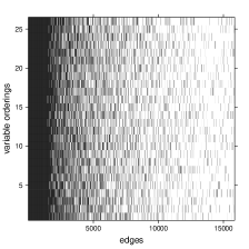
In particular, we analyzed a yeast gene expression data set (Hughes et al. (2000); see Section 6 for more detailed information) containing gene expression levels of 5361 genes for 63 wild-type yeast organisms. First, we considered estimating the skeleton of the CPDAG, that is, the undirected graph obtained by discarding all arrowheads in the CPDAG. Figure 1(a) shows the large variability in the estimated skeletons for 25 random orderings of the variables. Each estimated skeleton consists of roughly 5000 edges which can be divided into three groups: about 1500 are highly stable and occur in all orderings, about 1500 are moderately stable and occur in at least $50\%$ of the orderings, and about 2000 are unstable and occur in at most $50\%$ of the orderings. Since the FCI- and CCD-algorithms employ the PC-algorithm as a first step, their resulting skeletons for these data are also highly order-dependent.

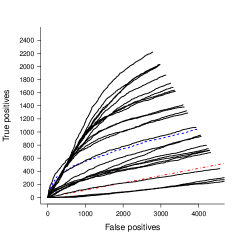
An important motivation for learning DAGs lies in their causal interpretation. We therefore also investigated the effect of different variable orderings on causal inference that is based on the PC-algorithm. In particular, we applied the IDA algorithm (Maathuis et al., 2010, 2009) to the yeast gene expression data discussed above. The IDA algorithm conceptually consists of two-steps: one first estimates the Markov equivalence class of DAGs using the PC-algorithm, and one then applies Pearl’s do-calculus (Pearl, 2000) to each DAG in the Markov equivalence class. (The algorithm uses a fast local implementation that does not require listing all DAGs in the equivalence class.) One can then obtain estimated lower bounds on the sizes of the causal effects between all pairs of genes. For each of the 25 random variable orderings, we ranked the gene pairs according to these lower bounds, and compared these rankings to a gold standard set of large causal effects computed from gene knock-out data. Figure 1(b) shows the large variability in the resulting receiver operating characteristic (ROC) curves. The ROC curve that was published in Maathuis et al. (2010) was significantly better than random guessing with $p<0.001$, and is somewhere in the middle. Some of the other curves are much better, while there are also curves that are indistinguishable from random guessing.

(a) Edges occurring in the estimated skeletons for 25 random variable orderings, as well as for the original ordering (shown as variable ordering 26). A black entry for an edge $i$ and a variable ordering $j$ means that edge $i$ occurred in the estimated skeleton for the $j$th variable ordering. The edges along the $x$-axis are ordered according to their frequency of occurrence in the estimated skeletons, from edges that occurred always to edges that occurred only once. Edges that did not occur for any of the variable orderings were omitted. For technical reasons, only every 10th edge is actually plotted.

(b) ROC curves corresponding to the 25 random orderings of the variables (solid black), where the curves are generated exactly as in Maathuis et al. (2010). The ROC curve for the original ordering of the variables (dashed blue) was published in Maathuis et al. (2010). The dashed-dotted red curve represents random guessing.

Figure 1: Analysis of the yeast gene expression data (Hughes et al., 2000) for 25 random orderings of the variables, using tuning parameter $\alpha=0.01$. The estimated graphs and resulting causal rankings are highly order-dependent.

The remainder of the paper is organized as follows. In Section 2 we discuss some background and terminology. Section 3 explains the original PC-algorithm. Section 4 introduces modifications of the PC-algorithm (and hence also of the (R)FCI- and CCD-algorithms) that remove part or all of the order-dependence. These modifications are identical to their original counterparts when perfect conditional independence information is used. When applied to data, the modified algorithms are partly or fully order-independent. Moreover, they are consistent in high-dimensional settings under the same conditions as the original algorithms. Section 5 compares all algorithms in simulations, and Section 6 compares them on the yeast gene expression data discussed above. We close with a discussion in Section 7.

2 Preliminaries

2.1 Graph terminology

A graph $\mathcal{G}=(\mathbf{V},\mathbf{E})$ consists of a vertex set $\mathbf{V}=\{X_{1},\dots,X_{p}\}$ and an edge set $\mathbf{E}$. The vertices represent random variables and the edges represent relationships between pairs of variables.

A graph containing only directed edges ($\rightarrow$) is directed, one containing only undirected edges ($-$) is undirected, and one containing directed and/or undirected edges is partially directed. The skeleton of a partially directed graph is the undirected graph that results when all directed edges are replaced by undirected edges.

All graphs we consider are simple, meaning that there is at most one edge between any pair of vertices. If an edge is present, the vertices are said to be adjacent. If all pairs of vertices in a graph are adjacent, the graph is called complete. The adjacency set of a vertex $X_{i}$ in a graph $\mathcal{G}=(\mathbf{V},\mathbf{E})$, denoted by adj$(\mathcal{G},X_{i})$, is the set of all vertices in $\mathbf{V}$ that are adjacent to $X_{i}$ in $\mathcal{G}$. A vertex $X_{j}$ in adj$(\mathcal{G},X_{i})$ is called a parent of $X_{i}$ if $X_{j}\rightarrow X_{i}$. The corresponding set of parents is denoted by pa$(\mathcal{G},X_{i})$.

A path is a sequence of distinct adjacent vertices. A directed path is a path along directed edges that follows the direction of the arrowheads. A directed cycle is formed by a directed path from $X_{i}$ to $X_{j}$ together with the edge $X_{j}\rightarrow X_{i}$. A (partially) directed graph is called a (partially) directed acyclic graph if it does not contain directed cycles.

A triple $(X_{i},X_{j},X_{k})$ in a graph $\mathcal{G}$ is unshielded if $X_{i}$ and $X_{j}$ as well as $X_{j}$ and $X_{k}$ are adjacent, but $X_{i}$ and $X_{k}$ are not adjacent in $\mathcal{G}$. A v-structure $(X_{i},X_{j},X_{k})$ is an unshielded triple in a graph $\mathcal{G}$ where the edges are oriented as $X_{i}\rightarrow X_{j}\leftarrow X_{k}$.

2.2 Probabilistic and causal interpretation of DAGs

We use the notation $X_{i}\perp\perp X_{j}|\mathbf{S}$ to indicate that $X_{i}$ is independent of $X_{j}$ given $\mathbf{S}$, where $\mathbf{S}$ is a set of variables not containing $X_{i}$ and $X_{j}$ (Dawid, 1980). If $\mathbf{S}$ is the empty set, we simply write $X_{i}\perp\perp X_{j}$. If $X_{i}\perp\perp X_{j}|\mathbf{S}$, we refer to $\mathbf{S}$ as a separating set for $(X_{i},X_{j})$. A separating set $\mathbf{S}$ for $(X_{i},X_{j})$ is called minimal if there is no proper subset $\mathbf{S^{\prime}}$ of $\mathbf{S}$ such that $X_{i}\perp\perp X_{j}|\mathbf{S^{\prime}}$.

A distribution $Q$ is said to factorize according to a DAG $\mathcal{G}=(\mathbf{V},\mathbf{E})$ if the joint density of $\mathbf{V}=(X_{1},\dots,X_{p})$ can be written as the product of the conditional densities of each variable given its parents in $\mathcal{G}$: $q(X_{1},\dots,X_{p})=\prod_{i=1}^{p}q(X_{i}|\text{pa}(\mathcal{G},X_{i}))$.

A DAG entails conditional independence relationships via a graphical criterion called d-separation (Pearl, 2000). If two vertices $X_{i}$ and $X_{j}$ are not adjacent in a DAG $\mathcal{G}$, then they are d-separated in $\mathcal{G}$ by a subset $\mathbf{S}$ of the remaining vertices. If $X_{i}$ and $X_{j}$ are d-separated by $\mathbf{S}$, then $X_{i}\perp\perp X_{j}|\mathbf{S}$ in any distribution $Q$ that factorizes according to $\mathcal{G}$. A distribution $Q$ is said to be faithful to a DAG $\mathcal{G}$ if the reverse implication also holds, that is, if the conditional independence relationships in $Q$ are exactly the same as those that can be inferred from $\mathcal{G}$ using d-separation.

Several DAGs can describe exactly the same conditional independence information. Such DAGs are called Markov equivalent and form a Markov equivalence class. Markov equivalent DAGs have the same skeleton and the same v-structures, and a Markov equivalence class can be described uniquely by a completed partially directed acyclic graph (CPDAG) (Andersson et al., 1997; Chickering, 2002). A CPDAG is a partially directed acyclic graph with the following properties: every directed edge exists in every DAG in the Markov equivalence class, and for every undirected edge $X_{i}-X_{j}$ there exists a DAG with $X_{i}\rightarrow X_{j}$ and a DAG with $X_{i}\leftarrow X_{j}$ in the Markov equivalence class. A CPDAG $\mathcal{C}$ is said to represent a DAG $\mathcal{G}$ if $\mathcal{G}$ belongs to the Markov equivalence class described by $\mathcal{C}$.

A DAG can be interpreted causally in the following way (Pearl, 2000, 2009; Spirtes et al., 2000): $X_{1}$ is a direct cause of $X_{2}$ only if $X_{1}\rightarrow X_{2}$, and $X_{1}$ is a possibly indirect cause of $X_{2}$ only if there is a directed path from $X_{1}$ to $X_{2}$.

3 The PC-algorithm

We now describe the PC-algorithm in detail. In Section 3.1, we discuss the algorithm under the assumption that we have perfect conditional independence information between all variables in $\mathbf{V}$. We refer to this as the oracle version. In Section 3.2 we discuss the more realistic situation where conditional independence relationships have to be estimated from data. We refer to this as the sample version.

3.1 Oracle version

A sketch of the PC-algorithm is given in Algorithm 3.1. We see that the algorithm consists of three steps. Step 1 finds the skeleton and separation sets, while Steps 2 and 3 determine the orientations of the edges.

Algorithm 3.1 The PC-algorithm (oracle version)

0:  Conditional independence information among all variables in $\mathbf{V}$, and an ordering $\text{order}(\mathbf{V})$ on the variables

1:  Find the skeleton $\mathcal{C}$ and separation sets using Algorithm 3.2;

2:  Orient unshielded triples in the skeleton $\mathcal{C}$ based on the separation sets;

3:  In $\mathcal{C}$ orient as many of the remaining undirected edges as possible by repeated application of rules R1-R3 (see text);

4:  return  Output graph $(\mathcal{C})$ and separation sets (sepset).

Algorithm 3.2 Step 1 of the PC-algorithm (oracle version)

0:  Conditional independence information among all variables in $\mathbf{V}$, and an ordering order$(\mathbf{V})$ on the variables

1:  Form the complete undirected graph $\mathcal{C}$ on the vertex set $\mathbf{V}$

2:  Let $\ell=-1$;

3:  repeat

4:     Let $\ell=\ell+1$;

5:     repeat

6:        Select a (new) ordered pair of vertices $(X_{i},X_{j})$ that are adjacent in $\mathcal{C}$ and satisfy $|\text{adj}(\mathcal{C},X_{i})\setminus\{X_{j}\}|\geq\ell$, using order$(\mathbf{V})$;

7:        repeat

8:           Choose a (new) set $\mathbf{S}\subseteq\text{adj}(\mathcal{C},X_{i})\setminus\{X_{j}\}$ with $|\mathbf{S}|=\ell$, using order$(\mathbf{V})$;

9:           if $X_{i}$ and $X_{j}$ are conditionally independent given $\mathbf{S}$ then

10:              Delete edge $X_{i}-X_{j}$ from $\mathcal{C}$;

11:              Let $\text{sepset}(X_{i},X_{j})=\text{sepset}(X_{j},X_{i})=\mathbf{S}$;

12:           end if

13:        until $X_{i}$ and $X_{j}$ are no longer adjacent in $\mathcal{C}$ or all $\mathbf{S}\subseteq\text{adj}(\mathcal{C},X_{i})\setminus\{X_{j}\}$ with $|\mathbf{S}|=\ell$ have been considered

14:     until all ordered pairs of adjacent vertices $(X_{i},X_{j})$ in $\mathcal{C}$ with $|\text{adj}(\mathcal{C},X_{i})\setminus\{X_{j}\}|\geq\ell$ have been considered

15:  until all pairs of adjacent vertices $(X_{i},X_{j})$ in $\mathcal{C}$ satisfy $|\text{adj}(\mathcal{C},X_{i})\setminus\{X_{j}\}|\leq\ell$

16:  return  $\mathcal{C}$, sepset.

Step 1 is given in pseudo-code in Algorithm 3.2. We start with a complete undirected graph $\mathcal{C}$. This graph is subsequently thinned out in the loop on lines 3-15 in Algorithm 3.2, where an edge $X_{i}-X_{j}$ is deleted if $X_{i}\perp\perp X_{j}|\mathbf{S}$ for some subset $\mathbf{S}$ of the remaining variables. These conditional independence queries are organized in a way that makes the algorithm computationally efficient for high-dimensional sparse graphs.

First, when $\ell=0$, all pairs of vertices are tested for marginal independence. If $X_{i}\perp\perp X_{j}$, then the edge $X_{i}-X_{j}$ is deleted and the empty set is saved as separation set in $\text{sepset}(X_{i},X_{j})$ and $\text{sepset}(X_{j},X_{i})$. After all pairs of vertices have been considered (and many edges might have been deleted), the algorithm proceeds to the next step with $\ell=1$.

When $\ell=1$, the algorithm chooses an ordered pair of vertices $(X_{i},X_{j})$ still adjacent in $\mathcal{C}$, and checks $X_{i}\perp\perp X_{j}|\mathbf{S}$ for subsets $\mathbf{S}$ of size $\ell=1$ of $\text{adj}(\mathcal{C},X_{i})\setminus\{X_{j}\}$. If such a conditional independence is found, the edge $X_{i}-X_{j}$ is removed, and the corresponding conditioning set $\mathbf{S}$ is saved in $\text{sepset}(X_{i},X_{j})$ and $\text{sepset}(X_{j},X_{i})$. If all ordered pairs of adjacent vertices have been considered for conditional independence given all subsets of size $\ell$ of their adjacency sets, the algorithm again increases $\ell$ by one. This process continues until all adjacency sets in the current graph are smaller than $\ell$. At this point the skeleton and the separation sets have been determined.

Step 2 determines the v-structures. In particular, it considers all unshielded triples in $\mathcal{C}$, and orients an unshielded triple $(X_{i},X_{j},X_{k})$ as a v-structure if and only if $X_{j}\notin\text{sepset}(X_{i},X_{k})$.

Finally, Step 3 orients as many of the remaining undirected edges as possible by repeated application of the following three rules:

1. orient $X_{j}-X_{k}$ into $X_{j}\rightarrow X_{k}$ whenever there is a directed edge $X_{i}\rightarrow X_{j}$ such that $X_{i}$ and $X_{k}$ are not adjacent (otherwise a new v-structure is created);

2. orient $X_{i}-X_{j}$ into $X_{i}\rightarrow X_{j}$ whenever there is a chain $X_{i}\rightarrow X_{k}\rightarrow X_{j}$ (otherwise a directed cycle is created);

3. orient $X_{i}-X_{j}$ into $X_{i}\rightarrow X_{j}$ whenever there are two chains $X_{i}-X_{k}\rightarrow X_{j}$ and $X_{i}-X_{l}\rightarrow X_{j}$ such that $X_{k}$ and $X_{l}$ are not adjacent (otherwise a new v-structure or a directed cycle is created).

The PC-algorithm was shown to be sound and complete.

Theorem 1

(Theorem 5.1 on p.410 of Spirtes et al. (2000)) Let the distribution of $\mathbf{V}$ be faithful to a DAG $\mathcal{G}=(\mathbf{V},\mathbf{E})$, and assume that we are given perfect conditional independence information about all pairs of variables $(X_{i},X_{j})$ in $\mathbf{V}$ given subsets $\mathbf{S}\subseteq\mathbf{V}\setminus\{X_{i},X_{j}\}$. Then the output of the PC-algorithm is the CPDAG that represents $\mathcal{G}$.

We briefly discuss the main ingredients of the proof, as these will be useful for understanding our modifications in Section 4. The faithfulness assumption implies that conditional independence in the distribution of $\mathbf{V}$ is equivalent to d-separation in the graph $\mathcal{G}$. The skeleton of $\mathcal{G}$ can then be determined as follows: $X_{i}$ and $X_{j}$ are adjacent in $\mathcal{G}$ if and only if they are conditionally dependent given any subset $\mathbf{S}$ of the remaining nodes. Naively, one could therefore check all these conditional dependencies, which is known as the SGS algorithm (Spirtes et al., 2000). The PC-algorithm obtains the same result with fewer tests, by using the following fact about DAGs: two variables $X_{i}$ and $X_{j}$ in a DAG $\mathcal{G}$ are d-separated by some subset $\mathbf{S}$ of the remaining variables if and only if they are d-separated by $\text{pa}(\mathcal{G},X_{i})$ or $\text{pa}(\mathcal{G},X_{j})$. The PC-algorithm is guaranteed to check these conditional independencies: at all stages of the algorithm, the graph $\mathcal{C}$ is a supergraph of the true CPDAG, and the algorithm checks conditional dependencies given all subsets of the adjacency sets, which obviously include the parent sets.

The v-structures are determined based on Lemmas 5.1.2 and 5.1.3 of Spirtes et al. (2000). The soundness and completeness of the orientation rules in Step 3 was shown in Meek (1995) and Andersson et al. (1997).

3.2 Sample version

In applications, we of course do not have perfect conditional independence information. Instead, we assume that we have an i.i.d. sample of size $n$ of $\mathbf{V}=(X_{1},\dots,X_{p})$. A sample version of the PC-algorithm can then be obtained by replacing all steps where conditional independence decisions were taken by statistical tests for conditional independence at some pre-specified level $\alpha$. For example, if the distribution of $\mathbf{V}$ is multivariate Gaussian, one can test for zero partial correlation, see, e.g., Kalisch and Bühlmann (2007). We note that the significance level $\alpha$ is used for many tests, and plays the role of a tuning parameter, where smaller values of $\alpha$ tend to lead to sparser graphs.

3.3 Order-dependence in the sample version

Let order($\mathbf{V}$) denote an ordering on the variables in $\mathbf{V}$. We now consider the role of order($\mathbf{V}$) in every step of the algorithm. Throughout, we assume that all tasks are performed according to the lexicographical ordering of order$(\mathbf{V})$, which is the standard implementation in pcalg (Kalisch et al., 2012) and TETRAD IV (Spirtes et al., 2000), and is called “PC-1” in Spirtes et al. (2000) (Section 5.4.2.4).

In Step 1, order($\mathbf{V}$) affects the estimation of the skeleton and the separating sets. In particular, at each level of $\ell$, order($\mathbf{V}$) determines the order in which pairs of adjacent vertices and subsets $\mathbf{S}$ of their adjacency sets are considered (see lines 6 and 8 in Algorithm 3.2). The skeleton $\mathcal{C}$ is updated after each edge removal. Hence, the adjacency sets typically change within one level of $\ell$, and this affects which other conditional independencies are checked, since the algorithm only conditions on subsets of the adjacency sets. In the oracle version, we have perfect conditional independence information, and all orderings on the variables lead to the same output. In the sample version, however, we typically make mistakes in keeping or removing edges. In such cases, the resulting changes in the adjacency sets can lead to different skeletons, as illustrated in Example 1.

Moreover, different variable orderings can lead to different separating sets in Step 1. In the oracle version, this is not important, because any valid separating set leads to the correct v-structure decision in Step 2. In the sample version, however, different separating sets in Step 1 of the algorithm may yield different decisions about v-structures in Step 2. This is illustrated in Example 2.

Finally, we consider the role of order($\mathbf{V}$) on the orientation rules in Steps 2 and 3 of the sample version of the PC-algorithm. Example 3 illustrates that different variable orderings can lead to different orientations, even if the skeleton and separating sets are order-independent.

Example 1

(Order-dependent skeleton in the sample PC-algorithm.) Suppose that the distribution of $\mathbf{V}=\{X_{1},X_{2},X_{3},X_{4},X_{5}\}$ is faithful to the DAG in Figure 2(a). This DAG encodes the following conditional independencies with minimal separating sets: $X_{1}\perp\perp X_{2}$ and $X_{2}\perp\perp X_{4}|\{X_{1},X_{3}\}$ .

Suppose that we have an i.i.d. sample of $(X_{1},X_{2},X_{3},X_{4},X_{5})$, and that the following conditional independencies with minimal separating sets are judged to hold at some level $\alpha$: $X_{1}\perp\perp X_{2}$, $X_{2}\perp\perp X_{4}|\{X_{1},X_{3}\}$, and $X_{3}\perp\perp X_{4}|\{X_{1},X_{5}\}$. Thus, the first two are correct, while the third is false.

We now apply the PC-algorithm with two different orderings: $\text{order}_{1}(\mathbf{V})=(X_{1},X_{4},X_{2},\linebreak X_{3},X_{5})$ and $\text{order}_{2}(\mathbf{V})=(X_{1},X_{3},X_{4},X_{2},X_{5})$. The resulting skeletons are shown in Figures 2(b) and 2(c), respectively. We see that the skeletons are different, and that both are incorrect as the edge $X_{3}-X_{4}$ is missing. The skeleton for $\text{order}_{2}(\mathbf{V})$ contains an additional error, as there is an additional edge $X_{2}-X_{4}$.

We now go through Algorithm 3.2 to see what happened. We start with a complete undirected graph on $\mathbf{V}$. When $\ell=0$, variables are tested for marginal independence, and the algorithm correctly removes the edge between $X_{1}$ and $X_{2}$. No other conditional independencies are found when $\ell=0$ or $\ell=1$. When $\ell=2$, there are two pairs of vertices that are thought to be conditionally independent given a subset of size 2, namely the pairs $(X_{2},X_{4})$ and $(X_{3},X_{4})$.

In $\text{order}_{1}(\mathbf{V})$, the pair $(X_{4},X_{2})$ is considered first. The corresponding edge is removed, as $X_{4}\perp\perp X_{2}|\{X_{1},X_{3}\}$ and $\{X_{1},X_{3}\}$ is a subset of $\text{adj}(\mathcal{C},X_{4})=\{X_{1},X_{2},X_{3},X_{5}\}$. Next, the pair $(X_{4},X_{3})$ is considered and the corresponding edges is erroneously removed, because of the wrong decision that $X_{4}\perp\perp X_{3}|\{X_{1},X_{5}\}$ and the fact that $\{X_{1},X_{5}\}$ is a subset of $\text{adj}(\mathcal{C},X_{4})=\{X_{1},X_{3},X_{5}\}$.

In $\text{order}_{2}(\mathbf{V})$, the pair $(X_{3},X_{4})$ is considered first, and the corresponding edge is erroneously removed. Next, the algorithm considers the pair $(X_{4},X_{2})$. The corresponding separating set $\{X_{1},X_{3}\}$ is not a subset of $\text{adj}(\mathcal{C},X_{4})=\{X_{1},X_{2},X_{5}\}$, so that the edge $X_{2}-X_{4}$ remains. Next, the algorithm considers the pair $(X_{2},X_{4})$. Again, the separating set $\{X_{1},X_{3}\}$ is not a subset of $\text{adj}(\mathcal{C},X_{2})=\{X_{3},X_{4},X_{5}\}$, so that the edge $X_{2}-X_{4}$ again remains. In other words, since $(X_{3},X_{4})$ was considered first in $\text{order}_{2}(\mathbf{V})$, the adjacency set of $X_{4}$ was affected and no longer contained $X_{3}$, so that the algorithm “forgot” to check the conditional independence $X_{2}\perp\perp X_{4}|\{X_{1},X_{3}\}$.

(a) True DAG.

(b) Skeleton returned by the oracle version of Algorithm 3.2 with any ordering, and by the sample version of Algorithm 3.2 with $\text{order}_{1}(\mathbf{V})$.

(c) Skeleton returned by the sample version of Algorithm 3.2 with $\text{order}_{2}(\mathbf{V})$.

Figure 2: Graphs corresponding to Examples 1 and 4.

Example 2

(Order-dependent separating sets and v-structures in the sample PC-algorithm.) Suppose that the distribution of $\mathbf{V}=\{X_{1},X_{2},X_{3},X_{4},X_{5}\}$ is faithful to the DAG in Figure 3(a). This DAG encodes the following conditional independencies with minimal separating sets: $X_{1}\perp\perp X_{3}|\{X_{2}\}$, $X_{1}\perp\perp X_{4}|\{X_{2}\}$, $X_{1}\perp\perp X_{4}|\{X_{3}\}$, $X_{2}\perp\perp X_{4}|\{X_{3}\}$, $X_{2}\perp\perp X_{5}|\{X_{1},X_{3}\}$, $X_{2}\perp\perp X_{5}|\{X_{1},X_{4}\}$, $X_{3}\perp\perp X_{5}|\{X_{1},X_{4}\}$ and $X_{3}\perp\perp X_{5}|\{X_{2},X_{4}\}$.

We consider the oracle PC-algorithm with two different orderings on the variables: $\text{order}_{3}(\mathbf{V})=(X_{1},X_{4},X_{2},X_{3},X_{5})$ and $\text{order}_{4}(\mathbf{V})=(X_{1},X_{4},X_{3},X_{2},X_{5})$. For $\text{order}_{3}(\mathbf{V})$, we obtain sepset$(X_{1},X_{4})=\{X_{2}\}$, while for $\text{order}_{4}(\mathbf{V})$ we get sepset$(X_{1},X_{4})=\{X_{3}\}$. Thus, the separating sets are order-dependent. However, we obtain the same v-structure $X_{1}\to X_{5}\leftarrow X_{4}$ for both orderings, since $X_{5}$ is not in the sepset$(X_{1},X_{4})$, regardless of the ordering. In fact, this holds in general, since in the oracle version of the PC-algorithm, a vertex is either in all possible separating sets or in none of them (cf. (Spirtes et al., 2000, Lemma 5.1.3)).

Now suppose that we have an i.i.d. sample of $(X_{1},X_{2},X_{3},X_{4},X_{5})$. Suppose that at some level $\alpha$, all true conditional independencies are judged to hold, and $X_{1}\perp\perp X_{3}|\{X_{4}\}$ is thought to hold by mistake. We again consider two different orderings: $\text{order}_{5}(\mathbf{V})=(X_{1},X_{3},X_{4},X_{2},X_{5})$ and $\text{order}_{6}(\mathbf{V})=(X_{3},X_{1},X_{2},X_{4},X_{5})$. With $\text{order}_{5}(\mathbf{V})$ we obtain the incorrect $\text{sepset}(X_{1},X_{3})=\{X_{4}\}$. This also leads to an incorrect v-structure $X_{1}\to X_{2}\leftarrow X_{3}$ in Step 2 of the algorithm. With $\text{order}_{6}(\mathbf{V})$, we obtain the correct $\text{sepset}(X_{1},X_{3})=\{X_{2}\}$, and hence correctly find that $X_{1}-X_{2}-X_{3}$ is not a v-structure in Step 2. This illustrates that order-dependent separating sets in Step 1 of the sample version of the PC-algorithm can lead to order-dependent v-structures in Step 2 of the algorithm.

(a) True DAG.

(b) Output of the oracle PC-algorithm with any ordering, and of the sample PC-algorithm with $\text{order}_{6}(\mathbf{V})$.

(c) Output of the sample PC-algorithm with $\text{order}_{5}(\mathbf{V})$.

Figure 3: Graphs corresponding to Examples 2 and 5.

Example 3

(Order-dependent orientation rules in Steps 2 and 3 of the sample PC-algorithm.) Consider the graph in Figure 4(a) with two unshielded triples $(X_{1},X_{2},X_{3})$ and $(X_{2},X_{3},X_{4})$, and assume this is the skeleton after Step 1 of the sample version of the PC-algorithm. Moreover, assume that we found $\text{sepset}(X_{1},X_{3})=\text{sepset}(X_{2},X_{4})=\text{sepset}(X_{1},X_{4})=\emptyset$. Then in Step 2 of the algorithm, we obtain two v-structures $X_{1}\to X_{2}\leftarrow X_{3}$ and $X_{2}\to X_{3}\leftarrow X_{4}$. Of course this means that at least one of the statistical tests is wrong, but this can happen in the sample version. We now have conflicting information about the orientation of the edge $X_{2}-X_{3}$. In the current implementation of pcalg, where conflicting edges are simply overwritten, this means that the orientation of $X_{2}-X_{3}$ is determined by the v-structure that is last considered. Thus, we obtain $X_{1}\to X_{2}\to X_{3}\leftarrow X_{4}$ if $(X_{2},X_{3},X_{4})$ is considered last, while we get $X_{1}\to X_{2}\leftarrow X_{3}\leftarrow X_{4}$ if $(X_{1},X_{2},X_{3})$ is considered last.

Next, consider the graph in Figure 4(b), and assume that this is the output of the sample version of the PC-algorithm after Step 2. Thus, we have two v-structures, namely $X_{1}\rightarrow X_{2}\leftarrow X_{3}$ and $X_{4}\rightarrow X_{5}\leftarrow X_{6}$, and four unshielded triples, namely $(X_{1},X_{2},X_{5})$, $(X_{3},X_{2},X_{5})$, $(X_{4},X_{5},X_{2})$, and $(X_{6},X_{5},X_{2})$. Thus, we then apply the orientation rules in Step 3 of the algorithm, starting with rule R1. If one of the two unshielded triples $(X_{1},X_{2},X_{5})$ or $(X_{3},X_{2},X_{5})$ is considered first, we obtain $X_{2}\rightarrow X_{5}$. On the other hand, if one of the unshielded triples $(X_{4},X_{5},X_{2})$ or $(X_{6},X_{5},X_{2})$ is considered first, then we obtain $X_{2}\leftarrow X_{5}$. Note that we have no issues with overwriting of edges here, since as soon as the edge $X_{2}-X_{5}$ is oriented, all edges are oriented and no further orientation rules are applied.

These examples illustrate that Steps 2 and 3 of the PC-algorithm can be order-dependent regardless of the output of the previous steps.

(a) Possible skeleton after Step 1 of the sample PC-algorithm.

(b) Possible partially directed graph after Step 2 of the sample PC-algorithm.

Figure 4: Graphs corresponding to Examples 3 and 6.

4 Modified algorithms

We now propose several modifications of the PC-algorithm (and hence also of the related algorithms) that remove the order-dependence in the various stages of the algorithm. Sections 4.1, 4.2, and 4.3 discuss the skeleton, the v-structures and the orientation rules, respectively. In each of these sections, we first describe the oracle version of the modifications, and then results and examples about order-dependence in the corresponding sample version (obtained by replacing conditional independence queries by conditional independence tests, as in Section 3.3). Finally, Section 4.4 discusses order-independent versions of related algorithms like RFCI and FCI, and Section 4.5 presents high-dimensional consistency results for the sample versions of all modifications.

4.1 The skeleton

We first consider estimation of the skeleton in Step 1 of the PC-algorithm. The pseudocode for our modification is given in Algorithm 4.1. The resulting PC-algorithm, where Step 1 in Algorithm 3.1 is replaced by Algorithm 4.1, is called “PC-stable”.

The main difference between Algorithms 3.2 and 4.1 is given by the for-loop on lines 6-8 in the latter one, which computes and stores the adjacency sets $a(X_{i})$ of all variables after each new size $\ell$ of the conditioning sets. These stored adjacency sets $a(X_{i})$ are used whenever we search for conditioning sets of this given size $\ell$. Consequently, an edge deletion on line 13 no longer affects which conditional independencies are checked for other pairs of variables at this level of $\ell$.

In other words, at each level of $\ell$, Algorithm 4.1 records which edges should be removed, but for the purpose of the adjacency sets it removes these edges only when it goes to the next value of $\ell$. Besides resolving the order-dependence in the estimation of the skeleton, our algorithm has the advantage that it is easily parallelizable at each level of $\ell$.

Algorithm 4.1 Step 1 of the PC-stable algorithm (oracle version)

0:  Conditional independence information among all variables in $\mathbf{V}$, and an ordering order$(\mathbf{V})$ on the variables

1:  Form the complete undirected graph $\mathcal{C}$ on the vertex set $\mathbf{V}$

2:  Let $\ell=-1$;

3:  repeat

4:     Let $\ell=\ell+1$;

5:     for all vertices $X_{i}$ in $\mathcal{C}$ do

6:        Let $a(X_{i})=\text{adj}(\mathcal{C},X_{i})$

7:     end for

8:     repeat

9:        Select a (new) ordered pair of vertices $(X_{i},X_{j})$ that are adjacent in $\mathcal{C}$ and satisfy $|a(X_{i})\setminus\{X_{j}\}|\geq\ell$, using order$(\mathbf{V})$;

10:        repeat

11:           Choose a (new) set $\mathbf{S}\subseteq a(X_{i})\setminus\{X_{j}\}$ with $|\mathbf{S}|=\ell$, using order$(\mathbf{V})$;

12:           if $X_{i}$ and $X_{j}$ are conditionally independent given $\mathbf{S}$ then

13:              Delete edge $X_{i}-X_{j}$ from $\mathcal{C}$;

14:              Let $\text{sepset}(X_{i},X_{j})=\text{sepset}(X_{j},X_{i})=\mathbf{S}$;

15:           end if

16:        until $X_{i}$ and $X_{j}$ are no longer adjacent in $\mathcal{C}$ or all $\mathbf{S}\subseteq a(X_{i})\setminus\{X_{j}\}$ with $|\mathbf{S}|=\ell$ have been considered

17:     until all ordered pairs of adjacent vertices $(X_{i},X_{j})$ in $\mathcal{C}$ with $|a(X_{i})\setminus\{X_{j}\}|\geq\ell$ have been considered

18:  until all pairs of adjacent vertices $(X_{i},X_{j})$ in $\mathcal{C}$ satisfy $|a(X_{i})\setminus\{X_{j}\}|\leq\ell$

19:  return  $\mathcal{C}$, sepset.

The PC-stable algorithm is sound and complete in the oracle version (Theorem 2), and yields order-independent skeletons in the sample version (Theorem 3). We illustrate the algorithm in Example 4.

Theorem 2

Let the distribution of $\mathbf{V}$ be faithful to a DAG $\mathcal{G}=(\mathbf{V},\mathbf{E})$, and assume that we are given perfect conditional independence information about all pairs of variables $(X_{i},X_{j})$ in $\mathbf{V}$ given subsets $\mathbf{S}\subseteq\mathbf{V}\setminus\{X_{i},X_{j}\}$. Then the output of the PC-stable algorithm is the CPDAG that represents $\mathcal{G}$.

Proof  The proof of Theorem 2 is completely analogous to the proof of Theorem 1 for the original PC-algorithm, as discussed in Section 3.1.  

Theorem 3

The skeleton resulting from the sample version of the PC-stable algorithm is order-independent.

Proof  We consider the removal or retention of an arbitrary edge $X_{i}-X_{j}$ at some level $\ell$. The ordering of the variables determines the order in which the edges (line 9 of Algorithm 4.1) and the subsets $\mathbf{S}$ of $a(X_{i})$ and $a(X_{j})$ (line 11 of Algorithm 4.1) are considered. By construction, however, the order in which edges are considered does not affect the sets $a(X_{i})$ and $a(X_{j})$.

If there is at least one subset $\mathbf{S}$ of $a(X_{i})$ or $a(X_{j})$ such that $X_{i}\perp\perp X_{j}|\mathbf{S}$, then any ordering of the variables will find a separating set for $X_{i}$ and $X_{j}$ (but different orderings may lead to different separating sets as illustrated in Example 2). Conversely, if there is no subset $\mathbf{S^{\prime}}$ of $a(X_{i})$ or $a(X_{j})$ such that $X_{i}\perp\perp X_{j}|\mathbf{S^{\prime}}$, then no ordering will find a separating set.

Hence, any ordering of the variables leads to the same edge deletions, and therefore to the same skeleton.  

Example 4

(Order-independent skeletons) We go back to Example 1, and consider the sample version of Algorithm 4.1. The algorithm now outputs the skeleton shown in Figure 2(b) for both orderings $\text{order}_{1}(\mathbf{V})$ and $\text{order}_{2}(\mathbf{V})$.

We again go through the algorithm step by step. We start with a complete undirected graph on $\mathbf{V}$. The only conditional independence found when $\ell=0$ or $\ell=1$ is $X_{1}\perp\perp X_{2}$, and the corresponding edge is removed. When $\ell=2$, the algorithm first computes the new adjacency sets: $\text{a}(X_{1})=a(X_{2})=\{X_{3},X_{4},X_{5}\}$ and $\text{a}(X_{i})=\mathbf{V}\setminus\{X_{i}\}$ for $i=3,4,5$. There are two pairs of variables that are thought to be conditionally independent given a subset of size 2, namely $(X_{2},X_{4})$ and $(X_{3},X_{4})$. Since the sets $\text{a}(X_{i})$ are not updated after edge removals, it does not matter in which order we consider the ordered pairs $(X_{2},X_{4})$, $(X_{4},X_{2})$, $(X_{3},X_{4})$ and $(X_{4},X_{3})$. Any ordering leads to the removal of both edges, as the separating set $\{X_{1},X_{3}\}$ for $(X_{4},X_{2})$ is contained in $\text{a}(X_{4})$, and the separating set $\{X_{1},X_{5}\}$ for $(X_{3},X_{4})$ is contained in $\text{a}(X_{3})$ (and in $\text{a}(X_{4})$).

4.2 Determination of the v-structures

We propose two methods to resolve the order-dependence in the determination of the v-structures, using the conservative PC-algorithm (CPC) of Ramsey et al. (2006) and a variation thereof.

The CPC-algorithm works as follows. Let $\mathcal{C}$ be the graph resulting from Step 1 of the PC-algorithm (Algorithm 3.1). For all unshielded triples $(X_{i},X_{j},X_{k})$ in $\mathcal{C}$, determine all subsets $\mathbf{Y}$ of $\text{adj}(\mathcal{C},X_{i})$ and of $\text{adj}(\mathcal{C},X_{k})$ that make $X_{i}$ and $X_{k}$ conditionally independent, i.e., that satisfy $X_{i}\perp\perp X_{k}|\mathbf{Y}$. We refer to such sets as separating sets. The triple $(X_{i},X_{j},X_{k})$ is labelled as unambiguous if at least one such separating set is found and either $X_{j}$ is in all separating sets or in none of them; otherwise it is labelled as ambiguous. If the triple is unambiguous, it is oriented as v-structure if and only if $X_{j}$ is in none of the separating sets. Moreover, in Step 3 of the PC-algorithm (Algorithm 3.1), the orientation rules are adapted so that only unambiguous triples are oriented. We refer to the combination of PC-stable and CPC as the CPC-stable algorithm.

We found that the CPC-algorithm can be very conservative, in the sense that very few unshielded triples are unambiguous in the sample version. We therefore propose a minor modification of this approach, called majority rule PC-algorithm (MPC). As in CPC, we first determine all subsets $\mathbf{Y}$ of $\text{adj}(\mathcal{C},X_{i})$ and of $\text{adj}(\mathcal{C},X_{k})$ satisfying $X_{i}\perp\perp X_{k}|\mathbf{Y}$. We then label the triple $(X_{i},X_{j},X_{k})$ as unambiguous if at least one such separating set is found and $X_{j}$ is not in exactly $50\%$ of the separating sets. Otherwise it is labelled as ambiguous. If the triple is unambiguous, it is oriented as v-structure if and only if $X_{j}$ is in less than half of the separating sets. As in CPC, the orientation rules in Step 3 are adapted so that only unambiguous triples are oriented. We refer to the combination of PC-stable and MPC as the MPC-stable algorithm.

Theorem 4 states that the oracle CPC- and MPC-stable algorithms are sound and complete. When looking at the sample versions of the algorithms, we note that any unshielded triple that is judged to be unambiguous in CPC-stable is also unambiguous in MPC-stable, and any unambiguous v-structure in CPC-stable is an unambiguous v-structure in MPC-stable. In this sense, CPC-stable is more conservative than MPC-stable, although the difference appears to be small in simulations and for the yeast data (see Sections 5 and 6). Both CPC-stable and MPC-stable share the property that the determination of v-structures no longer depends on the (order-dependent) separating sets that were found in Step 1 of the algorithm. Therefore, both CPC-stable and MPC-stable yield order-independent decisions about v-structures in the sample version, as stated in Theorem 5. Example 5 illustrates both algorithms.

We note that the CPC/MPC-stable algorithms may yield a lot fewer directed edges than PC-stable. On the other hand, we can put more trust in those edges that were oriented.

Theorem 4

Let the distribution of $\mathbf{V}$ be faithful to a DAG $\mathcal{G}=(\mathbf{V},\mathbf{E})$, and assume that we are given perfect conditional independence information about all pairs of variables $(X_{i},X_{j})$ in $\mathbf{V}$ given subsets $\mathbf{S}\subseteq\mathbf{V}\setminus\{X_{i},X_{j}\}$. Then the output of the CPC/MPC(-stable) algorithms is the CPDAG that represents $\mathcal{G}$.

Proof  The skeleton of the CPDAG is correct by Theorems 1 and 2. The unshielded triples are all unambiguous (in the conservative and the majority rule versions), since for any unshielded triple $(X_{i},X_{j},X_{k})$ in a DAG, $X_{j}$ is either in all sets that d-separate $X_{i}$ and $X_{k}$ or in none of them (Spirtes et al., 2000, Lemma 5.1.3). In particular, this also means that all v-structures are determined correctly. Finally, since all unshielded triples are unambiguous, the orientation rules are as in the original oracle PC-algorithm, and soundness and completeness of these rules follows from Meek (1995) and Andersson et al. (1997).  

Theorem 5

The decisions about v-structures in the sample versions of the CPC/MPC-stable algorithms are order-independent.

Proof  The CPC/MPC-stable algorithms have order-independent skeletons in Step 1, by Theorem 3. In particular, this means that their unshielded triples and adjacency sets are order-independent. The decision about whether an unshielded triple is unambiguous and/or a v-structure is based on the adjacency sets of nodes in the triple, which are order-independent.  

Example 5

(Order-independent decisions about v-structures) We consider the sample versions of the CPC/MPC-stable algorithms, using the same input as in Example 2. In particular, we assume that all conditional independencies induced by the DAG in Figure 3(a) are judged to hold, plus the additional (erroneous) conditional independency $X_{1}\perp\perp X_{3}|X_{4}$.

Denote the skeleton after Step 1 by $\mathcal{C}$. We consider the unshielded triple $(X_{1},X_{2},X_{3})$. First, we compute adj$(\mathcal{C},X_{1})=\{X_{2},X_{5}\}$ and adj$(\mathcal{C},X_{3})=\{X_{2},X_{4}\}$. We now consider all subsets $\mathbf{Y}$ of these adjacency sets, and check whether $X_{1}\perp\perp X_{3}|\mathbf{Y}$. The following separating sets are found: $\{X_{2}\}$, $\{X_{4}\}$, and $\{X_{2},X_{4}\}$.

Since $X_{2}$ is in some but not all of these separating sets, CPC-stable determines that the triple is ambiguous, and no orientations are performed. Since $X_{2}$ is in more than half of the separating sets, MPC-stable determines that the triple is unambiguous and not a v-structure. The output of both algorithms is given in Figure 3(b).

4.3 Orientation rules

Even when the skeleton and the determination of the v-structures are order-independent, Example 3 showed that there might be some order-dependence left in the sample-version. This can be resolved by allowing bi-directed edges ($\leftrightarrow$) and working with lists containing the candidate edges for the v-structures in Step 2 and the orientation rules R1-R3 in Step 3.

In particular, in Step 2 we generate a list of all (unambiguous) v-structures, and then orient all of these, creating a bi-directed edge in case of a conflict between two v-structures. In Step 3, we first generate a list of all edges that can be oriented by rule R1. We orient all these edges, again creating bi-directed edges if there are conflicts. We do the same for rules R2 and R3, and iterate this procedure until no more edges can be oriented.

When using this procedure, we add the letter L (standing for lists), e.g., LCPC-stable and LMPC-stable. The LCPC-stable and LMPC-stable algorithms are correct in the oracle version (Theorem 6) and fully order-independent in the sample versions (Theorem 7). The procedure is illustrated in Example 6.

We note that the bi-directed edges cannot be interpreted causally. They simply indicate that there was some conflicting information in the algorithm.

Theorem 6

Let the distribution of $\mathbf{V}$ be faithful to a DAG $\mathcal{G}=(\mathbf{V},\mathbf{E})$, and assume that we are given perfect conditional independence information about all pairs of variables $(X_{i},X_{j})$ in $\mathbf{V}$ given subsets $\mathbf{S}\subseteq\mathbf{V}\setminus\{X_{i},X_{j}\}$. Then the (L)CPC(-stable) and (L)MPC(-stable) algorithms output the CPDAG that represents $\mathcal{G}$.

Proof  By Theorem 4, we know that the CPC(-stable) and MPC(-stable) algorithms are correct. With perfect conditional independence information, there are no conflicts between v-structures in Step 2 of the algorithms, nor between orientation rules in Step 3 of the algorithms. Therefore, the (L)CPC(-stable) and (L)MPC(-stable) algorithms are identical to the CPC(-stable) and MPC(-stable) algorithms.  

Theorem 7

The sample versions of LCPC-stable and LMPC-stable are fully order-independent.

Proof  This follows straightforwardly from Theorems 3 and 5 and the procedure with lists and bi-directed edges discussed above.  

Table 1 summarizes the three order-dependence issues explained above and the corresponding modifications of the PC-algorithm that removes the given order-dependence problem.

	skeleton	v-structures decisions	edges orientations
PC	-	-	-
PC-stable	$\surd$	-	-
CPC/MPC-stable	$\surd$	$\surd$	-
BCPC/BMPC-stable	$\surd$	$\surd$	$\surd$

Table 1: Order-dependence issues and corresponding modifications of the PC-algorithm that remove the problem. A tick mark indicates that the corresponding aspect of the graph is estimated order-independently in the sample version. For example, with PC-stable the skeleton is estimated order-independently but not the v-structures and the edge orientations.

Example 6

First, we consider the two unshielded triples $(X_{1},X_{2},X_{3})$ and $(X_{2},X_{3},X_{4})$ as shown in Figure 4(a). The version of the algorithm that uses lists for the orientation rules, orients these edges as $X_{1}\to X_{2}\leftrightarrow X_{3}\leftarrow X_{4}$, regardless of the ordering of the variables.

Next, we consider the structure shown in Figure 4(b). As a first step, we construct a list containing all candidate structures eligible for orientation rule R1 in Step 3. The list contains the unshielded triples $(X_{1},X_{2},X_{5})$, $(X_{3},X_{2},X_{5})$, $(X_{4},X_{5},X_{2})$, and $(X_{6},X_{5},X_{2})$. Now, we go through each element in the list and we orient the edges accordingly, allowing bi-directed edges. This yields the edge orientation $X_{2}\leftrightarrow X_{5}$, regardless of the ordering of the variables.

4.4 Related algorithms

The FCI-algorithm (Spirtes et al. (2000, 1999)) first runs Steps 1 and 2 of the PC-algorithm (Algorithm 3.1). Based on the resulting graph, it then computes certain sets, called “Possible-D-SEP” sets, and conducts more conditional independence tests given subsets of the Possible-D-SEP sets. This can lead to additional edge removals and corresponding separating sets. After this, the v-structures are newly determined. Finally, there are ten orientation rules as defined by Zhang (2008).

From our results, it immediately follows that FCI with any of our modifications of the PC-algorithm is sound and complete in the oracle version. Moreover, we can easily construct partially or fully order-independent sample versions as follows. To solve the order-dependence in the skeleton we can use the following three step approach. First, we use PC-stable to find an initial order-independent skeleton. Next, since Possible-D-SEP sets are determined from the orientations of the v-structures, we need order-independent v-structures. Therefore, in Step 2 we can determine the v-structures using CPC. Finally, we compute the Possible-D-SEP sets for all pairs of nodes at once, and do not update these after possible edge removals. The modification that uses these three steps returns an order-independent skeleton, and we call it FCI-stable. To assess order-independent v-structures in the final output, one should again use an order-independent procedure, as in CPC or MPC for the second time that v-structures are determined. We call these modifications CFCI-stable and MFCI-stable, respectively. Regarding the orientation rules, we have that the FCI-algorithm does not suffer from conflicting v-structures, as shown in Figure 4(a) for the PC-algorithm, because it orients edge marks and because bi-directed edges are allowed. However, the ten orientation rules still suffer from order-dependence issues as in the PC-algorithm, as in Figure 4(b). To solve this problem, we can again use lists of candidate edges for each orientation rule as explained in the previous section about the PC-algorithm. However, since these ten orientation rules are more involved than the three for PC, using lists can be very slow for some rules, for example the one for discriminating paths. We refer to these modifications as LCFCI-stable and LMFCI-stable, and they are fully order-independent in the sample version.

Table 2 summarizes the three order-dependence issues for FCI and the corresponding modifications that remove them.

	skeleton	v-structures decisions	edges orientations
FCI	-	-	-
FCI-stable	$\surd$	-	-
CFCI/MFCI-stable	$\surd$	$\surd$	-
LCFCI/LMFCI-stable	$\surd$	$\surd$	$\surd$

Table 2: Order-dependence issues and corresponding modifications of the FCI-algorithm that remove the problem. A tick mark indicates that the corresponding aspect of the graph is estimated order-independently in the sample version. For example, with FCI-stable the skeleton is estimated order-independently but not the v-structures and the edge orientations.

The RFCI-algorithm (Colombo et al., 2012) can be viewed as an algorithm that is in between PC and FCI, in the sense that its computational complexity is of the same order as PC, but its output can be interpreted causally without assuming causal sufficiency (but is slightly less informative than the output from FCI).

RFCI works as follows. It runs the first step of PC. It then has a more involved Step 2 to determine the v-structures (Colombo et al., 2012, Lemma 3.1). In particular, for any unshielded triple $(X_{i},X_{j},X_{k})$, it conducts additional tests to check if both $X_{i}$ and $X_{j}$ and $X_{j}$ and $X_{k}$ are conditionally dependent given $\text{sepset}(X_{i},X_{j})\setminus\{X_{j}\}$ found in Step 1. If a conditional independence relationship is detected, the corresponding edge is removed and a minimal separating set is stored. The removal of an edge can create new unshielded triples or destroy some of them. Therefore, the algorithm works with lists to make sure that these actions are order-independent. On the other hand, if both conditional dependencies hold and $X_{j}$ is not in the separating set for $(X_{i},X_{k})$, the triple is oriented as a v-structure. Finally, in Step 3 it uses the ten orientation rules of Zhang (2008) with a modified orientation rule for the discriminating paths, that also involves some additional conditional independence tests.

From our results, it immediately follows that RFCI with any of our modifications of the PC-algorithm is correct in the oracle version. Because of its more involved rules for v-structures and discriminating paths, one needs to make several adaptations to create a fully order-independent algorithm. For example, the additional conditional independence tests conducted for the v-structures are based on the separating sets found in Step 1. As already mentioned before (see Example 2) these separating sets are order-dependent, and therefore also the possible edge deletions based on them are order-dependent, leading to an order-dependent skeleton. To produce an order-independent skeleton one should use a similar approach to the conservative one for the v-structures to make the additional edge removals order-independent. Nevertheless, we can remove a large amount of the order-dependence in the skeleton by using the stable version for the skeleton as a first step. We refer to this modification as RFCI-stable. Note that this procedure does not produce a fully order-independent skeleton, but as shown in Section 5.2, it reduces the order-dependence considerably. Moreover, we can combine this modification with CPC or MPC on the final skeleton to reduce the order-dependence of the v-structures. We refer to these modifications as CRFCI-stable and MRFCI-stable. Finally, we can again use lists for the orientation rules as in the FCI-algorithm to reduce the order-dependence caused by the orientation rules.

The CCD-algorithm (Richardson, 1996) can also be made order-independent using similar approaches.

4.5 High-dimensional consistency

The original PC-algorithm has been shown to be consistent for certain sparse high-dimensional graphs. In particular, Kalisch and Bühlmann (2007) proved consistency for multivariate Gaussian distributions. More recently, Harris and Drton (2012) showed consistency for the broader class of Gaussian copulas when using rank correlations, under slightly different conditions.

These high-dimensional consistency results allow the DAG $\mathcal{G}$ and the number of observed variables $p$ in $\mathbf{V}$ to grow as a function of the sample size, so that $p=p_{n}$, $\mathbf{V}=\mathbf{V}_{n}=(X_{n,1},\dots,X_{n,p_{n}})$ and $\mathcal{G}=\mathcal{G}_{n}$. The corresponding CPDAGs that represent $\mathcal{G}_{n}$ are denoted by $\mathcal{C}_{n}$, and the estimated CPDAGs using tuning parameter $\alpha_{n}$ are denoted by $\hat{\mathcal{C}}_{n}(\alpha_{n})$. Then the consistency results say that, under some conditions, there exists a sequence $\alpha_{n}$ such that $P(\hat{\mathcal{C}}_{n}(\alpha_{n})=\mathcal{C}_{n})\to 1$ as $n\to\infty$.

These consistency results rely on the fact that the PC-algorithm only performs conditional independence tests between pairs of variables given subsets $\mathbf{S}$ of size less than or equal to the degree of the graph (when no errors are made). We made sure that our modifications still obey this property, and therefore the consistency results of Kalisch and Bühlmann (2007) and Harris and Drton (2012) remain valid for the (L)CPC(-stable) and (L)MPC(-stable) algorithms, under exactly the same conditions as for the original PC-algorithm.

Finally, also the consistency results of Colombo et al. (2012) for the FCI- and RFCI-algorithms remain valid for the (L)CFCI(-stable), (L)MFCI(-stable), CRFCI(-stable), and MRFCI(-stable) algorithms, under exactly the same conditions as for the original FCI- and RFCI-algorithms.

5 Simulations

We compared all algorithms using simulated data from low-dimensional and high-dimensional systems with and without latent variables. In the low-dimensional setting, we compared the modifications of PC, FCI and RFCI. All algorithms performed similarly in this setting, and the results are presented in Appendix A.1. The remainder of this section therefore focuses on the high-dimensional setting, where we compared (L)PC(-stable), (L)CPC(-stable) and (L)MPC(-stable) in systems without latent variables, and RFCI(-stable), CRFCI(-stable) and MRFCI(-stable) in systems with latent variables. We omitted the FCI-algorithm and the modifications with lists for the orientation rules of RFCI because of their computational complexity. Our results show that our modified algorithms perform better than the original algorithms in the high-dimensional settings we considered.

In Section 5.1 we describe the simulation setup. Section 5.2 evaluates the estimation of the skeleton of the CPDAG or PAG (i.e., only looking at the presence or absence of edges), and Section 5.3 evaluates the estimation of the CPDAG or PAG (i.e., also including the edge marks). Appendix A.2 compares the computing time and the number of conditional independence tests performed by PC and PC-stable, showing that PC-stable generally performs more conditional independence tests, and is slightly slower than PC. Finally, Appendix A.3 compares the modifications of FCI and RFCI in two medium-dimensional settings with latent variables, where the number of nodes in the graph is roughly equal to the sample size and we allow somewhat denser graphs. The results indicate that also in this setting our modified versions perform better than the original ones.

5.1 Simulation set-up

We used the following procedure to generate a random weighted DAG with a given number of vertices $p$ and an expected neighborhood size $E(N)$. First, we generated a random adjacency matrix $A$ with independent realizations of Bernoulli$(E(N)/(p-1))$ random variables in the lower triangle of the matrix and zeroes in the remaining entries. Next, we replaced the ones in $A$ by independent realizations of a Uniform($[0.1,1]$) random variable, where a nonzero entry $A_{ij}$ can be interpreted as an edge from $X_{j}$ to $X_{i}$ with weight $A_{ij}$. (We bounded the edge weights away from zero to avoid problems with near-unfaithfulness.)

We related a multivariate Gaussian distribution to each DAG by letting $X_{1}=\epsilon_{1}$ and $X_{i}=\sum_{r=1}^{i-1}A_{ir}X_{r}+\epsilon_{i}$ for $i=2,\dots,p$, where $\epsilon_{1},\dots,\epsilon_{p}$ are mutually independent $\mathcal{N}(0,1)$ random variables. The variables $X_{1},\dots,X_{p}$ then have a multivariate Gaussian distribution with mean zero and covariance matrix $\Sigma=(\mathbf{1}-A)^{-1}(\mathbf{1}-A)^{-T}$, where $\mathbf{1}$ is the $p\times p$ identity matrix.

We generated 250 random weighted DAGs with $p=1000$ and $E(N)=2$, and for each weighted DAG we generated an i.i.d. sample of size $n=50$. In the setting without latents, we simply used all variables. In the setting with latents, we removed half of the variables that had no parents and at least two children, chosen at random.

We estimated each graph for 20 random orderings of the variables, using the sample versions of (L)PC(-stable), (L)CPC(-stable), and (L)MPC(-stable) in the setting without latents, and using the sample versions of RFCI(-stable), CRFCI(-stable), and MRFCI(-stable) in the setting with latents, using levels $\alpha\in\{0.000625,0.00125,0.0025,0.005,0.01,0.02,0.04\}$ for the partial correlation tests. Thus, from each randomly generated DAG, we obtained 20 estimated CPDAGs or PAGs from each algorithm, for each value of $\alpha$.

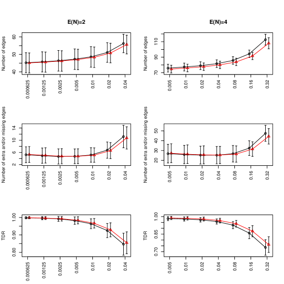
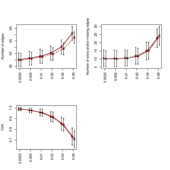
5.2 Estimation of the skeleton

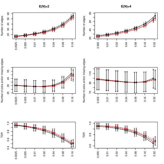
Figure 5 shows the number of edges, the number of errors, and the true discovery rate for the estimated skeletons. The figure only compares PC and PC-stable in the setting without latent variables, and RFCI and RFCI-stable in the setting with latent variables, since the modifications for the v-structures and the orientation rules do not affect the estimation of the skeleton.

Figure 5: Estimation performance of PC (circles; black line) and PC-stable (triangles; red line) for the skeleton of the CPDAGs (first column of plots), and of RFCI (circles; black line) and RFCI-stable (triangles; red line) for the skeleton of the PAGs (second column of plots), for different values of $\alpha$ ($x$-axis displayed in $\log$ scale). The results are shown as averages plus or minus one standard deviation, computed over 250 randomly generated graphs and 20 random variable orderings per graph.

(a) $\alpha=0.00125$

(b) $\alpha=0.005$

(c) $\alpha=0.02$

(d) $\alpha=0.04$

Figure 6: Estimated edges with the PC-algorithm (black) for 20 random orderings on the variables, as well as with the PC-stable algorithm (red, shown as variable ordering 21), for a random graph from the high-dimensional setting. The edges along the $x$-axes are ordered according to their presence in the 20 random orderings using the original PC-algorithm. Edges that did not occur for any of the orderings were omitted.

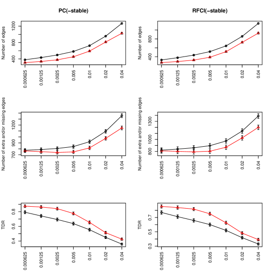
We first consider the number of estimated errors in the skeleton, shown in the first row of Figure 5. We see that PC-stable and RFCI-stable return estimated skeletons with fewer edges than PC and RFCI, for all values of $\alpha$. This can be explained by the fact that PC-stable and RFCI-stable tend to perform more tests than PC and RFCI (see also Appendix A.2). Moreover, for both algorithms smaller values of $\alpha$ lead to sparser outputs, as expected. When interpreting these plots, it is useful to know that the average number of edges in the true CPDAGs and PAGs are 1000 and 919, respectively. Thus, for both algorithms and almost all values of $\alpha$, the estimated graphs are too sparse.

The second row of Figure 5 shows that PC-stable and RFCI-stable make fewer errors in the estimation of the skeletons than PC and RFCI, for all values of $\alpha$. This may be somewhat surprising given the observations above: for most values of $\alpha$ the output of PC and RFCI is too sparse, and the output of PC-stable and RFCI-stable is even sparser. Thus, it must be that PC-stable and RFCI-stable yield a large decrease in the number of false positive edges that outweighs any increase in false negative edges.

This conclusion is also supported by the last row of Figure 5, which shows that PC-stable and RFCI-stable have a better True Discovery Rate (TDR) for all values of $\alpha$, where the TDR is defined as the proportion of edges in the estimated skeleton that are also present in the true skeleton.

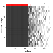
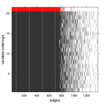
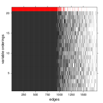
Figure 6 shows more detailed results for the estimated skeletons of PC and PC-stable for one of the 250 graphs (randomly chosen), for four different values of $\alpha$. For each value of $\alpha$ shown, PC yielded a certain number of stable edges that were present for all 20 variable orderings, but also a large number of extra edges that seem to pop in or out randomly for different orderings. The PC-stable algorithm yielded far fewer edges (shown in red), and roughly captured the edges that were stable among the different variable orderings for PC. The results for RFCI and RFCI-stable show an equivalent picture.

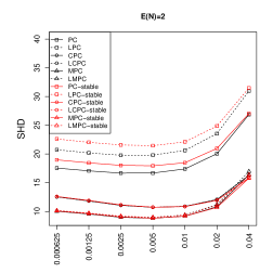
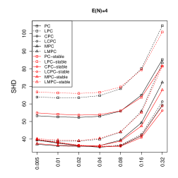
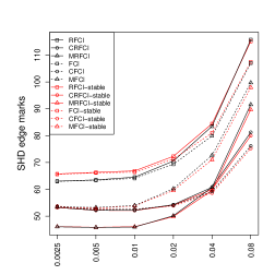
5.3 Estimation of the CPDAGs and PAGs

We now consider estimation of the CPDAG or PAG, that is, also taking into account the edge orientations. For CPDAGs, we summarize the number of estimation errors using the Structural Hamming Distance (SHD), which is defined as the minimum number of edge insertions, deletions, and flips that are needed in order to transform the estimated graph into the true one. For PAGs, we summarize the number of estimation errors by counting the number of errors in the edge marks, which we call “SHD edge marks”. For example, if an edge $X_{i}\to X_{j}$ is present in the estimated PAG but the true PAG contains $X_{i}\leftrightarrow X_{j}$, then that counts as one error, while it counts as two errors if the true PAG contains, for example, $X_{i}\leftarrow X_{j}$ or $X_{i}$ and $X_{j}$ are not adjacent.

(a) Estimation performance of (L)PC(-stable), (L)CPC(-stable), and (L)MPC(-stable) for the CPDAGs in terms of SHD.

(b) Estimation performance of RFCI(-stable), CRFCI(-stable), and MRFCI(-stable) for the PAGs in terms of SHD edge marks.

Figure 7: Estimation performance in terms of SHD for the CPDAGs and SHD edge marks for the PAGs, shown as averages over 250 randomly generated graphs and 20 random variable orderings per graph, for different values of $\alpha$ ($x$-axis displayed in $\log$ scale).

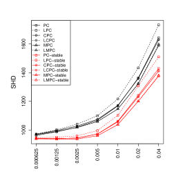
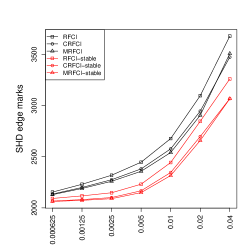
Figure 7 shows that the PC-stable and RFCI-stable versions have significantly better estimation performance than the versions with the original skeleton, for all values of $\alpha$. Moreover, MPC(-stable) and CPC(-stable) perform better than PC(-stable), as do MRFCI(-stable) and CRFCI(-stable) with respect to RFCI(-stable). Finally, for PC the idea to introduce bi-directed edges and lists in LCPC(-stable) and LMPC(-stable) seems to make little difference.

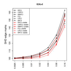
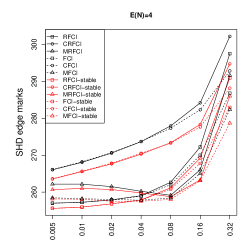
Figure 8 shows the variance in SHD for the CPDAGs, see Figure 8(a), and the variance in SHD edge marks for the PAGs, see Figure 8(b), both computed over the 20 random variable orderings per graph, and then plotted as averages over the 250 randomly generated graphs for the different values of $\alpha$. The PC-stable and RFCI-stable versions yield significantly smaller variances than their counterparts with unstabilized skeletons. Moreover, the variance is further reduced for (L)CPC-stable and (L)MPC-stable, as well as for CRFCI-stable and MRFCI-stable, as expected.

(a) Estimation performance of (L)PC(-stable), (L)CPC(-stable), and (L)MPC(-stable) for the CPDAGs in terms of the variance of SHD.

(b) Estimation performance of RFCI(-stable), CRFCI(-stable), and MRFCI(-stable) for the PAGs in terms of the variance SHD edge marks.

Figure 8: Estimation performance in terms of the variance of the SHD for the CPDAGs and SHD edge marks for the PAGs over the 20 random variable orderings per graph, shown as averages over 250 randomly generated graphs, for different values of $\alpha$ ($x$-axis displayed in $\log$ scale).

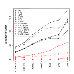
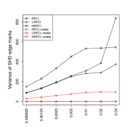
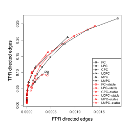
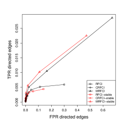
Figure 9 shows receiver operating characteristic curves (ROC) for the directed edges in the estimated CPDAGs (Figure 9(a)) and PAGs (Figure 9(b)). We see that finding directed edges is much harder in settings that allow for hidden variables, as shown by the lower true positive rates (TPR) and higher false positive rates (FPR) in Figure 9(b). Within each figure, the different versions of the algorithms perform roughly similar, and MPC-stable and MRFCI-stable yield the best ROC-curves.

(a) Estimation performance of (L)PC(-stable), (L)CPC(-stable), and (L)MPC(-stable) for the CPDAGs in terms of TPR and FPR for the directed edges.

(b) Estimation performance of RFCI(-stable), CRFCI(-stable), and MRFCI(-stable) for the PAGs in terms of TPR and FPR for the directed edges.

Figure 9: Estimation performance in terms of TPR and FPR for the directed edges in CPDAGs and PAGs, shown as averages over 250 randomly generated graphs and 20 random variable orderings per graph, where every curve is plotted with respect to the different values of $\alpha$.

6 Yeast gene expression data

We also compared the PC and PC-stable algorithms on the yeast gene expression data (Hughes et al., 2000) that were already briefly discussed in Section 1. In Section 6.1 we consider estimation of the skeleton of the CPDAG, and in Section 6.2 we consider estimation of bounds on causal effects.

We used the same pre-processed data as in Maathuis et al. (2010). These contain: (1) expression measurements of 5361 genes for 63 wild-type cultures (observational data of size $63\times 5361$), and (2) expression measurements of the same 5361 genes for 234 single-gene deletion mutant strains (interventional data of size $234\times 5361$).

6.1 Estimation of the skeleton

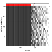
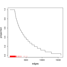
We applied PC and PC-stable to the observational data. We saw in Section 1 that the PC-algorithm yielded estimated skeletons that were highly dependent on the variable ordering, as shown in black in Figure 10 for the 26 variable orderings (the original ordering and 25 random orderings of the variables). The PC-stable algorithm does not suffer from this order-dependence, and consequently all these 26 random orderings over the variables produce the same skeleton which is shown in the figure in red. We see that the PC-stable algorithm yielded a far sparser skeleton (2086 edges for PC-stable versus 5015-5159 edges for the PC-algorithm, depending on the variable ordering). Just as in the simulations in Section 5 the order-independent skeleton from the PC-stable algorithm roughly captured the edges that were stable among the different order-dependent skeletons estimated from different variable orderings for the original PC-algorithm.

(a) As Figure 1(a), plus the edges occurring in the unique estimated skeleton using the PC-stable algorithm over the same 26 variable orderings (red, shown as variable ordering 27).

(b) The step function shows the proportion of the 26 variable orderings in which the edges were present for the original PC-algorithm, where the edges are ordered as in Figure 10(a). The red bars show the edges present in the estimated skeleton using the PC-stable algorithm.

Figure 10: Analysis of estimated skeletons of the CPDAGs for the yeast gene expression data (Hughes et al., 2000), using the PC and PC-stable algorithms. The PC-stable algorithm yields an order-independent skeleton that roughly captures the edges that were stable among the different variable orderings for the original PC-algorithm.

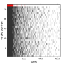
To make “captured the edges that were stable” somewhat more precise, we defined the following two sets: Set 1 contained all edges (directed edges) that were present for all 26 variable orderings using the original PC-algorithm, and Set 2 contained all edges (directed edges) that were present for at least $90\%$ of the 26 variable orderings using the original PC-algorithm. Set 1 contained 1478 edges (7 directed edges), while Set 2 contained 1700 edges (20 directed edges).

Table 3 shows how well the PC and PC-stable algorithms could find these stable edges in terms of number of edges in the estimated graphs that are present in Sets 1 and 2 (IN), and the number of edges in the estimated graphs that are not present in Sets 1 and 2 (OUT). We see that the number of estimated edges present in Sets 1 and 2 is about the same for both algorithms, while the output of the PC-stable algorithm has far fewer edges which are not present in the two specified sets.

		Edges		Directed edges
		PC-algorithm	PC-stable algorithm	PC-algorithm	PC-stable algorithm
Set 1	IN	1478 (0)	1478 (0)	7 (0)	7 (0)
	OUT	3606 (38)	607 (0)	4786 (47)	1433 (7)
Set 2	IN	1688 (3)	1688 (0)	19 (1)	20 (0)
	OUT	3396 (39)	397 (0)	4774 (47)	1420 (7)

Table 3: Number of edges in the estimated graphs that are present in Sets 1 and 2 (IN), and the number of edges in the estimated graphs that are not present in Sets 1 and 2 (OUT). The results are shown as averages (standard deviations) over the 26 variable orderings.

6.2 Estimation of causal effects

We used the interventional data as the gold standard for estimating the total causal effects of the 234 deleted genes on the remaining 5361 (see Maathuis et al. (2010)). We then defined the top $10\%$ of the largest effects in absolute value as the target set of effects, and we evaluated how well IDA (Maathuis et al., 2009, 2010) identified these effects from the observational data.

We saw in Figure 1(b) that IDA with the original PC-algorithm is highly order-dependent. Figure 11 shows the same analysis with PC-stable (solid black lines). We see that using PC-stable generally yielded better and more stable results than the original PC-algorithm. Note that some of the curves for PC-stable are worse than the reference curve of Maathuis et al. (2010) towards the beginning of the curves. This can be explained by the fact that the original variable ordering seems to be especially “lucky” for this part of the curve (cf. Figure 1(b)). There is still variability in the ROC curves in Figure 11 due to the order-dependent v-structures (because of order-dependent separating sets) and orientations in the PC-stable algorithm, but this variability is less prominent than in Figure 1(b). Finally, we see that there are 3 curves that produce a very poor fit.

Using CPC-stable and MPC-stable helps in stabilizing the outputs, and in fact all the 25 random variable orderings produce almost the same CPDAGs for both modifications. Unfortunately, these estimated CPDAGs are almost entirely undirected (around 90 directed edges among the 2086 edges) which leads to a large equivalence class and consequently to a poor performance in IDA, see the dashed black line in Figure 11 which corresponds to the 25 random variable orderings for both CPC-stable and MPC-stable algorithms.

Figure 11: ROC curves corresponding to the 25 random orderings of the variables for the analysis of yeast gene expression data (Hughes et al., 2000), where the curves are generated as in Maathuis et al. (2010) but using PC-stable (solid black lines) and MPC-stable and CPC-stable (dashed black lines) with $\alpha=0.01$. The ROC curves from Maathuis et al. (2010) (dashed blue) and the one for random guessing (dashed-dotted red) are shown as references. The resulting causal rankings are less order-dependent.

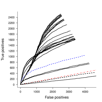
Another possible solution for the order-dependence orientation issues would be to use stability selection (Meinshausen and Bühlmann, 2010) to find the most stable orientations among the runs. In fact, Stekhoven et al. (2012) already proposed a combination of IDA and stability selection which led to improved performance when compared to IDA alone, but they used the original PC-algorithm and did not permute the variable ordering. We present here a more extensive analysis, where we consider the PC-algorithm (black lines), the PC-stable algorithm (red lines), and the MPC-stable algorithm (blue lines). Moreover, for each one of these algorithms we propose three different methods to estimate the CPDAGs and the causal effects: (1) use the original ordering of the variables (solid lines); (2) use the same methodology used in Stekhoven et al. (2012) with 100 stability selection runs but without permuting the variable orderings (labelled as + SS; dashed lines); and (3) use the same methodology used in Stekhoven et al. (2012) with 100 stability selection runs but permuting the variable orderings in each run (labelled as + SSP; dotted lines). The results are shown in Figure 12 where we investigate the performance for the top 20000 effects instead of the 5000 as in Figures 1(b) and 11.

Figure 12: Analysis of the yeast gene expression data (Hughes et al., 2000) for PC, PC-stable, and MPC-stable algorithms using the original ordering over the variables (solid lines), using 100 runs stability selection without permuting the variable orderings, labelled as + SS (dashed lines), and using 100 runs stability selection with permuting the variable orderings, labelled as + SSP (dotted lines). The grey line labelled as RG represents the random guessing.

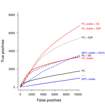
We see that PC with stability selection and permuted variable orderings (PC + SSP) loses some performance at the beginning of the curve when compared to PC with standard stability selection (PC + SS), but it has much better performance afterwards. The PC-stable algorithm with the original variable ordering performs very similar to PC plus stability selection (PC + SS) along the whole curve. Moreover, PC-stable plus stability selection (PC-stable + SS and PC-stable + SSP), loses a bit at the beginning of the curves but picks up much more signal later on in the curve. It is interesting to note that for PC-stable with stability selection, it makes little difference if the variable orderings are further permuted or not, even though PC-stable is not fully order-independent (see Figure 11). In fact, PC-stable plus stability selection (with or without permuted variable orderings) produces the best fit over all results.

7 Discussion

Due to their computational efficiency, constraint-based causal structure learning algorithms are often used in sparse high-dimensional settings. We have seen, however, that especially in these settings the order-dependence in these algorithms is highly problematic.

In this paper, we investigated this issue systematically, and resolved the various sources of order-dependence. There are of course many ways in which the order-dependence issues could be resolved, and we designed our modifications to be as simple as possible. Moreover, we made sure that existing high-dimensional consistency results for PC-, FCI- and RFCI-algorithms remain valid for their modifications under the same conditions. We showed that our proposed modifications yield improved and more stable estimation in sparse high-dimensional settings for simulated data, while their performances are similar to the performances of the original algorithms in low-dimensional settings.

Additionally to the order-dependence discussed in this paper, there is another minor type of order-dependence in the sense that the output of these algorithms also depends on the order in which the final orientation rules for the edges are applied. The reason is that an edge(mark) could be eligible for orientation by several orientation rules, and might be oriented differently depending on which rule is applied first. In our analyses, we have always used the original orderings in which the rules were given.

Compared to the adaptation of Cano et al. (2008), the modifications we propose are much simpler and we made sure that they preserve existing soundness, completeness, and high-dimensional consistency results. Finally, our modifications can be easily used together with other adaptations of constraint-based algorithms, for example hybrid versions of PC with score-based methods Singh and Valtorta (1993); Spirtes and Meek (1995); van Dijk et al. (2003) or the PC^∗ algorithm (Spirtes et al., 2000, Section 5.4.2.3).

All software is implemented in the R-package pcalg (Kalisch et al., 2012).

A Additional simulation results

We now present additional simulation results for low-dimensional settings (Appendix A.1), high-dimensional settings (Appendix A.2) and medium-dimensional settings (Appendix A.3).

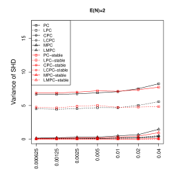
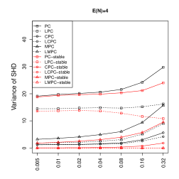
A.1 Estimation performance in low-dimensional settings

We considered the estimation performance in low-dimensional settings with less sparse graphs.

For the scenario without latent variables, we generated 250 random weighted DAGs with $p=50$ and $E(N)=\{2,4\}$, as described in Section 5.1. For each weighted DAG we generated an i.i.d. sample of size $n=1000$. We then estimated each graph for 50 random orderings of the variables, using the sample versions of (L)PC(-stable), (L)CPC(-stable), and (L)MPC(-stable) at levels $\alpha\in\{0.000625,0.00125,0.0025,0.005,0.01,0.02,0.04\}$ for $E(N)=2$ and $\alpha\in\{0.005,0.01,0.02,0.04,0.08,0.16,0.32\}$ for $E(N)=4$ for the partial correlation tests. Thus, for each randomly generated graph, we obtained 50 estimated CPDAGs from each algorithm, for each value of $\alpha$. Figure 13 shows the estimation performance of PC (circle; black line) and PC-stable (triangles; red line) for the skeleton. Figure 14 shows the estimation performance of all modifications of PC and PC-stable with respect to the CPDAGs in terms of SHD, and in terms of the variance of the SHD over the 50 random variable orderings per graph.

Figure 13: Estimation performance of PC (circles; black line) and PC-stable (triangles; red line) for the skeleton of the CPDAGs, for different values of $\alpha$ ($x$-axis displayed in $\log$ scale) in both low-dimensional settings. The results are shown as averages plus or minus one standard deviation, computed over 250 randomly generated graphs and 50 random variable orderings per graph, and slightly shifted up and down from the real values of $\alpha$ for a better visualization.

Figure 14: Estimation performance of (L)PC(-stable), (L)CPC(-stable), and (L)MPC(-stable) for the CPDAGs in the low-dimensional settings, for different values of $\alpha$. The first row of plots shows the performance in terms of SHD, shown as averages over 250 randomly generated graphs and 50 random variable orderings per graph. The second row of plots shows the performance in terms of the variance of the SHD over the 50 random variable orderings per graph, shown as averages over 250 randomly generated graphs.

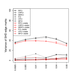
For the scenario with latent variables, we generated 120 random weighted DAGs with $p=50$ and $E(N)=2$, as described in Section 5.1. For each DAG we generated an i.i.d. sample size of $n=1000$. To assess the impact of latent variables, we randomly defined in each DAG half of the variables that have no parents and at least two children to be latent. We then estimated each graph for 20 random orderings of the observed variables, using the sample versions of FCI(-stable), CFCI(-stable), MFCI(-stable), RFCI(-stable), CRFCI(-stable), and MRFCI(-stable) at levels $\alpha\in\{0.0025,0.005,0.01,0.02,0.04,0.08\}$ for the partial correlation tests. Thus, for each randomly generated graph, we obtained 20 estimated PAGs from each algorithm, for each value of $\alpha$. Figure 15 shows the estimation performance of FCI (circles; black dashed line), FCI-stable (triangles; red dashed line), RFCI (circles; black solid line), and RFCI-stable (triangles; red solid line) for the skeleton. Figure 16 shows the estimation performance for the PAGs in terms of SHD edge marks, and in terms of the variance of the SHD edge marks over the 20 random variable orderings per graph.

Figure 15: Estimation performance of FCI (circles; black dashed line), FCI-stable (triangles; red dashed line), RFCI (circles; black solid line), and RFCI-stable (triangles; red solid line), for the skeleton of the PAGs for different values of $\alpha$ ($x$-axis displayed in $\log$ scale) in the low-dimensional setting. The results are shown as averages plus or minus one standard deviation, computed over 120 randomly generated graphs and 20 random variable orderings per graph, and slightly shifted up and down from the real values of $\alpha$ for a better visualization.

Figure 16: Estimation performance of the modifications of FCI(-stable) and RFCI(-stable) for the PAGs in the low-dimensional setting, for different values of $\alpha$. The left panel shows the performance in terms of SHD edge marks, shown as averages over 120 randomly generated graphs and 20 random variable orderings per graph. The right panel shows the performance in terms of the variance of the SHD edge marks over the 20 random variable orderings per graph, shown as averages over 120 randomly generated graphs.

Regarding the skeletons of the CPDAGs and PAGs, the estimation performances between PC and PC-stable, as well as between (R)FCI and (R)FCI-stable are basically indistinguishable for all values of $\alpha$. However, Figure 15 shows that FCI(-stable) returns graphs with slightly fewer edges than RFCI(-stable), for all values of $\alpha$. This is related to the fact that FCI(-stable) tends to perform more tests than RFCI(-stable).

Regarding the CPDAGs and PAGs, the performance of the modifications of PC and (R)FCI (black lines) are very close to the performance of PC-stable and (R)FCI-stable (red lines). Moreover, CPC(-stable) and MPC(-stable) as well as C(R)FCI(-stable) and M(R)FCI(-stable) perform better in particular in reducing the variance of the SHD and SHD edge marks, respectively. This indicates that most of the order-dependence in the low-dimensional setting is in the orientation of the edges.

We also note that in all proposed measures there are only small differences between modifications of FCI and of RFCI.

A.2 Number of tests and computing time

We consider the number of tests and the computing time of PC and PC-stable in the high-dimensional setting described in Section 5.1.

One can easily deduce that Step 1 of the PC- and PC-stable algorithms perform the same number of tests for $\ell=0$, because the adjacency sets do not play a role at this stage. Moreover, for $\ell=1$ PC-stable performs at least as many tests as PC, since the adjacency sets $a(X_{i})$ (see Algorithm 4.1) are always supersets of the adjacency sets $\text{adj}(X_{i})$ (see Algorithm 3.2). For larger values of $\ell$, however, it is difficult to analyze the number of tests analytically.

Table 4 therefore shows the average number of tests that were performed by Step 1 of the two algorithms, separated by size of the conditioning set, where we considered the high-dimensional setting with $\alpha=0.04$ (see Section 5.2) since this was most computationally intensive. As expected the number of marginal correlation tests was identical for both algorithms. For $\ell=1$, PC-stable performed slightly more than twice as many tests as PC, amounting to about $1.36\times 10^{5}$ additional tests. For $\ell=2$, PC-stable performed more tests than PC, amounting to $3.4\times 10^{3}$. For larger values of $\ell$, PC-stable performed fewer tests than PC, since the additional tests for $\ell=1$ and $\ell=2$ lead to a sparser skeleton. However, since PC also performed relatively few tests for larger values of $\ell$, the absolute difference in the number of tests for large $\ell$ is rather small. In total, PC-stable performed about $1.39\times 10^{5}$ more tests than PC.

	PC-algorithm	PC-stable algorithm
$\ell=0$	$5.21\times 10^{5}$ ($1.95\times 10^{2}$)	$5.21\times 10^{5}$ ($1.95\times 10^{2}$)
$\ell=1$	$1.29\times 10^{5}$ ($2.19\times 10^{3}$)	$2.65\times 10^{5}$ ($4.68\times 10^{3}$)
$\ell=2$	$1.10\times 10^{4}$ ($5.93\times 10^{2}$)	$1.44\times 10^{4}$ ($8.90\times 10^{2}$)
$\ell=3$	$1.12\times 10^{3}$ ($1.21\times 10^{2}$)	$5.05\times 10^{2}$ ($8.54\times 10^{1}$)
$\ell=4$	$9.38\times 10^{1}$ ($2.86\times 10^{1}$)	$3.08\times 10^{1}$ ($1.78\times 10^{1}$)
$\ell=5$	$2.78\times 10^{0}$ ($4.53\times 10^{0}$)	$0.65\times 10^{0}$ ($1.94\times 10^{0}$)
$\ell=6$	$0.02\times 10^{0}$ ($0.38\times 10^{0}$)	-
Total	$6.62\times 10^{5}$ ($2.78\times 10^{3}$)	$8.01\times 10^{5}$ ($5.47\times 10^{3}$)

Table 4: Number of tests performed by Step 1 of the PC and PC-stable algorithms for each size of the conditioning sets $\ell$, in the high-dimensional setting with $p=1000$, $n=50$ and $\alpha=0.04$. The results are shown as averages (standard deviations) over 250 random graphs and 20 random variable orderings per graph.

Table 5 shows the average runtime of the PC- and PC-stable algorithms. We see that PC-stable is somewhat slower than PC for all values of $\alpha$, which can be explained by the fact that PC-stable tends to perform a larger number of tests (cf. Table 4).

	PC-algorithm	PC-stable algorithm	PC / PC-stable
$\alpha=0.000625$	111.79 (7.54)	115.46 (7.47)	0.97
$\alpha=0.00125$	110.13 (6.91)	113.77 (7.07)	0.97
$\alpha=0.025$	115.90 (12.18)	119.67 (12.03)	0.97
$\alpha=0.05$	116.14 (9.50)	119.91 (9.57)	0.97
$\alpha=0.01$	121.02 (8.61)	125.81 (8.94)	0.96
$\alpha=0.02$	131.42 (13.98)	139.54 (14.72)	0.94
$\alpha=0.04$	148.72 (14.98)	170.49 (16.31)	0.87

Table 5: Run time in seconds (computed on an AMD Opteron(tm) Processor 6174 using R 2.15.1.) of PC and PC-stable for the high-dimensional setting with $p=1000$ and $n=50$. The results are shown as averages (standard deviations) over 250 random graphs and 20 random variable orderings per graph.

A.3 Estimation performance in settings where $p=n$

Finally, we consider two settings for the scenario with latent variables, where we generated 250 random weighted DAGs with $p=50$ and $E(N)=\{2,4\}$, as described in Section 5.1. For each DAG we generated an i.i.d. sample size of $n=50$. We again randomly defined in each DAG half of the variables that have no parents and at least two children to be latent. We then estimated each graph for 50 random orderings of the observed variables, using the sample versions of FCI(-stable), CFCI(-stable), MFCI(-stable), RFCI(-stable), CRFCI(-stable), and MRFCI(-stable) at levels $\alpha\in\{0.0025,0.005,0.01,0.02,0.04,0.08,0.16\}$ for $E(N)=2$ and $\alpha\in\{0.005,0.01,0.02,0.04,0.08,0.16,0.32\}$ for $E(N)=4$. Thus, for each randomly generated graph, we obtained 50 estimated PAGs from each algorithm, for each value of $\alpha$.

Figure 17 shows the estimation performance for the skeleton. The (R)FCI-stable versions (red lines) lead to slightly sparser graphs and slightly better performance in TDR than (R)FCI versions (black lines) in both settings.

Figure 17: Estimation performance of FCI (circles; black dashed line), FCI-stable (triangles; red dashed line), RFCI (circles; black solid line), and RFCI-stable (triangles; red solid line), for the skeleton of the PAGs for different values of $\alpha$ ($x$-axis displayed in $\log$ scale) in two settings where $p=n$. The results are shown as averages plus or minus one standard deviation, computed over 250 randomly generated graphs and 50 random variable orderings per graph, and slightly shifted up and down from the real values of $\alpha$ for a better visualization.

Figures 18 shows the estimation performance of all modifications of (R)FCI with respect to the PAGs in terms of SHD edge marks, and in terms of the variance of the SHD edge marks over the 50 random variable orderings per graph. The (R)FCI-stable versions produce a better fit than the (R)FCI versions. Moreover, C(R)FCI(-stable) and M(R)FCI(-stable) perform similarly for sparse graphs and they improve the fit, while in denser graphs M(R)FCI(-stable) still improves the fit and it performs much better than C(R)FCI(-stable) for the SHD edge marks. Again we see little difference between modifications of RFCI and FCI with respect to all measures.

Figure 18: Estimation performance of the modifications of FCI(-stable) and RFCI(-stable) for the PAGs in settings where $p=n$, for different values of $\alpha$. The first row of plots shows the performance in terms of SHD edge marks, shown as averages over 250 randomly generated graphs and 50 random variable orderings per graph. The second row of plots shows the performance in terms of the variance of the SHD edge marks over the 50 random variable orderings per graph, shown as averages over 250 randomly generated graphs.

References

- Andersson et al. (1997) S. A. Andersson, D. Madigan, and M. D. Perlman. A characterization of Markov equivalence classes for acyclic digraphs. Ann. Statist., 25(2):505–541, 1997.
- Cano et al. (2008) A. Cano, M. Gómez-Olmedo, and S. Moral. A score based ranking of the edges for the PC algorithm. In Proceedings of the Fourth European Workshop on Probabilistic Graphical Models, pages 41–48, 2008.
- Chickering (2002) D.M. Chickering. Learning equivalence classes of Bayesian-network structures. J. Mach. Learn. Res., 2:445–498, 2002.
- Claassen et al. (2013) Tom Claassen, Joris Mooij, and Tom Heskes. Learning sparse causal models is not NP-hard. In Proceedings of the 29th Conference on Uncertainty in Artificial Intelligence, 2013. To appear.
- Colombo et al. (2012) D. Colombo, M.H. Maathuis, M. Kalisch, and T.S. Richardson. Learning high-dimensional directed acyclic graphs with latent and selection variables. Ann. Statist., 40(1):294–321, 2012. ISSN 0090-5364.
- Dash and Druzdzel (1999) D. Dash and M.J. Druzdzel. A hybrid anytime algorithm for the construction of causal models from sparse data. In Proceedings of the Fifteenth Conference on Uncertainty on Artificial Intelligence (UAI-99), pages 142–149. Morgan Kaufmann Publishers, Inc., 1999.
- Dawid (1980) A. P. Dawid. Conditional independence for statistical operations. Ann. Statist., 8:598–617, 1980.
- Harris and Drton (2012) N. Harris and M. Drton. PC algorithm for gaussian copula graphical models. arXiv preprint arXiv:1207.0242, 2012.
- Hughes et al. (2000) T.R. Hughes, M.J. Marton, A.R. Jones, C.J. Roberts, R. Stoughton, C.D. Armour, H.A. Bennett, E. Coffey, H. Dai, Y.D. He, and et al. Functional discovery via a compendium of expression profiles. Cell, 102(1):109–126, 2000.
- Kalisch and Bühlmann (2007) M. Kalisch and P. Bühlmann. Estimating high-dimensional directed acyclic graphs with the PC-algorithm. J. Mach. Learn. Res., 8:613–636, 2007.
- Kalisch et al. (2010) M. Kalisch, B.A.G. Fellinghauer, E. Grill, M.H. Maathuis, U. Mansmann, P. Bühlmann, and G. Stucki. Understanding human functioning using graphical models. BMC Medical Research Methodology, 10(1):14, 2010.
- Kalisch et al. (2012) M. Kalisch, M. Mächler, D. Colombo, M.H. Maathuis, and P. Bühlmann. Causal inference using graphical models with the R package pcalg. Journal of Statistical Software, 47(11):1–26, 2012.
- Maathuis et al. (2009) M.H. Maathuis, M. Kalisch, and P. Bühlmann. Estimating high-dimensional intervention effects from observational data. Ann. Statist., 37(6A):3133–3164, 2009.
- Maathuis et al. (2010) M.H. Maathuis, D. Colombo, M. Kalisch, and P. Bühlmann. Predicting causal effects in large-scale systems from observational data. Nature Methods, 7(4):247–248, 2010.
- Meek (1995) C. Meek. Causal inference and causal explanation with background knowledge. In Proceedings of the Eleventh Conference on Uncertainty in Artificial Intelligence (UAI-95), pages 403–411. Morgan Kaufmann Publishers, Inc., 1995.
- Meinshausen and Bühlmann (2010) N. Meinshausen and P. Bühlmann. Stability selection. Journal of the Royal Statistical Society: Series B (Statistical Methodology), 72(4):417–473, 2010.
- Nagarajan et al. (2010) R. Nagarajan, S. Datta, M. Scutari, M. Beggs, G. Nolen, and C. Peterson. Functional relationships between genes associated with differentiation potential of aged myogenic progenitors. Frontiers in Physiology, 1(160), 2010.
- Pearl (2000) J. Pearl. Causality. Models, reasoning, and inference. Cambridge University Press, Cambridge, 2000.
- Pearl (2009) J. Pearl. Causal inference in statistics: An overview. Statistics Surveys, 3:96–146, 2009.
- Ramsey et al. (2006) Joseph Ramsey, Jiji Zhang, and Peter Spirtes. Adjacency-faithfulness and conservative causal inference. In Proceedings of the 22nd Annual Conference on Uncertainty in Artificial Intelligence, Arlington, VA, 2006. AUAI Press.
- Richardson (1996) Thomas S. Richardson. A discovery algorithm for directed cyclic graphs. In Proceedings of the Twelfth international conference on Uncertainty in artificial intelligence, pages 454–461. Morgan Kaufmann Publishers Inc., 1996.
- Singh and Valtorta (1993) M. Singh and M. Valtorta. An algorithm for the construction of bayesian network structures from data. In Proceedings of the Ninth International Conference on Uncertainty in Artificial Intelligence (UAI-93), pages 259–265. Morgan Kaufmann Publishers, Inc., 1993.
- Spirtes and Meek (1995) P. Spirtes and C. Meek. Learning bayesian networks with discrete variables from data. In Proceeding of the First International Conference on Knowledge Discovery and Data Mining, pages 294–299, Menlo Park, CA: AAAI, 1995.
- Spirtes et al. (1999) P. Spirtes, C. Meek, and Thomas S. Richardson. An algorithm for causal inference in the presence of latent variables and selection bias. In Computation, Causation and Discovery, pages 211–252. MIT Press, 1999.
- Spirtes et al. (2000) P. Spirtes, C. Glymour, and R. Scheines. Causation, Prediction, and Search. MIT Press, Cambridge, second edition, 2000.
- Spirtes (2001) Peter Spirtes. An anytime algorithm for causal inference. In Proc. of the Eighth International Workshop on Artificial Intelligence and Statistics, pages 213–221, San Francisco, 2001. Morgan Kaufmann.
- Spirtes et al. (1993) Peter Spirtes, Clark Glymour, and Richard Scheines. Causation, prediction, and search, volume 81 of Lecture Notes in Statistics. Springer-Verlag, New York, 1993. doi: 10.1007/978-1-4612-2748-9.
- Stekhoven et al. (2012) D.J. Stekhoven, I. Moraes, G. Sveinbjörnsson, L. Hennig, M.H. Maathuis, and P. Bühlmann. Causal stability ranking. Bioinformatics, 2012.
- van Dijk et al. (2003) S. van Dijk, L.C. can der Gaag, and D. Thierens. A skeleton-based approach to learning bayesian networks from data. In Proceedings of the Seventh Conference on Principles and Practice of Knowledge Discovery in Databases (PKDD 2003), pages 132–143. Springer Verlag, 2003.
- Zhang (2008) Jiji Zhang. On the completeness of orientation rules for causal discovery in the presence of latent confounders and selection bias. Artificial Intelligence, 172:1873–1896, 2008.
- Zhang et al. (2011) X. Zhang, X.M. Zhao, K. He, L. Lu, Y. Cao, J. Liu, J.K. Hao, Z.P. Liu, and L. Chen. Inferring gene regulatory networks from gene expression data by pc-algorithm based on conditional mutual information. Bioinformatics, 2011.