Sunyaev-Zeldovich signal processing and temperature-velocity moment method for individual clusters

Jens Chluba1,2, Eric Switzer1,3, Kaylea Nelson4, Daisuke Nagai4,5,6

1 Canadian Institute for Theoretical Astrophysics, 60 St. George Street, Toronto, ON M5S 3H8, Canada
2 Johns Hopkins University, Department of Physics and Astronomy, Bloomberg 439, 3400 N. Charles St., Baltimore, MD 21218
3 Kavli Institute for Cosmological Physics, University of Chicago, 933 East 56th Street, Chicago, IL 60637, USA
4 Department of Astronomy, Yale University, New Haven, CT 06520, U.S.A.
5 Department of Physics, Yale University, New Haven, CT 06520, U.S.A.
6 Yale Center for Astronomy & Astrophysics, Yale University, New Haven, CT 06520, U.S.A
E-mail: jchluba@pha.jhu.edu
(Accepted 2013 January 16. Received 2013 January 09; in original form 2012 November 14)
Abstract

Future high resolution, high sensitivity Sunyaev-Zeldovich (SZ) observations of individual clusters will provide an exciting opportunity to answer specific questions about the dynamical state of the intra-cluster medium (ICM). In this paper we develop a new method that clearly shows the connection of the SZ signal with the underlying cluster model. We include relativistic temperature and kinematic corrections in the single-scattering approximation, allowing studies of hot clusters. In our approach, particular moments of the temperature and velocity field along the line-of-sight determine the precise spectral shape and morphology of the SZ signal. We illustrate how to apply our method to different cluster models, highlighting parameter degeneracies and instrumental effects that are important for interpreting future high-resolution SZ data. Our analysis shows that line-of-sight temperature variations can introduce significant biases in the derived SZ temperature and peculiar velocity. We furthermore discuss how the position of the SZ null is affected by the cluster’s temperature and velocity structure. Our computations indicate that the SZ signal around the null alone is rather insensitive to different cluster models and that high frequency channels add a large leverage in this respect. We also apply our method to recent high sensitivity SZ data of the Bullet cluster, showing how the results can be linked to line-of-sight variations in the electron temperature. The tools developed here as part of SZpack should be useful for analyzing high-resolution SZ data and computing SZ maps from simulated clusters.

keywords:
Cosmology: cosmic microwave background – theory – observations

1 Introduction

Since the early measurements of the SZ effect in the 80’s and 90’s (e.g., Birkinshaw et al., 1984, 1991; Lamarre et al., 1998; Hughes & Birkinshaw, 1998) the observational possibilities in the microwave band have evolved at an impressive rate. Today the thermal SZ (thSZ) effect (Zeldovich & Sunyaev, 1969) is routinely detected for several hundred galaxy clusters out to redshift z1similar-to-or-equals𝑧1z\simeq 1 (Benson et al., 2004; Marriage et al., 2011; Williamson et al., 2011; Planck Collaboration et al., 2011), and in some cases evidence for the presence of the smaller kinematic SZ (kSZ) effect (Sunyaev & Zeldovich, 1980) is found (Benson et al., 2003; Korngut et al., 2011; Mroczkowski et al., 2012; Hand et al., 2012).

SZ cluster observations are a powerful cosmological tool (see Rephaeli, 1995a; Birkinshaw, 1999; Carlstrom et al., 2002; Komatsu & Seljak, 2002, for overview), but to realize their full constraining power for precision cosmology it is critical to understand the structure and evolution of the intra-cluster medium (ICM) in more detail. Already now a number of high-resolution SZ experiments, including ALMA111Atacama Large Millimeter/submillimeter Array, CARMA222Combined Array for Research in Millimeter-wave Astronomy, CCAT333Cornell Caltech Atacama Telescope, and MUSTANG444MUltiplexed Squid TES Array at Ninety GHz, are underway or planned, promising a dramatic increase in sensitivities, spatial resolution, and spectral coverage over the next few years. Current generation high-resolution SZ observations of individual clusters have already revealed rich phenomena (e.g., shocks, substructures, relativistic particles) in the atmospheres of merging clusters (e.g., Komatsu et al., 2001; Kitayama et al., 2004; Colafrancesco et al., 2011; Korngut et al., 2011; Menanteau et al., 2012; Mroczkowski et al., 2012; Zemcov et al., 2012; Prokhorov & Colafrancesco, 2012). Upcoming SZ experiments should enable a host of exciting measurements of important physical processes that shape the properties of the ICM and their evolution, including the electron temperature (Pointecouteau et al., 1998; Hansen et al., 2002), the peculiar velocity of the cluster, internal bulk and turbulent gas motions (e.g., Chluba & Mannheim, 2002; Nagai et al., 2003; Sunyaev et al., 2003; Diego et al., 2003), and non-equilibrium electrons produced by merger and accretion shocks (Markevitch & Vikhlinin, 2007; Rudd & Nagai, 2009).

These encouraging prospects also raise a number of important problems that must be addressed before the rich information contained in the future SZ data can be fully exploited. One is simply related to the precise and fast computation of the SZ signal given basic parameters of the scattering medium, such as the Thomson scattering optical depth, τ𝜏\tau, the electron temperature, Tesubscript𝑇eT_{\rm e}, and bulk velocity, βcsubscript𝛽c\beta_{\rm c}, while accounting for relativistic temperature and kinematic corrections. Previously, this issue has been addressed by several groups (Rephaeli, 1995b; Challinor & Lasenby, 1998; Itoh et al., 1998; Sazonov & Sunyaev, 1998; Nozawa et al., 1998a; Challinor & Lasenby, 1999; Chluba et al., 2005) by means of Taylor expansions for the SZ signal. While the evaluation of these expansions is very fast, they are limited to rather low temperature gas (Fig. 2 shows that for Te13keVgreater-than-or-equivalent-tosubscript𝑇e13keVT_{\rm e}\gtrsim 13\,{\rm keV} this approach breaks down). One alternative is direct numerical integration of the Boltzmann collision term making use of the symmetries of the scattering problem (Wright, 1979; Dolgov et al., 2001; Nozawa et al., 2009; Poutanen & Vurm, 2010), but this is time-consuming and not well-suited for extensive parameter estimations or computations of the SZ signal from simulated clusters. On the other hand, a fast but not as precise and flexible approach is simple tabulation of the SZ signal or the use of convenient fitting function (Nozawa et al., 2000; Itoh & Nozawa, 2004; Shimon & Rephaeli, 2004).

Recently, Chluba et al. (2012, CNSN in the following) developed a method in the middle of these extremes. In their work, a new set of frequency-dependent basis functions was computed numerically to allow very fast and precise calculation of the SZ signal. The basis functions are informed by the underlying physics of the scattering problem and thus are ideally suited for future SZ signal processing and parameter estimation. The associated routines are part of SZpack555www.Chluba.de/SZpack; (now also including Python bindings). However, several extensions are required. Firstly, so far high precision (relative accuracy 0.001%similar-to-or-equalsabsentpercent0.001\simeq 0.001\%) calculations with SZpack were limited to Te25keVless-than-or-similar-tosubscript𝑇e25keVT_{\rm e}\lesssim 25\,{\rm keV}. This problem can be easily overcome using the method of CNSN by appropriate extensions of the basis functions, as we explain in Sect. 2.4. With SZpack v1.1, which is presented here, it is now possible to compute the SZ signal for Te75keVless-than-or-similar-tosubscript𝑇e75keVT_{\rm e}\lesssim 75\,{\rm keV} and βc0.01less-than-or-similar-tosubscript𝛽c0.01\beta_{\rm c}\lesssim 0.01 to 0.001%similar-to-or-equalsabsentpercent0.001\simeq 0.001\% relative precision at practically no computational cost. This precision and range of parameters covers all physically relevant cases and hence provides an important preparation for SZ parameter estimation without significant limitations.

Secondly, line-of-sight variations of the temperature and velocity field (with any of the aforementioned methods) can only be accounted for by means of additional 1-dimensional integrals; this again makes extensive SZ parameter estimation expensive. Especially when computing the SZ signal from cluster simulations the problem becomes very demanding, even if evaluation for single gas parameters (τ𝜏\tau, Tesubscript𝑇eT_{\rm e}, and βcsubscript𝛽c\beta_{\rm c}) is extremely fast. Here we reformulate the representation of the SZ signal to overcome this limitation. We utilize that in the single-scattering approximation, frequency-dependent terms can be separated from temperature- and velocity-dependent contributions (Sect. 2). This implies that the SZ signal for a given cluster model can be calculated using appropriate moments of the temperature and velocity field. While this means that a finite number of 1-dimensional integrals along different lines-of-sight have to be evaluated, this separation still greatly reduces the computational burden because afterward the SZ signal at any frequency can be computed as simple matrix multiplication.

While the method developed in Sect. 2 is both precise and fast, delivering quasi-exact results for the SZ signal through different lines-of-sight for any cluster atmosphere, in the future analysis of high resolution, high sensitivity SZ data another simplification is possible. In Sect. 3, we show that for typical cluster models the smoothness of the temperature and velocity profiles allows minimizing the number of parameters needed to accurately describe the SZ signal, resulting in a second set of moments that are related to the line-of-sight temperature and velocity dispersions and higher order statistics (see Eq. (18) for instance). The associated expansion of the SZ signal around the mean becomes perturbative and the number of moments needed to describe the SZ signal depends directly on the observational sensitivity.

Our formulation furthermore allows direct separation of frequency-dependent from spatially varying terms, providing a clear link between morphological changes of the SZ signal and cluster parameters. For example, the presence of large-scale, post-merger cluster rotation can introduce a bipolar kSZ signal, which is related to a spatially varying average line-of-sight velocity. The superposition of thSZ with this rotational kSZ implies small frequency-dependent changes of the clusters morphology (Chluba & Mannheim, 2002). Similarly, variations of the electron temperature along the line-of-sight introduce morphological effects (as also pointed out more recently by Prokhorov et al., 2011), and as we explain here, spatial variations of temperature and velocity moments are the source of these morphological changes. The moments therefore constitute the main observables of high-resolution, high-sensitivity SZ observations and their interpretation is the main challenge for future SZ parameter estimation and in the reconstruction of the cluster’s temperature and velocity structure.

Armed with these tools, we address a number of questions that are related to the effect of temperature and velocity variations on the SZ signal, with particular focus on parameter degeneracies and instrumental aspects. For example, we explicitly discuss the effect of angular resolution and frequency filters on the SZ signal, as well as different corrections to the location of the SZ null. All these aspects, if ignored, lead to biases in the deduced cluster parameters. We illustrate this for several examples, using both mock SZ measurements as well as recent SZ data. We furthermore develop several tools for SZ parameter estimation which are now part of SZpack. These should be useful for computing the SZ signal from cluster simulations and in the analysis of future high resolution, high sensitivity SZ measurements.

2 Computing the SZ signal using temperature and velocity moments

In this section we introduce the new temperature-velocity moment method to compute the SZ signal for general cluster atmospheres. This section is rather technical and mainly for readers interested in the computational details.

The SZ effect is caused by the scattering of CMB photons by moving electrons. For a small volume element of scattering electrons the SZ signal only depends on the electron temperature, Tesubscript𝑇eT_{\rm e}, their total bulk velocity, 𝜷csubscript𝜷c{{\boldsymbol{\beta}}_{\rm c}}, the direction cosine of this velocity with respect to the line-of-sight666In the following bold font denotes 3-dimensional vectors and an additional hat means that it is normalized to unity., μc=𝜷^c𝜸^subscript𝜇csubscript^𝜷c^𝜸\mu_{\rm c}={\hat{{\boldsymbol{\beta}}}_{\rm c}}\cdot{\hat{\boldsymbol{\gamma}}}, and the Thomson optical depth of the scattering volume element, ΔτΔ𝜏\Delta\tau. Both Tesubscript𝑇eT_{\rm e} and ΔτΔ𝜏\Delta\tau are defined in the rest frame of the scattering volume element, while 𝜷csubscript𝜷c{{\boldsymbol{\beta}}_{\rm c}} is defined with respect to the CMB rest frame.

For now, we shall assume that the observer is at rest in the CMB frame. The conversion of the aforementioned parameters to the SZ signal can be expressed as ΔI(x)=ΔτFSZ(x,Te,βc,μc)Δ𝐼𝑥Δ𝜏subscript𝐹SZ𝑥subscript𝑇esubscript𝛽csubscript𝜇c\Delta I(x)=\Delta\tau\,F_{\rm SZ}(x,T_{\rm e},\beta_{\rm c},\mu_{\rm c}), where FSZsubscript𝐹SZF_{\rm SZ} is a non-linear function and x=hν/kT0𝑥𝜈𝑘subscript𝑇0x=h\nu/kT_{0} with CMB temperature T0=2.726Ksubscript𝑇02.726KT_{0}=2.726\,{\rm K} (Fixsen et al., 1996; Fixsen & Mather, 2002). The change in the CMB intensity can be further rewritten as

ΔI(x)Δ𝐼𝑥\displaystyle\Delta I(x) ΔτIox3[Y(x,Te)+βc2M(x,Te)\displaystyle\approx\Delta\tau\,{I_{\rm o}\,x^{3}}\left[Y(x,T_{\rm e})+{\beta^{2}_{\rm c}}M(x,T_{\rm e})\right.
+βcP1(μc)D(x,Te)+βc2P2(μc)Q(x,Te)],\displaystyle\quad\qquad\left.+\beta_{\rm c}P_{1}(\mu_{\rm c})\,D(x,T_{\rm e})+{\beta^{2}_{\rm c}}P_{2}(\mu_{\rm c})\,Q(x,T_{\rm e})\right], (1)

where Io=(2h/c2)(kT0/h)3270MJysr1subscript𝐼o2superscript𝑐2superscript𝑘subscript𝑇03270MJysuperscriptsr1I_{\rm o}=(2h/c^{2})(kT_{0}/h)^{3}\approx 270\,{\rm MJy\,sr^{-1}} and Pl(x)subscript𝑃𝑙𝑥P_{l}(x) denote Legendre polynomials. The term Y(x,Te)𝑌𝑥subscript𝑇eY(x,T_{\rm e}) describes the purely thermal SZ effect with temperature corrections included, while terms βcproportional-toabsentsubscript𝛽c\propto\beta_{\rm c} are related to kinematic effects.

From previous analysis of the SZ effect, it is furthermore clear that the functions Y(x,Te)𝑌𝑥subscript𝑇eY(x,T_{\rm e}), M(x,Te)𝑀𝑥subscript𝑇eM(x,T_{\rm e}), D(x,Te)𝐷𝑥subscript𝑇eD(x,T_{\rm e}) and Q(x,Te)𝑄𝑥subscript𝑇eQ(x,T_{\rm e}) can all be described using an appropriate set of frequency-dependent basis functions and temperature-dependent coefficients, where the latter encode the spatial dependence. The integrated SZ signal along a given line-of-sight is therefore determined by appropriate moments of the cluster’s temperature and velocity field. These contain the desired information about the cluster gas and structure; as such they define the observables of the SZ measurement, and the aim will be to use the moments to learn about the cluster gas.

2.1 Low temperature gas (kTe10keVless-than-or-similar-to𝑘subscript𝑇e10keVkT_{\rm e}\lesssim 10\,{\rm keV})

As discussed in Chluba et al. (2012), for electron gas temperatures kTe5keV10keVless-than-or-similar-to𝑘subscript𝑇e5keV10keVkT_{\rm e}\lesssim 5\,{\rm keV}-10\,{\rm keV} an asymptotic expansion of the Boltzmann collision term (similar to Challinor & Lasenby, 1998; Itoh et al., 1998; Sazonov & Sunyaev, 1998; Nozawa et al., 1998a; Challinor & Lasenby, 1999) can be used to represent the SZ signal with high precision. From Eq. (25) of CNSN, up to some specified correction order, kmaxsubscript𝑘maxk_{\rm max}, in the electron temperature, it therefore follows (see Appendix A for more details):

Ylow(x,Te)superscript𝑌low𝑥subscript𝑇e\displaystyle Y^{\rm low}(x,T_{\rm e}) =k=0kmaxYk(x)θek+1absentsuperscriptsubscript𝑘0subscript𝑘maxsubscript𝑌𝑘𝑥superscriptsubscript𝜃e𝑘1\displaystyle=\sum_{k=0}^{k_{\rm max}}Y_{k}(x)\,\theta_{\rm e}^{k+1} (2a)
Mlow(x,Te)superscript𝑀low𝑥subscript𝑇e\displaystyle M^{\rm low}(x,T_{\rm e}) =13(x)+k=0kmaxMklow(x)θek+1absent13𝑥superscriptsubscript𝑘0subscript𝑘maxsubscriptsuperscript𝑀low𝑘𝑥superscriptsubscript𝜃e𝑘1\displaystyle=\frac{1}{3}\mathcal{M}(x)+\sum_{k=0}^{k_{\rm max}}M^{\rm low}_{k}(x)\,\theta_{\rm e}^{k+1} (2b)
Dlow(x,Te)superscript𝐷low𝑥subscript𝑇e\displaystyle D^{\rm low}(x,T_{\rm e}) =𝒢(x)+k=0kmaxDklow(x)θek+1absent𝒢𝑥superscriptsubscript𝑘0subscript𝑘maxsubscriptsuperscript𝐷low𝑘𝑥superscriptsubscript𝜃e𝑘1\displaystyle=\mathcal{G}(x)+\sum_{k=0}^{k_{\rm max}}D^{\rm low}_{k}(x)\,\theta_{\rm e}^{k+1} (2c)
Qlow(x,Te)superscript𝑄low𝑥subscript𝑇e\displaystyle Q^{\rm low}(x,T_{\rm e}) =1130𝒬(x)+k=0kmaxQklow(x)θek+1,absent1130𝒬𝑥superscriptsubscript𝑘0subscript𝑘maxsubscriptsuperscript𝑄low𝑘𝑥superscriptsubscript𝜃e𝑘1\displaystyle=\frac{11}{30}\,\mathcal{Q}(x)+\sum_{k=0}^{k_{\rm max}}Q^{\rm low}_{k}(x)\,\theta_{\rm e}^{k+1}, (2d)

with θe=kTe/mec2subscript𝜃e𝑘subscript𝑇esubscript𝑚esuperscript𝑐2\theta_{\rm e}=kT_{\rm e}/m_{\rm e}c^{2} , (x)=Y0(x)+𝒢(x)𝑥subscript𝑌0𝑥𝒢𝑥\mathcal{M}(x)=Y_{0}(x)+\mathcal{G}(x), 𝒢(x)=xex/[ex1]2𝒢𝑥𝑥superscript𝑒𝑥superscriptdelimited-[]superscript𝑒𝑥12\mathcal{G}(x)=xe^{x}/[e^{x}-1]^{2}, and 𝒬=x𝒢coth(x/2)𝒬𝑥𝒢hyperbolic-cotangent𝑥2\mathcal{Q}=x\,\mathcal{G}\coth(x/2). The functions Yksubscript𝑌𝑘Y_{k} are defined as in CNSN, while Mklowsubscriptsuperscript𝑀low𝑘M^{\rm low}_{k}, Dklowsubscriptsuperscript𝐷low𝑘D^{\rm low}_{k}, and Qklowsubscriptsuperscript𝑄low𝑘Q^{\rm low}_{k} are given by Eq. (A). To give an example, Y0=𝒬4𝒢subscript𝑌0𝒬4𝒢Y_{0}=\mathcal{Q}-4\mathcal{G} describes the usual (non-relativistic) thSZ effect (Zeldovich & Sunyaev, 1969), while the term 𝒢proportional-toabsent𝒢\propto\mathcal{G} is related to the kSZ effect (Sunyaev & Zeldovich, 1980). Both (x)𝑥\mathcal{M}(x) and 𝒬(x)𝒬𝑥\mathcal{Q}(x) describe the lowest order kinematic terms βc2proportional-toabsentsubscriptsuperscript𝛽2c\propto{\beta^{2}_{\rm c}}.

For a fixed line-of-sight through the cluster medium, the total SZ signal is determined by integration over ΔτΔ𝜏\Delta\tau. With the decomposition given above it is convenient to introduce the following line-of-sight temperature and velocity moments:

y(k)superscript𝑦𝑘\displaystyle y^{(k)} =θek+1dτ,absentsuperscriptsubscript𝜃e𝑘1differential-d𝜏\displaystyle=\int\theta_{\rm e}^{k+1}{\,\rm d}\tau, b0(k)subscriptsuperscript𝑏𝑘0\displaystyle b^{(k)}_{0} =βc2θekdτ,absentsubscriptsuperscript𝛽2csuperscriptsubscript𝜃e𝑘differential-d𝜏\displaystyle=\int{\beta^{2}_{\rm c}}\theta_{\rm e}^{k}{\,\rm d}\tau, (3)
b1(k)subscriptsuperscript𝑏𝑘1\displaystyle b^{(k)}_{1} =βcP1(μc)θekdτ,absentsubscript𝛽csubscript𝑃1subscript𝜇csuperscriptsubscript𝜃e𝑘differential-d𝜏\displaystyle=\int\beta_{\rm c}P_{1}(\mu_{\rm c})\theta_{\rm e}^{k}{\,\rm d}\tau, b2(k)subscriptsuperscript𝑏𝑘2\displaystyle b^{(k)}_{2} =βc2P2(μc)θekdτ,absentsubscriptsuperscript𝛽2csubscript𝑃2subscript𝜇csuperscriptsubscript𝜃e𝑘differential-d𝜏\displaystyle=\int{\beta^{2}_{\rm c}}P_{2}(\mu_{\rm c})\theta_{\rm e}^{k}{\,\rm d}\tau,

where the integrals are carried out in the cluster frame, with the condition TeTe,lowsubscript𝑇esubscript𝑇elowT_{\rm e}\leq T_{\rm e,low} for k>0𝑘0k>0 and for y(0)superscript𝑦0y^{(0)}. Here y(k)superscript𝑦𝑘y^{(k)} denotes the generalized y𝑦y-parameters, while bi(k)subscriptsuperscript𝑏𝑘𝑖b^{(k)}_{i} take into account the effect of the clusters global and internal gas motion. For example, y(0)=θedτsuperscript𝑦0subscript𝜃edifferential-d𝜏y^{(0)}=\int\theta_{\rm e}{\,\rm d}\tau is the usual line-of-sight y𝑦y-parameter or average thermal pressure of the electrons, while b1(0)subscriptsuperscript𝑏01b^{(0)}_{1} (no temperature dependence) is proportional to the average velocity of the cluster medium along the line-of-sight weighted by the electron number density. The optimal values for Te,lowsubscript𝑇elowT_{\rm e,low} and kmaxsubscript𝑘maxk_{\rm max} depend on the required precision and will be specified below (see Sect. 2.4). With Eq. (3) we can now define the moment vector

𝒎lowTsubscriptsuperscript𝒎𝑇low\displaystyle\mbox{\boldmath${m}$\unboldmath}^{T}_{\rm low} =(𝒚T,𝒃1T,𝒃0T,𝒃2T)absentsuperscript𝒚𝑇superscriptsubscript𝒃1𝑇superscriptsubscript𝒃0𝑇superscriptsubscript𝒃2𝑇\displaystyle=(\mbox{\boldmath${y}$\unboldmath}^{T},\mbox{\boldmath${b}$\unboldmath}_{1}^{T},\mbox{\boldmath${b}$\unboldmath}_{0}^{T},\mbox{\boldmath${b}$\unboldmath}_{2}^{T})
𝒚Tsuperscript𝒚𝑇\displaystyle\mbox{\boldmath${y}$\unboldmath}^{T} =(y(0),,y(kmax))absentsuperscript𝑦0superscript𝑦subscript𝑘max\displaystyle=(y^{(0)},...,y^{(k_{\rm max})}) (4)
𝒃iTsuperscriptsubscript𝒃𝑖𝑇\displaystyle\mbox{\boldmath${b}$\unboldmath}_{i}^{T} =(bi(0),,bi(kmax+1)),absentsubscriptsuperscript𝑏0𝑖superscriptsubscript𝑏𝑖subscript𝑘max1\displaystyle=(b^{(0)}_{i},...,b_{i}^{(k_{\rm max}+1)}),

where we arranged the entries of 𝒎lowsubscript𝒎low\mbox{\boldmath${m}$\unboldmath}_{\rm low} with respect to orders in βcsubscript𝛽c\beta_{\rm c}. Notice that the dimensions of the vectors 𝒃isubscript𝒃𝑖\mbox{\boldmath${b}$\unboldmath}_{i} in principle can differ from kmax+1subscript𝑘max1k_{\rm max}+1. In particular, for the velocity moments usually fewer terms in the electron temperature are required to describe the SZ signal accurately, since they only lead to very small corrections (e.g., see Chluba et al., 2012).

If we assume that the SZ signal is observed at m𝑚m frequencies, {xi}subscript𝑥𝑖\{x_{i}\}, we can furthermore introduce the signal vector for the contribution of the low temperature gas, 𝑺lowT=(ΔIlow(x1),,ΔIlow(xm))subscriptsuperscript𝑺𝑇lowΔsubscript𝐼lowsubscript𝑥1Δsubscript𝐼lowsubscript𝑥𝑚\mbox{\boldmath${S}$\unboldmath}^{T}_{\rm low}=(\Delta I_{\rm low}(x_{1}),...,\Delta I_{\rm low}(x_{m})). This defines the matrix equation

𝑺lowsubscript𝑺low\displaystyle\mbox{\boldmath${S}$\unboldmath}_{\rm low} =𝗙low𝒎low,absentsubscript𝗙lowsubscript𝒎low\displaystyle=\boldsymbol{\mathsf{F}}_{\rm low}\mbox{\boldmath${m}$\unboldmath}_{\rm low}, (5)

where each row of the matrix 𝗙lowsubscript𝗙low\boldsymbol{\mathsf{F}}_{\rm low} reads

(𝗙low)i=Ioxi3(𝒀lowT,𝒢,𝑫lowT,13,𝑴lowT,1130𝒬,𝑸lowT),subscriptsubscript𝗙low𝑖subscript𝐼osuperscriptsubscript𝑥𝑖3subscriptsuperscript𝒀𝑇low𝒢subscriptsuperscript𝑫𝑇low13subscriptsuperscript𝑴𝑇low1130𝒬subscriptsuperscript𝑸𝑇low\displaystyle(\boldsymbol{\mathsf{F}}_{\rm low})_{i}={I_{\rm o}\,x_{i}^{3}}\left(\mbox{\boldmath${Y}$\unboldmath}^{T}_{\rm low},\mathcal{G},\mbox{\boldmath${D}$\unboldmath}^{T}_{\rm low},\frac{1}{3}\mathcal{M},\mbox{\boldmath${M}$\unboldmath}^{T}_{\rm low},\frac{11}{30}\mathcal{Q},\mbox{\boldmath${Q}$\unboldmath}^{T}_{\rm low}\right), (6)

with 𝒀lowT=(Y0,,Ykmax)subscriptsuperscript𝒀𝑇lowsubscript𝑌0subscript𝑌subscript𝑘max\mbox{\boldmath${Y}$\unboldmath}^{T}_{\rm low}=(Y_{0},...,Y_{k_{\rm max}}), 𝑫lowT=(D0low,,Dkmaxlow)subscriptsuperscript𝑫𝑇lowsubscriptsuperscript𝐷low0subscriptsuperscript𝐷lowsubscript𝑘max\mbox{\boldmath${D}$\unboldmath}^{T}_{\rm low}=(D^{\rm low}_{0},...,D^{\rm low}_{k_{\rm max}}), and so on. For the ithsuperscript𝑖thi^{\rm th} row of 𝗙lowsubscript𝗙low\boldsymbol{\mathsf{F}}_{\rm low} the frequency-dependent functions evidently have to be evaluated at the required xisubscript𝑥𝑖x_{i}. The SZ signal caused by low temperature gas can therefore be computed as a simple matrix operation once the low temperature-velocity moment vector, 𝒎lowsubscript𝒎low\mbox{\boldmath${m}$\unboldmath}_{\rm low}, is known. The columns of the moment matrix, 𝗙lowsubscript𝗙low\boldsymbol{\mathsf{F}}_{\rm low}, are the values of the basis functions at the required frequencies.

2.2 High temperature gas (kTe10keVgreater-than-or-equivalent-to𝑘subscript𝑇e10keVkT_{\rm e}\gtrsim 10\,{\rm keV})

For gas with temperatures kTe10keVgreater-than-or-equivalent-to𝑘subscript𝑇e10keVkT_{\rm e}\gtrsim 10\,{\rm keV} the convergence of the asymptotic expansion given above becomes slow (see Fig. 2). However, recently CNSN found an alternative set of frequency-dependent basis functions that allow very accurate description of the SZ signal up to high temperatures and bulk velocities. The convergence radius of the CNSN expansion around the chosen pivot temperature (in CNSN kTe,015keVsimilar-to-or-equals𝑘subscript𝑇e015keVkT_{\rm e,0}\simeq 15\,{\rm keV} was used) is also limited (see Fig. 2), but in combination with the low temperature expansion it allows covering a large part of parameter space.

Like for the asymptotic expansion, the signal is determined by particular temperature and velocity moments, but this time the weighting differs slightly from those of Eq. (3). With the expressions given in CNSN it is straightforward to show (see Appendix B for more details) that up to some specified order, kmaxsubscriptsuperscript𝑘maxk^{\ast}_{\rm max}, of the electron temperature one has

Yhigh(x,Te)superscript𝑌high𝑥subscript𝑇e\displaystyle Y^{\rm high}(x,T_{\rm e}) =k=0kmaxYkhigh(x)𝒩(θe)θekabsentsuperscriptsubscript𝑘0subscriptsuperscript𝑘maxsubscriptsuperscript𝑌high𝑘𝑥𝒩subscript𝜃esuperscriptsubscript𝜃e𝑘\displaystyle=\sum_{k=0}^{k^{\ast}_{\rm max}}Y^{\rm high}_{k}(x)\,\mathcal{N}(\theta_{\rm e})\,\theta_{\rm e}^{k} (7a)
Mhigh(x,Te)superscript𝑀high𝑥subscript𝑇e\displaystyle M^{\rm high}(x,T_{\rm e}) =k=0kmaxMkhigh(x)𝒩(θe)θekabsentsuperscriptsubscript𝑘0subscriptsuperscript𝑘maxsubscriptsuperscript𝑀high𝑘𝑥𝒩subscript𝜃esuperscriptsubscript𝜃e𝑘\displaystyle=\sum_{k=0}^{k^{\ast}_{\rm max}}M^{\rm high}_{k}(x)\,\mathcal{N}(\theta_{\rm e})\,\theta_{\rm e}^{k} (7b)
Dhigh(x,Te)superscript𝐷high𝑥subscript𝑇e\displaystyle D^{\rm high}(x,T_{\rm e}) =k=0kmaxDkhigh(x)𝒩(θe)θekabsentsuperscriptsubscript𝑘0subscriptsuperscript𝑘maxsubscriptsuperscript𝐷high𝑘𝑥𝒩subscript𝜃esuperscriptsubscript𝜃e𝑘\displaystyle=\sum_{k=0}^{k^{\ast}_{\rm max}}D^{\rm high}_{k}(x)\,\mathcal{N}(\theta_{\rm e})\,\theta_{\rm e}^{k} (7c)
Qhigh(x,Te)superscript𝑄high𝑥subscript𝑇e\displaystyle Q^{\rm high}(x,T_{\rm e}) =k=0kmaxQkhigh(x)𝒩(θe)θek,absentsuperscriptsubscript𝑘0subscriptsuperscript𝑘maxsubscriptsuperscript𝑄high𝑘𝑥𝒩subscript𝜃esuperscriptsubscript𝜃e𝑘\displaystyle=\sum_{k=0}^{k^{\ast}_{\rm max}}Q^{\rm high}_{k}(x)\,\mathcal{N}(\theta_{\rm e})\,\theta_{\rm e}^{k}, (7d)

with 𝒩(θe)=e1/θeK2(1/θe)θe4π(2πθe)3/2[1152θe+345128θe2+𝒪(θe3)]𝒩subscript𝜃esuperscript𝑒1subscript𝜃esubscript𝐾21subscript𝜃esubscript𝜃e4𝜋superscript2𝜋subscript𝜃e32delimited-[]1152subscript𝜃e345128superscriptsubscript𝜃e2𝒪superscriptsubscript𝜃e3\mathcal{N}(\theta_{\rm e})=\frac{e^{-1/\theta_{\rm e}}}{K_{2}(1/\theta_{\rm e})\,\theta_{\rm e}}\approx\frac{4\pi}{(2\pi\theta_{\rm e})^{3/2}}\left[1-\frac{15}{2}\theta_{\rm e}+\frac{345}{128}\theta_{\rm e}^{2}+\mathcal{O}(\theta_{\rm e}^{3})\right]. Here, K2(x)subscript𝐾2𝑥K_{2}(x) denotes the modified Bessel functions of second kind. The functions Ykhighsubscriptsuperscript𝑌high𝑘Y^{\rm high}_{k}, Mkhighsubscriptsuperscript𝑀high𝑘M^{\rm high}_{k}, Dkhighsubscriptsuperscript𝐷high𝑘D^{\rm high}_{k}, and Qkhighsubscriptsuperscript𝑄high𝑘Q^{\rm high}_{k} are defined by Eq. (B). All temperature-independent kinematic terms were already taken into account by Eq. (2), so that they do not reappear here. Also, in general kmaxkmaxsubscriptsuperscript𝑘maxsubscript𝑘maxk^{\ast}_{\rm max}\neq k_{\rm max}, although below we usually set kmaxkmaxsubscriptsuperscript𝑘maxsubscript𝑘maxk^{\ast}_{\rm max}\equiv k_{\rm max}.

In analogy to the low temperature gas case we introduce the following line-of-sight temperature and velocity moments:

z(k)superscript𝑧𝑘\displaystyle z^{(k)} =𝒩(θe)θekdτ,absent𝒩subscript𝜃esuperscriptsubscript𝜃e𝑘differential-d𝜏\displaystyle=\int\mathcal{N}(\theta_{\rm e})\,\theta_{\rm e}^{k}{\,\rm d}\tau, c0(k)subscriptsuperscript𝑐𝑘0\displaystyle c^{(k)}_{0} =βc2𝒩(θe)θekdτ,absentsubscriptsuperscript𝛽2c𝒩subscript𝜃esuperscriptsubscript𝜃e𝑘differential-d𝜏\displaystyle=\int{\beta^{2}_{\rm c}}\mathcal{N}(\theta_{\rm e})\,\theta_{\rm e}^{k}{\,\rm d}\tau, (8)
c1(k)subscriptsuperscript𝑐𝑘1\displaystyle c^{(k)}_{1} =βcP1(μc)𝒩(θe)θekdτ,absentsubscript𝛽csubscript𝑃1subscript𝜇c𝒩subscript𝜃esuperscriptsubscript𝜃e𝑘differential-d𝜏\displaystyle=\int\beta_{\rm c}P_{1}(\mu_{\rm c})\mathcal{N}(\theta_{\rm e})\,\theta_{\rm e}^{k}{\,\rm d}\tau, c2(k)subscriptsuperscript𝑐𝑘2\displaystyle c^{(k)}_{2} =βc2P2(μc)𝒩(θe)θekdτ,absentsubscriptsuperscript𝛽2csubscript𝑃2subscript𝜇c𝒩subscript𝜃esuperscriptsubscript𝜃e𝑘differential-d𝜏\displaystyle=\int{\beta^{2}_{\rm c}}P_{2}(\mu_{\rm c})\mathcal{N}(\theta_{\rm e})\,\theta_{\rm e}^{k}{\,\rm d}\tau,

where the integrals are carried out in the cluster frame, with the condition Te,lowTeTe,highsubscript𝑇elowsubscript𝑇esubscript𝑇ehighT_{\rm e,low}\leq T_{\rm e}\leq T_{\rm e,high}. The optimal value for Te,highsubscript𝑇ehighT_{\rm e,high} depends on the required precision. Also, one can split the temperature range up into different parts, each with their own set of basis functions defined on the intervals Te(Te,highi1,Te,highi]subscript𝑇esuperscriptsubscript𝑇ehigh𝑖1superscriptsubscript𝑇ehigh𝑖T_{\rm e}\in(T_{\rm e,high}^{i-1},T_{\rm e,high}^{i}], as will be specified in Sect. 2.4. With this we define the moment vector

𝒎highTsubscriptsuperscript𝒎𝑇high\displaystyle\mbox{\boldmath${m}$\unboldmath}^{T}_{\rm high} =(𝒛T,𝒄1T,𝒄0T,𝒄2T)absentsuperscript𝒛𝑇superscriptsubscript𝒄1𝑇superscriptsubscript𝒄0𝑇superscriptsubscript𝒄2𝑇\displaystyle=(\mbox{\boldmath${z}$\unboldmath}^{T},\mbox{\boldmath${c}$\unboldmath}_{1}^{T},\mbox{\boldmath${c}$\unboldmath}_{0}^{T},\mbox{\boldmath${c}$\unboldmath}_{2}^{T})
𝒛Tsuperscript𝒛𝑇\displaystyle\mbox{\boldmath${z}$\unboldmath}^{T} =(z(0),,z(kmax))absentsuperscript𝑧0superscript𝑧subscriptsuperscript𝑘max\displaystyle=(z^{(0)},...,z^{(k^{\ast}_{\rm max})}) (9)
𝒄iTsuperscriptsubscript𝒄𝑖𝑇\displaystyle\mbox{\boldmath${c}$\unboldmath}_{i}^{T} =(ci(0),ci(kmax)).absentsuperscriptsubscript𝑐𝑖0superscriptsubscript𝑐𝑖subscriptsuperscript𝑘max\displaystyle=(c_{i}^{(0)}...,c_{i}^{(k^{\ast}_{\rm max})}).

The signal vector for the contribution of the high temperature gas, 𝑺highsubscript𝑺high\mbox{\boldmath${S}$\unboldmath}_{\rm high}, is defined similar to 𝑺lowsubscript𝑺low\mbox{\boldmath${S}$\unboldmath}_{\rm low}, and it can be obtained with

𝑺highsubscript𝑺high\displaystyle\mbox{\boldmath${S}$\unboldmath}_{\rm high} =𝗙high𝒎high,absentsubscript𝗙highsubscript𝒎high\displaystyle=\boldsymbol{\mathsf{F}}_{\rm high}\mbox{\boldmath${m}$\unboldmath}_{\rm high}, (10)

where each row of the matrix 𝗙highsubscript𝗙high\boldsymbol{\mathsf{F}}_{\rm high} reads

(𝗙high)i=Ioxi3(𝒀highT,𝑫highT,𝑴highT,𝑸highT),subscriptsubscript𝗙high𝑖subscript𝐼osuperscriptsubscript𝑥𝑖3subscriptsuperscript𝒀𝑇highsubscriptsuperscript𝑫𝑇highsubscriptsuperscript𝑴𝑇highsubscriptsuperscript𝑸𝑇high\displaystyle(\boldsymbol{\mathsf{F}}_{\rm high})_{i}={I_{\rm o}\,x_{i}^{3}}\left(\mbox{\boldmath${Y}$\unboldmath}^{T}_{\rm high},\mbox{\boldmath${D}$\unboldmath}^{T}_{\rm high},\mbox{\boldmath${M}$\unboldmath}^{T}_{\rm high},\mbox{\boldmath${Q}$\unboldmath}^{T}_{\rm high}\right), (11)

with 𝒀highT=(Y0high,,Ykmaxhigh)subscriptsuperscript𝒀𝑇highsubscriptsuperscript𝑌high0subscriptsuperscript𝑌highsubscriptsuperscript𝑘max\mbox{\boldmath${Y}$\unboldmath}^{T}_{\rm high}=(Y^{\rm high}_{0},...,Y^{\rm high}_{k^{\ast}_{\rm max}}), 𝑫highT=(D0high,,Dkmaxlow)subscriptsuperscript𝑫𝑇highsubscriptsuperscript𝐷high0subscriptsuperscript𝐷lowsubscriptsuperscript𝑘max\mbox{\boldmath${D}$\unboldmath}^{T}_{\rm high}=(D^{\rm high}_{0},...,D^{\rm low}_{k^{\ast}_{\rm max}}), and so on, all as above. Again the SZ signal caused by high temperature gas can be expressed as a simple matrix multiplication, once the moments are determined. This reduces the computational burden to calculation of the temperature-velocity moment vector which solely depends on the cluster atmosphere.

2.3 Total line-of-sight SZ signal

With the definitions of the previous sections, the total SZ signal is given by 𝑺=𝑺low+𝑺high𝑺subscript𝑺lowsubscript𝑺high\mbox{\boldmath${S}$\unboldmath}=\mbox{\boldmath${S}$\unboldmath}_{\rm low}+\mbox{\boldmath${S}$\unboldmath}_{\rm high}. Introducing the total cluster temperature-velocity moment vector, 𝒎T=(𝒎lowT,𝒎highT)superscript𝒎𝑇subscriptsuperscript𝒎𝑇lowsubscriptsuperscript𝒎𝑇high\mbox{\boldmath${m}$\unboldmath}^{T}=(\mbox{\boldmath${m}$\unboldmath}^{T}_{\rm low},\mbox{\boldmath${m}$\unboldmath}^{T}_{\rm high}), and the frequency-dependent matrix, 𝗙=(𝗙low,𝗙high)𝗙subscript𝗙lowsubscript𝗙high\boldsymbol{\mathsf{F}}=(\boldsymbol{\mathsf{F}}_{\rm low},\boldsymbol{\mathsf{F}}_{\rm high}), one has

𝑺=𝗙𝒎.𝑺𝗙𝒎\displaystyle\mbox{\boldmath${S}$\unboldmath}=\boldsymbol{\mathsf{F}}\,\mbox{\boldmath${m}$\unboldmath}. (12)

It is clear that the dimension of 𝑺𝑺{S} defines the maximal number of moments that could possibly be deduced from the SZ data. However, in the presence of noise, foregrounds, and correlations between the moments, one naturally has dim(𝒎)<dim(𝑺)dim𝒎dim𝑺{\rm dim}(\mbox{\boldmath${m}$\unboldmath})<{\rm dim}(\mbox{\boldmath${S}$\unboldmath}).

It is furthermore important that for a given experimental precision, an optimal combination of the basis functions can be found which minimizes the number of moments required to accurately represent the SZ signal. In particular, with the approach of CNSN one can vary the reference/pivot temperature, Te,0subscript𝑇e0T_{\rm e,0}, and number of reference points used in the computation of the basis functions to improve the temperature coverage of the approximation. In that case the moment vector can be cast into the form 𝒎T=(𝒎lowT,𝒎highIT,𝒎highIIT,)superscript𝒎𝑇subscriptsuperscript𝒎𝑇lowsubscriptsuperscript𝒎𝑇highIsubscriptsuperscript𝒎𝑇highII\mbox{\boldmath${m}$\unboldmath}^{T}=(\mbox{\boldmath${m}$\unboldmath}^{T}_{\rm low},\mbox{\boldmath${m}$\unboldmath}^{T}_{\rm highI},\mbox{\boldmath${m}$\unboldmath}^{T}_{\rm highII},...) with different temperature regions, [0,Te,low]0subscript𝑇elow[0,T_{\rm e,low}], (Te,low,Te,highI]subscript𝑇elowsuperscriptsubscript𝑇ehighI(T_{\rm e,low},T_{\rm e,high}^{\rm I}], (Te,highI,Te,highII]superscriptsubscript𝑇ehighIsuperscriptsubscript𝑇ehighII(T_{\rm e,high}^{\rm I},T_{\rm e,high}^{\rm II}], (Te,highII,Te,highIII]superscriptsubscript𝑇ehighIIsuperscriptsubscript𝑇ehighIII(T_{\rm e,high}^{\rm II},T_{\rm e,high}^{\rm III}], and so on. Here the subscript ‘low’ is used to indicate that the asymptotic expansion is applied for those moments, while for any moments with subscript ‘high’ we formulate the basis using CNSN. We will discuss the associated optimization problem in Sect. 2.4.

With the formulation given above it is also straightforward to include the effect of angular resolution and frequency bands on the SZ signal. The effect of angular resolution is accounted for by spatially averaging the temperature-velocity moments, i.e., 𝒎𝒎𝒎delimited-⟨⟩𝒎\mbox{\boldmath${m}$\unboldmath}\rightarrow\left<\mbox{\boldmath${m}$\unboldmath}\right>, where delimited-⟨⟩\left<...\right> denotes angular/spatial average. The bandpass can be taken into account by means of a matrix 𝗪𝗪\boldsymbol{\mathsf{W}}. With this the SZ signal in more general can be expressed as

𝑺=𝗪𝗙𝒎+𝒏,𝑺𝗪𝗙delimited-⟨⟩𝒎𝒏\displaystyle\mbox{\boldmath${S}$\unboldmath}=\boldsymbol{\mathsf{W}}\,\boldsymbol{\mathsf{F}}\left<\mbox{\boldmath${m}$\unboldmath}\right>+\mbox{\boldmath${n}$\unboldmath}, (13)

where we also added noise to the problem. In a similar way possible contaminations by (spatially) smooth foregrounds, radio sources, or dusty-star-forming galaxies (DSFGs) can be incorporated.

One of the benefits of the moment method described here is that for a given set of frequencies the moment matrix only has to be computed once. This, for example, makes computation of the SZ signal from simulated cluster very efficient and accurate. However, Eq. (12) is still mainly interesting from the computational point of view because the entries of the moment vector are not independent. For instance, all moments related to y(k)superscript𝑦𝑘y^{(k)} are non-negative and one also expects y(k)>y(k+1)superscript𝑦𝑘superscript𝑦𝑘1y^{(k)}>y^{(k+1)}. This imposes rather complicated priors and correlations among the different entries of the moment vector with the actual dimensionality of the problem being much smaller. We will show below that for future SZ observations only a few parameters are required to accurately describe the SZ signal, although the number of entries in the moment vector, 𝒎𝒎{m}, is much larger.

Finally, we mention that the effect of the observers motion with respect to the cluster (Chluba et al., 2005, 2012) can be included using simple Lorentz-transformation of the frequencies and corresponding angles into the CMB rest frame, to account for the effect of Doppler boosting and relativistic light aberration (e.g., Chluba, 2011). However, for the discussion below these aspects of the problem are not crucial and will be omitted.
Refer to caption
Refer to caption
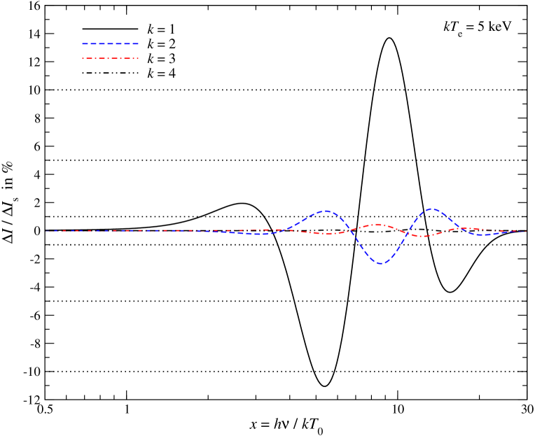
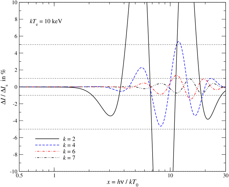
Figure 1: Deviation of the approximation from the numerical result. The asymptotic expansion is used to represent the SZ signal. For each of the curves, k+1𝑘1k+1 temperature orders were included. The departure is expressed in units of ΔIs0.013MJysr1similar-to-or-equalsΔsubscript𝐼s0.013MJysuperscriptsr1\Delta I_{\rm s}\simeq 0.013\,{\rm MJy\,sr^{-1}} and τ=0.01𝜏0.01\tau=0.01 was assumed.
Refer to caption
Refer to caption
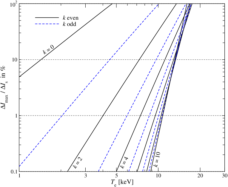
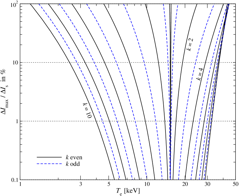
Figure 2: Range of convergence for different approximations. The upper panel shows the results obtained with the asymptotic expansion, while for the lower panel the basis CNSN with θe,0=0.03subscript𝜃e00.03\theta_{\rm e,0}=0.03 was used. The maximal departure for 0.1x300.1𝑥300.1\leq x\leq 30 is expressed in units of ΔIs0.013MJysr1similar-to-or-equalsΔsubscript𝐼s0.013MJysuperscriptsr1\Delta I_{\rm s}\simeq 0.013\,{\rm MJy\,sr^{-1}} and τ=0.01𝜏0.01\tau=0.01 was assumed for all cases.

2.4 Minimizing the required number of moments

One of the important questions is how many moments are needed to describe the SZ signal accurately for a given experimental sensitivity and range of gas temperatures. Here it is particularly interesting to try minimizing the total number of moments that are required to achieve an optimal representation of the SZ signal. To answer this question we first define a fiducial sensitivity for comparison. We shall use the kSZ signal of a cluster with line-of-sight optical depth τ=102𝜏superscript102\tau=10^{-2} and βcμc=103subscript𝛽csubscript𝜇csuperscript103\beta_{\rm c}\mu_{\rm c}=10^{-3} close to the thSZ crossover frequency νc=217GHz(xc=3.83)subscript𝜈c217GHzsubscript𝑥c3.83\nu_{\rm c}=217\,{\rm GHz}\,(x_{\rm c}=3.83) as benchmark; this gives a distortion with amplitude ΔIs9.76τβcμc(kT0)3/[h2c2]sr10.013MJysr1similar-to-or-equalsΔsubscript𝐼s9.76𝜏subscript𝛽csubscript𝜇csuperscript𝑘subscript𝑇03delimited-[]superscript2superscript𝑐2superscriptsr1similar-to-or-equals0.013MJysuperscriptsr1\Delta I_{\rm s}\simeq 9.76\,\tau\,\beta_{\rm c}\mu_{\rm c}(kT_{0})^{3}/[h^{2}c^{2}]\,{\rm sr^{-1}}\simeq 0.013\,{\rm MJy\,sr^{-1}}. For an isothermal cluster with kTe5keVsimilar-to-or-equals𝑘subscript𝑇e5keVkT_{\rm e}\simeq 5\,{\rm keV} electrons and τ=102𝜏superscript102\tau=10^{-2} the maximal thSZ signal is roughly ΔIth0.17MJysr1similar-to-or-equalsΔsubscript𝐼th0.17MJysuperscriptsr1\Delta I_{\rm th}\simeq 0.17\,{\rm MJy\,sr^{-1}} at x6.7similar-to-or-equals𝑥6.7x\simeq 6.7. Therefore, ΔIsΔsubscript𝐼s\Delta I_{\rm s} corresponds to 8%similar-to-or-equalsabsentpercent8\simeq 8\% precision on ΔIthΔsubscript𝐼th\Delta I_{\rm th}.

Before carrying out additional computations we extended the basis of CNSN with additional pivot points (at θe,0=0.01subscript𝜃e00.01\theta_{\rm e,0}=0.01 and 0.10.10.1) such that the SZ signal can be represented in a wider range of temperatures. We provide this basis both in the cluster rest frame and the CMB frame. With the current version of SZpack a 0.001%similar-to-or-equalsabsentpercent0.001\simeq 0.001\% precision is achieved at frequencies 0.01x30less-than-or-similar-to0.01𝑥less-than-or-similar-to300.01\lesssim x\lesssim 30, temperatures kTe75keVless-than-or-similar-to𝑘subscript𝑇e75keVkT_{\rm e}\lesssim 75\,{\rm keV}, and for βc0.01less-than-or-similar-tosubscript𝛽c0.01\beta_{\rm c}\lesssim 0.01 basically at no additional computational cost. We furthermore included the necessary database directly into SZpack such that no time is consumed loading data. In the current implementation evaluation of the SZ signal at 400 frequencies takes about 0.01 seconds on a standard laptop. These routines can also be directly invoked from Python.

One can now calculate how accurately the different sets of basis functions describe the SZ signal for varying kmaxsubscript𝑘maxk_{\rm max}. For the asymptotic expansion we show two examples in Fig. 1. At low temperatures (upper panel) only a few terms in the expansion are needed to achieve a very accurate representation of the SZ signal. The mismatch is usually largest at high frequencies, x10similar-to-or-equals𝑥10x\simeq 10, while below the crossover frequency higher order temperature terms are small, even for larger electron temperatures. The lower panel of Fig. 1 indicates that at higher temperatures the convergence of the asymptotic expansion becomes slower, a problem that is well-known from previous analysis (e.g., see Itoh et al., 1998).

A simple calculation can be used to further quantify the convergence rate of the different basis functions: for a given order in temperature we compute the maximal deviation of the approximation from the numerical result in the frequency range 0.1x300.1𝑥300.1\leq x\leq 30. For both the asymptotic expansion and the basis CNSN with reference temperature θe,0=0.03subscript𝜃e00.03\theta_{\rm e,0}=0.03 the results are shown in Fig. 2. One can see that for the asymptotic expansion the agreement with the numerical result does not improve above kTe13keVsimilar-to-or-equals𝑘subscript𝑇e13keVkT_{\rm e}\simeq 13\,{\rm keV}. At higher temperatures the expansion of CNSN performs much better. In particular, the convergence radius increases strongly when including the first few temperature corrections. One can also observe that for the CNSN basis functions with pivot temperature θe,0=0.03subscript𝜃e00.03\theta_{\rm e,0}=0.03 convergence above kTe40keVsimilar-to-or-equals𝑘subscript𝑇e40keVkT_{\rm e}\simeq 40\,{\rm keV} is not achieved. However, this can be overcome by adding another set of basis functions with pivot θe,0>0.03subscript𝜃e00.03\theta_{\rm e,0}>0.03. For fixed temperature correction order, kmaxsubscript𝑘maxk_{\rm max}, one can therefore try to find an optimal combination of pivot temperatures to cover a large range of temperatures. This is not the absolute minimum with respect to the number of moments, but optimization in this way still is beneficial while remaining sufficiently simple.

Table 1: Optimal distribution of temperature pivots, Te,0isubscriptsuperscript𝑇𝑖e0T^{i}_{\rm e,0}, and regions, [0,Te,low]0subscript𝑇elow[0,T_{\rm e,low}], (Te,low,Te,highI]subscript𝑇elowsuperscriptsubscript𝑇ehighI(T_{\rm e,low},T_{\rm e,high}^{\rm I}], (Te,highI,Te,highII]superscriptsubscript𝑇ehighIsuperscriptsubscript𝑇ehighII(T_{\rm e,high}^{\rm I},T_{\rm e,high}^{\rm II}], etc, for given accuracy goal, ΔI/ΔIsΔ𝐼Δsubscript𝐼s\Delta I/\Delta I_{\rm s}. At temperature TeTe,lowsubscript𝑇esubscript𝑇elowT_{\rm e}\leq T_{\rm e,low} the asymptotic expansion is used, while above expressions based on CNSN are applied. As fiducial accuracy value we used ΔIs0.013MJysr1similar-to-or-equalsΔsubscript𝐼s0.013MJysuperscriptsr1\Delta I_{\rm s}\simeq 0.013\,{\rm MJy\,sr^{-1}} and optical depth τ=0.01𝜏0.01\tau=0.01. Numbers marked with asterisk are only estimated upper bounds, although the approximation is much better. The number of temperature correction terms in each region is kmaxsubscript𝑘maxk_{\rm max}, while ktotsubscript𝑘totk_{\rm tot} gives the total number of temperature terms for all regions. The required number of temperature-velocity moments depends on the settings for kinematic corrections and is not further specified here.
ΔI/ΔIsΔ𝐼Δsubscript𝐼s\Delta I/\Delta I_{\rm s} kmax/ktotsubscript𝑘maxsubscript𝑘totk_{\rm max}/k_{\rm tot} Te,lowsubscript𝑇elowT_{\rm e,low} Te,highI/Te,0Isuperscriptsubscript𝑇ehighIsubscriptsuperscript𝑇Ie0T_{\rm e,high}^{\rm I}/T^{\rm I}_{\rm e,0} Te,highII/Te,0IIsuperscriptsubscript𝑇ehighIIsubscriptsuperscript𝑇IIe0T_{\rm e,high}^{\rm II}/T^{\rm II}_{\rm e,0} Te,highIII/Te,0IIIsuperscriptsubscript𝑇ehighIIIsubscriptsuperscript𝑇IIIe0T_{\rm e,high}^{\rm III}/T^{\rm III}_{\rm e,0}
[keV]delimited-[]keV[\rm keV] [keV]delimited-[]keV[\rm keV] [keV]delimited-[]keV[\rm keV] [keV]delimited-[]keV[\rm keV]
1 2/12 9.1 21.6/1421.61421.6/14 42/30423042/30 75/55755575/55
1 3/12 12.5 48.5/2548.52548.5/25 90/80superscript908090^{\ast}/80
1 4/10 14.3 75/35753575/35
0.1 3/16 6.8 17.25/1117.251117.25/11 36.4/2536.42536.4/25 68/50685068/50
0.1 4/15 9.3 33.1/18.533.118.533.1/18.5 80/55superscript805580^{\ast}/55
0.1 5/18 10.76 48.5/2548.52548.5/25 90/80superscript908090^{\ast}/80
0.01 4/20 5.76 14.7/9.414.79.414.7/9.4 32/22322232/22 61/45614561/45
0.01 5/18 7.3 23.86/1423.861423.86/14 61/40614061/40
0.01 6/21 8.55 33.3/18.533.318.533.3/18.5 80/60superscript806080^{\ast}/60
5×1045superscript1045\times 10^{-4} 6/28 5.76 14.7/9.414.79.414.7/9.4 32/22322232/22 63.5/4563.54563.5/45

In Table 1 we summarize the results of our efforts to cover at least the temperature range 0kTe60keV0𝑘subscript𝑇eless-than-or-similar-to60keV0\leq kT_{\rm e}\lesssim 60\,{\rm keV} for a given precision and kmaxsubscript𝑘maxk_{\rm max}. We defined different regions of temperatures making sure that close to the boundaries the condition on the precision is met with some 10%20%percent10percent2010\%-20\% margin. Far away from the boundaries of the different temperature regions the approximations are typically much more accurate. The setting for accuracy goal 5×10⁴ΔIs5superscript104Δsubscript𝐼s5\times 10^{-4}\Delta I_{\rm s} is already close to the numerical precision of our approximations and is mainly meant to provide an extreme setting for comparisons. Furthermore, if the electron temperature is smaller than some maximal temperature, Te,maxsubscript𝑇emaxT_{\rm e,max}, the total number of required variables can be further reduced by dropping moments in regions with Te>Te,maxsubscript𝑇esubscript𝑇emaxT_{\rm e}>T_{\rm e,max}. For a given accuracy goal this defines an optimal value for kmaxsubscript𝑘maxk_{\rm max}. We also found that the same settings work when 0βc0.01less-than-or-similar-to0subscript𝛽cless-than-or-similar-to0.010\lesssim\beta_{\rm c}\lesssim 0.01.

One point we mention is that the settings given in Table 1 are in fact independent of the chosen optical depth, τ𝜏\tau. This means that only the scaling of the approximation with electron temperature affects the precision. For instance, if the optical depth along a given line-of-sight is τ2×10³similar-to-or-equals𝜏2superscript103\tau\simeq 2\times 10^{-3}, but the temperature is fixed, then the absolute precision of the approximation at accuracy goal in the second category (denoted with 0.1ΔIs0.1Δsubscript𝐼s0.1\Delta I_{\rm s}) is actually 0.02ΔIsless-than-or-similar-toabsent0.02Δsubscript𝐼s\lesssim 0.02\Delta I_{\rm s}.

3 SZ signals for various cluster models

To demonstrate how to use and interpret the temperature-velocity moment method we now discuss the SZ signals for different cluster models. We start with the simplest case of an isothermal cluster and then work our way through several instructive examples, also introducing the simpler moment method that is applicable to sufficiently smooth (low temperature-velocity variance) cluster atmospheres.

3.1 SZ signals for isothermal clusters

Traditionally, galaxy clusters have been modelled using a simple isothermal β𝛽\beta-model (Cavaliere & Fusco-Femiano, 1978):

Nesubscript𝑁e\displaystyle N_{\rm e} =Ne,0[1+(r/rc)2]3β/2andTeconst,formulae-sequenceabsentsubscript𝑁e0superscriptdelimited-[]1superscript𝑟subscript𝑟c23𝛽2andsubscript𝑇econst\displaystyle=N_{\rm e,0}[1+(r/r_{\rm c})^{2}]^{-3\beta/2}\quad{\rm and}\quad T_{\rm e}\equiv{\rm const}, (14)

where Ne,0103cm3similar-to-or-equalssubscript𝑁e0superscript103superscriptcm3N_{\rm e,0}\simeq 10^{-3}{\rm cm^{-3}} is the typical central number density of free electrons, rc100kpcsimilar-to-or-equalssubscript𝑟c100kpcr_{\rm c}\simeq 100\,{\rm kpc} is the typical core radius of clusters, and β2/3similar-to-or-equals𝛽23\beta\simeq 2/3 (e.g., see Reese et al., 2002). In the absence of bulk velocities, one therefore has the temperature moments y(k)=θek+1τsuperscript𝑦𝑘superscriptsubscript𝜃e𝑘1𝜏y^{(k)}=\theta_{\rm e}^{k+1}\tau for TeTe,lowsubscript𝑇esubscript𝑇elowT_{\rm e}\leq T_{\rm e,low} and z(k)=𝒩(θe)θekτsuperscript𝑧𝑘𝒩subscript𝜃esuperscriptsubscript𝜃e𝑘𝜏z^{(k)}=\mathcal{N}(\theta_{\rm e})\,\theta_{\rm e}^{k}\tau for Te>Te,lowsubscript𝑇esubscript𝑇elowT_{\rm e}>T_{\rm e,low}. This shows that the spatial morphology of the SZ signal is fully determined by the overall optical depth factor, τ(𝜸^)𝜏^𝜸\tau({\hat{\boldsymbol{\gamma}}}) (we shall ignore small corrections caused by multiple scattering, e.g., see Dolgov et al., 2001; Itoh et al., 2001; Colafrancesco et al., 2003), with the same spectral shape for any line-of-sight through the cluster. This also implies that the average SZ signal measured for an unresolved cluster in this case is determined by only one spectral function, and the spatially averaged optical depth, τdelimited-⟨⟩𝜏\left<\tau\right>.

Allowing the cluster to move with a peculiar velocity, 𝜷csubscript𝜷c{{\boldsymbol{\beta}}_{\rm c}}, relative to the CMB one readily obtains the velocity moments777We neglected tiny corrections caused by deviations from the flat-sky approximation (Chluba et al., 2012). b0(k)=βc2θekτsubscriptsuperscript𝑏𝑘0superscriptsubscript𝛽c2superscriptsubscript𝜃e𝑘𝜏b^{(k)}_{0}=\beta_{\rm c}^{2}\theta_{\rm e}^{k}\tau, b1(k)βcμcθekτsubscriptsuperscript𝑏𝑘1subscript𝛽csubscript𝜇csuperscriptsubscript𝜃e𝑘𝜏b^{(k)}_{1}\approx\beta_{\rm c}\mu_{\rm c}\theta_{\rm e}^{k}\tau and b2(k)βc2P2(μc)θekτsubscriptsuperscript𝑏𝑘2superscriptsubscript𝛽c2subscript𝑃2subscript𝜇csuperscriptsubscript𝜃e𝑘𝜏b^{(k)}_{2}\approx\beta_{\rm c}^{2}P_{2}(\mu_{\rm c})\theta_{\rm e}^{k}\tau for clusters with TeTe,lowsubscript𝑇esubscript𝑇elowT_{\rm e}\leq T_{\rm e,low}, and c0(k)=βc2𝒩(θe)θekτsubscriptsuperscript𝑐𝑘0superscriptsubscript𝛽c2𝒩subscript𝜃esuperscriptsubscript𝜃e𝑘𝜏c^{(k)}_{0}=\beta_{\rm c}^{2}\mathcal{N}(\theta_{\rm e})\,\theta_{\rm e}^{k}\tau, c1(k)βcμc𝒩(θe)θekτsubscriptsuperscript𝑐𝑘1subscript𝛽csubscript𝜇c𝒩subscript𝜃esuperscriptsubscript𝜃e𝑘𝜏c^{(k)}_{1}\approx\beta_{\rm c}\mu_{\rm c}\mathcal{N}(\theta_{\rm e})\,\theta_{\rm e}^{k}\tau, and c2(k)βc2P2(μc)𝒩(θe)θekτsubscriptsuperscript𝑐𝑘2superscriptsubscript𝛽c2subscript𝑃2subscript𝜇c𝒩subscript𝜃esuperscriptsubscript𝜃e𝑘𝜏c^{(k)}_{2}\approx\beta_{\rm c}^{2}P_{2}(\mu_{\rm c})\mathcal{N}(\theta_{\rm e})\,\theta_{\rm e}^{k}\tau for hot clusters. Again the spatial dependence of the SZ signal factors out and is determined by the one of the line-of-sight optical depth alone. It is however clear that the SZ morphology becomes frequency-dependent888Here we mean that the spectral dependence of the SZ signal no longer is independent of the line-of-sight. once the cluster no longer is isothermal or significant internal motions of the ICM are present. The reason for this frequency-dependence is related to the variation of the temperature-velocity moments along different lines-of-sight, as we illustrate below (Sect. 3.4).

3.2 SZ signals for smooth density and temperature profiles

In more realistic cluster models, the variation of the temperature also has to be included. One common possibility assumes a polytropic temperature profile, Teρgas1γproportional-tosubscript𝑇esuperscriptsubscript𝜌gas1𝛾T_{\rm e}\propto\rho_{\rm gas}^{1-\gamma} (Markevitch et al., 1999; Finoguenov et al., 2001; Pratt & Arnaud, 2002). Alternatively, one can consider fits to the observed temperature and density profiles derived from Chandra X-ray data (Vikhlinin et al., 2006).

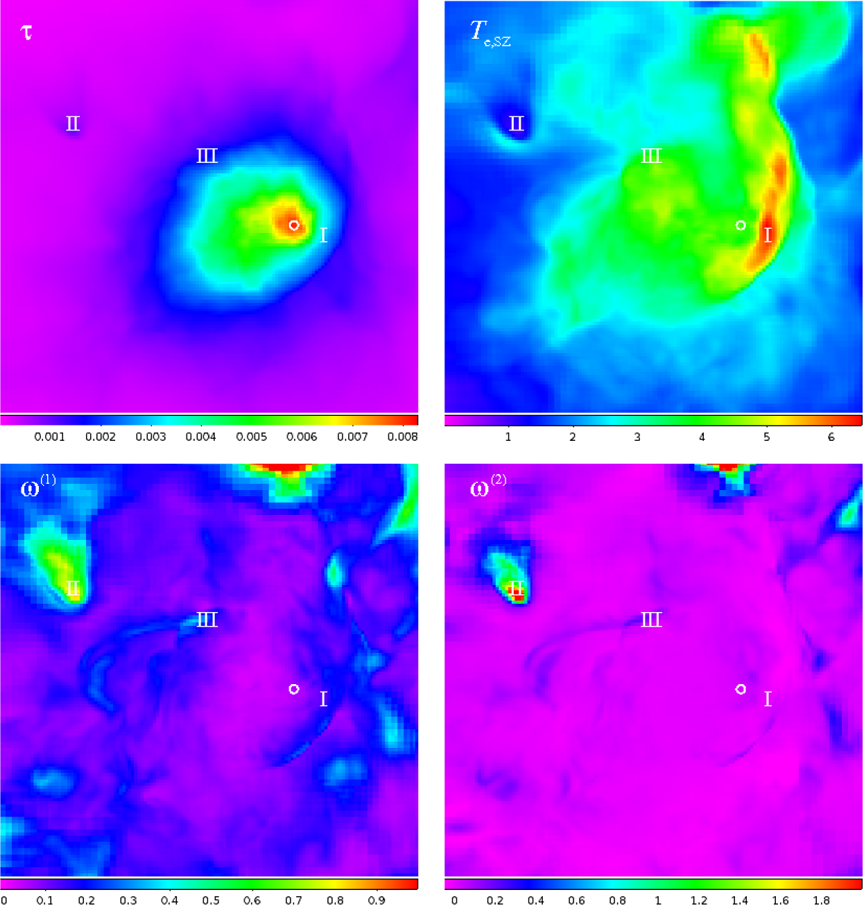
For our discussion it is only important that the associated profiles are very smooth. This suggests that a good approximation for the SZ signal can be found by computing average values for the temperature and velocity along the line-of-sight. Corrections to this lowest order approximation can then be included using a Taylor-series around the average values. Assuming that βc=0subscript𝛽c0\beta_{\rm c}=0, we can introduce the SZ-weighted electron temperature,

Te,SZ(𝜸^)subscript𝑇eSZ^𝜸\displaystyle T_{\rm e,SZ}({\hat{\boldsymbol{\gamma}}}) =(mec2/k)y(0)/y(1)=τ1Tedτ.absentsubscript𝑚esuperscript𝑐2𝑘superscript𝑦0superscript𝑦1superscript𝜏1subscript𝑇edifferential-d𝜏\displaystyle=(m_{\rm e}c^{2}/k)\,y^{(0)}/y^{(-1)}=\tau^{-1}\!\int T_{\rm e}{\,\rm d}\tau. (15)

The integrals y(k)superscript𝑦𝑘y^{(k)} are defined by Eq. (3) but here we do not impose any condition on the electron temperature. One can furthermore introduce the isothermal temperature moments

yiso(k)(𝜸^)=[kTe,SZ(𝜸^)/mec2]k+1τ(𝜸^).superscriptsubscript𝑦iso𝑘^𝜸superscriptdelimited-[]𝑘subscript𝑇eSZ^𝜸subscript𝑚esuperscript𝑐2𝑘1𝜏^𝜸\displaystyle y_{\rm iso}^{(k)}({\hat{\boldsymbol{\gamma}}})=[kT_{\rm e,SZ}({\hat{\boldsymbol{\gamma}}})/m_{\rm e}c^{2}]^{k+1}\,\tau({\hat{\boldsymbol{\gamma}}}). (16)

In general these moments are not identical to y(k)(𝜸^)superscript𝑦𝑘^𝜸y^{(k)}({\hat{\boldsymbol{\gamma}}}) for k>0𝑘0k>0, and the ratio ρ(k)(𝜸^)=y(k)/yiso(k)τky(k)/[y(0)]k+1superscript𝜌𝑘^𝜸superscript𝑦𝑘superscriptsubscript𝑦iso𝑘superscript𝜏𝑘superscript𝑦𝑘superscriptdelimited-[]superscript𝑦0𝑘1\rho^{(k)}({\hat{\boldsymbol{\gamma}}})=y^{(k)}/y_{\rm iso}^{(k)}\equiv\tau^{k}y^{(k)}/[y^{(0)}]^{k+1} can be used to quantify departures from isothermality: in regions with ρ(k)1superscript𝜌𝑘1\rho^{(k)}\neq 1 one expects the SZ signal to be poorly represented by just using the SZ-weighted electron temperature and line-of-sight optical depth. The ratios ρ(k)superscript𝜌𝑘\rho^{(k)} are also independent of the overall temperature and density scales. They only depend on the shapes of the cluster temperature and electron density profiles.

We can write this more formally by using the isothermal moment vector, 𝒎iso(τ,Te,SZ)subscript𝒎iso𝜏subscript𝑇eSZ\mbox{\boldmath${m}$\unboldmath}_{\rm iso}(\tau,T_{\rm e,SZ}), and expanding the average SZ signal around Te,SZsubscript𝑇eSZT_{\rm e,SZ} and τ𝜏\tau:

𝑺𝑺{S} 𝗙[𝒎iso(τ,Te,SZ)+k=2kmaxθe,SZk𝒎iso(Te,SZ)τk!(θeθe,SZ)kdτ]absent𝗙delimited-[]subscript𝒎iso𝜏subscript𝑇eSZsuperscriptsubscript𝑘2subscript𝑘maxsubscriptsuperscript𝑘subscript𝜃eSZsubscript𝒎isosubscript𝑇eSZ𝜏𝑘superscriptsubscript𝜃esubscript𝜃eSZ𝑘differential-d𝜏\displaystyle\approx\boldsymbol{\mathsf{F}}\,\left[\mbox{\boldmath${m}$\unboldmath}_{\rm iso}(\tau,T_{\rm e,SZ})+\sum_{k=2}^{k_{\rm max}}\frac{\partial^{k}_{\theta_{\rm e,SZ}}\mbox{\boldmath${m}$\unboldmath}_{\rm iso}(T_{\rm e,SZ})}{\tau\,k!}\int(\theta_{\rm e}-\theta_{\rm e,SZ})^{k}{\,\rm d}\tau\right]

where the first order derivative term canceled after performing the line-of-sight average. Here 𝑺iso(τ,Te,SZ)=𝗙𝒎iso(τ,Te,SZ)subscript𝑺iso𝜏subscript𝑇eSZ𝗙subscript𝒎iso𝜏subscript𝑇eSZ\mbox{\boldmath${S}$\unboldmath}_{\rm iso}(\tau,T_{\rm e,SZ})=\boldsymbol{\mathsf{F}}\,\mbox{\boldmath${m}$\unboldmath}_{\rm iso}(\tau,T_{\rm e,SZ}) is the leading order, average SZ signal, while θek𝑺iso(Te)=𝗙θek𝒎iso(Te)subscriptsuperscript𝑘subscript𝜃esubscript𝑺isosubscript𝑇e𝗙subscriptsuperscript𝑘subscript𝜃esubscript𝒎isosubscript𝑇e\partial^{k}_{\theta_{\rm e}}\mbox{\boldmath${S}$\unboldmath}_{\rm iso}(T_{\rm e})=\boldsymbol{\mathsf{F}}\,\partial^{k}_{\theta_{\rm e}}\mbox{\boldmath${m}$\unboldmath}_{\rm iso}(T_{\rm e}) is the derivatives of the SZ signal with respect to θesubscript𝜃e\theta_{\rm e}. To simplify the notation, we furthermore introduce

Δy(k)Δsuperscript𝑦𝑘\displaystyle\Delta y^{(k)} =(θeθe,SZ)k+1dτ=yiso(k)m=0k+1(k+1m)(1)k+1mρ(m1).absentsuperscriptsubscript𝜃esubscript𝜃eSZ𝑘1differential-d𝜏subscriptsuperscript𝑦𝑘isosuperscriptsubscript𝑚0𝑘1binomial𝑘1𝑚superscript1𝑘1𝑚superscript𝜌𝑚1\displaystyle=\int(\theta_{\rm e}-\theta_{\rm e,SZ})^{k+1}{\,\rm d}\tau=y^{(k)}_{\rm iso}\sum_{m=0}^{k+1}\binom{k+1}{m}\,(-1)^{k+1-m}\rho^{(m-1)}.

This means Δy(0)=0Δsuperscript𝑦00\Delta y^{(0)}=0, Δy(1)=y(1)yiso(1)=yiso(1)Δρ(1)Δsuperscript𝑦1superscript𝑦1subscriptsuperscript𝑦1isosubscriptsuperscript𝑦1isoΔsuperscript𝜌1\Delta y^{(1)}=y^{(1)}-y^{(1)}_{\rm iso}=y^{(1)}_{\rm iso}\,\Delta\rho^{(1)}, Δy(2)=yiso(2)Δρ(2)3yiso(2)Δρ(1)Δsuperscript𝑦2subscriptsuperscript𝑦2isoΔsuperscript𝜌23subscriptsuperscript𝑦2isoΔsuperscript𝜌1\Delta y^{(2)}=y^{(2)}_{\rm iso}\,\Delta\rho^{(2)}-3y^{(2)}_{\rm iso}\,\Delta\rho^{(1)}, and so on, with Δρ(k)=ρ(k)1Δsuperscript𝜌𝑘superscript𝜌𝑘1\Delta\rho^{(k)}=\rho^{(k)}-1. Defining ω(k)=Δy(k)/yiso(k)τkΔy(k)/[y(0)]k+1superscript𝜔𝑘Δsuperscript𝑦𝑘subscriptsuperscript𝑦𝑘isosuperscript𝜏𝑘Δsuperscript𝑦𝑘superscriptdelimited-[]superscript𝑦0𝑘1\omega^{(k)}=\Delta y^{(k)}/y^{(k)}_{\rm iso}\equiv\tau^{k}\Delta y^{(k)}/[y^{(0)}]^{k+1} we then can finally write

𝑺𝑺{S} 𝑺iso(0)(τ,Te,SZ)+𝑺iso(2)(τ,Te,SZ)ω(1)+𝑺iso(3)(τ,Te,SZ)ω(2)+absentsubscriptsuperscript𝑺0iso𝜏subscript𝑇eSZsubscriptsuperscript𝑺2iso𝜏subscript𝑇eSZsuperscript𝜔1subscriptsuperscript𝑺3iso𝜏subscript𝑇eSZsuperscript𝜔2\displaystyle\approx\mbox{\boldmath${S}$\unboldmath}^{(0)}_{\rm iso}(\tau,T_{\rm e,SZ})+\mbox{\boldmath${S}$\unboldmath}^{(2)}_{\rm iso}(\tau,T_{\rm e,SZ})\,\omega^{(1)}+\mbox{\boldmath${S}$\unboldmath}^{(3)}_{\rm iso}(\tau,T_{\rm e,SZ})\,\omega^{(2)}+... (17)

where 𝑺iso(k)(τ,T)=(Tk/k!)Tk𝑺iso(τ,T)subscriptsuperscript𝑺𝑘iso𝜏𝑇superscript𝑇𝑘𝑘subscriptsuperscript𝑘𝑇subscript𝑺iso𝜏𝑇\mbox{\boldmath${S}$\unboldmath}^{(k)}_{\rm iso}(\tau,T)=(T^{k}/k!)\,\partial^{k}_{T}\mbox{\boldmath${S}$\unboldmath}_{\rm iso}(\tau,T). In this parametrization the observables for the SZ measurement are τ𝜏\tau, Te,SZsubscript𝑇eSZT_{\rm e,SZ}, and the temperature moments ω(k)superscript𝜔𝑘\omega^{(k)}.

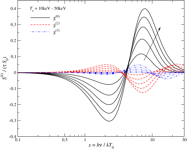
With SZpack it is straightforward to compute the required vectors, 𝑺iso(k)subscriptsuperscript𝑺𝑘iso\mbox{\boldmath${S}$\unboldmath}^{(k)}_{\rm iso}, with very high precision. In Fig. 3 we show the first few 𝑺iso(k)subscriptsuperscript𝑺𝑘iso\mbox{\boldmath${S}$\unboldmath}^{(k)}_{\rm iso}.

Refer to caption
Figure 3: Spectral functions 𝑺iso(k)subscriptsuperscript𝑺𝑘iso\mbox{\boldmath${S}$\unboldmath}^{(k)}_{\rm iso} in units of τ𝜏\tau and S0=(2h/c2)(kT0/h)3270MJysr1subscript𝑆02superscript𝑐2superscript𝑘subscript𝑇03270MJysuperscriptsr1S_{0}=(2h/c^{2})(kT_{0}/h)^{3}\approx 270\,{\rm MJy\,sr^{-1}}. For comparison we also show the main SZ signal (solid black line). The arrow indicates the direction of increasing temperature, with the lines within the groups being separated by ΔTe=10keVΔsubscript𝑇e10keV\Delta T_{\rm e}=10\,{\rm keV}.

The typical amplitude of the 𝑺iso(k)subscriptsuperscript𝑺𝑘iso\mbox{\boldmath${S}$\unboldmath}^{(k)}_{\rm iso} is dropping with k𝑘k, indicating that unless the temperature moments ω(k)superscript𝜔𝑘\omega^{(k)} increase strongly with k𝑘k, higher order terms remain small with the largest contributions at high frequencies. This shows that the considered expansion becomes fully perturbative unless rather large deviations from the smooth temperature profile case are present.

For example, using the simple fits for one of the hottest clusters (Te9.2keVsimilar-to-or-equalssubscript𝑇e9.2keVT_{\rm e}\simeq 9.2\,{\rm keV} at r330kpcsimilar-to-or-equals𝑟330kpcr\simeq 330\,{\rm kpc}), A2029, from the cluster sample of Vikhlinin et al. (2006), we find ω(1)0.16similar-to-or-equalssuperscript𝜔10.16\omega^{(1)}\simeq 0.16, ω(2)0similar-to-or-equalssuperscript𝜔20\omega^{(2)}\simeq 0, and ω(3)0.05similar-to-or-equalssuperscript𝜔30.05\omega^{(3)}\simeq 0.05 close to the cluster center. This indicates that higher order corrections decay rapidly. In fact, the correction related to ω(1)superscript𝜔1\omega^{(1)} contributes at the level of a few percent to the average SZ signal, while higher order moments are negligible. We find that even for more realistic cases from simulated clusters only a few moments of the temperature field need to be known to accurately describe the SZ signal (Sect. 3.4). Also, in the more extreme case of a two-temperature plasma only the first few terms are required (Sect. 3.3).

Some interesting frequencies for the functions 𝑺iso(k)subscriptsuperscript𝑺𝑘iso\mbox{\boldmath${S}$\unboldmath}^{(k)}_{\rm iso} are related to their nulls, maxima and minima. For 𝑺iso(1)subscriptsuperscript𝑺1iso\mbox{\boldmath${S}$\unboldmath}^{(1)}_{\rm iso} (which is not shown in Fig. 3) we find a rather temperature-independent minimum at x2.26similar-to-or-equals𝑥2.26x\simeq 2.26. At x4similar-to-or-equals𝑥4x\simeq 4 it crosses zero for Te10keVsimilar-to-or-equalssubscript𝑇e10keVT_{\rm e}\simeq 10\,{\rm keV}, while for Te50keVsimilar-to-or-equalssubscript𝑇e50keVT_{\rm e}\simeq 50\,{\rm keV} the null is located at x4.89similar-to-or-equals𝑥4.89x\simeq 4.89. Its maximum is located at x7.2similar-to-or-equals𝑥7.2x\simeq 7.2 for Te=10keVsubscript𝑇e10keVT_{\rm e}=10\,{\rm keV} and at x10similar-to-or-equals𝑥10x\simeq 10 for Te=50keVsubscript𝑇e50keVT_{\rm e}=50\,{\rm keV}. For 𝑺iso(2)subscriptsuperscript𝑺2iso\mbox{\boldmath${S}$\unboldmath}^{(2)}_{\rm iso} (see Fig. 3) on the other hand we find a maximum at x2.12similar-to-or-equals𝑥2.12x\simeq 2.12 and the first null at x3.5similar-to-or-equals𝑥3.5x\simeq 3.5. The position of the minimum varies from x5.8similar-to-or-equals𝑥5.8x\simeq 5.8 for Te=10keVsubscript𝑇e10keVT_{\rm e}=10\,{\rm keV} to x7.2similar-to-or-equals𝑥7.2x\simeq 7.2 for Te=50keVsubscript𝑇e50keVT_{\rm e}=50\,{\rm keV}. These properties might be useful when deciding about the locations of frequency channels in future SZ experiments.

We emphasize that for the computation of 𝑺iso(0)(τ,Te,SZ)subscriptsuperscript𝑺0iso𝜏subscript𝑇eSZ\mbox{\boldmath${S}$\unboldmath}^{(0)}_{\rm iso}(\tau,T_{\rm e,SZ}) and 𝑺iso(2)(τ,Te,SZ)subscriptsuperscript𝑺2iso𝜏subscript𝑇eSZ\mbox{\boldmath${S}$\unboldmath}^{(2)}_{\rm iso}(\tau,T_{\rm e,SZ}) a large number of temperature terms has to be included. Although in the example given above we only find ω(1)superscript𝜔1\omega^{(1)} to be significant as additional parameter, this is not equivalent to dropping higher order temperature terms. This point is very important when interpreting future SZ data, since otherwise biased results for τ,Te,SZ𝜏subscript𝑇eSZ\tau,T_{\rm e,SZ}, and ω(1)superscript𝜔1\omega^{(1)} are obtained. Similarly, one has to include βcμc0subscript𝛽csubscript𝜇c0\beta_{\rm c}\mu_{\rm c}\neq 0 for the analysis, as we discuss in more detail below.

We also note that Eq. (17) is applicable even if the real temperature distribution is not a smooth function. It is only important that the variance of the temperature and thermal pressure remains sufficiently low to warrant decreasing values of the moments, ω(k)superscript𝜔𝑘\omega^{(k)}, with larger k𝑘k. This condition is usually fulfilled even in more realistic cluster models (see Sect. 3.4).

3.2.1 The effect of line-of-sight temperature variance

Above we showed that the dominant correction to the SZ signal is determined by the temperature moment ω(1)superscript𝜔1\omega^{(1)}. This parameter can be interpreted as line-of-sight variance or dispersion of the electron temperature but weighted by the optical depth of the scattering volume element. One can now address the question of how important this term is for the interpretation of the SZ signal. In particular, by how much are the deduced best-fit values for Te,SZsubscript𝑇eSZT_{\rm e,SZ} and τ𝜏\tau affected if the contribution from ω(1)superscript𝜔1\omega^{(1)} is neglected for high-sensitivity, multi-frequency SZ measurements.

We can start by writing the SZ signal for Te,SZTe,SZsubscriptsuperscript𝑇eSZsubscript𝑇eSZT^{\ast}_{\rm e,SZ}\neq T_{\rm e,SZ} as an expansion of 𝑺(τ,Te,SZ)𝑺superscript𝜏subscriptsuperscript𝑇eSZ\mbox{\boldmath${S}$\unboldmath}(\tau^{\ast},T^{\ast}_{\rm e,SZ}) around Te,SZsubscript𝑇eSZT_{\rm e,SZ} and τ𝜏\tau:

𝑺(τ,Te,SZ)𝑺superscript𝜏subscriptsuperscript𝑇eSZ\displaystyle\mbox{\boldmath${S}$\unboldmath}(\tau^{\ast},T^{\ast}_{\rm e,SZ}) 𝑺iso(0)(τ,Te,SZ)+𝑺iso(0)(τ,Te,SZ)Θτ+𝑺iso(1)(τ,Te,SZ)Θ,absentsubscriptsuperscript𝑺0iso𝜏subscript𝑇eSZsubscriptsuperscript𝑺0iso𝜏subscript𝑇eSZsubscriptΘ𝜏subscriptsuperscript𝑺1iso𝜏subscript𝑇eSZΘ\displaystyle\approx\mbox{\boldmath${S}$\unboldmath}^{(0)}_{\rm iso}(\tau,T_{\rm e,SZ})+{\mbox{\boldmath${S}$\unboldmath}^{(0)}_{\rm iso}}(\tau,T_{\rm e,SZ})\,\Theta_{\tau}+\mbox{\boldmath${S}$\unboldmath}^{(1)}_{\rm iso}(\tau,T_{\rm e,SZ})\,\Theta,

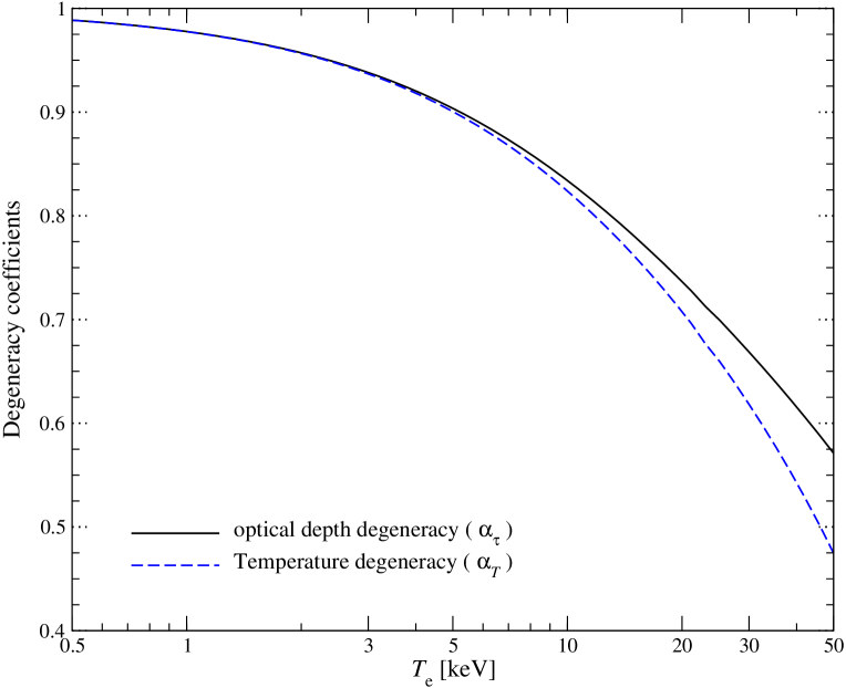
where Θ=(Te,SZTe,SZ)/Te,SZΘsubscriptsuperscript𝑇eSZsubscript𝑇eSZsubscript𝑇eSZ\Theta=(T^{\ast}_{\rm e,SZ}-T_{\rm e,SZ})/T_{\rm e,SZ}, Θτ=(ττ)/τsubscriptΘ𝜏superscript𝜏𝜏𝜏\Theta_{\tau}=(\tau^{\ast}-\tau)/\tau, and we neglected higher order terms. To determine the best-fit values for τsuperscript𝜏\tau^{\ast} and Te,SZsubscriptsuperscript𝑇eSZT^{\ast}_{\rm e,SZ} one has to compare to 𝑺(τ,Te,SZ,ω(1))𝑺iso(0)(τ,Te,SZ)+𝑺iso(2)(τ,Te,SZ)ω(1)𝑺𝜏subscript𝑇eSZsuperscript𝜔1subscriptsuperscript𝑺0iso𝜏subscript𝑇eSZsubscriptsuperscript𝑺2iso𝜏subscript𝑇eSZsuperscript𝜔1\mbox{\boldmath${S}$\unboldmath}(\tau,T_{\rm e,SZ},\omega^{(1)})\approx\mbox{\boldmath${S}$\unboldmath}^{(0)}_{\rm iso}(\tau,T_{\rm e,SZ})+\mbox{\boldmath${S}$\unboldmath}^{(2)}_{\rm iso}(\tau,T_{\rm e,SZ})\,\omega^{(1)} and then minimize the squared difference. The coefficients relating ΘτsubscriptΘ𝜏\Theta_{\tau} and ΘΘ\Theta to ω(1)superscript𝜔1\omega^{(1)} then are only functions of temperature, and it is straightforward to compute the degeneracy coefficients ατ=Θτ/ω(1)subscript𝛼𝜏subscriptΘ𝜏superscript𝜔1\alpha_{\rm\tau}=-\Theta_{\tau}/\omega^{(1)} and αT=Θ/ω(1)subscript𝛼𝑇Θsuperscript𝜔1\alpha_{T}=\Theta/\omega^{(1)} (Fig. 4). Both τ𝜏\tau and Te,SZsubscript𝑇eSZT_{\rm e,SZ} are correlated with ω(1)superscript𝜔1\omega^{(1)} to a similar degree. The degeneracy is very close to unity at low temperatures and only drops to about 1/2121/2 at very high temperatures. We find that ατ(Te)[1+2.7×10²Te0.86]1subscript𝛼𝜏subscript𝑇esuperscriptdelimited-[]12.7superscript102superscriptsubscript𝑇e0.861\alpha_{\tau}(T_{\rm e})\approx[1+2.7\times 10^{-2}\,T_{\rm e}^{0.86}]^{-1} and αTexp(2.6×10²Te0.86)subscript𝛼𝑇2.6superscript102superscriptsubscript𝑇e0.86\alpha_{T}\approx\exp\left(-2.6\times 10^{-2}\,T_{\rm e}^{0.86}\right) match the full numerical result with 10%similar-to-or-equalsabsentpercent10\simeq 10\% precision. With these expressions we can directly estimate the expected value for Te,SZsubscriptsuperscript𝑇eSZT^{\ast}_{\rm e,SZ} obtained by computing the best-fits to the full SZ signal.
Refer to caption
Figure 4: Degeneracies of τ𝜏\tau and Te,SZsubscript𝑇eSZT_{\rm e,SZ} with ω(1)superscript𝜔1\omega^{(1)}. The expected (biased) best-fit values are ττ[1ατ(Te)ω(1)]superscript𝜏𝜏delimited-[]1subscript𝛼𝜏subscript𝑇esuperscript𝜔1\tau^{\ast}\approx\tau[1-\alpha_{\tau}(T_{\rm e})\,\omega^{(1)}] and Te,SZTe,SZ[1+αT(Te)ω(1)]superscriptsubscript𝑇eSZsubscript𝑇eSZdelimited-[]1subscript𝛼𝑇subscript𝑇esuperscript𝜔1T_{\rm e,SZ}^{\ast}\approx T_{\rm e,SZ}[1+\alpha_{T}(T_{\rm e})\,\omega^{(1)}] when analyzing the SZ signal.

To determine the degeneracy coefficients we used a very dense grid of frequency points in the range x=0.1𝑥0.1x=0.1 to 303030. More realistically far fewer independent frequency bins are available plus the signal is averaged over some bandwidth and the beam. Furthermore, foregrounds and the experimental sensitivity at each frequency are important. All these aspects affect the degeneracy between the SZ parameters, as we explain in more detail below (Sect. 5.1). Nevertheless, the estimate obtained above gives a rough scaling for the importance of line-of-sight temperature variations for the interpretation of the SZ measurement.

3.2.2 The effect of velocity terms on the SZ signal

Thus far we neglected the effect of bulk velocity on the SZ signal. However, the effect of (internal) motions can again be included by expanding the SZ signal around the mean line-of-sight values. We first define the two velocity components βc,=βcμc\beta_{\rm c,\parallel}=\beta_{\rm c}\mu_{\rm c} and βc,=βc1μc2subscript𝛽cperpendicular-tosubscript𝛽c1superscriptsubscript𝜇c2\beta_{\rm c,\perp}=\beta_{\rm c}\sqrt{1-\mu_{\rm c}^{2}} of the moving volume element. Since we do not consider the effect of polarization these are the only two variables that matter for the SZ signal. At lowest order in βcsubscript𝛽c\beta_{\rm c} one is only sensitive to the line-of-sight SZ weighted averaged velocity βc,,SZ=τ1βc,dτ\beta_{\rm c,\parallel,SZ}=\tau^{-1}\int\beta_{\rm c,\parallel}{\,\rm d}\tau. The associated kSZ signal has a spectral shape that is very different from the thSZ. It is therefore rather easy to distinguish the two. However, the results for the best-fit values of τ𝜏\tau and Te,SZsubscript𝑇eSZT_{\rm e,SZ} can be strongly biased even for a small (βc,103\beta_{\rm c,\parallel}\simeq 10^{-3}) line-of-sight velocity if neglected in the analysis (see Sect. 5.1).

Looking at the total SZ signal, Eq. (2), with βc2=βc,2+βc,2\beta_{\rm c}^{2}=\beta^{2}_{\rm c,\parallel}+\beta^{2}_{\rm c,\perp} and βc2P2(μc)=βc,2βc,2\beta_{\rm c}^{2}P_{2}(\mu_{\rm c})=\beta^{2}_{\rm c,\parallel}-\beta^{2}_{\rm c,\perp}, it is clear that the SZ signal is only sensitive to βc,,SZ2=τ1βc,2dτsubscriptsuperscript𝛽2cperpendicular-toSZsuperscript𝜏1subscriptsuperscript𝛽2cperpendicular-todifferential-d𝜏\beta^{2}_{\rm c,\perp,SZ}=\tau^{-1}\int\beta^{2}_{\rm c,\perp}{\,\rm d}\tau, but not βc,,SZsubscript𝛽cperpendicular-toSZ\beta_{\rm c,\perp,SZ} directly. For simplicity (and because the associated terms are extremely small) we shall neglect the variation of temperature-velocity cross terms of order 𝒪(βc2θek)𝒪superscriptsubscript𝛽c2superscriptsubscript𝜃e𝑘\mathcal{O}(\beta_{\rm c}^{2}\theta_{\rm e}^{k}) in the discussion here. Expanding around τ𝜏\tau, Te,SZsubscript𝑇eSZT_{\rm e,SZ}, βc,,SZ\beta_{\rm c,\parallel,SZ}, and βc,,SZ=0subscript𝛽cperpendicular-toSZ0\beta_{\rm c,\perp,SZ}=0, the average SZ signal takes the form

𝑺𝑺{S} 𝑺iso(0)+𝑺iso(2)ω(1)+𝑪iso(1)σ(1)+𝑫iso(2)κ(1)+𝑬iso(2)βc,,SZ2+,absentsubscriptsuperscript𝑺0isosubscriptsuperscript𝑺2isosuperscript𝜔1subscriptsuperscript𝑪1isosuperscript𝜎1subscriptsuperscript𝑫2isosuperscript𝜅1subscriptsuperscript𝑬2isosubscriptsuperscript𝛽2cperpendicular-toSZ\displaystyle\approx\mbox{\boldmath${S}$\unboldmath}^{(0)}_{\rm iso}+\mbox{\boldmath${S}$\unboldmath}^{(2)}_{\rm iso}\,\omega^{(1)}+\mbox{\boldmath${C}$\unboldmath}^{(1)}_{\rm iso}\,\sigma^{(1)}+\mbox{\boldmath${D}$\unboldmath}^{(2)}_{\rm iso}\,\kappa^{(1)}+\mbox{\boldmath${E}$\unboldmath}^{(2)}_{\rm iso}\,\beta^{2}_{\rm c,\perp,SZ}+..., (18)

where we suppressed the function arguments τ𝜏\tau, Te,SZsubscript𝑇eSZT_{\rm e,SZ}, and βc,,SZ\beta_{\rm c,\parallel,SZ}. We furthermore defined the signal vectors and dispersion variables,

𝑪iso(k)subscriptsuperscript𝑪𝑘iso\displaystyle\mbox{\boldmath${C}$\unboldmath}^{(k)}_{\rm iso} =(k!m!)1θe,SZkθe,SZkβc,,SZ𝑺iso(τ,Te,SZ,βc,,SZ,βc,,SZ)\displaystyle=(k!\,m!)^{-1}\,\theta^{k}_{\rm e,SZ}\partial^{k}_{\theta_{\rm e,SZ}}\partial_{\beta_{\rm c,\parallel,SZ}}\mbox{\boldmath${S}$\unboldmath}_{\rm iso}(\tau,T_{\rm e,SZ},\beta_{\rm c,\parallel,SZ},\beta_{\rm c,\perp,SZ})
𝑫iso(k)subscriptsuperscript𝑫𝑘iso\displaystyle\mbox{\boldmath${D}$\unboldmath}^{(k)}_{\rm iso} =(k!)1βc,,SZk𝑺iso(τ,Te,SZ,βc,,SZ,βc,,SZ)\displaystyle=(k!)^{-1}\,\partial^{k}_{\beta_{\rm c,\parallel,SZ}}\mbox{\boldmath${S}$\unboldmath}_{\rm iso}(\tau,T_{\rm e,SZ},\beta_{\rm c,\parallel,SZ},\beta_{\rm c,\perp,SZ})
𝑬iso(k)subscriptsuperscript𝑬𝑘iso\displaystyle\mbox{\boldmath${E}$\unboldmath}^{(k)}_{\rm iso} =(k!)1βc,,SZk𝑺iso(τ,Te,SZ,βc,,SZ,βc,,SZ)\displaystyle=(k!)^{-1}\,\partial^{k}_{\beta_{\rm c,\perp,SZ}}\mbox{\boldmath${S}$\unboldmath}_{\rm iso}(\tau,T_{\rm e,SZ},\beta_{\rm c,\parallel,SZ},\beta_{\rm c,\perp,SZ})
κ(k)superscript𝜅𝑘\displaystyle\kappa^{(k)} =τ1(βc,βc,,SZ)k+1dτ\displaystyle=\tau^{-1}\int(\beta_{\rm c,\parallel}-\beta_{\rm c,\parallel,SZ})^{k+1}{\,\rm d}\tau
σ(k)superscript𝜎𝑘\displaystyle\sigma^{(k)} =(Te,SZkτ)1(TeTe,SZ)k(βc,βc,,SZ)dτ,\displaystyle=(T^{k}_{\rm e,SZ}\tau)^{-1}\int(T_{\rm e}-T_{\rm e,SZ})^{k}(\beta_{\rm c,\parallel}-\beta_{\rm c,\parallel,SZ}){\,\rm d}\tau, (19)

where the derivatives are evaluated at βc,,SZ=0subscript𝛽cperpendicular-toSZ0\beta_{\rm c,\perp,SZ}=0. Since in general βcsubscript𝛽c\beta_{\rm c} can vanish, we did not rescale the velocity derivative terms, and correspondingly defined the velocity moments without weighting by the mean values.

As we argue below, for future multi-frequency SZ analysis the average SZ signal is described very well by Eq. (18). This implies that the SZ parameter estimation problem for a single lines-of-sight boils down to constraining the set of SZ parameters 𝒑=(τ,Te,SZ,βc,,SZ,ω(1),σ(1),κ(1),βc,,SZ2)\mbox{\boldmath${p}$\unboldmath}=(\tau,T_{\rm e,SZ},\beta_{\rm c,\parallel,SZ},\omega^{(1)},\sigma^{(1)},\kappa^{(1)},\beta^{2}_{\rm c,\perp,SZ}). Here we ordered the parameters according to their expected importance for the average SZ signal. Higher order temperature and velocity moments are straightforward to add to the problem and maps of the deduced quantities then allow constraining the structure of the cluster. Maps of the different components of 𝒑𝒑{p} therefore provide a compressed version of future multi-frequency, high resolution SZ data cubes. These new variables then directly allow constraining properties of the 3-dimensional cluster’s atmosphere.

Refer to caption
Figure 5: Second frequency derivative of thSZ distortion in units of τ𝜏\tau and S0=(2h/c2)(kT0/h)3270MJysr1subscript𝑆02superscript𝑐2superscript𝑘subscript𝑇03270MJysuperscriptsr1S_{0}=(2h/c^{2})(kT_{0}/h)^{3}\approx 270\,{\rm MJy\,sr^{-1}}. The arrow indicates the direction of increasing temperature, with the lines being separated by ΔTe=10keVΔsubscript𝑇e10keV\Delta T_{\rm e}=10\,{\rm keV}.

3.2.3 Effect of angular resolution on the SZ signal

When deducing the best-fit parameters for τ𝜏\tau, Te,SZsubscript𝑇eSZT_{\rm e,SZ}, and βc,,SZ\beta_{\rm c,\parallel,SZ} it is also important to include the effect of angular resolution on the measured SZ signal. Gradients of the temperature and velocity field within the beam affect these values, as we illustrate here.

One can model the beam as a simple 2-dimensional Gaussian with radius, rressubscript𝑟resr_{\rm res}, or a beam variance σb2=rres2/[2ln(2)]0.721rres2superscriptsubscript𝜎b2superscriptsubscript𝑟res2delimited-[]220.721subscriptsuperscript𝑟2res\sigma_{\rm b}^{2}=r_{\rm res}^{2}/[2\ln(2)]\approx 0.721\,r^{2}_{\rm res}. With the moment method described above we simply have to replace 𝒎𝒎{m} with 𝒎delimited-⟨⟩𝒎\left<\mbox{\boldmath${m}$\unboldmath}\right> in Eq. (12), where delimited-⟨⟩\left<...\right> denotes the average over the beam. For a given electron density, temperature and velocity field, the associated 3-dimensional integrals are in principle straightforward to compute. However, in detail this can already be rather demanding, since several integrals have to be evaluated, respecting the conditions for the different temperature regions.

On the other hand, assuming rather smooth cluster profiles and small beam radius the calculation again simplifies significantly. Let the beam be centered on 𝒓0=(rx,0,ry,0)subscript𝒓0subscript𝑟𝑥0subscript𝑟𝑦0\mbox{\boldmath${r}$\unboldmath}_{0}=(r_{x,0},r_{y,0}) with central values τ0subscript𝜏0\tau_{0}, Te,SZ,0subscript𝑇eSZ0T_{\rm e,SZ,0}, and βc,,SZ,0\beta_{\rm c,\parallel,SZ,0}. The average SZ signal around 𝒓0subscript𝒓0\mbox{\boldmath${r}$\unboldmath}_{0} can be computed from Eq. (18) and (3.2.2) by replacing ττ𝜏delimited-⟨⟩𝜏\tau\rightarrow\left<\tau\right>, Te,SZTe,SZsubscript𝑇eSZdelimited-⟨⟩subscript𝑇eSZT_{\rm e,SZ}\rightarrow\left<T_{\rm e,SZ}\right>, and βc,,SZβc,,SZ\beta_{\rm c,\parallel,SZ}\rightarrow\left<\beta_{\rm c,\parallel,SZ}\right>. Furthermore, one has to substitute βc,,SZ2βc,,SZ2βc,,SZ,02subscriptsuperscript𝛽2cperpendicular-toSZdelimited-⟨⟩subscriptsuperscript𝛽2cperpendicular-toSZsubscriptsuperscript𝛽2cperpendicular-toSZ0\beta^{2}_{\rm c,\perp,SZ}\rightarrow\left<\beta^{2}_{\rm c,\perp,SZ}\right>\approx\beta^{2}_{\rm c,\perp,SZ,0} and compute the beam averages of ω(1)superscript𝜔1\omega^{(1)}, σ(1)superscript𝜎1\sigma^{(1)}, and κ(1)superscript𝜅1\kappa^{(1)}, which read:

ω(1)delimited-⟨⟩superscript𝜔1\displaystyle\left<\omega^{(1)}\right> τ1Te,SZ2(TeTe,SZ)2dτabsentsuperscriptdelimited-⟨⟩𝜏1superscriptdelimited-⟨⟩subscript𝑇eSZ2delimited-⟨⟩superscriptsubscript𝑇edelimited-⟨⟩subscript𝑇eSZ2differential-d𝜏\displaystyle\approx\left<\tau\right>^{-1}\,\left<T_{\rm e,SZ}\right>^{-2}\left<\int\left(T_{\rm e}-\left<T_{\rm e,SZ}\right>\right)^{2}{\,\rm d}\tau\right>
κ(1)delimited-⟨⟩superscript𝜅1\displaystyle\left<\kappa^{(1)}\right> τ1(βc,βc,,SZ)2dτ\displaystyle\approx\left<\tau\right>^{-1}\left<\int\left(\beta_{\rm c,\parallel}-\left<\beta_{\rm c,\parallel,SZ}\right>\right)^{2}{\,\rm d}\tau\right> (20)
σ(1)delimited-⟨⟩superscript𝜎1\displaystyle\left<\sigma^{(1)}\right> =τ1Te,SZ1(TeTe,SZ)(βc,βc,,SZ)dτ.\displaystyle=\left<\tau\right>^{-1}\left<T_{\rm e,SZ}\right>^{-1}\left<\int\left(T_{\rm e}-\left<T_{\rm e,SZ}\right>\right)\left(\beta_{\rm c,\parallel}-\left<\beta_{\rm c,\parallel,SZ}\right>\right){\,\rm d}\tau\right>.

These dispersions have two main contributions, one from the variation along the line-of-sight and the other from the variation among different lines-of-sight inside the beam, which can be separated. For instance, by writing TeTe,SZ=TeTe,SZ+Te,SZTe,SZsubscript𝑇edelimited-⟨⟩subscript𝑇eSZsubscript𝑇esubscript𝑇eSZsubscript𝑇eSZdelimited-⟨⟩subscript𝑇eSZT_{\rm e}-\left<T_{\rm e,SZ}\right>=T_{\rm e}-T_{\rm e,SZ}+T_{\rm e,SZ}-\left<T_{\rm e,SZ}\right>, to second perturbation order we find

ω(1)delimited-⟨⟩superscript𝜔1\displaystyle\left<\omega^{(1)}\right> ω0(1)+Te,SZ2(Te,SZ2Te,SZ2)absentsubscriptsuperscript𝜔10superscriptdelimited-⟨⟩subscript𝑇eSZ2delimited-⟨⟩superscriptsubscript𝑇eSZ2superscriptdelimited-⟨⟩subscript𝑇eSZ2\displaystyle\approx\omega^{(1)}_{0}+\left<T_{\rm e,SZ}\right>^{-2}\left(\left<T_{\rm e,SZ}^{2}\right>-\left<T_{\rm e,SZ}\right>^{2}\right)
κ(1)delimited-⟨⟩superscript𝜅1\displaystyle\left<\kappa^{(1)}\right> κ0(1)+βc,,SZ2(βc,,SZ2βc,,SZ2)\displaystyle\approx\kappa^{(1)}_{0}+\left<\beta_{\rm c,\parallel,SZ}\right>^{-2}\left(\left<\beta^{2}_{\rm c,\parallel,SZ}\right>-\left<\beta_{\rm c,\parallel,SZ}\right>^{2}\right) (21)
σ(1)delimited-⟨⟩superscript𝜎1\displaystyle\left<\sigma^{(1)}\right> σ0(1)+Te,SZ1(Te,SZβc,Te,SZβc,),\displaystyle\approx\sigma^{(1)}_{0}+\left<T_{\rm e,SZ}\right>^{-1}\left(\left<T_{\rm e,SZ}\,{\beta_{\rm c,\parallel}}\right>-\left<T_{\rm e,SZ}\right>\left<{\beta_{\rm c,\parallel}}\right>\right),

where, for example, ω0(1)=ω(1)(𝒓0)subscriptsuperscript𝜔10superscript𝜔1subscript𝒓0\omega^{(1)}_{0}=\omega^{(1)}(\mbox{\boldmath${r}$\unboldmath}_{0}), is the line-of-sight temperature variance at the beam center. Performing a Taylor expansion of quantities around 𝒓0subscript𝒓0\mbox{\boldmath${r}$\unboldmath}_{0} up to second order we have

Xdelimited-⟨⟩𝑋\displaystyle\left<X\right> X0+12σb2[rx2+ry2]X0absentsubscript𝑋012subscriptsuperscript𝜎2bdelimited-[]subscriptsuperscript2subscript𝑟𝑥subscriptsuperscript2subscript𝑟𝑦subscript𝑋0\displaystyle\approx X_{0}+\frac{1}{2}\,\sigma^{2}_{\rm b}\left[\partial^{2}_{r_{x}}+\partial^{2}_{r_{y}}\right]X_{0}
X2X2delimited-⟨⟩superscript𝑋2superscriptdelimited-⟨⟩𝑋2\displaystyle\left<X^{2}\right>-\left<X\right>^{2} σb2[(rxX0)2+(ryX0)2]absentsubscriptsuperscript𝜎2bdelimited-[]superscriptsubscriptsubscript𝑟𝑥subscript𝑋02superscriptsubscriptsubscript𝑟𝑦subscript𝑋02\displaystyle\approx\sigma^{2}_{\rm b}\left[(\partial_{r_{x}}X_{0})^{2}+(\partial_{r_{y}}X_{0})^{2}\right] (22)
XYXYdelimited-⟨⟩𝑋𝑌delimited-⟨⟩𝑋delimited-⟨⟩𝑌\displaystyle\left<XY\right>-\left<X\right>\left<Y\right> σb2[(rxX0)(rxY0)+(ryX0)(ryY0)]absentsubscriptsuperscript𝜎2bdelimited-[]subscriptsubscript𝑟𝑥subscript𝑋0subscriptsubscript𝑟𝑥subscript𝑌0subscriptsubscript𝑟𝑦subscript𝑋0subscriptsubscript𝑟𝑦subscript𝑌0\displaystyle\approx\sigma^{2}_{\rm b}\left[(\partial_{r_{x}}X_{0})(\partial_{r_{x}}Y_{0})+(\partial_{r_{y}}X_{0})(\partial_{r_{y}}Y_{0})\right]

As these expressions show, the beam average values are affected only by terms related to the second derivatives, while the variances depend on first derivative terms. Depending on the position of the beam with respect to the cluster center this introduces an interesting spatial dependence of ω(1),σ(1)delimited-⟨⟩superscript𝜔1delimited-⟨⟩superscript𝜎1\left<\omega^{(1)}\right>,\left<\sigma^{(1)}\right>, and κ(1)delimited-⟨⟩superscript𝜅1\left<\kappa^{(1)}\right>. The precise values depend on the structure of the cluster, and only in the limit of very small beam radius will they be dominated by the line-of-sight variances. When deducing cluster parameters from SZ measurements this aspect has to be kept in mind. If this effect is ignored it can again lead to biases in the inferred parameters.

3.2.4 Effect of frequency resolution on the SZ signal

To estimate the effect of frequency resolution on the SZ signal we can use the fact that the SZ signal is a very smooth function of x𝑥x. Defining the average frequency x¯¯𝑥\bar{x} and dispersion σx2=x2¯x¯2subscriptsuperscript𝜎2𝑥¯superscript𝑥2superscript¯𝑥2\sigma^{2}_{x}=\bar{x^{2}}-\bar{x}^{2} over the filter, to lowest order we have S¯Siso(x¯)+12x¯2Siso(x¯)σx2¯𝑆subscript𝑆iso¯𝑥12superscriptsubscript¯𝑥2subscript𝑆iso¯𝑥subscriptsuperscript𝜎2𝑥\bar{S}\approx S_{\rm iso}(\bar{x})+\frac{1}{2}\partial_{\bar{x}}^{2}\,S_{\rm iso}(\bar{x})\,\sigma^{2}_{x}. In Fig. 5 we show x¯2Siso(x¯)superscriptsubscript¯𝑥2subscript𝑆iso¯𝑥\partial_{\bar{x}}^{2}\,S_{\rm iso}(\bar{x}) for different values of the electron temperature (βc=0subscript𝛽c0\beta_{\rm c}=0). It is clear that the average of the SZ signal over the filter also leads to another correction term that affects the deduced values for τ𝜏\tau, Te,SZsubscript𝑇eSZT_{\rm e,SZ}, and βc,{\beta_{\rm c,\parallel}}. The significance of the introduced biases depends on the number and position of channels as well as the band-width. At low frequencies the effect is very small, but close to x7similar-to𝑥7x\sim 7 it can reach 10%similar-to-or-equalsabsentpercent10\simeq 10\% of the main signal for band-width comparable to 10%percent1010\% (assuming a simple top-hat filter). As Fig. 5 shows, the other two regions with large curvature in the SZ signal are around x3similar-to-or-equals𝑥3x\simeq 3 and x1015similar-to-or-equals𝑥1015x\simeq 10-15, with the latter having a significant dependence on electron temperature.
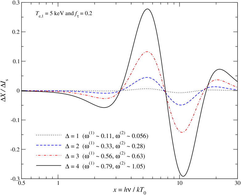
Refer to caption
Figure 6: Importance of higher order moments for a two-temperature plasma. We assumed Te,1=5keVsubscript𝑇e15keVT_{\rm e,1}=5\,{\rm keV} and fτ=0.2subscript𝑓𝜏0.2f_{\tau}=0.2. The absolute difference of the full two-temperature distortion, ΔItwoTΔsubscript𝐼two𝑇\Delta I_{{\rm two}-T}, and the approximation ΔIapprΔsubscript𝐼appr\Delta I_{\rm appr} which only uses the average SZ temperature and the temperature dispersion, ω(1)superscript𝜔1\omega^{(1)}, is shown in units of ΔIs0.013MJysr1similar-to-or-equalsΔsubscript𝐼s0.013MJysuperscriptsr1\Delta I_{\rm s}\simeq 0.013\,{\rm MJy\,sr^{-1}} (i.e., ΔX=ΔItwoTΔIapprΔ𝑋Δsubscript𝐼two𝑇Δsubscript𝐼appr\Delta X=\Delta I_{{\rm two}-T}-\Delta I_{\rm appr}). The temperature difference was varied in each case as annotated.

3.3 SZ signal for a two-temperature plasma

In the previous section we illustrated how the SZ signal is affected by the temperature profile of the cluster. However, for the analysis we used very smooth average profiles which allowed us to obtain an accurate description of the SZ signal with only a few new parameters (see Sect. 3.2). In general the variance of the temperature, density and velocity field along different lines-of-sight could be much larger than suggested by the simple average profiles.

One illustrative example is to consider a two-temperature plasma, with one low temperature, Te,1=Tesubscript𝑇e1subscript𝑇eT_{\rm e,1}=T_{\rm e}, and a high temperature region at Te,2=Te(1+Δ)subscript𝑇e2subscript𝑇e1ΔT_{\rm e,2}=T_{\rm e}(1+\Delta), where ΔΔ\Delta is the relative difference between the two temperatures. We furthermore have to specify the optical depths of each region, τ1=τ(1fτ)subscript𝜏1𝜏1subscript𝑓𝜏\tau_{1}=\tau(1-f_{\tau}) and τ2=fττsubscript𝜏2subscript𝑓𝜏𝜏\tau_{2}=f_{\tau}\tau, where τ𝜏\tau is the total optical depth along the line-of-sight. From this it follows

Te,SZsubscript𝑇eSZ\displaystyle T_{\rm e,SZ} =Te(1+fτΔ)absentsubscript𝑇e1subscript𝑓𝜏Δ\displaystyle=T_{\rm e}(1+f_{\tau}\Delta)
ω(1)superscript𝜔1\displaystyle\omega^{(1)} =fτ(1fτ)Δ2(1+fτΔ)2<fτ11absentsubscript𝑓𝜏1subscript𝑓𝜏superscriptΔ2superscript1subscript𝑓𝜏Δ2subscriptsuperscript𝑓1𝜏1\displaystyle=f_{\tau}\frac{(1-f_{\tau})\Delta^{2}}{(1+f_{\tau}\Delta)^{2}}<f^{-1}_{\tau}-1 (23)
ω(2)superscript𝜔2\displaystyle\omega^{(2)} =fτ(1fτ)(12fτ)Δ3(1+fτΔ)3<(fτ11)(fτ12)absentsubscript𝑓𝜏1subscript𝑓𝜏12subscript𝑓𝜏superscriptΔ3superscript1subscript𝑓𝜏Δ3subscriptsuperscript𝑓1𝜏1subscriptsuperscript𝑓1𝜏2\displaystyle=f_{\tau}\frac{(1-f_{\tau})(1-2f_{\tau})\Delta^{3}}{(1+f_{\tau}\Delta)^{3}}<(f^{-1}_{\tau}-1)(f^{-1}_{\tau}-2)

The temperature dispersion has a maximum at fτ=[2+Δ]1subscript𝑓𝜏superscriptdelimited-[]2Δ1f_{\tau}=[2+\Delta]^{-1} with ωmax(1)=14Δ2/[1+Δ]subscriptsuperscript𝜔1max14superscriptΔ2delimited-[]1Δ\omega^{(1)}_{\rm max}=\frac{1}{4}\Delta^{2}/[1+\Delta]. Furthermore, for Δ>[13fτ]1Δsuperscriptdelimited-[]13subscript𝑓𝜏1\Delta>[1-3f_{\tau}]^{-1} and fτ<1/3subscript𝑓𝜏13f_{\tau}<1/3 one finds ω(1)<ω(2)superscript𝜔1superscript𝜔2\omega^{(1)}<\omega^{(2)}.

Refer to caption
Figure 7: First few moments of the temperature field for a simulated cluster from Nagai et al. (2007b, a). We only show one projection; Te,SZsubscript𝑇eSZT_{\rm e,SZ} is in keV. We marked several regions for which we also computed the average SZ signal (see discussion in main text). The highest density peak (marked with an open circle) defines the cluster center. The box is 1Mpch11Mpcsuperscript11\,{\rm Mpc}\ h^{-1} on the side and the cluster mass is 3.8×10¹⁴Msimilar-to-or-equalsabsent3.8superscript1014subscript𝑀direct-product\simeq 3.8\times 10^{14}\,M_{\odot}.

In Fig. 6 we illustrate the importance of higher order temperature moments for a two-temperature plasma with Te,1subscript𝑇e1T_{\rm e,1} and fτ=0.2subscript𝑓𝜏0.2f_{\tau}=0.2 and different values of ΔΔ\Delta. For rather small temperature ratio the average SZ signal is approximated very well using the average SZ temperature and ω(1)superscript𝜔1\omega^{(1)}, with higher order temperature moments leading to very small corrections. For the most extreme case shown we have Te,1=5keVsubscript𝑇e15keVT_{\rm e,1}=5\,{\rm keV} and τ1=0.8subscript𝜏10.8\tau_{1}=0.8 with a high temperature component Te,1=25keVsubscript𝑇e125keVT_{\rm e,1}=25\,{\rm keV} and τ2=0.2subscript𝜏20.2\tau_{2}=0.2. In this case higher order moments are important at the level of a few percent for the SZ signal, but we found that the approximation improved dramatically when only adding ω(2)superscript𝜔2\omega^{(2)}. In this example one also had ω(1)<ω(2)superscript𝜔1superscript𝜔2\omega^{(1)}<\omega^{(2)}, a case that was not found for the smooth cluster profiles discussed in Sect. 3.2. Encountering ω(1)<ω(2)superscript𝜔1superscript𝜔2\omega^{(1)}<\omega^{(2)} therefore can be valued as indication of non-smooth, high variance plasma, possibly with more than one temperature component. However, to assess the statistical expectation for such cases detailed simulations of clusters within the cosmological context should be performed.

Table 2: Optical depth, SZ temperature, and first two line-of-sight temperature moments for the regions marked in Fig. 7.
Region τ[103]𝜏delimited-[]superscript103\tau\,[10^{-3}] Te,SZ[keV]subscript𝑇eSZdelimited-[]keVT_{\rm e,SZ}\,[\rm keV] ω(1)superscript𝜔1\omega^{(1)} ω(2)superscript𝜔2\omega^{(2)}
o 7.75637.75637.7563 4.10514.10514.1051 0.0664210.0664210.066421 0.0212540.0212540.021254
I 3.16823.16823.1682 6.31636.31636.3163 0.145380.145380.14538 0.0213780.021378-0.021378
II 0.622510.622510.62251 1.12511.12511.1251 0.692880.692880.69288 1.17971.17971.1797
III 1.37381.37381.3738 3.84623.84623.8462 0.295560.295560.29556 0.178440.178440.17844

3.4 Thermal SZ signal for a simulated cluster

We close our discussion of approximations of the SZ signal with one example taken from hydrodynamic simulations presented previously in Nagai et al. (2007b, a). The simulation is performed with the Adaptive Refinement Tree (ART) N𝑁N-body++gas-dynamics code (Kravtsov et al., 2002; Rudd et al., 2008), which is an Eulerian code that uses adaptive refinement in space and time, and non-adaptive refinement in mass to achieve the dynamic range necessary to resolve the cores of halos formed in self-consistent cosmological simulations. The simulation assumes a flat ΛΛ\LambdaCDM model: Ωm=1ΩΛ=0.3subscriptΩm1subscriptΩΛ0.3\Omega_{\rm m}=1-\Omega_{\Lambda}=0.3, Ωb=0.04286subscriptΩb0.04286\Omega_{\rm b}=0.04286, h=0.70.7h=0.7 and σ8=0.9subscript𝜎80.9\sigma_{8}=0.9, where the Hubble constant is defined as 100hkms1Mpc1100kmsuperscripts1superscriptMpc1100h{\ \rm km\ s^{-1}\ Mpc^{-1}}, and σ8subscript𝜎8\sigma_{8} is the mass variance within spheres of radius 8h18superscript18\,h^{-1} Mpc. The simulation shown here is of a cluster with mass M5003.8×1014Msimilar-to-or-equalssubscript𝑀5003.8superscript1014subscriptMdirect-productM_{500}\simeq 3.8\times 10^{14}\ {\rm M_{\odot}} undergoing a near 1:1 merger at z=0.25𝑧0.25z=0.25 (Nelson et al., 2012). The simulation was run using non-radiative gas dynamics on a uniform 1283superscript1283128^{3} grid with 8 levels of mesh refinement, corresponding to peak spatial resolution of 7h1similar-to-or-equalsabsent7superscript1\simeq 7\,h^{-1} kpc. The dark matter (DM) particle mass in the region around the cluster was mp9.1×108h1Msimilar-to-or-equalssubscript𝑚p9.1superscript108superscript1subscriptMdirect-productm_{\rm p}\simeq 9.1\times 10^{8}\,h^{-1}\,{\rm M_{\odot}}.

In Figure 7 we show projections of τ𝜏\tau, Te,SZsubscript𝑇eSZT_{\rm e,SZ}, ω(1)superscript𝜔1\omega^{(1)}, and ω(2)superscript𝜔2\omega^{(2)}. All variables are rather smooth close to the cluster center, but show significant variations in the outskirts. We marked regions with temperature variance ω(1)0.10.2similar-to-or-equalssuperscript𝜔10.10.2\omega^{(1)}\simeq 0.1-0.2 (see Table 2 for details). In these regions also ω(2)superscript𝜔2\omega^{(2)} acquired significant values, so that one could expect large contributions to the average SZ signal from higher order terms. The highest temperature region (marked with ‘I’) is slightly displaced from the maximum of the line-of-sight optical depth (marked by an open circle). It is also coinciding with a region of enhanced temperature variance. Region ‘II’ on the other hand is one of the coolest regions in the cluster but very large line-of-sight temperature variation.

We computed the SZ signal for the different regions using direct integration of the distortion for each frequency. We also confirmed that with the moment method developed in Sect. 2 gives the same result but at a significantly lower computational cost. In both cases, bulk velocity terms were omitted. We then compared the approximate SZ signal obtained with the moments summarized in Table 2 and found that the deviations were very small, consistent with higher order temperature moments being negligible. This indicates that even for more realistic cluster models the SZ signal is well approximated using the smooth profile expansion, Eq. (18). However, the considered cluster generally has rather low temperature so that relativistic corrections are not expected to be as important. We will investigate more massive clusters in our future work.

4 Effect of different line-of-sight variations on the SZ null

One of the important bands for SZ observations is defined by the SZ null. It is well-known that the position of the so called crossover frequency depends on the temperature of the cluster gas and average line-of-sight velocity. In particular, higher order temperature corrections affect its precise location (e.g., see Nozawa et al., 1998b). This is illustrated in Fig. 8, where the position of the null was computed using one of the functions implemented in SZpack. The results are in good agreement with the simple fitting formula given by Nozawa et al. (1998b).

However, it is clear that the line-of-sight temperature and velocity variations also affect the position of the null (see Fig. 9).
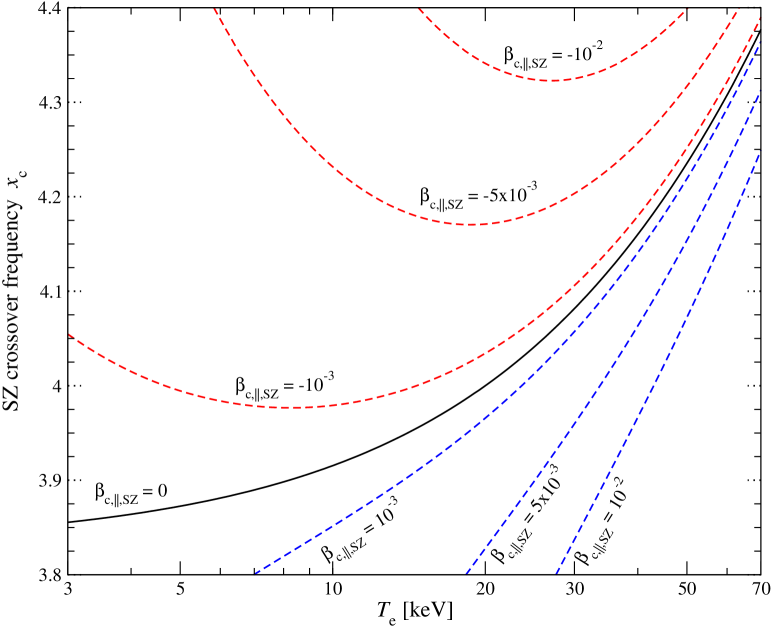
Refer to caption
Figure 8: Dependence of the crossover frequency on Te,SZsubscript𝑇eSZT_{\rm e,SZ} and βc,,SZ\beta_{\rm c,\parallel,SZ}.
Refer to caption
Refer to caption
Figure 9: Dependence of the crossover frequency on Te,SZsubscript𝑇eSZT_{\rm e,SZ}, ω(1)superscript𝜔1\omega^{(1)}, σ(1)superscript𝜎1\sigma^{(1)}, κ(1)superscript𝜅1\kappa^{(1)}, and βc,,SZ2subscriptsuperscript𝛽2cperpendicular-toSZ\beta^{2}_{\rm c,\perp,SZ}. We present the absolute shift, xcxc,0subscript𝑥csubscript𝑥c0x_{\rm c}-x_{\rm c,0}, where xc,0subscript𝑥c0x_{\rm c,0} is the case with βc,=ω(1)=σ(1)=κ(1)=βc,,SZ2=0\beta_{\rm c,\parallel}=\omega^{(1)}=\sigma^{(1)}=\kappa^{(1)}=\beta^{2}_{\rm c,\perp,SZ}=0.

Generally, the change in the position of the SZ null is rather small in the cases shown. The shift is nearly temperature-independent for σ(1)superscript𝜎1\sigma^{(1)}, while for ω(1)superscript𝜔1\omega^{(1)} it grows with Tesubscript𝑇eT_{\rm e}. We also present the effect of second order velocity terms on the crossover frequency. The line-of-sight variance of the velocity causes a decrease of the crossover frequency, while βc,,SZ2subscriptsuperscript𝛽2cperpendicular-toSZ\beta^{2}_{\rm c,\perp,SZ} leads to an increase. Both effects are rather small for a typical cluster temperature, even for the relatively large fiducial values that were chosen in the illustration. They furthermore practically cancel each other, indicating that for SZ parameter estimation they are degenerate. In the simulated cluster shown in Fig. 7 we found maximal values of βc,,SZ2105similar-to-or-equalssubscriptsuperscript𝛽2cperpendicular-toSZsuperscript105\beta^{2}_{\rm c,\perp,SZ}\simeq 10^{-5} and κ(1)105similar-to-or-equalssuperscript𝜅1superscript105\kappa^{(1)}\simeq 10^{-5}. However, this depends strongly on the chosen projection and post-merger time. It is therefore important to analyze a larger number of simulated clusters to estimate the typical values for βc,,SZ2subscriptsuperscript𝛽2cperpendicular-toSZ\beta^{2}_{\rm c,\perp,SZ} and κ(1)superscript𝜅1\kappa^{(1)}.

4.1 Effect on the deduced SZ temperature

The results of Fig. 9 indicate that conclusions on the temperature of the cluster drawn from measurements close to the SZ null can be affected by line-of-sight temperature and velocity variations. For instance, assuming βc,=0{\beta_{\rm c,\parallel}}=0, we find

xcsubscript𝑥c\displaystyle x_{\rm c} 3.83[1+0.011T^e8.6×105T^e2]absent3.83delimited-[]10.011subscript^𝑇e8.6superscript105superscriptsubscript^𝑇e2\displaystyle\approx 3.83[1+0.011\hat{T}_{\rm e}-8.6\times 10^{-5}\hat{T}_{\rm e}^{2}]
ΔxcΔsubscript𝑥c\displaystyle\Delta x_{\rm c} 0.042T^e[10.069T^e]ω(1)absent0.042subscript^𝑇edelimited-[]10.069subscript^𝑇esuperscript𝜔1\displaystyle\approx 0.042\hat{T}_{\rm e}[1-0.069\hat{T}_{\rm e}]\,\omega^{(1)} (24)

with T^e=Te/5keVsubscript^𝑇esubscript𝑇e5keV\hat{T}_{\rm e}=T_{\rm e}/5\,{\rm keV} for Te30keVless-than-or-similar-tosubscript𝑇e30keVT_{\rm e}\lesssim 30\,{\rm keV}. This means that for SZ temperature Te,SZ=5keVsubscript𝑇eSZ5keVT_{\rm e,SZ}=5\,{\rm keV} and ω(1)0.2similar-to-or-equalssuperscript𝜔10.2\omega^{(1)}\simeq 0.2, we find xc3.88subscript𝑥c3.88x_{\rm c}\approx 3.88, which would imply a temperature of Te,SZ6keVsimilar-to-or-equalssubscript𝑇eSZ6keVT_{\rm e,SZ}\simeq 6\,{\rm keV} when assuming ω(1)=0superscript𝜔10\omega^{(1)}=0 in the analysis. This is a 19%similar-to-or-equalsabsentpercent19\simeq 19\% bias towards higher temperature. More generally we find a bias of

ΔTeTe10.069T^e10.016T^eω(1)Δsubscript𝑇esubscript𝑇e10.069subscript^𝑇e10.016subscript^𝑇esuperscript𝜔1\displaystyle\frac{\Delta T_{\rm e}}{T_{\rm e}}\approx\frac{1-0.069\hat{T}_{\rm e}}{1-0.016\hat{T}_{\rm e}}\,\omega^{(1)} (25)

for Te30keVless-than-or-similar-tosubscript𝑇e30keVT_{\rm e}\lesssim 30\,{\rm keV}. The degeneracy between Tesubscript𝑇eT_{\rm e} and ω(1)superscript𝜔1\omega^{(1)} is very close to unity at low temperatures; however, for Te,SZ=30keVsubscript𝑇eSZ30keVT_{\rm e,SZ}=30\,{\rm keV} and ω(1)0.2similar-to-or-equalssuperscript𝜔10.2\omega^{(1)}\simeq 0.2 the temperature bias reduces to 13%similar-to-or-equalsabsentpercent13\simeq 13\%, which is also in good agreement with the behaviour found in Fig. 4. Although the absolute shift in xcsubscript𝑥cx_{\rm c} caused by ω(1)superscript𝜔1\omega^{(1)} increases with temperature (cf. Fig. 9), the relative shift decreases.

One can also estimate the effect of higher order velocity terms on the inferred value of Te,SZsubscript𝑇eSZT_{\rm e,SZ}. For contributions related to 𝒪(βc2)𝒪superscriptsubscript𝛽c2\mathcal{O}(\beta_{\rm c}^{2}) the effect is very small and only relevant for very low temperature gas, if at all. Similarly, the value of σ(1)superscript𝜎1\sigma^{(1)} is expected to be much smaller than 103less-than-or-similar-toabsentsuperscript103\lesssim 10^{-3}, unless high temperature gas also has large bulk velocity. For example, for the simulated cluster shown in Fig. 7 we found maximal values of σ(1)4.7×10⁴similar-to-or-equalssuperscript𝜎14.7superscript104\sigma^{(1)}\simeq 4.7\times 10^{-4}. Therefore the correction caused by ω(1)superscript𝜔1\omega^{(1)} is expected to be dominant, unless the overall temperature of the electron gas is very low.

As explained in Sect. 3.2.3, also variations caused by averaging the SZ signal over the beam introduce a dispersion. This has the same effect as the line-of-sight temperature variation, but for small beam the latter should again dominate.

4.2 Effect of frequency resolution on the SZ null

It is also straightforward to estimate the effect of the bandpass on the SZ null. The shift in its position is approximately given by

ΔxcΔsubscript𝑥c\displaystyle\Delta x_{\rm c} xc2S(xc)2xcS(xc)σx2absentsuperscriptsubscriptsubscript𝑥c2𝑆subscript𝑥c2subscriptsubscript𝑥c𝑆subscript𝑥csubscriptsuperscript𝜎2𝑥\displaystyle\approx-\frac{\partial_{x_{\rm c}}^{2}S(x_{\rm c})}{2\,\partial_{x_{\rm c}}S(x_{\rm c})}\,\sigma^{2}_{x}
0.2[10.32T^e+0.031T^e20.0018T^e3]σx2absent0.2delimited-[]10.32subscript^𝑇e0.031superscriptsubscript^𝑇e20.0018superscriptsubscript^𝑇e3subscriptsuperscript𝜎2𝑥\displaystyle\approx-0.2[1-0.32\hat{T}_{\rm e}+0.031\hat{T}_{\rm e}^{2}-0.0018\hat{T}_{\rm e}^{3}]\,\sigma^{2}_{x} (26)

for Te30keVless-than-or-similar-tosubscript𝑇e30keVT_{\rm e}\lesssim 30\,{\rm keV}. At Te23keVsimilar-to-or-equalssubscript𝑇e23keVT_{\rm e}\simeq 23\,{\rm keV} the shift in the crossover frequency caused by the average over the filter becomes small. Also, for a top-hat frequency filter one has σx2=Δx2/121.22(Δν/νc)2subscriptsuperscript𝜎2𝑥Δsuperscript𝑥212similar-to-or-equals1.22superscriptΔ𝜈subscript𝜈c2\sigma^{2}_{x}=\Delta x^{2}/12\simeq 1.22(\Delta\nu/\nu_{\rm c})^{2}, which for a bandwidth of 10%percent1010\% and Te5keVsimilar-to-or-equalssubscript𝑇e5keVT_{\rm e}\simeq 5\,{\rm keV} implies a shift of Δxc0.002similar-to-or-equalsΔsubscript𝑥c0.002\Delta x_{\rm c}\simeq-0.002 in the crossover frequency. This is expected to result in a 4%similar-to-or-equalsabsentpercent4\simeq 4\% bias of Tesubscript𝑇eT_{\rm e} towards lower values. More generally we find

ΔTeTe5.8T^e(Δννc)210.298T^e+0.024T^e20.0011T^e310.016T^eΔsubscript𝑇esubscript𝑇e5.8subscript^𝑇esuperscriptΔ𝜈subscript𝜈c210.298subscript^𝑇e0.024superscriptsubscript^𝑇e20.0011superscriptsubscript^𝑇e310.016subscript^𝑇e\displaystyle\frac{\Delta T_{\rm e}}{T_{\rm e}}\approx-\frac{5.8}{\hat{T}_{\rm e}}\left(\frac{\Delta\nu}{\nu_{\rm c}}\right)^{2}\frac{1-0.298\hat{T}_{\rm e}+0.024\hat{T}_{\rm e}^{2}-0.0011\hat{T}_{\rm e}^{3}}{1-0.016\hat{T}_{\rm e}} (27)

caused by the band-width of the frequency channel around xc(Te)subscript𝑥csubscript𝑇ex_{\rm c}(T_{\rm e}).

One should mention that we assumed that the frequency band is centered exactly on the crossover frequency, which of course changes with temperature, Tesubscript𝑇eT_{\rm e}. If the central frequency differs from xcsubscript𝑥cx_{\rm c} the response is also affected and hence the deduced temperature Tesubscript𝑇eT_{\rm e}. In the limit of very narrow bandpass this problem disappears, but otherwise this effect should be taken into account when interpreting SZ data at high precision.

5 SZ parameter estimation

In Sec. 2, we developed a new method for accurately calculating the mean SZ signal with relativistic corrections, and in Sec. 3 we extended this to include fluctuations in temperature and velocity along the line-of-sight for smooth cluster profiles. Subsets of the model parameters {τ,Te,SZ,ω(1,2,3),σ(1,2,3),κ(1,2,3),βc,,SZ,βc,,SZ2}\{\tau,T_{\rm e,SZ},\omega^{(1,2,3)},\sigma^{(1,2,3)},\kappa^{(1,2,3)},\beta_{\rm c,\parallel,SZ},\beta_{\rm c,\perp,SZ}^{2}\}, can then be estimated from measurements of the SZ spectrum999We will drop the subscript ‘SZ’ for convenience, but it is important to bear in mind that for instance the derived electron temperature, TeTe,SZsubscript𝑇esubscript𝑇eSZT_{\rm e}\equiv T_{\rm e,SZ}, i.e. it is weighted by the electron number density.. Here we describe an estimation of these parameters and their interpretation using a compilation of data and simulations. The parameters are estimated in a Markov Chain Monte Carlo (Foreman-Mackey et al., 2012) which is available with SZpack and can be adapted for particular experimental settings.

Rather than performing an exhaustive survey of experimental configurations and considerations, we describe a few informative cases. Even for a given combination of multi-band data, a complete interpretation is beyond the scope of this paper because it demands a consideration of contaminants, calibration errors, and offsets which can all be correlated across the bands. Particulars of the observation strategy may also need to be fully modelled (e.g., see Zemcov et al., 2012). The examples here are therefore meant to show some degeneracies and interpretative issues that arise in multi-band SZ parameter estimation. The same conclusions broadly apply to stacked cluster studies, except there, for example, the kSZ may average to zero.
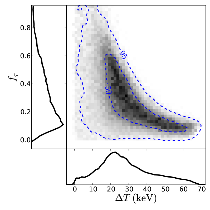
Refer to caption
Figure 10: Joint marginalized posterior distribution for a two-temperature model of the Bullet cluster showing the fractional optical depth fτsubscript𝑓𝜏f_{\tau} which can occupy a component of gas with temperature ΔTΔ𝑇\Delta T higher than the main component. Here, the temperature of the main component is (7.2±3.9)keVplus-or-minus7.23.9keV(7.2\pm 3.9)\,{\rm keV}. When the additional hot component is 202020 keV hotter, it can occupy a significant fraction of the optical depth while for larger excursions in temperature is must have progressively smaller optical depth. Note that non-zero ΔTΔ𝑇\Delta T is driven by the measurement at 857857857 GHz, where point source contamination could be significant.

5.1 Interpreting temperature variance in a recent SZ data compilation for the Bullet cluster

The simplest estimation problem which demonstrates evidence of temperature dispersion is the two-temperature model of Sec. 3.3. Here the parameters are a reference temperature Tesubscript𝑇eT_{\rm e}, a temperature difference ΔTΔ𝑇\Delta T, and the fractional optical depth fτ<1subscript𝑓𝜏1f_{\tau}<1 in the region with temperature Te+ΔTsubscript𝑇eΔ𝑇T_{\rm e}+\Delta T. A two-temperature case was also recently considered by Colafrancesco et al. (2011) as model for the Bullet cluster gas. The two SZ contributions from the gas at Tesubscript𝑇eT_{\rm e} and Te+ΔTsubscript𝑇eΔ𝑇T_{\rm e}+\Delta T are computed to all relevant relativistic correction orders using SZpack. Following the compilation of Prokhorov & Colafrancesco (2012), we consider data across the bands {150,275,600,857}GHz150275600857GHz\{150,275,600,857\}\,{\rm GHz} with mean values and errors of ΔI={0.325±0.015,0.21±0.077,0.268±0.031,0.097±0.019}MJy/srΔ𝐼plus-or-minus0.3250.015plus-or-minus0.210.077plus-or-minus0.2680.031plus-or-minus0.0970.019MJysr{\Delta I=}\{-0.325\pm 0.015,0.21\pm 0.077,0.268\pm 0.031,0.097\pm 0.019\}\,\rm MJy/sr from observations of Gomez et al. (2004) and Zemcov et al. (2010). We assume that τ=0.0138±0.0016𝜏plus-or-minus0.01380.0016\tau=0.0138\pm 0.0016 is known (Prokhorov & Colafrancesco, 2012) as a Gaussian prior probability distribution from X-ray observations. This helps break the strong degeneracy between τ𝜏\tau and Tesubscript𝑇eT_{\rm e}. For the latter we find Te=(7.2±3.9)keVsubscript𝑇eplus-or-minus7.23.9keVT_{\rm e}=(7.2\pm 3.9)\,{\rm keV}. Figure 10 shows the marginalized posterior distribution for ΔT=2511+19Δ𝑇subscriptsuperscript251911\Delta T=25^{+19}_{-11} keV and fτ=0.270.17+0.26subscript𝑓𝜏subscriptsuperscript0.270.260.17f_{\tau}=0.27^{+0.26}_{-0.17} (where two-sided errors are given for non-Gaussian distributions at percentiles {16%,50%,84%}percent16percent50percent84\{16\%,50\%,84\%\}, equivalent to 1σ1𝜎1\sigma in a normal distribution). Conclusions from a model with βc,\beta_{\rm c,\parallel} (taken to be the same for both components) as a free parameter are similar at this level of uncertainty.

We next consider an ICM model with line-of-sight temperature dispersion about the mean using the free parameters {τ,Te,ω(1)}𝜏subscript𝑇esuperscript𝜔1\{\tau,T_{\rm e},\omega^{(1)}\}, where ω(1)=Te2/[τTe,SZ2]1superscript𝜔1delimited-⟨⟩superscriptsubscript𝑇e2delimited-[]𝜏superscriptsubscript𝑇eSZ21\omega^{(1)}=\langle T_{\rm e}^{2}\rangle/[\tau T_{\rm e,SZ}^{2}]-1 is a measure of the temperature dispersion (see Sect. 3.2). In this case, we obtain Te=(13.5±1.8)keVsubscript𝑇eplus-or-minus13.51.8keVT_{\rm e}=(13.5\pm 1.8)\,{\rm keV} and ω(1)=0.8±0.4superscript𝜔1plus-or-minus0.80.4\omega^{(1)}=0.8\pm 0.4 with a modest correlation corr(Te,ω(1))=0.4corrsubscript𝑇esuperscript𝜔10.4{\rm corr}(T_{\rm e},\omega^{(1)})=-0.4. When βc,\beta_{\rm c,\parallel} is added as a free parameter, we find Te=(13.1±2.0)keVsubscript𝑇eplus-or-minus13.12.0keVT_{\rm e}=(13.1\pm 2.0)\,{\rm keV} and ω(1)=1.0±0.6superscript𝜔1plus-or-minus1.00.6\omega^{(1)}=1.0\pm 0.6 with βc,=(1.7±2.1)×103\beta_{\rm c,\parallel}=(-1.7\pm 2.1)\times 10^{-3} and corr(βc,,ω(1))=0.6{\rm corr}(\beta_{\rm c,\parallel},\omega^{(1)})=-0.6, showing that there is no significant indication of non-zero line-of-sight bulk velocity. We can extend the fit to include ω(2)superscript𝜔2\omega^{(2)}, a measure of the skewness in the temperature distribution. Here, ω(1)=1.1±0.6superscript𝜔1plus-or-minus1.10.6\omega^{(1)}=1.1\pm 0.6 and ω(2)=2.0±2.6superscript𝜔2plus-or-minus2.02.6\omega^{(2)}=2.0\pm 2.6 (no strong evidence for more than dispersion) with a strong correlation, corr(ω(1),ω(2))=0.75corrsuperscript𝜔1superscript𝜔20.75{\rm corr}(\omega^{(1)},\omega^{(2)})=0.75. It is also informative to compare with a model where ω(1)superscript𝜔1\omega^{(1)} is fixed to zero and only Tesubscript𝑇eT_{\rm e} and τ𝜏\tau vary. In this case, Te=(14.8±2.1)keVsubscript𝑇eplus-or-minus14.82.1keVT_{\rm e}=(14.8\pm 2.1)\,{\rm keV}, but as shown in Fig. 11, this is a poorer fit to the data because it lacks the freedom to explain the flux measurement at 857857857 GHz.

The two previous models depart from the first reported measurement of temperature dispersion by Prokhorov & Colafrancesco (2012), where the temperature expansion is used directly to constrain the variance:

ΔIIoΔ𝐼subscript𝐼o\displaystyle\frac{\Delta I}{{I_{\rm o}}} τ[g0(x)kTemec2+g1(x)(kTe)2me2c4+g2(x)(kTe)3me3c6].absent𝜏delimited-[]subscript𝑔0𝑥delimited-⟨⟩𝑘subscript𝑇esubscript𝑚esuperscript𝑐2subscript𝑔1𝑥delimited-⟨⟩superscript𝑘subscript𝑇e2superscriptsubscript𝑚e2superscript𝑐4subscript𝑔2𝑥delimited-⟨⟩superscript𝑘subscript𝑇e3superscriptsubscript𝑚e3superscript𝑐6\displaystyle\approx\tau\biggl{[}g_{0}(x)\,\frac{\langle kT_{\rm e}\rangle}{m_{\rm e}c^{2}}+g_{1}(x)\,\frac{\langle(kT_{\rm e})^{2}\rangle}{m_{\rm e}^{2}c^{4}}+g_{2}(x)\,\frac{\langle(kT_{\rm e})^{3}\rangle}{m_{\rm e}^{3}c^{6}}\biggr{]}. (28)

Here g0subscript𝑔0g_{0}, g1subscript𝑔1g_{1} and g2subscript𝑔2g_{2} are the spectral functions of the asymptotic expansion given in Challinor & Lasenby (1998) and flux normalization, Io(2h/c2)(kT0/h)3270MJysr1subscript𝐼o2superscript𝑐2superscript𝑘subscript𝑇03270MJysuperscriptsr1{I_{\rm o}}\equiv(2h/c^{2})(kT_{0}/h)^{3}\approx 270\,{\rm MJy\,sr^{-1}}. The temperature variance can be inferred directly through σ2=(kTe)2kTe2superscript𝜎2delimited-⟨⟩superscript𝑘subscript𝑇e2superscriptdelimited-⟨⟩𝑘subscript𝑇e2\sigma^{2}=\langle(kT_{\rm e})^{2}\rangle-\langle kT_{\rm e}\rangle^{2}, by fitting for the coefficients of g0subscript𝑔0g_{0}, g1subscript𝑔1g_{1} and g2subscript𝑔2g_{2}. As a check of the MCMC here, we find a temperature variance of (9.2±2.5)plus-or-minus9.22.5(9.2\pm 2.5) keV, in agreement with (9.5±2.6)plus-or-minus9.52.6(9.5\pm 2.6) keV reported in Prokhorov & Colafrancesco (2012). The average temperature of the Bullet cluster inferred from X-ray observations (Million & Allen, 2009) is 14.514.514.5 keV. At these temperatures, Fig. 2 shows that the asymptotic expansion is a poor approximation even to order (kTe)10/(mec2)10delimited-⟨⟩superscript𝑘subscript𝑇e10superscriptsubscript𝑚esuperscript𝑐210\langle(kT_{\rm e})^{10}\rangle/(m_{\rm e}c^{2})^{10}, which worsens for higher temperature excursions. Because the first few moments do not adequately describe the mean relativistic corrections, it is also difficult to interpret the dispersion inferred from the first two moments in Eq. (28). Nevertheless, converting the moment constraints, we find that Te=(13.7±1.9)subscript𝑇eplus-or-minus13.71.9T_{\rm e}=(13.7\pm 1.9) keV and ω(1)σ2/Te2=(0.5±0.3)similar-tosuperscript𝜔1superscript𝜎2superscriptsubscript𝑇e2plus-or-minus0.50.3\omega^{(1)}\sim\sigma^{2}/T_{\rm e}^{2}=(0.5\pm 0.3) for this model, which is consistent with the dispersion measured above. However, as the experimental sensitivity and frequency coverage increases the model given by Eq. (28) should lead to biased values for Tesubscript𝑇eT_{\rm e} and ω(1)superscript𝜔1\omega^{(1)}.

Refer to caption
Figure 11: Mean SZ spectra for four models of the data (black points) (Prokhorov & Colafrancesco, 2012). A model including only Tesubscript𝑇eT_{\rm e} with relativistic corrections at all relevant orders (yellow) does not have the freedom to describe the 857857857 GHz flux, and drives the temperature up. An asymptotic expansion of relativistic corrections to order (kTe)3/(mec2)3delimited-⟨⟩superscript𝑘subscript𝑇e3superscriptsubscript𝑚esuperscript𝑐23\langle(kT_{\rm e})^{3}\rangle/(m_{\rm e}c^{2})^{3} (red) describes the data, but is insufficiently converged to self-consistently explain the relativistic corrections to the SZ flux. The green curve is a model with two regions of different temperature and the blue curve is a model with dispersion about a mean temperature (both cases include all relevant orders in the relativistic corrections). Measurements around and above the SZ maximum have the potential to differentiate these models, while close to the SZ null and below all models practically coincide.

In any of the models above, the detection of dispersion is driven by the flux measurement at 857857857 GHz. Removing that measurement from the two-temperature model parameter estimation results in an upper bound rather than detection (ΔT<56Δ𝑇56\Delta T<56 keV, 95%percent9595\% confidence). In the dispersion model with parameters {Te,τ,ω(1)}subscript𝑇e𝜏superscript𝜔1\{T_{\rm e},\tau,\omega^{(1)}\}, we find ω(1)=0.4±0.7superscript𝜔1plus-or-minus0.40.7\omega^{(1)}=0.4\pm 0.7. Most of the constraint on relativistic effects and dispersion comes from above the SZ null, but in this frequency region it becomes more difficult to separate point source contamination, both because IR fluxes increase at higher frequency and because both the SZ and contamination are positive fluxes.

The parameter estimates here are based on flux measurements in four frequencies, and yield qualitatively similar conclusions for the current sensitivity. Across a range of frequencies, however, the three models do predict different SZ spectra, shown in Fig. 11. Here, the expression of Eq. (28) shows the most variation with respect to other models with temperature dispersion because three temperature moments in the asymptotic series do not fully describe the relativistic corrections and temperature dispersion. The other two models show slight differences above the SZ maximum, indicating that more precise measurements at a wider range of frequencies could help differentiate between physical interpretations of the dispersion. Still the differences in the SZ signal above the null are not much larger than 5%10%similar-to-or-equalsabsentpercent5percent10\simeq 5\%-10\%. There are limited transparency windows in the atmosphere, but at frequencies above the null, instruments can achieve similar resolution and sensitivity with comparatively smaller apertures, so that balloon and space-borne instruments could have the potential to constrain these frequency regions. Note that the distortion around the null is virtually identical in all the models described here.

In the constraints above, we neglected the finite bandwidth of the observations. It is customary to define an effective band center for a given spectral index as the frequency at which the measured flux matches the true flux. We can expand smooth spectra about this effective band center and see that the linear term drops out and that the change in center is due to the second derivative curvature of the spectrum across the band (see Sect 4.2). The extent of this effect depends on experiment-dependent parameters, but as a rough estimate, a 10%percent1010\% bandwidth near the maximum at x7similar-to𝑥7x\sim 7 can produce a nearly 10%percent1010\% bias. In the data considered above, for a 10%percent1010\% bandwidth, we find Te=(13.6±1.8)subscript𝑇eplus-or-minus13.61.8T_{\rm e}=(13.6\pm 1.8) keV and ω(1)=0.72±0.4superscript𝜔1plus-or-minus0.720.4\omega^{(1)}=0.72\pm 0.4, a shift which can be neglected here, but should become important as the measurements improve.

We can also examine the impact of improved measurements on the inference of ω(1)superscript𝜔1\omega^{(1)}. Fig. 12 considers the parameter set {τ,Te,ω(1)}𝜏subscript𝑇esuperscript𝜔1\{\tau,T_{\rm e},\omega^{(1)}\} under improvements to the dataset used in Prokhorov & Colafrancesco (2012). By reducing the SZ measurement errors a factor of five for the same τ𝜏\tau prior, the ω(1)Tesuperscript𝜔1subscript𝑇e\omega^{(1)}-T_{\rm e} correlation increases to 0.70.7-0.7 and the parameter errors improve modestly. Both the correlation and residual uncertainty are driven by the imperfect τ𝜏\tau prior, and deeper SZ measurements have little additional benefit. Shrinking the τ𝜏\tau prior by a factor of five on top of the improved SZ flux measurements significantly improves these constraints. This also emphasizes the importance of combining SZ measurement with X-ray observations to break degeneracies among model parameters.
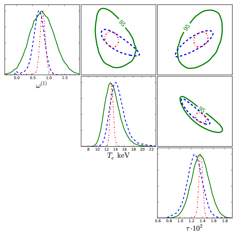
Refer to caption
Figure 12: Posterior distributions of {Te,τ,ω(1)}subscript𝑇e𝜏superscript𝜔1\{T_{\rm e},\tau,\omega^{(1)}\} achieved by improvements to the measurements compiled in Prokhorov & Colafrancesco (2012). The green solid line gives 1D marginalized probabilities and 2D contours (95%percent9595\% enclosed) for the original dataset. This shows a clear indication of scatter about the central temperature through significantly non-zero ω(1)superscript𝜔1\omega^{(1)}. Improving the SZ flux measurements by a factor of five (keeping the measured central values) only improves the constraint on Tesubscript𝑇eT_{\rm e} and ω(1)superscript𝜔1\omega^{(1)} (blue dashed line) modestly because of their degeneracy with τ𝜏\tau. Additionally shrinking the τ𝜏\tau prior errors by a factor of five (red dot-dashed line) breaks this to yield the strongest constraints.

6 Discussion and conclusion

We developed a novel method for extracting information about the state of the ICM from SZ observations which is based on moments of the cluster’s temperature and velocity field. Both a quasi-exact approach (Sect. 2), which should be useful for computing the precise SZ signal from simulated clusters in an efficient manner, and an approximate treatment based on the smoothness of the cluster profile (Sect. 3.2) were considered. In future SZ parameter estimation and cluster profile reconstruction the latter method should be widely applicable, with the main SZ observables consisting of a small number of parameters, 𝒑={τ,Te,SZ,ω(1,2,3),σ(1,2,3),κ(1,2,3),βc,,SZ,βc,,SZ2}\mbox{\boldmath${p}$\unboldmath}=\{\tau,T_{\rm e,SZ},\omega^{(1,2,3)},\sigma^{(1,2,3)},\kappa^{(1,2,3)},\beta_{\rm c,\parallel,SZ},\beta_{\rm c,\perp,SZ}^{2}\}. Maps of these parameters allow very precise representation of the SZ signal and hence a compression of the observational data to only spatially dependent variables. These can be directly used in the inversion problem that determines the cluster temperature and velocity structure.

Our discussion of different cluster models indicated that the above compression of the data should work even in more general cases, when the line-of-sight temperature and velocity distributions become non-trivial. The reason is simply that the SZ signal itself is very smooth in frequency and higher order temperature and velocity moments contribute in a diminishing manner, once the average SZ signal (which includes a large number of temperature correction terms) is taken out. We also showed how the position of the SZ null is affected by temperature variations along the line-of-sight. If neglected this can lead to biases in the deduced electron temperature at the level of 10%20%similar-to-or-equalsabsentpercent10percent20\simeq 10\%-20\% (see Eq. 25). Velocity correction terms, beyond the normal kSZ effect, are generally expected to be less important; however, a more detailed study using hydrodynamic cluster simulations is needed to give a more quantitative answer about the typical magnitude of different terms.

We furthermore illustrated the importance of high frequency channels for distinguishing different cluster atmospheres (Fig. 11) using recent data for the Bullet cluster (Prokhorov & Colafrancesco, 2012). Our analysis indicates that presently at two-temperature model remains indistinguishable from a cluster model with line-of-sight temperature variance, but a single temperature model is in tension with the measured SZ flux at 857GHz857GHz857\,{\rm GHz}. We also explain why the results for the temperature dispersion deduced with an asymptotic expansion of the SZ signal are difficult to interpret. In the future, it will be important to consider foregrounds and systematic effects in more detail. Also additional physical effect, e.g., multiple-scattering effects (Dolgov et al., 2001) or the SZ effect for non-thermal electron populations (Enßlin & Kaiser, 2000), should be taken into account. We plan to extend SZpack with these features in another publication.

To realize the full power of SZ measurement as a cosmological probe, studies of individual clusters and their atmosphere will become very important. It is especially critical to extend the studies of thermodynamic and velocity structures to the outskirts of high-redshift clusters in order to understand the biases in the global properties of galaxy clusters and their evolution across the cosmic time. Because the SZ signal is independent of redshift and linearly proportional to the gas density, high-resolution SZ observations can enable detailed studies of the ICM structure in the outskirts of high-redshift clusters, and hence are highly complimentary to X-ray observations whose sensitivities are limited to the inner regions of clusters or the outskirts of nearby systems. The combination of future spectroscopic X-ray measurements with high resolution SZ data will open new opportunities for studying cluster astrophysics, and the moment method developed here provides one important step in this direction.

Acknowledgments

We thanks Eiichiro Komatsu, Andrea Morandi, and Michael Zemcov for valuable comments and discussion. DN and KN acknowledge the support from the NSF grant AST-1009811, the NASA ATP grant NNX11AE07G, the NASA Chandra Theory grant GO213004B, Research Corporation, and by Yale University. This work was supported in part by the facilities and staff of the Yale University Faculty of Arts and Sciences High Performance Computing Center.

Appendix A Definition of functions for asymptotic expansion

From Eq. (25) of CNSN we can directly identify

Mklowsubscriptsuperscript𝑀low𝑘\displaystyle M^{\rm low}_{k} =Ykkin+16𝒟xYk13𝒟xDkkinabsentsubscriptsuperscript𝑌kin𝑘16subscript𝒟𝑥subscript𝑌𝑘13subscriptsuperscript𝒟𝑥subscriptsuperscript𝐷kin𝑘\displaystyle=Y^{\rm kin}_{k}+\frac{1}{6}\mathcal{D}_{x}Y_{k}-\frac{1}{3}\mathcal{D}^{\ast}_{x}D^{\rm kin}_{k}
Dklowsubscriptsuperscript𝐷low𝑘\displaystyle D^{\rm low}_{k} =DkkinxxYkabsentsubscriptsuperscript𝐷kin𝑘𝑥subscript𝑥subscript𝑌𝑘\displaystyle=D^{\rm kin}_{k}-x\,\partial_{x}Y_{k} (29)
Qklowsubscriptsuperscript𝑄low𝑘\displaystyle Q^{\rm low}_{k} =Qkkin+13x2x2Yk+23𝒟xDkkin.absentsubscriptsuperscript𝑄kin𝑘13superscript𝑥2subscriptsuperscript2𝑥subscript𝑌𝑘23subscriptsuperscript𝒟absent𝑥subscriptsuperscript𝐷kin𝑘\displaystyle=Q^{\rm kin}_{k}+\frac{1}{3}x^{2}\partial^{2}_{x}Y_{k}+\frac{2}{3}\mathcal{D}^{\ast\ast}_{x}D^{\rm kin}_{k}.

The functions Yksubscript𝑌𝑘Y_{k}, Ykkinsubscriptsuperscript𝑌kin𝑘Y^{\rm kin}_{k}, Dkkinsubscriptsuperscript𝐷kin𝑘D^{\rm kin}_{k}, and Qkkinsubscriptsuperscript𝑄kin𝑘Q^{\rm kin}_{k} are all defined in CNSN. The differential operators are 𝒟x=3xx+x2x2subscript𝒟𝑥3𝑥subscript𝑥superscript𝑥2subscriptsuperscript2𝑥\mathcal{D}_{x}=3x\,\partial_{x}+x^{2}\partial^{2}_{x}, 𝒟x=2+xxsubscriptsuperscript𝒟𝑥2𝑥subscript𝑥\mathcal{D}^{\ast}_{x}=2+x\,\partial_{x}, and 𝒟x=1xxsubscriptsuperscript𝒟absent𝑥1𝑥subscript𝑥\mathcal{D}^{\ast\ast}_{x}=1-x\,\partial_{x}. With the relations given in CNSN it is straightforward to show that

xxYn𝑥subscript𝑥subscript𝑌𝑛\displaystyle x\,\partial_{x}Y_{n} =k=12n+2ak(n)[kΔxk+Δxk+1]nPl(x)absentsuperscriptsubscript𝑘12𝑛2superscriptsubscript𝑎𝑘𝑛delimited-[]𝑘subscriptsuperscriptΔ𝑘𝑥subscriptsuperscriptΔ𝑘1𝑥subscript𝑛Pl𝑥\displaystyle=\sum_{k=1}^{2n+2}a_{k}^{(n)}\left[k\,\Delta^{k}_{x}+\Delta^{k+1}_{x}\right]n_{\rm Pl}(x)
x2x2Ynsuperscript𝑥2subscriptsuperscript2𝑥subscript𝑌𝑛\displaystyle x^{2}\partial^{2}_{x}Y_{n} =k=12n+2ak(n)[k(k1)Δxk+2kΔxk+1+Δxk+2]nPl(x)absentsuperscriptsubscript𝑘12𝑛2superscriptsubscript𝑎𝑘𝑛delimited-[]𝑘𝑘1subscriptsuperscriptΔ𝑘𝑥2𝑘subscriptsuperscriptΔ𝑘1𝑥subscriptsuperscriptΔ𝑘2𝑥subscript𝑛Pl𝑥\displaystyle=\sum_{k=1}^{2n+2}a_{k}^{(n)}\left[k(k-1)\,\Delta^{k}_{x}+2k\,\Delta^{k+1}_{x}+\Delta^{k+2}_{x}\right]n_{\rm Pl}(x)
𝒟xYnsubscript𝒟𝑥subscript𝑌𝑛\displaystyle\mathcal{D}_{x}Y_{n} =6Ynkinabsent6subscriptsuperscript𝑌kin𝑛\displaystyle=6\,Y^{\rm kin}_{n} (30)
𝒟xDnkinsubscriptsuperscript𝒟𝑥subscriptsuperscript𝐷kin𝑛\displaystyle\mathcal{D}^{\ast}_{x}D^{\rm kin}_{n} =k=02n+2dk(n)[k(k+2)Δxk+(2k+3)Δxk+1+Δxk+2]nPl(x)absentsuperscriptsubscript𝑘02𝑛2superscriptsubscript𝑑𝑘𝑛delimited-[]𝑘𝑘2superscriptsubscriptΔ𝑥𝑘2𝑘3superscriptsubscriptΔ𝑥𝑘1superscriptsubscriptΔ𝑥𝑘2subscript𝑛Pl𝑥\displaystyle=\sum_{k=0}^{2n+2}d_{k}^{(n)}\left[k(k+2)\,\Delta_{x}^{k}+(2k+3)\,\Delta_{x}^{k+1}+\Delta_{x}^{k+2}\right]n_{\rm Pl}(x)
𝒟xDnkinsubscriptsuperscript𝒟absent𝑥subscriptsuperscript𝐷kin𝑛\displaystyle\mathcal{D}^{\ast\ast}_{x}D^{\rm kin}_{n} =k=02n+2dk(n)[k(k1)Δxk+2kΔxk+1+Δxk+2]nPl(x)absentsuperscriptsubscript𝑘02𝑛2superscriptsubscript𝑑𝑘𝑛delimited-[]𝑘𝑘1subscriptsuperscriptΔ𝑘𝑥2𝑘subscriptsuperscriptΔ𝑘1𝑥subscriptsuperscriptΔ𝑘2𝑥subscript𝑛Pl𝑥\displaystyle=-\sum_{k=0}^{2n+2}d_{k}^{(n)}\left[k(k-1)\,\Delta^{k}_{x}+2k\,\Delta^{k+1}_{x}+\Delta^{k+2}_{x}\right]n_{\rm Pl}(x)

with nPl(x)=1/[ex1]subscript𝑛Pl𝑥1delimited-[]superscript𝑒𝑥1n_{\rm Pl}(x)=1/[e^{x}-1] and Δxk=xkxksuperscriptsubscriptΔ𝑥𝑘superscript𝑥𝑘subscriptsuperscript𝑘𝑥\Delta_{x}^{k}=x^{k}\partial^{k}_{x}. This implies

Mnlowsubscriptsuperscript𝑀low𝑛\displaystyle M^{\rm low}_{n} =13k=02n+2(ak(n)dk(n))[k(k+2)Δxk+(2k+3)Δxk+1+Δxk+2]nPlabsent13superscriptsubscript𝑘02𝑛2superscriptsubscript𝑎𝑘𝑛superscriptsubscript𝑑𝑘𝑛delimited-[]𝑘𝑘2subscriptsuperscriptΔ𝑘𝑥2𝑘3subscriptsuperscriptΔ𝑘1𝑥subscriptsuperscriptΔ𝑘2𝑥subscript𝑛Pl\displaystyle=\frac{1}{3}\sum_{k=0}^{2n+2}(a_{k}^{(n)}-d_{k}^{(n)})\left[k(k+2)\,\Delta^{k}_{x}+(2k+3)\,\Delta^{k+1}_{x}+\Delta^{k+2}_{x}\right]n_{\rm Pl}
Dnlowsubscriptsuperscript𝐷low𝑛\displaystyle D^{\rm low}_{n} =k=02n+2(dk(n)ak(n))[kΔxk+Δxk+1]nPl(x)absentsuperscriptsubscript𝑘02𝑛2superscriptsubscript𝑑𝑘𝑛superscriptsubscript𝑎𝑘𝑛delimited-[]𝑘subscriptsuperscriptΔ𝑘𝑥subscriptsuperscriptΔ𝑘1𝑥subscript𝑛Pl𝑥\displaystyle=\sum_{k=0}^{2n+2}(d_{k}^{(n)}-a_{k}^{(n)})\left[k\,\Delta^{k}_{x}+\Delta^{k+1}_{x}\right]n_{\rm Pl}(x) (31)
Qnlowsubscriptsuperscript𝑄low𝑛\displaystyle Q^{\rm low}_{n} =13k=02n+2(ak(n)+qk(n)2dk(n))[k(k1)Δxk+2kΔxk+1+Δxk+2]nPlabsent13superscriptsubscript𝑘02𝑛2superscriptsubscript𝑎𝑘𝑛superscriptsubscript𝑞𝑘𝑛2superscriptsubscript𝑑𝑘𝑛delimited-[]𝑘𝑘1subscriptsuperscriptΔ𝑘𝑥2𝑘subscriptsuperscriptΔ𝑘1𝑥subscriptsuperscriptΔ𝑘2𝑥subscript𝑛Pl\displaystyle=\frac{1}{3}\sum_{k=0}^{2n+2}(a_{k}^{(n)}+q_{k}^{(n)}-2d_{k}^{(n)})\left[k(k-1)\,\Delta^{k}_{x}+2k\,\Delta^{k+1}_{x}+\Delta^{k+2}_{x}\right]n_{\rm Pl}

We extended the sums for Yksubscript𝑌𝑘Y_{k} and its derivatives to k=0𝑘0k=0 using a0(n)=0superscriptsubscript𝑎0𝑛0a_{0}^{(n)}=0 for n0𝑛0n\geq 0.

Appendix B Definition of functions for the improved basis set

It is straightforward to transform the set of basis functions given in CNSN from the cluster frame into the CMB rest frame. However, to obtain the expressions for Ykhighsubscriptsuperscript𝑌high𝑘Y^{\rm high}_{k}, Mkhighsubscriptsuperscript𝑀high𝑘M^{\rm high}_{k}, Dkhighsubscriptsuperscript𝐷high𝑘D^{\rm high}_{k}, and Qkhighsubscriptsuperscript𝑄high𝑘Q^{\rm high}_{k}, a few intermediate steps are needed. Using the definitions of CNSN gives

Ykhigh,subscriptsuperscript𝑌high𝑘\displaystyle Y^{\rm high,\ast}_{k} =Zkabsentsubscript𝑍𝑘\displaystyle=Z_{k}
Mkhigh,subscriptsuperscript𝑀high𝑘\displaystyle M^{\rm high,\ast}_{k} =Zkkin+16𝒟xZk13𝒟xCkkinabsentsubscriptsuperscript𝑍kin𝑘16subscript𝒟𝑥subscript𝑍𝑘13subscriptsuperscript𝒟𝑥subscriptsuperscript𝐶kin𝑘\displaystyle=Z^{\rm kin}_{k}+\frac{1}{6}\mathcal{D}_{x}Z_{k}-\frac{1}{3}\mathcal{D}^{\ast}_{x}C^{\rm kin}_{k}
Dkhigh,subscriptsuperscript𝐷high𝑘\displaystyle D^{\rm high,\ast}_{k} =CkkinxxZkabsentsubscriptsuperscript𝐶kin𝑘𝑥subscript𝑥subscript𝑍𝑘\displaystyle=C^{\rm kin}_{k}-x\,\partial_{x}Z_{k} (32)
Qkhigh,subscriptsuperscript𝑄high𝑘\displaystyle Q^{\rm high,\ast}_{k} =Skkin+13x2x2Zk+23𝒟xCkkin.absentsubscriptsuperscript𝑆kin𝑘13superscript𝑥2subscriptsuperscript2𝑥subscript𝑍𝑘23subscriptsuperscript𝒟absent𝑥subscriptsuperscript𝐶kin𝑘\displaystyle=S^{\rm kin}_{k}+\frac{1}{3}x^{2}\partial^{2}_{x}Z_{k}+\frac{2}{3}\mathcal{D}^{\ast\ast}_{x}C^{\rm kin}_{k}.

These can be used like the functions Ykhighsubscriptsuperscript𝑌high𝑘Y^{\rm high}_{k}, Mkhighsubscriptsuperscript𝑀high𝑘M^{\rm high}_{k}, Dkhighsubscriptsuperscript𝐷high𝑘D^{\rm high}_{k}, and Qkhighsubscriptsuperscript𝑄high𝑘Q^{\rm high}_{k} in Eq. (7) but with 𝒩(θe)θek𝒩(θe)(θeθe,0)k/𝒩(θe,0)𝒩subscript𝜃esuperscriptsubscript𝜃e𝑘𝒩subscript𝜃esuperscriptsubscript𝜃esubscript𝜃e0𝑘𝒩subscript𝜃e0\mathcal{N}(\theta_{\rm e})\,\theta_{\rm e}^{k}\rightarrow\mathcal{N}(\theta_{\rm e})\,(\theta_{\rm e}-\theta_{\rm e,0})^{k}/\mathcal{N}(\theta_{\rm e,0}). Since

𝒩(θe)𝒩(θe,0)(θeθe,0)k1𝒩(θe,0)m=0k(km)(θe,0)km𝒩(θe)θem𝒩subscript𝜃e𝒩subscript𝜃e0superscriptsubscript𝜃esubscript𝜃e0𝑘1𝒩subscript𝜃e0superscriptsubscript𝑚0𝑘binomial𝑘𝑚superscriptsubscript𝜃e0𝑘𝑚𝒩subscript𝜃esuperscriptsubscript𝜃e𝑚\displaystyle\frac{\mathcal{N}(\theta_{\rm e})}{\mathcal{N}(\theta_{\rm e,0})}\left(\theta_{\rm e}-\theta_{\rm e,0}\right)^{k}\!\equiv\frac{1}{\mathcal{N}(\theta_{\rm e,0})}\,\sum_{m=0}^{k}\binom{k}{m}\,(-\theta_{\rm e,0})^{k-m}\,\mathcal{N}(\theta_{\rm e})\,\theta_{\rm e}^{m} (33)

by defining the lower triangular matrix, Tij=1𝒩(θe,0)(ij)(θe,0)ijsubscript𝑇𝑖𝑗1𝒩subscript𝜃e0binomial𝑖𝑗superscriptsubscript𝜃e0𝑖𝑗T_{ij}=\frac{1}{\mathcal{N}(\theta_{\rm e,0})}\,\binom{i}{j}\,(-\theta_{\rm e,0})^{i-j}, we have the transformation 𝑿high=𝗧T𝑿high,superscript𝑿highsuperscript𝗧𝑇superscript𝑿high\mbox{\boldmath${X}$\unboldmath}^{\rm high}=\boldsymbol{\mathsf{T}}^{T}\mbox{\boldmath${X}$\unboldmath}^{\rm high,\ast} to the basis Ykhighsubscriptsuperscript𝑌high𝑘Y^{\rm high}_{k}, Mkhighsubscriptsuperscript𝑀high𝑘M^{\rm high}_{k}, Dkhighsubscriptsuperscript𝐷high𝑘D^{\rm high}_{k}, and Qkhighsubscriptsuperscript𝑄high𝑘Q^{\rm high}_{k}. Here we used (𝑿high,)T=(X0high,,,Xkmaxhigh,)superscriptsuperscript𝑿high𝑇subscriptsuperscript𝑋high0subscriptsuperscript𝑋highkmax(\mbox{\boldmath${X}$\unboldmath}^{\rm high,\ast})^{T}=(X^{\rm high,\ast}_{0},...,X^{\rm high,\ast}_{\rm kmax}) and (𝑿high)T=(X0high,,Xkmaxhigh)superscriptsuperscript𝑿high𝑇subscriptsuperscript𝑋high0subscriptsuperscript𝑋highkmax(\mbox{\boldmath${X}$\unboldmath}^{\rm high})^{T}=(X^{\rm high}_{0},...,X^{\rm high}_{\rm kmax}), with X{Y,M,D,Q}𝑋𝑌𝑀𝐷𝑄X\in\{Y,M,D,Q\}.

Finally, with the definitions of CNSN, the integrals and derivatives in Eq. (B) can be written as

Mkhigh(x)subscriptsuperscript𝑀high𝑘𝑥\displaystyle M^{\rm high}_{k}(x) =𝒩3k!d2σ0dμdμkeΔγ/θeckθec[(x)(x)]dμdμη2dη,absent𝒩3𝑘superscriptd2subscript𝜎0d𝜇dsuperscript𝜇superscript𝑘superscript𝑒Δ𝛾superscriptsubscript𝜃ecsuperscript𝑘superscriptsubscript𝜃ecdelimited-[]superscript𝑥𝑥differential-d𝜇differential-dsuperscript𝜇superscript𝜂2differential-d𝜂\displaystyle=\frac{\mathcal{N}}{3k!}\!\!\int\!\!\frac{{\,\rm d}^{2}\sigma_{0}}{{\,\rm d}\mu{\,\rm d}\mu^{\prime}}\frac{\partial^{k}e^{-\Delta\gamma/\theta_{\rm e}^{\rm c}}}{\partial^{k}\theta_{\rm e}^{\rm c}}\left[\mathcal{M}(x^{\prime})-\mathcal{M}(x)\right]{\,\rm d}\mu{\,\rm d}\mu^{\prime}\eta^{2}\!{\,\rm d}\eta,
𝒩3k!d2σ1dμdμkeΔγ/θeckθec(x)dμdμη2dη,𝒩3𝑘superscriptd2subscript𝜎1d𝜇dsuperscript𝜇superscript𝑘superscript𝑒Δ𝛾superscriptsubscript𝜃ecsuperscript𝑘superscriptsubscript𝜃ecsuperscript𝑥differential-d𝜇differential-dsuperscript𝜇superscript𝜂2differential-d𝜂\displaystyle\qquad-\frac{\mathcal{N}}{3k!}\!\!\int\!\!\frac{{\,\rm d}^{2}\sigma_{1}}{{\,\rm d}\mu{\,\rm d}\mu^{\prime}}\frac{\partial^{k}e^{-\Delta\gamma/\theta_{\rm e}^{\rm c}}}{\partial^{k}\theta_{\rm e}^{\rm c}}\mathcal{M}(x^{\prime}){\,\rm d}\mu{\,\rm d}\mu^{\prime}\eta^{2}\!{\,\rm d}\eta,
Dkhigh(x)subscriptsuperscript𝐷high𝑘𝑥\displaystyle D^{\rm high}_{k}(x) =𝒩k!d2σ1dμdμkeΔγ/θeckθec𝒢(x)dμdμη2dηabsent𝒩𝑘superscriptd2subscript𝜎1d𝜇dsuperscript𝜇superscript𝑘superscript𝑒Δ𝛾superscriptsubscript𝜃ecsuperscript𝑘superscriptsubscript𝜃ec𝒢superscript𝑥differential-d𝜇differential-dsuperscript𝜇superscript𝜂2differential-d𝜂\displaystyle=-\frac{\mathcal{N}}{k!}\!\!\int\!\!\frac{{\,\rm d}^{2}\sigma_{1}}{{\,\rm d}\mu{\,\rm d}\mu^{\prime}}\frac{\partial^{k}e^{-\Delta\gamma/\theta_{\rm e}^{\rm c}}}{\partial^{k}\theta_{\rm e}^{\rm c}}\,\mathcal{G}(x^{\prime}){\,\rm d}\mu{\,\rm d}\mu^{\prime}\eta^{2}\!{\,\rm d}\eta (34)
+𝒩k!d2σ0dμdμkeΔγ/θeckθec[𝒢(x)𝒢(x)]dμdμη2dη,𝒩𝑘superscriptd2subscript𝜎0d𝜇dsuperscript𝜇superscript𝑘superscript𝑒Δ𝛾superscriptsubscript𝜃ecsuperscript𝑘superscriptsubscript𝜃ecdelimited-[]𝒢superscript𝑥𝒢𝑥differential-d𝜇differential-dsuperscript𝜇superscript𝜂2differential-d𝜂\displaystyle\qquad+\frac{\mathcal{N}}{k!}\!\!\int\!\!\frac{{\,\rm d}^{2}\sigma_{0}}{{\,\rm d}\mu{\,\rm d}\mu^{\prime}}\frac{\partial^{k}e^{-\Delta\gamma/\theta_{\rm e}^{\rm c}}}{\partial^{k}\theta_{\rm e}^{\rm c}}[\mathcal{G}(x^{\prime})-\mathcal{G}(x)]{\,\rm d}\mu{\,\rm d}\mu^{\prime}\eta^{2}\!{\,\rm d}\eta,
Skkin(x)subscriptsuperscript𝑆kin𝑘𝑥\displaystyle S^{\rm kin}_{k}(x) =𝒩3k!d2σ2dμdμkeΔγ/θeckθec[𝒬(x)Λ0𝒬(x)]dμdμη2dηabsent𝒩3𝑘superscriptd2subscript𝜎2d𝜇dsuperscript𝜇superscript𝑘superscript𝑒Δ𝛾superscriptsubscript𝜃ecsuperscript𝑘superscriptsubscript𝜃ecdelimited-[]𝒬superscript𝑥subscriptΛ0𝒬𝑥differential-d𝜇differential-dsuperscript𝜇superscript𝜂2differential-d𝜂\displaystyle=\frac{\mathcal{N}}{3k!}\!\!\int\!\!\frac{{\,\rm d}^{2}\sigma_{2}}{{\,\rm d}\mu{\,\rm d}\mu^{\prime}}\frac{\partial^{k}e^{-\Delta\gamma/\theta_{\rm e}^{\rm c}}}{\partial^{k}\theta_{\rm e}^{\rm c}}\,[\mathcal{Q}(x^{\prime})-\Lambda_{0}\mathcal{Q}(x)]{\,\rm d}\mu{\,\rm d}\mu^{\prime}\eta^{2}\!{\,\rm d}\eta
+𝒩3k!d2σ0dμdμkeΔγ/θeckθec[𝒬(x)𝒬(x)]dμdμη2dη𝒩3𝑘superscriptd2subscript𝜎0d𝜇dsuperscript𝜇superscript𝑘superscript𝑒Δ𝛾superscriptsubscript𝜃ecsuperscript𝑘superscriptsubscript𝜃ecdelimited-[]𝒬superscript𝑥𝒬𝑥differential-d𝜇differential-dsuperscript𝜇superscript𝜂2differential-d𝜂\displaystyle\quad+\frac{\mathcal{N}}{3k!}\!\!\int\!\!\frac{{\,\rm d}^{2}\sigma_{0}}{{\,\rm d}\mu{\,\rm d}\mu^{\prime}}\frac{\partial^{k}e^{-\Delta\gamma/\theta_{\rm e}^{\rm c}}}{\partial^{k}\theta_{\rm e}^{\rm c}}\,[\mathcal{Q}(x^{\prime})-\mathcal{Q}(x)]{\,\rm d}\mu{\,\rm d}\mu^{\prime}\eta^{2}\!{\,\rm d}\eta
2𝒩3k!d2σ1dμdμkeΔγ/θeckθec𝒬(x)dμdμη2dη.2𝒩3𝑘superscriptd2subscript𝜎1d𝜇dsuperscript𝜇superscript𝑘superscript𝑒Δ𝛾superscriptsubscript𝜃ecsuperscript𝑘superscriptsubscript𝜃ec𝒬superscript𝑥differential-d𝜇differential-dsuperscript𝜇superscript𝜂2differential-d𝜂\displaystyle\qquad-\frac{2\mathcal{N}}{3k!}\!\!\int\!\!\frac{{\,\rm d}^{2}\sigma_{1}}{{\,\rm d}\mu{\,\rm d}\mu^{\prime}}\frac{\partial^{k}e^{-\Delta\gamma/\theta_{\rm e}^{\rm c}}}{\partial^{k}\theta_{\rm e}^{\rm c}}\,\mathcal{Q}(x^{\prime}){\,\rm d}\mu{\,\rm d}\mu^{\prime}\eta^{2}\!{\,\rm d}\eta.

We implemented these alternative basis functions for SZpack.

References

  • Benson et al. (2004) Benson B. A., Church S. E., Ade P. A. R., Bock J. J., Ganga K. M., Henson C. N., Thompson K. L., 2004, ApJ, 617, 829
  • Benson et al. (2003) Benson B. A. et al., 2003, ApJ, 592, 674
  • Birkinshaw (1999) Birkinshaw M., 1999, Physics Reports, 310, 97
  • Birkinshaw et al. (1984) Birkinshaw M., Gull S. F., Hardebeck H., 1984, Nature, 309, 34
  • Birkinshaw et al. (1991) Birkinshaw M., Hughes J. P., Arnaud K. A., 1991, ApJ, 379, 466
  • Carlstrom et al. (2002) Carlstrom J. E., Holder G. P., Reese E. D., 2002, ARA&A, 40, 643
  • Cavaliere & Fusco-Femiano (1978) Cavaliere A., Fusco-Femiano R., 1978, A&A, 70, 677
  • Challinor & Lasenby (1998) Challinor A., Lasenby A., 1998, ApJ, 499, 1
  • Challinor & Lasenby (1999) Challinor A., Lasenby A., 1999, ApJ, 510, 930
  • Chluba (2011) Chluba J., 2011, MNRAS, 415, 3227
  • Chluba et al. (2005) Chluba J., Hütsi G., Sunyaev R. A., 2005, A&A, 434, 811
  • Chluba & Mannheim (2002) Chluba J., Mannheim K., 2002, A&A, 396, 419
  • Chluba et al. (2012) Chluba J., Nagai D., Sazonov S., Nelson K., 2012, MNRAS, 426, 510
  • Colafrancesco et al. (2011) Colafrancesco S., Marchegiani P., Buonanno R., 2011, A&A, 527, L1
  • Colafrancesco et al. (2003) Colafrancesco S., Marchegiani P., Palladino E., 2003, A&A, 397, 27
  • Diego et al. (2003) Diego J. M., Mazzotta P., Silk J., 2003, ApJL, 597, L1
  • Dolgov et al. (2001) Dolgov A. D., Hansen S. H., Pastor S., Semikoz D. V., 2001, ApJ, 554, 74
  • Enßlin & Kaiser (2000) Enßlin T. A., Kaiser C. R., 2000, A&A, 360, 417
  • Finoguenov et al. (2001) Finoguenov A., Reiprich T. H., Böhringer H., 2001, A&A, 368, 749
  • Fixsen et al. (1996) Fixsen D. J., Cheng E. S., Gales J. M., Mather J. C., Shafer R. A., Wright E. L., 1996, ApJ, 473, 576
  • Fixsen & Mather (2002) Fixsen D. J., Mather J. C., 2002, ApJ, 581, 817
  • Foreman-Mackey et al. (2012) Foreman-Mackey D., Hogg D. W., Lang D., Goodman J., 2012, ArXiv:1202.3665
  • Gomez et al. (2004) Gomez P. et al., 2004, in American Institute of Physics Conference Series, Vol. 703, Plasmas in the Laboratory and in the Universe: New Insights and New Challenges, Bertin G., Farina D., Pozzoli R., eds., pp. 361–366
  • Hand et al. (2012) Hand N. et al., 2012, Physical Review Letters, 109, 041101
  • Hansen et al. (2002) Hansen S. H., Pastor S., Semikoz D. V., 2002, ApJL, 573, L69
  • Hughes & Birkinshaw (1998) Hughes J. P., Birkinshaw M., 1998, ApJ, 501, 1
  • Itoh et al. (2001) Itoh N., Kawana Y., Nozawa S., Kohyama Y., 2001, MNRAS, 327, 567
  • Itoh et al. (1998) Itoh N., Kohyama Y., Nozawa S., 1998, ApJ, 502, 7
  • Itoh & Nozawa (2004) Itoh N., Nozawa S., 2004, A&A, 417, 827
  • Kitayama et al. (2004) Kitayama T., Komatsu E., Ota N., Kuwabara T., Suto Y., Yoshikawa K., Hattori M., Matsuo H., 2004, PASJ, 56, 17
  • Komatsu et al. (2001) Komatsu E. et al., 2001, PASJ, 53, 57
  • Komatsu & Seljak (2002) Komatsu E., Seljak U., 2002, MNRAS, 336, 1256
  • Korngut et al. (2011) Korngut P. M. et al., 2011, ApJ, 734, 10
  • Kravtsov et al. (2002) Kravtsov A. V., Klypin A., Hoffman Y., 2002, ApJ, 571, 563
  • Lamarre et al. (1998) Lamarre J. M. et al., 1998, ApJL, 507, L5
  • Markevitch & Vikhlinin (2007) Markevitch M., Vikhlinin A., 2007, Physics Reports, 443, 1
  • Markevitch et al. (1999) Markevitch M., Vikhlinin A., Forman W. R., Sarazin C. L., 1999, ApJ, 527, 545
  • Marriage et al. (2011) Marriage T. A. et al., 2011, ApJ, 737, 61
  • Menanteau et al. (2012) Menanteau F. et al., 2012, ApJ, 748, 7
  • Million & Allen (2009) Million E. T., Allen S. W., 2009, MNRAS, 399, 1307
  • Mroczkowski et al. (2012) Mroczkowski T. et al., 2012, ApJ, 761, 47
  • Nagai et al. (2003) Nagai D., Kravtsov A. V., Kosowsky A., 2003, ApJ, 587, 524
  • Nagai et al. (2007a) Nagai D., Kravtsov A. V., Vikhlinin A., 2007a, ApJ, 668, 1
  • Nagai et al. (2007b) Nagai D., Vikhlinin A., Kravtsov A. V., 2007b, ApJ, 655, 98
  • Nelson et al. (2012) Nelson K., Rudd D. H., Shaw L., Nagai D., 2012, ApJ, 751, 121
  • Nozawa et al. (2000) Nozawa S., Itoh N., Kawana Y., Kohyama Y., 2000, ApJ, 536, 31
  • Nozawa et al. (1998a) Nozawa S., Itoh N., Kohyama Y., 1998a, ApJ, 508, 17
  • Nozawa et al. (1998b) Nozawa S., Itoh N., Kohyama Y., 1998b, ApJ, 507, 530
  • Nozawa et al. (2009) Nozawa S., Kohyama Y., Itoh N., 2009, Phys.Rev.D, 79, 123007
  • Planck Collaboration et al. (2011) Planck Collaboration et al., 2011, A&A, 536, A8
  • Pointecouteau et al. (1998) Pointecouteau E., Giard M., Barret D., 1998, A&A, 336, 44
  • Poutanen & Vurm (2010) Poutanen J., Vurm I., 2010, ApJS, 189, 286
  • Pratt & Arnaud (2002) Pratt G. W., Arnaud M., 2002, A&A, 394, 375
  • Prokhorov & Colafrancesco (2012) Prokhorov D. A., Colafrancesco S., 2012, MNRAS, 424, L49
  • Prokhorov et al. (2011) Prokhorov D. A., Colafrancesco S., Akahori T., Million E. T., Nagataki S., Yoshikawa K., 2011, MNRAS, 416, 302
  • Reese et al. (2002) Reese E. D., Carlstrom J. E., Joy M., Mohr J. J., Grego L., Holzapfel W. L., 2002, ApJ, 581, 53
  • Rephaeli (1995a) Rephaeli Y., 1995a, ARA&A, 33, 541
  • Rephaeli (1995b) Rephaeli Y., 1995b, ApJ, 445, 33
  • Rudd & Nagai (2009) Rudd D. H., Nagai D., 2009, ApJL, 701, L16
  • Rudd et al. (2008) Rudd D. H., Zentner A. R., Kravtsov A. V., 2008, ApJ, 672, 19
  • Sazonov & Sunyaev (1998) Sazonov S. Y., Sunyaev R. A., 1998, ApJ, 508, 1
  • Shimon & Rephaeli (2004) Shimon M., Rephaeli Y., 2004, New Astronomy, 9, 69
  • Sunyaev et al. (2003) Sunyaev R. A., Norman M. L., Bryan G. L., 2003, Astronomy Letters, 29, 783
  • Sunyaev & Zeldovich (1980) Sunyaev R. A., Zeldovich I. B., 1980, MNRAS, 190, 413
  • Vikhlinin et al. (2006) Vikhlinin A., Kravtsov A., Forman W., Jones C., Markevitch M., Murray S. S., Van Speybroeck L., 2006, ApJ, 640, 691
  • Williamson et al. (2011) Williamson R. et al., 2011, ApJ, 738, 139
  • Wright (1979) Wright E. L., 1979, ApJ, 232, 348
  • Zeldovich & Sunyaev (1969) Zeldovich Y. B., Sunyaev R. A., 1969, Astrophysics and Space Science, 4, 301
  • Zemcov et al. (2012) Zemcov M. et al., 2012, ApJ, 749, 114
  • Zemcov et al. (2010) Zemcov M. et al., 2010, A&A, 518, L16