Optically-isotropic responses induced by discrete rotational symmetry of nanoparticle clusters

Ben Hopkins,* Wei Liu, Andrey E. Miroshnichenko and Yuri S. Kivshar

Received Xth XXXXXXXXXX 20XX, Accepted Xth XXXXXXXXX 20XX
First published on the web Xth XXXXXXXXXX 200X

DOI: 10.1039/b000000x

Fostered by the recent progress of the fields of plasmonics and metamaterials, the seminal topic of light scattering by clusters of nanoparticles is attracting enormous renewed interest gaining more attention than ever before. Related studies have not only found various new applications in different branches of physics and chemistry, but also spread rapidly into other fields such as biology and medicine. Despite the significant achievements, there still exists unsolved but vitally important challenges of how to obtain robust polarisation-invariant responses of different types of scattering systems. In this paper, we demonstrate polarisation-independent responses of any scattering system with a rotational symmetry with respect to an axis parallel to the propagation direction of the incident wave. We demonstrate that the optical responses such as extinction, scattering, and absorption, can be made independent of the polarisation of the incident wave for all wavelengths. Such polarisation-independent responses are proven to be a robust and generic feature that is purely due to the rotational symmetry of the whole structure. We anticipate our finding will play a significant role in various applications involving light scattering such as sensing, nanoantennas, optical switches, and photovoltaic devices.

1 Introduction

The current surging interest in various applications of nanoscale light-matter interactions, including biosensing ^{1, 2, 3}, nanoantennas ^{4, 5}, photovoltaic devices ⁶ and many others, has triggered enormous effort into the old and fundamental problem of the manipulation of a particle’s scattering and absorption characteristics ^{7, 8}. In the recently emerging fields of nanophotonics, various novel phenomena have been demonstrated involving interaction of nanoparticles with light, such as super-scattering ^{9, 10}, control of the direction of the scattered light by metasurfaces ^{11, 12}, coherent perfect absorption of light by surface plasmons ¹³, Fano resonances in nanoscale structures ^{14, 15} and plasmonic oligomers^{16, 17, 18, 19, 20, 21, 22}. At the same time, the interest in artificial magnetic responses that was fostered by the field of metamaterials has lead to the observation of artificial magnetic modes in nanoparticles and, since then, many related novel scattering features based on the interplay of both electric and magnetic responses have been demonstrated ^{23, 24, 25, 26, 27, 28, 29}.

To make further breakthroughs in different applications based on particle scattering, there is a fundamental challenge to overcome: polarisation dependence. The dependence of an optical response on polarisation comes from the fact that most structures have dominantly electric responses, which are highly dependent on the polarisation of the incident field. The simplest structure that does not exhibit polarisation-dependent scattering properties is a single spherical particle. According to the Mie theory the total extinction, scattering and absorption cross-sections do not depend on the incident polarisation angle, although the scattering diagram will exhibit some angle-dependent properties ⁷. It is possible to achieve a polarisation-independent scattering diagram by overlapping the electric and magnetic dipole responses of a single spherical nanoparticle ^{28, 29}, but such effects can only be achieved by rigorous engineering of the structure and can only happen in specific spectral regimes. However, it has also been experimentally observed that some plasmonic oligomer structures with discrete symmetries exhibit completely polarisation-independent extinction cross-section spectrums. ^{19, 30, 31}. This all leads to the question of what the necessary conditions are for an arbitrary system to have polarisation-independent scattering properties.

Inspired by the concepts of symmetry-induced degenerate states in quantum mechanics ³² and mode degeneracy in uniform waveguides ^{33, 34, 35}, there have been some studies about symmetry-induced polarisation-independent scattering by clusters of particles ^{16, 36, 37, 38, 39}. However, as far as we know, there are no rigorous and systematic investigations of this topic. Additionally, in previous studies, usually only the dependence of extinction or scattering spectra on polarisation is investigated and the intrinsic loss spectra is neglected, which can be quite important in its own right, particularly for photovoltaic devices and biological applications.

In this paper we show that established group theory concepts^{40, 41} can be used to deduce the effect of symmetry on discrete dipole scattering systems. We then perform a systematic investigation on the optical responses of structures with an n-fold ($n\geq 3$) rotational symmetry, where the n-fold symmetry axis is parallel to the direction of propagation of the incident plane wave [see Fig. 1]. Such n-fold symmetry implies that the optical properties of the system will be identical when rotating the whole structure by $\frac{2\pi}{n}$ radians. But, as we analytically prove, the extinction, scattering and even absorption cross-sections are all identical for rotations of any angle. Such structures can therefore be considered as being polarisation-independent.

An interesting corollary to this result is that, while the extinction and scattering cross-sections are defined only in the far-field, the absorption can be calculated by two independent ways - as an energy balance between the far-field scattered and incident fields, and as integration of losses in the near-field. Both approaches produce the same result. In the near-field, the full profile of the electromagnetic field should be taken into account, while in the far-field only the leading order will survive. The polarisation-independent absorption is then quite counter-intuitive because the near-field profile of the electromagnetic field does depend on the incident polarisation yet the overall absorption cross-section does not. It implies that the variation of the near-field with incident polarisation does not affect the overall integral absorption cross-section. Thus, the near-field distribution still contains some symmetry properties of the entire structure.

In this paper we study optical properties of symmetric systems consisting of small ($R\ll\lambda$) spherical particles, which can be approximated as electric and magnetic dipoles using the coupled dipole approximation ⁴². Given that any structure can ultimately be decomposed into such particles and subsequently a composite of electric and magnetic dipoles; the derived polarisation-independent response should be a typical feature of any system exhibiting n-fold rotational symmetry. As this is a purely geometric feature and shows no dependence on either the wavelength, the optical properties of the constituent materials or the resonances excited, we expect that it could be applied in various applications including sensing, imaging, photovoltaic devices and other biological and medical research.

2 Theoretical model

The scattering and absorption of light by a small spherical particle $(R\ll\lambda)$ can be approximated by that of an electric and magnetic dipole with electric and magnetic dipole moments, $\mathbf{p},\mathbf{\,m}$, given by

$$\mathbf{p} =\alpha_{E}\epsilon_{0}\mathbf{E}$$ (1a)

$$\mathbf{m} =\alpha_{H}\mathbf{H}\;$$ (1b)

where $\mathbf{E},\,\mathbf{H}$ are the electric and magnetic fields acting on the particle and $\alpha_{E},\,\alpha_{H}$ are the scalar effective polarisabilities as defined below in terms of Mie Theory dipole scattering coefficients $a_{1},\>b_{1}$.

$$\alpha_{E} =6i\pi a_{1}/k^{3}$$ (2a)

$$\alpha_{H} =6i\pi b_{1}/k^{3}$$ (2b)

In this approximation the scattered fields from a single particle in free space are then described using dyadic Green’s functions

$$\mathbf{E^{s}}(\mathbf{r}) ={k^{2}\left[\frac{1}{\epsilon_{0}}\hat{G}^{0}(\mathbf{r},\mathbf{r}_{0})\mathbf{p}-\sqrt{\frac{\mu_{0}}{\epsilon_{0}}}\left(\nabla\times\hat{G}^{0}(\mathbf{r},\mathbf{r}_{0})\right)\mathbf{m}\right]}$$ (3a)

$$\mathbf{H^{s}}(\mathbf{r}) ={k^{2}\left[\hat{G}^{0}(\mathbf{r},\mathbf{r}_{0})\mathbf{m}+\frac{1}{\sqrt{\epsilon_{0}\mu_{0}}}\left(\nabla\times\hat{G}^{0}(\mathbf{r},\mathbf{r}_{0})\right)\mathbf{p}\right]}$$ (3b)

where free space dyadic Green’s functions are defined as

$$\hat{G}^{0}(\mathbf{r}_{i},\mathbf{r}_{j}) =\hat{G}_{ij}^{(3)}=a_{ij}\hat{I}^{(3)}+b_{ij}\mathbf{n}_{ji}\otimes\mathbf{n}_{ji}$$ (4a)

$$\nabla\times\hat{G}^{0}(\mathbf{r}_{i},\mathbf{r}_{j}) =\hat{g}_{ij}^{(3)}=d_{ij}\left(\mathbf{n}_{ji}\otimes\mathbf{n}_{ji}-\hat{I}^{(3)}\right)^{\frac{1}{2}}$$ (4b)

In these the $\mathbf{n}_{ji}\times\hat{I}^{(3)}$ operator is expressed explicitly as $\left(\mathbf{n}_{ji}\otimes\mathbf{n}_{ji}-\hat{I}^{(3)}\right)^{\frac{1}{2}}$ and we have defined scalars

$$a_{ij} ={\frac{e^{ikr_{ji}}}{4\pi r_{ji}}\left(1+\frac{i}{kr_{ji}}-\frac{1}{k^{2}r_{ji}^{2}}\right)}$$ (5a)

$$b_{ij} ={\frac{e^{ikr_{ji}}}{4\pi r_{ji}}\left(-1-\frac{3i}{kr_{ji}}+\frac{3}{k^{2}r_{ji}^{2}}\right)}$$ (5b)

$$d_{ij} ={\frac{e^{ikr_{ji}}}{4\pi r_{ji}}\left(1+\frac{i}{kr_{ji}}\right)}$$ (5c)

where $r_{ji}=|\mathbf{r}_{i}-\mathbf{r}_{j}|$ and $\mathbf{n}_{ji}=\frac{1}{r_{ji}}\left(\mathbf{r}_{i}-\mathbf{r}_{j}\right)$.

In an arbitrary system constructed from N particles the fields acting on the ith particle will be the sum of both the externally-applied incident fields and the scattered fields from all the other particles. Therefore the expressions for the dipole moments of the ith particle are

$$\mathbf{p}_{i} ={\alpha_{E,i}\epsilon_{0}\mathbf{E^{0}}_{i}+\alpha_{E,i}\epsilon_{0}k^{2}\left(\underset{i\neq j}{\overset{N}{\sum}}\frac{1}{\epsilon_{0}}\hat{G}_{ij}^{(3)}\mathbf{p}_{j}-\sqrt{\frac{\mu_{0}}{\epsilon_{0}}}\hat{g}_{ij}^{(3)}\mathbf{m}_{j}\right)}$$ (6a)

$$\mathbf{m}_{i} ={\alpha_{H,i}\mathbf{H^{0}}_{i}+\alpha_{H,i}k^{2}\left(\underset{i\neq j}{\overset{N}{\sum}}\hat{G}_{ij}^{(3)}\mathbf{m}_{j}+\frac{1}{\sqrt{\epsilon_{0}\mu_{0}}}\hat{g}_{ij}^{(3)}\mathbf{p}_{j}\right)}$$ (6b)

where $\mathbf{E^{0}}_{i}=\mathbf{E}^{0}(\mathbf{r}_{i})$, $\mathbf{H^{0}}_{i}=\mathbf{H^{0}}(\mathbf{r}_{i})$ are the externally-applied electric and magnetic fields at $\mathbf{r}_{i}$.

The dipole equations in Eq. 6 show that each incident field vector can be equated to some linear combination of the dipole moments and, as such, there will exist some $6N\times 6N$ interaction matrix, $\hat{M}^{(6N)}$, to relate all the dipole moments to the incident field vectors. To write this relation in the form of a matrix equation we define a state consisting of all dipole moments, $\left|p\right\rangle$, and a state consisting the incident fields acting on each dipole, $\left|e\right\rangle$.

$$\left|p\right\rangle ={\scriptstyle\left(\begin{array}[]{cccccc}\mathbf{p}_{1}&\cdots\mathbf{p}_{N}&\sqrt{\epsilon_{0}\mu_{0}}\mathbf{m}_{1}&\cdots&\sqrt{\epsilon_{0}\mu_{0}}\mathbf{m}_{N}\end{array}\right)}$$ (7b)

$$\left|e\right\rangle ={\scriptstyle\left(\begin{array}[]{cccccc}\mathbf{E^{0}}_{1}&\cdots\mathbf{E^{0}}_{N}&\mathbf{\sqrt{\frac{\mu_{0}}{\epsilon_{0}}}}\mathbf{H^{0}}_{1}&\cdots\mathbf{\mathbf{\sqrt{\frac{\mu_{0}}{\epsilon_{0}}}}}\mathbf{H^{0}}_{N}\end{array}\right).}$$ (7d)

The matrix equation that relates the dipole moments to the incident field is then written as

$$\epsilon_{0}\mathbf{\hat{\alpha}}^{(6N)}\left|e\right\rangle=\hat{M}^{(6N)}\left|p\right\rangle$$ (8)

where $\mathbf{\hat{\alpha}}^{(6N)}$ is a diagonal matrix containing the electric and magnetic scalar polarisabilities, $\alpha_{E}$ and $\alpha_{H}$, of each particle.

To generate a general expression for the interaction matrix, we define four smaller matrices; two that couple electric or magnetic dipoles together, $\hat{M}_{ee}^{(3N)}$ and $\hat{M}_{hh}^{(3N)}$, and two that couple electric to magnetic dipoles and vice versa, $\hat{M}_{eh}^{(3N)}$ and $\hat{M}_{he}^{(3N)}$. These matrices are constructed from the dyadic Green’s functions as to match the concatenation of vectors in $\left|p\right\rangle$ and $\left|e\right\rangle$ [see Eq. 7]

$${\hat{M}_{ee}^{(3N)}} =k^{2}\hat{\mathbf{\alpha}}_{E}{\hat{M}_{G}^{(3N)}}$$ (9a)

$${\hat{M}_{eh}^{(3N)}} =-k^{2}\hat{\mathbf{\alpha}}_{E}{\hat{M}_{g}^{(3N)}}$$ (9b)

$${\hat{M}_{he}^{(3N)}} =k^{2}\hat{\mathbf{\alpha}}_{H}{\hat{M}_{G}^{(3N)}}$$ (9c)

$${\hat{M}_{hh}^{(3N)}} =k^{2}\hat{\mathbf{\alpha}}_{H}{\hat{M}_{g}^{(3N)}}$$ (9d)

where $\hat{\mathbf{\alpha}}_{E,H}$ is a diagonal matrix containing the electric or magnetic scalar polarisability of each particle and ${\hat{M}_{G}^{(3N)},\,\hat{M}_{g}^{(3N)}}$ are defined as

$${\hat{M}_{G}^{(3N)}} =\left(\begin{array}[]{cccc}\hat{0}^{(3)}&-\hat{G}_{12}^{(3)}&\cdots&-\hat{G}_{1N}^{(3)}\\ -\hat{G}_{12}^{(3)}&\hat{0}^{(3)}&&\vdots\\ \vdots&&\ddots\\ -\hat{G}_{1N}^{(3)}&\cdots&&\hat{0}^{(3)}\end{array}\right)$$ (10e)

$${\hat{M}_{g}^{(3N)}} =\left(\begin{array}[]{cccc}\hat{0}^{(3)}&-\hat{g}_{12}^{(3)}&\cdots&-\hat{g}_{1N}^{(3)}\\ \hat{g}_{12}^{(3)}&\hat{0}^{(3)}&&\vdots\\ \vdots&&\ddots\\ \hat{g}_{1N}^{(3)}&\cdots&&\hat{0}^{(3)}\end{array}\right).$$ (10j)

The complete interaction matrix as defined in Eq. 8 to relate incident field to dipole moments is then constructed as

$$\hat{M}^{(6N)}=\hat{I}^{(6N)}+\left(\begin{array}[]{cc}\hat{M}_{ee}^{(3N)}&\hat{M}_{eh}^{(3N)}\\ \hat{M}_{he}^{(3N)}&\hat{M}_{hh}^{(3N)}\end{array}\right).$$ (11)

As such all further analysis will use the matrix equation, Eq. 8, to study the optical responses of particle systems.

3 Polarisation invariance and symmetry

In this section we derive an expression for the commutation relation between the interaction matrix (see Eq. 8) and a generic symmetry operation in order to implement group theory principles and restrict the shape of the interaction matrix based on the symmetry of a given system. We then consider the case of general particle systems that have a rotational symmetry described by an n-fold axis; an axis about which any number of $\frac{2\pi}{n}$ rotations will leave the system unchanged. This symmetry is also referred to as cyclic symmetry and the corresponding group of operations that represent this symmetry are denoted $C_{n}$ (the cyclic group). In doing this, we will show that the extinction, scattering and absorption cross-sections are all independent of the incident field polarisation in any system with cyclic symmetry.

In the coupled dipole equations (Eq. 6), the only terms that contain information on the geometrical structure of a system are the dyadic Green’s functions, $\hat{G}_{ij}^{(3)}$ and $\hat{g}_{ij}^{(3)}$. Moreover, it follows from the definitions in Eq. 4 that both $\hat{G}_{ij}^{(3)}$ and $\hat{g}_{ij}^{(3)}$ will transform as a change of basis when any unitary operation, $\hat{U}^{(3)}$, is applied uniformly to a system’s position vectors

$$\hat{G}_{ij}^{(3)} \rightarrow\hat{U}^{(3)}\hat{G}_{ij}^{(3)}\left(\hat{U}^{(3)}\right)^{\dagger}$$ (12a)

$$\hat{g}_{ij}^{(3)} \rightarrow\hat{U}^{(3)}\hat{g}_{ij}^{(3)}\left(\hat{U}^{(3)}\right)^{\dagger}.$$ (12b)

For $\hat{g}_{ij}^{(3)}$ to transform in this way, we must also acknowledge that it can always be expanded as a Taylor series. This is true because the magnitude of every component in $\left(\mathbf{n}_{ji}\otimes\mathbf{n}_{ji}-\hat{\mathbf{I}}\right)$ will be less than or equal to one and therefore a Taylor series for $\left(\mathbf{n}_{ji}\otimes\mathbf{n}_{ji}-\hat{\mathbf{I}}\right)^{\frac{1}{2}}$, and hence $\hat{g}_{ij}^{(3)}$, will always converge. So the overall interaction matrix must also transform in an analogous manner given its construction in terms of dyadic Green’s functions (shown in Eq. 9-11) and because every $\hat{G}_{ij}^{(3)}$ and $\hat{g}_{ij}^{(3)}$ will transform uniformly according to Eq. 12

$$\begin{array}[]{ccc}\hat{M}^{(6N)}&\rightarrow&\hat{U}^{(6N)}\hat{M}^{(6N)}\left(\hat{U}^{(6N)}\right)^{\dagger}\end{array}$$ (13)

where $\hat{U}^{(6N)}$ is defined such that it applies $\hat{U}^{(3)}$ to the position vector of every particle in $\hat{M}^{(6N)}$

$$\hat{U}^{(6N)} =\hat{U}^{(3)}\hat{I}^{(6N)}.$$ (14)

However, for the case of a unitary symmetry operation, $\hat{R}^{(3)}$, it also follows that each transformed position vector must be one of the existing position vectors. That is to say

$$\hat{R}^{(3)}\mathbf{r}_{i}=\mathbf{r}_{j},\quad\mathrm{for\;each\;}i,\,j\in\{1,...N\}.$$ (15)

Therefore we can express Eq. 12 in the following manner

$$\begin{array}[]{c}\hat{R}^{(3)}\hat{G}_{ij}^{(3)}\left(\hat{R}^{(3)}\right)^{\dagger}\end{array} =\hat{G}_{kl}^{(3)}$$ (16b)

$$\hat{R}^{(3)}\hat{g}_{ij}^{(3)}\left(\hat{R}^{(3)}\right)^{\dagger} =\hat{g}_{kl}^{(3)}.$$ (16c)

Noticeably this means that $\hat{R}^{(3)}$ will not necessarily act as a symmetry operation on these dyadic Green’s functions despite being a symmetry operation on the structure. It does, however, show that there must exist a single permutation matrix, $\hat{\Pi}^{(3N)}$, for each $\,\hat{R}^{(3)}$ such that

$$\begin{array}[]{c}\hat{R}^{(3N)}\hat{M}_{G}^{(3N)}\left(\hat{R}^{(3N)}\right)^{\dagger}\end{array} =\left(\hat{\Pi}^{(3N)}\right)^{T}\hat{M}_{G}^{(3N)}\hat{\Pi}^{(3N)}$$ (17b)

$$\hat{R}^{(3N)}\hat{M}_{g}^{(3N)}\left(\hat{R}^{(3N)}\right)^{\dagger} =\left(\hat{\Pi}^{(3N)}\right)^{T}\hat{M}_{g}^{(3N)}\hat{\Pi}^{(3N)}$$ (17c)

where $\,\hat{M}_{G}^{(3N)}$ and $\,\hat{M}_{g}^{(3N)}$ are the quadrants of $\,\hat{M}^{(6N)}$ as defined in Eq. 10 and $\,\hat{R}^{(3N)}$ is defined in a manner analogous to Eq. 14. It then follows that there will also exist a permutation matrix, $\hat{\Pi}^{(6N)}$, which is constructed from four identical $\,\hat{\Pi}^{(3N)}$ quadrants and satisfies

$$\hat{R}_{n}^{(6N)}\hat{M}^{(6N)}\left(\hat{R}_{n}^{(6N)}\right)^{\dagger}=\left(\hat{\Pi}_{n}^{(6N)}\right)^{T}\hat{M}^{(6N)}\hat{\Pi}_{n}^{(6N)}.$$ (18)

We can consider all non-zero components in these permutation matrices as $\hat{I}^{(3)}$ matrices and therefore they will always commute with the $\hat{R}$ matrices and also the $\hat{\alpha}^{(6N)}$ matrices defined for Eq. 8. It is then straightforward to rearrange Eq. 17 and Eq. 18 to show that the general, symmetric commutation relation of the interaction matrix is

$$\hat{R}^{(6N)}\hat{\Pi}^{(6N)}\hat{M}^{(6N)} =\hat{M}^{(6N)}\hat{R}^{(6N)}\hat{\Pi}^{(6N)}.$$ (19)

In order to now consider the aggregate optical response of a symmetric system we refer to the general expressions for the extinction, absorption and scattering cross-sections of any arbitrary system with dipole moments $\left|p\right\rangle$ and incident field $\left|e\right\rangle$ (defined in Eq. 7)

$$\sigma_{e} =\frac{k}{\epsilon_{0}\left|\mathbf{E}^{0}\right|^{2}}\mathrm{Im}\left\{\left\langle e|p\right\rangle\right\}$$ (20a)

$$\sigma_{a} ={-\frac{k}{\left.\epsilon_{0}\right.^{2}\left|\mathbf{E}^{0}\right|^{2}}\left(\frac{k^{3}}{6\pi}\left\langle p|p\right\rangle+\mathrm{Im}\left\{\left\langle p\right|{\hat{\alpha}}^{-1}\left|p\right\rangle\right\}\right)}$$ (20b)

$$\sigma_{s} =\sigma_{e}-\sigma_{a}.$$ (20c)

It is then desirable to re-express all three cross-sections in terms of the incident field state and three distinct matrices using Eq. 8

$$\sigma_{e} =\mathrm{Im}\left\{\left\langle e\right|\hat{M}_{1}^{\prime(6N)}\left|e\right\rangle\right\}$$ (21a)

$$\sigma_{a} =\left\langle e\right|\hat{M}_{2}^{\prime(6N)}\left|e\right\rangle+\mathrm{Im}\left\{\left\langle e\right|\hat{M}_{3}^{\prime(6N)}\left|e\right\rangle\right\}$$ (21b)

$$\sigma_{s} =\sigma_{e}-\sigma_{a}$$ (21c)

where we have defined the $\hat{M}^{\prime(6N)}$ matrices as

$$\hat{M}_{1}^{\prime(6N)} =\frac{k}{\left|\mathbf{E}^{0}\right|^{2}}(\hat{M}^{(6N)})^{-1}\hat{\alpha}^{(6N)}$$ (22a)

$$\hat{M}_{2}^{\prime(6N)} =-\frac{k^{4}\epsilon_{0}}{6\pi\left|\mathbf{E}^{0}\right|^{2}}\left((\hat{M}^{(6N)})^{-1}\hat{\alpha}^{(6N)}\right)^{\dagger}(\hat{M}^{(6N)})^{-1}\hat{\alpha}^{(6N)}$$ (22b)

$$\hat{M}_{3}^{\prime(6N)} =-\frac{k\epsilon_{0}}{\left|\mathbf{E}^{0}\right|^{2}}\left((\hat{M}^{(6N)})^{-1}\hat{\alpha}^{(6N)}\right)^{\dagger}\left(\hat{M}^{(6N)}\hat{\alpha}^{(6N)}\right)^{-1}\hat{\alpha}^{(6N)}.$$ (22c)

Given that $\,\hat{R}^{(6N)}\hat{\Pi}^{(6N)}$ will commute with both the $\hat{M}^{(6N)}$ and $\hat{\alpha}^{(6N)}$ matrices, it therefore follows that $\,\hat{R}^{(6N)}\hat{\Pi}^{(6N)}$ must also commute with any of the $\hat{M}^{\prime(6N)}$ matrices we have just defined. That is to say all three inner products seen in Eq. 21 can ultimately be written in the one form

$$\left\langle e\right|\hat{M}^{\prime(6N)}\left|e\right\rangle$$ (23)

$$\mathrm{where}\;\hat{R}^{(6N)} \hat{\Pi}^{(6N)}\;\mathrm{commutes\;with}\;\hat{M}^{\prime(6N)}.$$

For this reason we can analyse the effect of the symmetric commutation relation (Eq. 19) on all cross-sections at once by considering an arbitrary $\hat{M}^{\prime(6N)}$ and evaluating Eq. 23. Moreover, to begin this analysis we separate the $\hat{M}^{\prime(6N)}$ matrix into the quadrants that act between the electric and/or magnetic fields

$$\hat{M}^{\prime}{}^{(6N)} =\left(\begin{array}[]{cc}\hat{M}^{\prime}_{Q11}{}^{(3N)}&\hat{M}^{\prime}_{Q12}{}^{(3N)}\\ \hat{M}^{\prime}_{Q21}{}^{(3N)}&\hat{M}^{\prime}_{Q22}{}^{(3N)}\end{array}\right).$$ (26)

By doing this we can write the general inner product of Eq. 23 in terms of the individual electric and magnetic field states

$$\left\langle e\right|\hat{M}^{\prime(6N)}\left|e\right\rangle =\left\langle e^{\prime}\right|\hat{M}^{\prime}_{Q11}{}^{(3N)}\left|e^{\prime}\right\rangle+\left\langle e^{\prime}\right|\hat{M}^{\prime}_{Q12}{}^{(3N)}\left|h^{\prime}\right\rangle$$

$$+ \left\langle h^{\prime}\right|\hat{M}^{\prime}_{Q21}{}^{(3N)}\left|e^{\prime}\right\rangle+\left\langle h^{\prime}\right|\hat{M}^{\prime}_{Q22}{}^{(3N)}\left|h^{\prime}\right\rangle$$ (27)

$$\mathrm{where}\left|e^{\prime}\right\rangle \equiv{\left(\begin{array}[]{c}{\mathbf{E^{0}}_{1}}\\ {\vdots}\\ {\mathbf{E^{0}}_{N}}\end{array}\right)}\;\mathrm{and}\;\;\left|h^{\prime}\right\rangle\equiv{\mathbf{{\textstyle\mathbf{\sqrt{\frac{\mu_{0}}{\epsilon_{0}}}}}}\left(\begin{array}[]{c}{\mathbf{H^{0}}_{1}}\\ {\vdots}\\ {\mathbf{H^{0}}_{N}}\end{array}\right)}.$$ (34)

This can be simplified further if we only consider incident fields that are plane waves. Moreover, we can define a new matrix, $\,\hat{A}^{(3N)}$, that will introduce the appropriate phase differences to relate the field at each particle to a single field vector of the incident plane wave for the electric and magnetic components. That is to say we define $\,\hat{A}^{(3N)}$ as

$$\qquad\hat{A}^{(3N)}=\left(\begin{array}[]{cccc}a_{11}\hat{I}^{(3)}\\ &a_{22}\hat{I}^{(3)}\\ &&\ddots\\ &&&a_{NN}\hat{I}^{(3)}\end{array}\right)$$ (39)

$$\mathrm{such\;that}\quad\left|e^{\prime}\right\rangle=\hat{A}^{(3N)}\left|e_{0}\right\rangle\quad\mathrm{and}\quad\left|h^{\prime}\right\rangle=\hat{A}^{(3N)}\left|h_{0}\right\rangle$$

$$\mathrm{where}\quad\left|e_{0}\right\rangle\equiv{\scriptstyle\left(\begin{array}[]{c}{\textstyle\mathbf{E^{0}}}\\ {\textstyle\vdots}\\ {\textstyle\mathbf{E^{0}}}\end{array}\right)}\;\mathrm{and}\;\;\left|h_{0}\right\rangle\equiv{\scriptstyle\mathbf{{\textstyle\mathbf{\sqrt{\frac{\mu_{0}}{\epsilon_{0}}}}}}\left(\begin{array}[]{c}{\textstyle\mathbf{H^{0}}}\\ {\textstyle\vdots}\\ {\textstyle\mathbf{H^{0}}}\end{array}\right)}.$$ (46)

We are then able to rewrite Eq. 27 in terms of a single incident field vector for both electric and magnetic fields

$$\left\langle e\right|\hat{M}^{\prime(6N)}\left|e\right\rangle= \left\langle e_{0}\right|\underset{\equiv\hat{EE}{}^{(3N)}}{\underbrace{\left(\hat{A}^{(3N)}\right)^{\dagger}\hat{M}^{\prime}_{Q11}{}^{(3N)}\hat{A}^{(3N)}}}\left|e_{0}\right\rangle$$

$$+\left\langle e_{0}\right|\underset{\equiv\hat{EH}{}^{(3N)}}{\underbrace{\left(\hat{A}^{(3N)}\right)^{\dagger}\hat{M}^{\prime}_{Q12}{}^{(3N)}\hat{A}^{(3N)}}}\left|h_{0}\right\rangle$$

$$+\left\langle h_{0}\right|\underset{\equiv\hat{HE}{}^{(3N)}}{\underbrace{\left(\hat{A}^{(3N)}\right)^{\dagger}\hat{M}^{\prime}_{Q21}{}^{(3N)}\hat{A}^{(3N)}}}\left|e_{0}\right\rangle$$

$$+\left\langle e_{0}\right|\underset{\equiv\hat{HH}{}^{(3N)}}{\underbrace{\left(\hat{A}^{(3N)}\right)^{\dagger}\hat{M}^{\prime}_{Q22}{}^{(3N)}\hat{A}^{(3N)}}}\left|h_{0}\right\rangle.$$ (47)

However, if we now express the four inner products in Eq. 47 as sums, it becomes apparent that we can express the whole equation in terms of four $3\times 3$ matrices

$$\left\langle e\right| \hat{M}^{\prime(6N)}\left|e\right\rangle=\mathbf{E_{0}}^{\dagger}\underset{\equiv\hat{M}^{\prime}_{ee}{}^{(3)}}{\underbrace{\underset{ij}{\sum}\hat{EE}_{ij}^{(3)}}}\mathbf{E_{0}}+\mathbf{H_{0}}^{\dagger}\underset{\equiv\hat{M}^{\prime}_{he}{}^{(3)}}{\underbrace{\sqrt{\frac{\mu_{0}}{\epsilon_{0}}}\underset{ij}{\sum}\hat{HE}_{ij}^{(3)}}}\mathbf{E_{0}}$$

$$\quad+\mathbf{E_{0}}^{\dagger}\underset{\equiv\hat{M}^{\prime}_{eh}{}^{(3)}}{\underbrace{\sqrt{\frac{\mu_{0}}{\epsilon_{0}}}\underset{ij}{\sum}\hat{EH}_{ij}^{(3)}}}\mathbf{H_{0}}+\mathbf{H_{0}}^{\dagger}\underset{\equiv\hat{M}^{\prime}_{hh}{}^{(3)}}{\underbrace{\frac{\mu_{0}}{\epsilon_{0}}\underset{ij}{\sum}\hat{HH}_{ij}^{(3)}}}\mathbf{H_{0}}$$ (48)

where we have denoted the $3\times 3$ matrices that make up $\hat{EE}^{(3N)},$ $\hat{HE}^{(3N)},$ $\hat{EH}^{(3N)}$ and $\hat{HH}^{(3N)}$ according to row and column indices

$$\hat{EE}{}^{(3N)} =\left(\begin{array}[]{cccc}\hat{EE}_{11}^{(3)}&\hat{EE}_{12}^{(3)}&\cdots\\ \hat{EE}_{21}^{(3)}&\hat{EE}_{22}^{(3)}\\ \vdots&&\ddots\\ &&&\hat{EE}^{(3)}_{NN}\end{array}\right).$$

In summary, we have shown that any of the inner products from Eq. 21 can be written in the form

$$\left\langle e\right|\hat{M}^{\prime}_{i}{}^{(6N)}\left|e\right\rangle= \mathbf{E_{0}}^{\dagger}\hat{M}^{\prime}_{ee,i}{}^{(3)}\mathbf{E_{0}}+\mathbf{H_{0}}^{\dagger}\hat{M}^{\prime}_{he,i}{}^{(3)}\mathbf{E_{0}}$$

$$+\mathbf{E_{0}}^{\dagger}\hat{M}^{\prime}_{eh,i}{}^{(3)}\mathbf{H_{0}}+\mathbf{H_{0}}^{\dagger}\hat{M}^{\prime}_{hh,i}{}^{(3)}\mathbf{H_{0}}.$$ (49)

It is relatively straightforward to show that each $\,\hat{M}^{\prime}_{ee}{}^{(3)}$, $\hat{M}^{\prime}_{he}{}^{(3)}$, $\hat{M}^{\prime}_{eh}{}^{(3)}$ and $\hat{M}^{\prime}_{hh}{}^{(3)}\,$ will commute with the symmetry operators $\,\hat{R}^{(3)}$ given that each $\,\hat{M}^{\prime(6N)}$ commuted with $\,\hat{R}^{(6N)}\hat{\Pi}^{(6N)}$. Specifically, because $\hat{\Pi}^{(6N)}$ is constructed from four identical quadrants (see Eq. 17), it follows that each of the quadrants of $\,\hat{M}^{\prime(6N)}$ must necessarily commute with $\,\hat{R}^{(3N)}\hat{\Pi}^{(3N)}$. In other words

$$\hat{R}^{(3N)}\hat{\Pi}^{(3N)}\hat{M}^{\prime}_{Qij}{}^{(3N)} =\hat{M}^{\prime}_{Qij}{}^{(3N)}\hat{R}^{(3N)}\hat{\Pi}^{(3N)}.$$ (50)

The transformation of each $\hat{M}^{\prime}_{Qij}{}^{(3N)}$ with the $\hat{A}^{(3N)}$ matrix in Eq. 47 does not effect the existing commutation relation given $\hat{A}^{(3N)}$ is diagonal and constructed of multiples of the $3\times 3$ identity matrix and therefore commutes directly with both $\hat{R}^{(3N)}$ and $\hat{\Pi}^{(3N)}$. The following sum over all $3\times 3$ matrix components of $\hat{EE}^{(3N)}$, $\hat{HE}^{(3N)},$ $\hat{EH}^{(3N)}$ and $\hat{HH}^{(3N)}$ in Eq. 48 will then absorb and ignore the permutation matrix leaving the commutation relation solely in terms of $\hat{R}^{(3)}$

$$\hat{R}^{(3N)}\hat{\Pi}^{(3N)}\hat{EE}^{(3N)}=\hat{EE}^{(3N)}\hat{R}^{(3N)}\hat{\Pi}^{(3N)}$$

$$\overset{\mathrm{sum\;}}{\Longrightarrow}\hat{R}^{(3)}\left(\underset{ij}{\sum}\hat{EE}_{ij}\right)=\left(\underset{ij}{\sum}\hat{EE}_{ij}\right)\hat{R}^{(3)}.$$

As such the $\,\hat{M}^{\prime}_{ee}{}^{(3)}$, $\hat{M}^{\prime}_{he}{}^{(3)}$, $\hat{M}^{\prime}_{eh}{}^{(3)}$ and $\hat{M}^{\prime}_{hh}{}^{(3)}$ matrices will all commute with the symmetry operators $\hat{R}^{(3)}$. From this point onward we will only be dealing with these $3\times 3$ matrices, so can neglect the indices and other notation to write this commutation relation as simply

$$\hat{R}\hat{M} =\hat{M}\hat{R}.$$ (51)

The commutation relation in Eq. 51 can be used to deduce constraints on the given matrix, $\hat{M}$, depending on which symmetry group $\hat{R}$ corresponds to. In the following argument we will consider only the constraints arising from the $C_{n}$ group, however there will be analogous procedures for the other symmetry groups. In any case, the elements of the $C_{n}$ group can be expressed as

$$\left\{\hat{I},\begin{array}[]{cccc}\hat{C}_{n},&\hat{C}_{n}^{2},&\cdots&\hat{C}_{n}^{n-1}\end{array}\right\}$$ (53)

where $\hat{C}_{n}$ is a rotation about the symmetry axis of $\frac{2\pi}{n}$.

For practicality this group can also be represented in a matrix form with a Cartesian basis in which the $\boldsymbol{z}$-basis vector is parallel to the symmetry axis. The general form of a matrix element in such a representation is expressed in terms of the irreducible representations of the $C_{n}$ group as

$$\hat{R} =\left(\begin{array}[]{cc}\hat{U}^{\dagger}\left(\begin{array}[]{cc}R_{11}&0\\ 0&R_{22}\end{array}\right)\hat{U}\;\hfill\vline\\ \hline\cr\hfill\vline&R_{33}\end{array}\right).$$ (58)

where $R_{11}$ and $R_{22}$ are the first conjugate pair of one-dimensional (degenerate) irreducible representations ($E_{1}$), $R_{33}$ is the symmetric 1-dimensional irreducible representation ($A_{1}$) and $\hat{U}$ is a unitary matrix used to describe the appropriate similarity transform for a Cartesian basis.^{40, 41}

$$R_{11}=\left\{\begin{array}[]{ccccc}1,&\omega,&\omega^{2},&\cdots&\omega^{n-1}\end{array}\right\},\,\,\omega=e^{i\frac{2\pi}{n}}$$ (59b)

$$R_{22}=R_{11}^{*}$$ (59c)

$$R_{33}=\left\{\begin{array}[]{ccccc}1,&1,&1,&\cdots&1\end{array}\right\}$$ (59e)

$$\hat{U}=\frac{1}{\sqrt{2}}\left(\begin{array}[]{cc}1&i\\ 1&-i\end{array}\right)$$ (59h)

It is important to acknowledge that this decomposition of $\hat{R}$ in terms of distinct irreducible representations requires that $n\geq 3$ because there are precisely $n$, 1-dimensional irreducible representations in the $C_{n}$ group. That is to say the $C_{2}$ symmetry group only has two such irreducible representations and subsequently a matrix representation of its operators can’t be expressed in the manner of Eq. 58. To continue with the $C_{n}$, $n\geq 3$ case; we now divide the $\hat{M}$ matrix in a manner corresponding to that done for $\hat{R}$ in Eq. 58

$$\hat{M} =\left(\begin{array}[]{cc}\begin{array}[]{ccc}&&\\ &\hat{M}_{11}&\\ &&\end{array}\hfill\vline&\ \hat{M}_{12}\\ \hline\cr\begin{array}[]{ccc}&\hat{M}_{21}&\end{array}\hfill\vline&M_{22}\end{array}\right).$$ (66)

As such we can then write the commutation relation in Eq. 51 as the following four equations

$$R_{33}M_{22} =M_{22}R_{33}$$ (67a)

$$\left(\begin{array}[]{cc}R_{11}&0\\ 0&R_{22}\end{array}\right)\left(\hat{U}\hat{M}_{12}\right) =\left(\hat{U}\hat{M}_{12}\right)R_{33}$$ (67d)

$$R_{33}\left(\hat{M}_{21}\hat{U}^{\dagger}\right) =\left(\hat{M}_{21}\hat{U}^{\dagger}\right)\left(\begin{array}[]{cc}R_{11}&0\\ 0&R_{22}\end{array}\right)$$ (67g)

$$\hat{U}^{\dagger}\left(\begin{array}[]{cc}R_{11}&0\\ 0&R_{22}\end{array}\right)\hat{U}\hat{M}_{11} =\hat{M}_{11}\hat{U}^{\dagger}\left(\begin{array}[]{cc}R_{11}&0\\ 0&R_{22}\end{array}\right)\hat{U}.$$ (67l)

Eq. 67a is trivial as $M_{22}$ and $R_{33}$ are both scalars, hence there are no restrictions on $M_{22}$ and we can just consider it as some scalar $B\in\mathbb{C}$. Eq. 67d and Eq. 67g are not so trivial and describe four scalar relationships between irreducible representations of the form

$$R_{ii}a =aR_{jj},\qquad\mathrm{where\;}i\neq j,\;a\in\mathbb{C}.$$ (68)

Noticeably, the only way non-trivial solutions to this sort of equation could exist is if the distinct irreducible representations were equal to each other. However it is obvious that distinct irreducible representations cannot be equal to each other by their definition (e.g. see Eq. 59) and hence the only valid solution is that both sides of Eq. 67d and Eq.67g are equal to zero. Then, given $\hat{U}$ is invertible, we can conclude that both $\hat{M}_{21}$ and $\hat{M}_{12}$ must therefore consist of only zeros. The final equation from the commutation relation is then Eq. 67l, which we can similarly rearrange to relate the $R_{11}$ and $R_{22}$ irreducible representations to each other

$$\left(\begin{array}[]{cc}R_{11}&0\\ 0&R_{22}\end{array}\right)\underset{\equiv\hat{M}^{\prime}}{\underbrace{\hat{U}\hat{M}_{11}\hat{U}^{\dagger}}} =\underset{\equiv\hat{M}^{\prime}}{\underbrace{\hat{U}\hat{M}_{11}\hat{U}^{\dagger}}}\left(\begin{array}[]{cc}R_{11}&0\\ 0&R_{22}\end{array}\right).$$ (73)

We can see that the off-diagonal terms of $\hat{M}^{\prime}$ must be zero as they produce a scalar relationship in the form of Eq. 68 between $R_{11}$ and $R_{22}$. As it happens, this is the only constraint we can apply and subsequently $\hat{M}^{\prime}$ will be of the form

$$\hat{M}^{\prime} =\left(\begin{array}[]{cc}a&0\\ 0&b\end{array}\right)\qquad\mathrm{where}\;a,\,b\in\mathbb{C}.$$ (76)

We can then get the corresponding $\hat{M}_{11}$ directly from the definition of $\hat{M}^{\prime}$ in Eq. 73

$$\hat{M}_{11} =\hat{U}^{\dagger}\hat{M}^{\prime}\hat{U}=\frac{1}{2}\left(\begin{array}[]{cc}a+b&(a-b)i\\ (b-a)i&a+b\end{array}\right)$$ (79)

$$\equiv\left(\begin{array}[]{cc}A&C\\ -C&A\end{array}\right)\qquad\mathrm{where}\;A,\,C\in\mathbb{C}.$$ (82)

In conclusion each matrix from Eq. 49 in a system with $C_{n}$ symmetry will be of the form

$$\hat{M} =\left(\begin{array}[]{ccc}A&C&0\\ -C&A&0\\ 0&0&B\end{array}\right)\qquad\mathrm{where}\;\;A,\,B,\,C\,\in\mathbb{C}.$$ (86)

However, if the incident field is propagating in the direction of the symmetry axis ($E^{0}_{z},\,H^{0}_{z}=0$) then we can relate $\mathbf{H_{0}}$ to $\mathbf{E_{0}}$ as

$$\mathbf{H^{0}}=\sqrt{\frac{\epsilon_{0}}{\mu_{0}}}\left(\begin{array}[]{ccc}0&-1&0\\ 1&0&0\\ 0&0&0\end{array}\right)\mathbf{E^{0}}.$$ (90)

The combination of electric and magnetic inner products in Eq. 49 can then be reduced to just a single, purely-electric, inner product

$$\left\langle e\right|\hat{M}^{\prime(6N)}\left|e\right\rangle$$

$$=\mathbf{E_{0}}^{\dagger}\hat{M}^{\prime}_{ee}\mathbf{E_{0}}+\mathbf{H_{0}}^{\dagger}\hat{M}^{\prime}_{he}\mathbf{E_{0}}+\mathbf{E_{0}}^{\dagger}\hat{M}^{\prime}_{eh}\mathbf{H_{0}}+\mathbf{H_{0}}^{\dagger}\hat{M}^{\prime}_{hh}\mathbf{H_{0}}$$

$$=\mathbf{E_{0}}^{\dagger}\underset{\mathrm{new\;3\times 3\;matrix}}{\underbrace{\left(\hat{M}^{\prime}_{ee}+\sqrt{\frac{\epsilon_{0}}{\mu_{0}}}\left(\hat{M}^{\prime\prime}_{eh}+\hat{M}^{\prime\prime}_{he}\right)+{\frac{\epsilon_{0}}{\mu_{0}}}\hat{M}^{\prime}_{hh}\right)}}\mathbf{E_{0}}.$$ (91)

Here the double-prime indicates that the matrix has been multiplied by the matrix seen in Eq. 90, which noticeably commutes with- and does not change the general form of any matrix defined as per Eq. 86. Therefore, with no $z$-component of the incident field and a single matrix in the form of Eq. 86, any of the inner products used to define the cross-sections in Eq. 21 can be written as

$$\left\langle e\right|\hat{M}^{\prime}_{i}{}^{(6N)}\left|e\right\rangle$$

$$=\left(\begin{array}[]{cc}{E_{x}}^{*}&{E_{y}}^{*}\end{array}\right)\left(\begin{array}[]{cc}A_{i}&C_{i}\\ -C_{i}&A_{i}\end{array}\right)\left(\begin{array}[]{c}E_{x}\\ E_{y}\end{array}\right)$$ (97)

$$=A_{i}\left(\left|E_{x}\right|^{2}+\left|E_{y}\right|^{2}\right)+C_{i}\left({E_{x}}^{*}E_{y}-E_{x}{E_{y}}^{*}\right)$$ (98)

$$\qquad\qquad\mathrm{where}\;\;A_{i},\,C_{i}\,\in\mathbb{C}.$$

In this paper we consider only linearly-polarised light and so the $E_{x}$ and $E_{y}$ components are in phase. As such, the term proportional to $C_{i}$ in Eq. 98 can be removed and we are left with

$$\left\langle e\right|\hat{M}^{\prime}_{i}{}^{(6N)}\left|e\right\rangle =A_{i}\left(\left|E_{x}\right|^{2}+\left|E_{y}\right|^{2}\right).$$ (99)

The cases of other polarisations will be addressed in another paper. However, for linearly-polarised light, the expressions for the cross-sections in Eq. 21 can be simplified using Eq. 99 to become

$$\sigma_{e} =\mathrm{Im}\left\{A_{1}\right\}\left(\left|E_{x}\right|^{2}+\left|E_{y}\right|^{2}\right)$$ (100a)

$$\sigma_{a} =\left(A_{2}+\mathrm{Im}\left\{A_{3}\right\}\right)\left(\left|E_{x}\right|^{2}+\left|E_{y}\right|^{2}\right)$$ (100b)

$$\sigma_{s} =\sigma_{e}-\sigma_{a}=\left(\mathrm{Im}\left\{A_{1}-A_{3}\right\}-A_{2}\right)\left(\left|E_{x}\right|^{2}+\left|E_{y}\right|^{2}\right).$$ (100c)

Noticeably this shows that all the cross-sections are independent of polarisation. Specifically, we have shown that any system with at least 3-fold cyclic symmetry ($C_{3}$) will have polarisation-independent extinction, scattering and absorption cross-sections for linearly-polarised plane waves traveling parallel to the symmetry axis.

While this is the main result of the paper, it is also worth noting that the derivations of Eq. 49 and Eq. 51 are for arbitrary symmetry operations and therefore provide a foundation on which to evaluate cross-sections for operations ($\hat{R}$) corresponding to different symmetries. In this way it is possible to, for instance, consider the tetrahedral ($T$) or pyramidal ($C_{nv}$) symmetry groups, both of which can be handled by directly applying Schur’s Lemma⁴⁰ to show isotropic and axial polarisation-independent cross-sections.

4 Examples of light scattering

To demonstrate the validity of our approach we employed two methods to study the light scattering by some oligomer structures with n-fold symmetries [see Figs. 2-4]. Firstly we used CST Microwave Studio to calculate the exact total extinction, scattering and absorption cross-sections as well as the near-field profiles of the corresponding structures at resonance. And, secondly, we employed the dipole approximation and dyadic Green’s function method to obtain the cross-sections and the distribution of optically-induced electric and magnetic dipoles in the individual nanoparticles ⁴². Figure 2 shows the extinction, scattering and absorption cross-sections of a trimer consisting of three silicon nanospheres with 3-fold symmetry. Figure 3 shows the extinction, scattering and absorption cross-sections for a heptamer consisting of seven gold nanospheres with 6-fold symmetry. All particles of these oligomer-like structures are in the same transverse plane, so the excitation field is identical for all particles. We can also lower the symmetry of a structure by shifting some particles along the propagation axis. For example, in Fig. 4 we present a structure with 3-fold symmetry which was derived from a gold heptamer structure shown in Fig. 3. To construct the new structure we shifted two equilateral trimers of the outer ring in opposite directions from the central particle evenly spaced along the propagation axis, and then twisted each with respect to the other. The final structure is then chiral with 3-fold symmetry. Thus, according to our theoretical prediction, we expect that it should be polarisation-invariant. We used Palik’s data for permittivity of the various materials ⁴³. All the presented results support our derivation that these structures will exhibit polarisation-independent optical properties for any incident polarisation angle, which does not necessarily coincide with the rotational symmetry of the structures. These figures also show that the total absorption is polarisation-independent even though the near-field distribution varies with the incident polarisation. It allows us to conclude that, although all structures exhibit some degree of geometrical anisotropy, their optical response is isotropic. And the only requirement that we impose is that the structure supports n-fold symmetry with $n\geq 3$. For completeness we also acknowledge that structures with only $C_{2}$ symmetry are known to be polarisation-dependent ³¹ and therefore can conclude that $n\geq 3$ is a requirement for the n-fold symmetry.

Finally, based on the coupled dipole approximation method, ⁴⁴ the optical response of structures with arbitrary geometries and complex refractive index can be approximated by an ensemble of discrete dipoles. Thus, our results can be easily generalised to any structure with n-fold symmetry. Figure 5 shows the results of direct numerical simulations of a continuous structure with 3-fold symmetry, which, for simplicity, is modeled as $\rho(\theta)=R[1+\cos(1.5\theta)]$ with $R=200$ nm (on the transverse plane) and $h=100$ nm (along longitudinal direction) and is made of gold. It still exhibits polarisation-independent optical response, in full agreement with our approach above. This proves that our statement is quite universal and can be applied to any system.

5 Conclusions

We have studied the optical response of nanoparticle structures with an n-fold ($n\geq 3$) rotational symmetry excited by an incident plane wave propagating parallel to the symmetry axis. We have demonstrated that polarisation-independent responses (in terms of the cross-section of scattering, absorption and extinction) can come solely from the overall rotational symmetry of a structure without any condition placed on other elements of a given system. We have presented specific examples which support our general theory. Such robust polarisation-independent features are expected to play an important role in various applications including nanoantennas, sensing, imaging, solar cells, and other applications in chemistry, biology, and medicine.

6 Acknowledgements

The authors thank Anton Desyatnikov, Andrey Sukhorukov, Dragomir Neshev and Alexander Poddubny for useful discussions, and also acknowledge a partial support of the Future Fellowship program of the Australian Research Council (Project No. FT110100037).

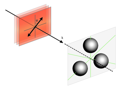
Fig.  1: Schematic view of the problem under consideration: linearly-polarised plane wave scattering by a system with rotational symmetry.

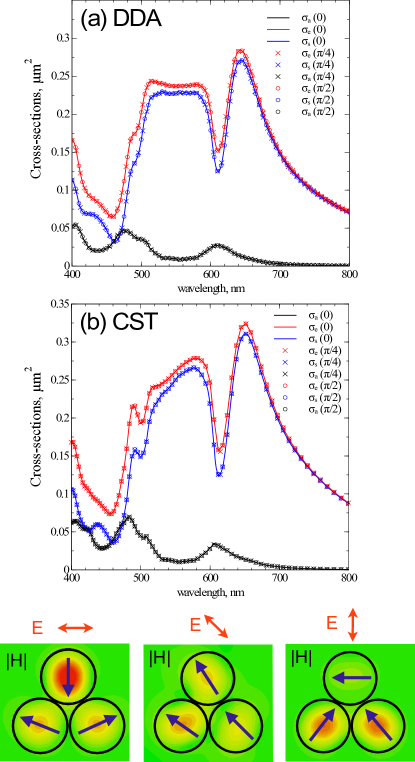
Fig.  2: Extinction, scattering and absorption cross-sections for three different polarisations of a trimer structure made of touching silicon nanopartices of radii $R=75$nm calculated by using (a) the discrete dipole approximation (DDA) method and (b) direct numerical simulations with CST Microwave Studio. Bottom panels show magnetic field distribution at the, $\lambda=612$nm, Fano resonance ⁴⁵ for all three polarisations together with the induced magnetic dipole moments.

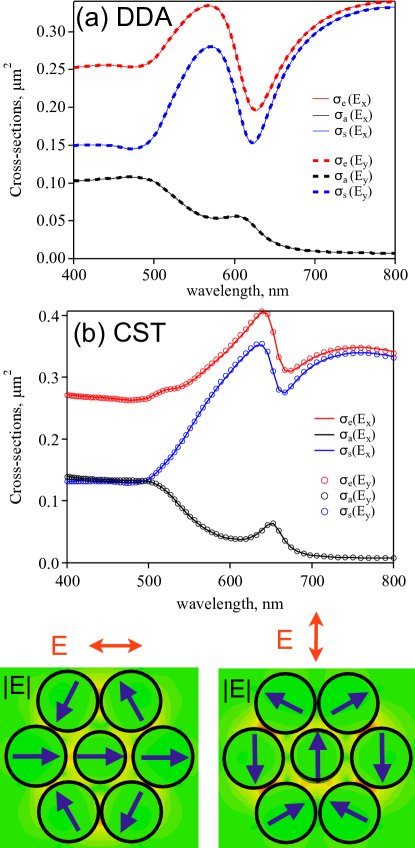
Fig.  3: Extinction, scattering and absorption cross-sections for two orthogonal polarisations of a heptamer structure made of gold nanopartices of central $R_{c}=65$nm and outer $R_{o}=75$nm radii separated by $d=10$nm calculated by using (a) the discrete dipole approximation (DDA) method and (b) direct numerical simulations with CST Microwave Studio. Bottom panels show electric field distribution at the, $\lambda=600$nm, Fano resonance ¹⁸ for two polarisations together with induced electric dipole moments.

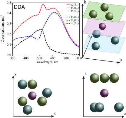
Fig.  4: Extinction, scattering and absorption cross-sections for a structure with 3-fold symmetry consisting of two equilateral trimers (marked by different colors) that are separated by a central particle and evenly spaced along the propagation axis, calculated by using the discrete dipole approximation (DDA). The trimers are additionally twisted with respect to each other in order to make the structure chiral and therefore satisfy only the minimum derived symmetry requirement needed to make the structure polarisation-independent.

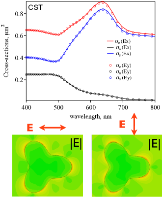
Fig.  5: Extinction, scattering and absorption cross-sections for two orthogonal polarisations of a continuous structure with 3-fold symmetry, calculated by using direct numerical simulations with CST Microwave Studio.

References

• Jun et al. 2009 Y. W. Jun, S. Sheikholeslami, D. R. Hostetter, C. Tajon, C. S. Craik and A. P. Alivisatos, P. Natl. Acad. Sci., 2009, 106, 17735.
• Liu et al. 2011 N. Liu, M. Hentschel, T. Weiss, A. P. Alivisatos and H. Giessen, Science, 2011, 332, 1407.
• Kabashin et al. 2009 A. V. Kabashin, P. Evans, S. Pastkovsky, W. Hendren, G. A. Wurtz, R. Atkinson, R. Pollard, V. A. Podolskiy and A. V. Zayats, Nat. Mater., 2009, 8, 867.
• Novotny and van Hulst 2011 L. Novotny and N. van Hulst, Nat. Photonics, 2011, 5, 83.
• Curto et al. 2010 A. G. Curto, G. Volpe, T. H. Taminiau, M. P. Kreuzer, R. Quidant and N. F. van Hulst, Science, 2010, 329, 930.
• Atwater and Polman 2010 H. A. Atwater and A. Polman, Nat. Mater., 2010, 9, 865.
• Bohren and Huffman 1983 C. F. Bohren and D. R. Huffman, Absorption and scattering of light by small particles, Wiley, New York, 1983, p. xiv.
• Kreibig and Vollmer 1995 U. Kreibig and M. Vollmer, Optical properties of metal clusters, Springer, Berlin ; New York, 1995.
• Ruan and Fan 2010 Z. C. Ruan and S. H. Fan, Phys. Rev. Lett., 2010, 105, 013901.
• Verslegers et al. 2012 L. Verslegers, Z. Yu, Z. Ruan, P. B. Catrysse and S. Fan, Phys. Rev. Lett., 2012, 108, 083902.
• Ni et al. 2012 X. J. Ni, N. K. Emani, A. V. Kildishev, A. Boltasseva and V. M. Shalaev, Science, 2012, 335, 427.
• Yu et al. 2011 N. F. Yu, P. Genevet, M. A. Kats, F. Aieta, J. P. Tetienne, F. Capasso and Z. Gaburro, Science, 2011, 334, 333.
• Noh et al. 2012 H. Noh, Y. Chong, A. D. Stone and H. Cao, Phys. Rev. Lett., 2012, 108, 186805.
• Miroshnichenko et al. 2010 A. E. Miroshnichenko, S. Flach and Y. S. Kivshar, Rev. Mod. Phys., 2010, 82, 2257.
• Luk’yanchuk et al. 2010 B. Luk’yanchuk, N. I. Zheludev, S. A. Maier, N. J. Halas, P. Nordlander, H. Giessen and C. T. Chong, Nat. Mater., 2010, 9, 707.
• Brandl et al. 2006 D. W. Brandl, N. A. Mirin and P. Nordlander, J. Phys. Chem. B, 2006, 110, 12302.
• Hao et al. 2008 F. Hao, Y. Sonnefraud, P. V. Dorpe, S. A. Maier, N. J. Halas and P. Nordlander, Nano Lett., 2008, 8, 3983.
• Hentschel et al. 2010 M. Hentschel, M. Saliba, R. Vogelgesang, H. Giessen, A. P. Alivisatos and N. Liu, Nano Lett., 2010, 10, 2721.
• Hentschel et al. 2011 M. Hentschel, D. Dregely, R. Vogelgesang, H. Giessen and N. Liu, ACS Nano, 2011, 5, 2042.
• King et al. 2011 N. S. King, Y. Li, C. Ayala-Orozco, T. Brannan, P. Nordlander and N. J. Halas, ACS Nano, 2011, 5, 7254.
• Ye et al. 2012 J. Ye, F. Wen, H. Sobhani, J. B. Lassiter, P. Dorpe, P. Nordlander and N. J. Halas, Nano Lett., 2012, 12, 1660.
• Frimmer et al. 2012 M. Frimmer, T. Coenen and A. F. Koenderink, Phys. Rev. Lett., 2012, 108, 077404.
• Evlyukhin et al. 2010 A. B. Evlyukhin, C. Reinhardt, A. Seidel, B. S. Luk’yanchuk and B. N. Chichkov, Phys. Rev. B., 2010, 82, 045404.
• Garcia-Etxarri et al. 2011 A. Garcia-Etxarri, R. Gomez-Medina, L. S. Froufe-Perez, C. Lopez, L. Chantada, F. Scheffold, J. Aizpurua, M. Nieto-Vesperinas and J. J. Saenz, Opt. Express, 2011, 19, 4815.
• Kuznetsov et al. 2012 A. I. Kuznetsov, A. E. Miroshnichenko, Y. H. Fu, J. B. Zhang and B. S. Lukyanchuk, Sci. Rep., 2012, 2, 492.
• Evlyukhin et al. 2012 A. B. Evlyukhin, S. M. Novikov, U. Zywietz, R. L. Eriksen, C. Reinhardt, S. I. Bozhevolnyi and B. N. Chichkov, Nano Lett., 2012, 12, 3749.
• Miroshnichenko et al. 2012 A. E. Miroshnichenko, B. Luk’yanchuk, S. A. Maier and Y. S. Kivshar, ACS Nano, 2012, 6, 837.
• Liu et al. 2012 W. Liu, A. E. Miroshnichenko, D. N. Neshev and Y. S. Kivshar, ACS Nano, 2012, 6, 5489.
• Liu et al. 2012 W. Liu, A. E. Miroshnichenko, D. N. Neshev and Y. S. Kivshar, Phys. Rev. B., 2012, 86, 081407.
• Rahmani et al. 2011 M. Rahmani, T. Tahmasebi, Y. Lin, B. Lukiyanchuk, T. Y. F. Liew and M. H. Hong, Nanotechnology, 2011, 22, 245204.
• Chuntonov and Haran 2011 L. Chuntonov and G. Haran, Nano Lett, 2011, 11, 2440.
• Shankar 1980 R. Shankar, Principles of quantum mechanics, Plenum Press, New York, 1980.
• Mcisaac 1975 P. R. Mcisaac, IEEE. T. Microw. Theory., 1975, 23, 429.
• Steel et al. 2001 M. J. Steel, T. P. White, C. M. de Sterke, R. C. McPhedran and L. C. Botten, Opt. Lett., 2001, 26, 488.
• Liu et al. 2010 W. Liu, A. A. Sukhorukov, A. E. Miroshnichenko, C. G. Poulton, Z. Y. Xu, D. N. Neshev and Y. S. Kivshar, Appl. Phys. Lett., 2010, 97, 021106.
• Aydin et al. 2011 K. Aydin, V. E. Ferry, R. M. Briggs and H. A. Atwater, Nat. Commun., 2011, 2, 517.
• Sheikholeslami et al. 2011 S. N. Sheikholeslami, A. Garcia-Etxarri and J. A. Dionne, Nano Lett., 2011, 11, 3927.
• Yurkin et al. 2010 M. A. Yurkin, D. De Kanter and A. G. Hoekstra, J. Nanophoton., 2010, 4, 041585.
• Alsawafta 2012 M. Alsawafta, Optical properties of metallic nanoparticles and metallic nanocomposite materials, 2012.
• McWeeny 1963 R. McWeeny, Symmetry: An introduction to group theory and its applications, Oergamon Pres, 1963.
• Cotton 1990 F. A. Cotton, Chemical Applications of Group Theory, 3rd edition, Wiley, 1990.
• Mulholland et al. 1994 G. W. Mulholland, C. F. Bohren and K. A. Fuller, Langmuir, 1994, 10, 2533.
• Palik 1997 E. D. Palik, Handbook of Optical Constants of Solids, Academic Press, 1997.
• Draine and Flatau 1994 B. T. Draine and P. J. Flatau, J. Opt. Soc. Am. A, 1994, 11, 1491–1499.
• Miroshnichenko and Kivshar 2012 A. E. Miroshnichenko and Y. S. Kivshar, Nano Lett., 2012, 12, 6459.
Refer to caption