Perturbative Non-Equilibrium Thermal Field Theory

Abstract

We present a new perturbative formulation of non-equilibrium thermal field theory, based upon non-homogeneous free propagators and time-dependent vertices. Our approach to non-equilibrium dynamics yields time-dependent diagrammatic perturbation series that are free of pinch singularities, without the need to resort to quasi-particle approximation or effective resummations of finite widths. In our formalism, the avoidance of pinch singularities is a consequence of the consistent inclusion of finite-time effects and the proper consideration of the time of observation. After arriving at a physically meaningful definition of particle number densities, we derive master time evolution equations for statistical distribution functions, which are valid to all orders in perturbation theory. The resulting equations do not rely upon a gradient expansion of Wigner transforms or involve any separation of time scales. To illustrate the key features of our formalism, we study out-of-equilibrium decay dynamics of unstable particles in a simple scalar model. In particular, we show how finite-time effects remove the pinch singularities and lead to violation of energy conservation at early times, giving rise to otherwise kinematically forbidden processes. The non-Markovian nature of the memory effects as predicted in our formalism is explicitly demonstrated.

I Introduction

As modern particle physics continues to advance at both the energy and intensity frontiers, we are increasingly concerned with transport phenomena in dense systems of ultra-relativistic particles, the so-called density frontier. One such system is the deconfined phase of quantum chromodynamics, known as the quark-gluon plasma Blaizot and Iancu (2002), whose existence has been inferred from the observation of jet quenching in Pb-Pb collisions by the ATLAS Aad et al. (2010), CMS Chatrchyan et al. (2011) and ALICE Aamodt et al. (2011) experiments at the CERN Large Hadron Collider (LHC). In addition to laboratory experiments, an understanding of such ultra-relativistic many-body dynamics is of interest in theoretical astro-particle physics and cosmology. Predictions about the evolution of the early Universe rely upon our understanding of the dynamics of states at the end and shortly after the phase of cosmological inflation.

The Wilkinson Microwave Anisotropy Probe (WMAP) Spergel et al. (2003, 2007) measured a baryon-to-photon ratio at the present epoch of ${\eta\>=\>n_{B}/n_{\gamma}\>=\>6.116^{+0.197}_{-0.249}\times 10^{-10}}$, where $n_{\gamma}$ is the number density of photons and ${n_{B}\>=\>n_{b}\>-\>n_{\bar{b}}}$ is the difference in number densities of baryons and anti-baryons. This observed Baryon Asymmetry of the Universe (BAU) is also consistent with the predictions of Big Bang Nucleosynthesis (BBN) Steigman (2005). The generation of the BAU requires the presence of out-of-equilibrium processes and the violation of baryon number ($B$), charge ($C$) and charge-parity ($CP$), according to the Sakharov conditions Sakharov (1967). One such set of processes is prescribed by the scenarios of baryogenesis via leptogenesis Kuzmin et al. (1985); Fukugita and Yanagida (1986, 1990), in which an initial excess in lepton number ($L$), provided by the decay of heavy right-handed Majorana neutrinos, is converted to a baryon number excess through the ${B+L}$-violating sphaleron interactions. The description of such phenomena require a consistent approach to the non-equilibrium dynamics of particle number densities. Further examples to which non-equilibrium approaches are relevant include, for instance, the phenomena of reheating and preheating Kofman et al. (1994); Boyanovsky et al. (1995); Baacke et al. (1997); Kofman et al. (1997) and the generation of dark matter relic densities Bender and Sarkar (2012).

The classical evolution of particle number densities in the early Universe is described by Boltzmann transport equations; see for instance Kolb and Wolfram (1980); Carena et al. (2003); Giudice et al. (2004); Pilaftsis and Underwood (2004); Buchmüller et al. (2005); Pilaftsis and Underwood (2005); Davidson et al. (2008); Deppisch and Pilaftsis (2011); Blanchet et al. (2013). A semi-classical improvement to these equations may be achieved by substituting the classical Boltzmann distributions with quantum-statistical Bose–Einstein and Fermi–Dirac distribution functions for bosons and fermions, respectively. However, such improved approaches take into account finite-width and off-shell effects by means of effective field-theoretic methods. Hence, a complete and systematic field-theoretic description of quantum transport phenomena would be desirable.

The first framework for calculating Ensemble Expectation Values (EEVs) of field operators was provided by Matsubara Matsubara (1955). This so-called Imaginary Time Formalism (ITF) of thermal field theory is derived by interpreting the canonical density operator as an evolution operator in negative imaginary time. Real-time Green’s functions may then be obtained by subtle analytic continuation. Nevertheless, the applicability of the ITF remains limited to the description of processes occurring in thermodynamic equilibrium.

The calculation of EEVs of operators in non-static systems is performed using the so-called Real Time Formalism (RTF); see for example Chou et al. (1985); Landsman and van Weert (1987). In particular, for non-equilibrium systems, one uses the Closed Time Path (CTP) formalism, or the in-in formalism, due to Schwinger and Keldysh Schwinger (1961); Keldysh (1964). The correspondence of these results with those obtained by the ITF in the equilibrium limit are discussed extensively in the literature Kobes (1990); Aurenche and Becherrawy (1992); Xu (1993); Baier and Niégawa (1994); Evans and Pearson (1995); van Eijck et al. (1994); Zhou (2002). A non-perturbative loopwise expansion of the CTP generating functional is then provided by the Cornwall–Jackiw–Tomboulis (CJT) effective action Cornwall et al. (1974); Carrington (2004), which was subsequently applied to the CTP formalism by Calzetta and Hu Calzetta and Hu (1987, 1988). The CJT effective action has been used extensively in applications to $1/N$ expansions far from equilibrium Aarts and Berges (2002); Aarts et al. (2002); Aarts and Martinez Resco (2003); Berges (2004); Arrizabalaga et al. (2004).

Recently, the computation of the out-of-equilibrium evolution of particle number densities has received much attention, where several authors put forward quantum-corrected or quantum Boltzmann equations Berera et al. (1998); Boyanovsky et al. (1998); Niegawa (1999); Cassing and Juchem (2000); Dadić (2000); Ivanov et al. (2000); Buchmuller and Fredenhagen (2000); Morawetz et al. (2001); Aarts and Berges (2001); Blaizot and Iancu (2002); Juchem et al. (2004); Prokopec et al. (2004a, b); Berges (2005); Arrizabalaga et al. (2005); Berges et al. (2005); Lindner and Müller (2006); Fillion-Gourdeau et al. (2006); De Simone and Riotto (2007); Cirigliano et al. (2008); Garbrecht and Konstandin (2009); Garny et al. (2010); Cirigliano et al. (2010); Beneke et al. (2011); Anisimov et al. (2011); Hamaguchi et al. (2012); Fidler et al. (2012); Gautier and Serreau (2012); Drewes et al. (2013). Existing approaches generally rely upon the Wigner transformation and gradient expansion Winter (1985); Bornath et al. (1996) of a system of Kadanoff–Baym (KB) Baym and Kadanoff (1961); Kadanoff and Baym (1989) equations, originally applied in the non-relativistic regime Danielewicz (1984); Lipavský et al. (1986); Rammer and Smith (1986); Bornath et al. (1996). Often the truncation of the gradient expansion is accompanied by quasi-particle ansaetze for the forms of the propagators. Similar approaches have recently been applied to the glasma Berges and Schlichting (2013). Dynamical equations have also been derived by expansion of the Liouville-von Neumann equation Sigl and Raffelt (1993); Gagnon and Shaposhnikov (2011) and using functional renormalization techniques Gasenzer et al. (2010).

In this article, we present a new approach to non-equilibrium thermal field theory. Our approach is based upon a diagrammatic perturbation series, constructed from non-homogeneous free propagators and time-dependent vertices, which encode the absolute space-time dependence of the thermal background. In particular, we show how the systematic inclusion of finite-time effects and the proper consideration of the time of observation render our perturbative expansion free of pinch singularities, thereby enabling a consistent treatment of non-equilibrium dynamics. Unlike other methods, our approach does not require the use of quasi-particle approximation or other effective resummations of finite-width effects.

A key element of our formalism has been to define physically meaningful particle number densities in terms of off-shell Green’s functions. This definition is unambiguous, as it can be closely linked to Noether’s charge, associated with a partially conserved current. Subsequently, we derive master time evolution equations for the statistical distribution functions related to particle number densities. These time evolution equations do not rely on the truncation of a gradient expansion of the so-called Wigner transforms; neither do they involve separation of various time scales. Instead, they are built of non-homogeneous free propagators, with modified time-dependent Feynman rules, which enable us to analyze the pertinent kinematics fully. Our analysis shows that the systematic inclusion of finite-time effects leads to the microscopic violation of energy conservation at early times. Aside from preventing the appearance of pinch singularities, the effect of a finite time interval of evolution leads to contributions from processes that would otherwise be kinematically disallowed on grounds of energy conservation. Applying this formalism to a simple scalar model with unstable particles, we show that these evanescent processes contribute significantly to the rapidly-oscillating transient evolution of these systems, inducing late-time memory effects. We find that the spectral evolution of two-point correlation functions exhibits an oscillating pattern with time-varying frequencies. Such an oscillating pattern signifies a non-Markovian evolution of memory effects, which is a distinctive feature governing truly out-of-thermal-equilibrium dynamical systems. A summary of the main results detailed in this article can be found in Millington and Pilaftsis (2013).

Table 1: Glossary for clarifying polysemous notation.

$T$	thermodynamic temperature
$t$	macroscopic time
$\tilde{t}$	microscopic real time
$\tau$	microscopic negative imaginary time
$\mathfrak{t}$	complex time
$\mathrm{T}$($\bar{\mathrm{T}}$)	time-(anti-time-)ordering operator
$\mathrm{T}_{\mathcal{C}}$	path-ordering operator
$Z$	wavefunction renormalization
$\mathcal{Z}$	partition function/ generating functional
$f$	statistical distribution function
$f_{\beta}$	Boltzmann distribution
$f_{\mathrm{B}}$	Bose–Einstein distribution
$\tilde{f}$	ensemble function
$\rho$	density operator/ density matrix
$n$	number density
$N$	total particle number

The outline of the paper is as follows. In Section II, we review the canonical quantization of a scalar field theory, placing particular emphasis on the inclusion of a finite time of coincidence for the three equivalent pictures of quantum mechanics, namely the Schrödinger, Heisenberg and Dirac (interaction) pictures. In Section III, we introduce the CTP formalism, limiting ourselves initially to consider its application to quantum field theory at zero temperature and density. This is followed by a discussion of the constraints upon the form of the CTP propagator. With these prerequisites reviewed, we proceed in Section IV to discuss the generalization of the CTP formalism to finite temperature and density in the presence of both spatially and temporally inhomogeneous backgrounds. In the same section, we derive the most general form of the non-homogeneous free propagators for a scalar field theory. The thermodynamic equilibrium limit is outlined in Section V. Subsequently, in Section VI, we define the concept of particle number density and relate this to a perturbative loopwise expansion of the resummed CTP propagators. In Section VII, we derive new master time evolution equations for statistical distribution functions, which go over to classical Boltzmann equations in the appropriate limits. In Section VIII, we demonstrate the absence of pinch singularities in the perturbation series arising in our approach at the one-loop level. Section IX studies the thermalization of unstable particles in a simple scalar model, where particular emphasis is laid on the early-time behavior and the impact of the finite-time effects. Finally, our conclusions and possible future directions are presented in Section X.

For clarity, a glossary that might be useful to the reader to clarify polysemous notation is given in Table 1. Appendix A provides a summary of all important propagator definitions, along with their basic relations and properties. In Appendix B, we describe the correspondence between the RTF and ITF in the equilibrium limit at the one-loop level for a real scalar field theory with a cubic self-interaction. The generalization of our approach to complex scalar fields is outlined in Appendix C. Appendix D contains a series expansion of the most general non-homogeneous Gaussian-like density operator. In Appendix E, we summarize the derivation of the so-called Kadanoff–Baym equations and their subsequent gradient expansion. Lastly, in Appendix F, we describe key technical details involved in the calculation of loop integrals with non-homogeneous free propagators.

II Canonical Quantization

In this section, we review the basic results obtained within the canonical quantization formalism for a massive scalar field theory. This discussion will serve as a precursor for our generalization to finite temperature and density, which follows in subsequent sections.

As a starting point, we consider a simple self-interacting theory of a real scalar field $\Phi(x)$ with mass $M$, which is described by the Lagrangian

$$\mathcal{L}(x)\ =\ \tfrac{1}{2}\partial_{\mu}\Phi(x)\partial^{\mu}\Phi(x)\>-\>\tfrac{1}{2}M^{2}\Phi^{2}(x)\>-\>\tfrac{1}{3!}g\Phi^{3}(x)\>-\>\tfrac{1}{4!}\lambda\Phi^{4}(x)\;,$$ (1)

where $g$ and $\lambda$ are dimensionful and dimensionless couplings, respectively. Throughout this article, we use the short-hand notation: $x\>\equiv\>x^{\mu}\>=\>(x^{0},\mathbf{x})$, for the four-dimensional space-time arguments of field operators, and adopt the signature $(+,-,-,-)$ for the Minkowski space-time metric $\eta_{\mu\nu}$.

It proves convenient to start our canonical quantization approach in the Schrödinger picture, where the state vectors are time dependent, whilst basis vectors and operators are, in the absence of external sources, time independent. Hence, the time-independent Schrödinger-picture field operator, denoted by a subscript $\mathrm{S}$, may be written in the familiar plane-wave decomposition

$$\Phi_{\mathrm{S}}(\mathbf{x};\tilde{t}_{i})\ =\ \int\!\mathrm{d}{\Pi_{\mathbf{p}}}\;\Big{(}\,a_{\mathrm{S}}(\mathbf{p};\tilde{t}_{i})e^{i\mathbf{p}\cdot\mathbf{x}}\>+\>a_{\mathrm{S}}^{{\dagger}}(\mathbf{p};\tilde{t}_{i})e^{-i\mathbf{p}\cdot\mathbf{x}}\,\Big{)}\;,$$ (2)

where we have introduced the short-hand notation:

$$\!\int\!\mathrm{d}{\Pi_{\mathbf{p}}}\ \equiv\ \!\int\!\!\frac{\mathrm{d}^{3}{\mathbf{p}}}{(2\pi)^{3}}\,\frac{1}{2E(\mathbf{p})}\ =\ \!\int\!\!\frac{\mathrm{d}^{4}{p}}{(2\pi)^{4}}\;2\pi\theta(p_{0})\delta(p^{2}-M^{2})\;,$$ (3)

for the Lorentz-invariant phase space (LIPS). In (3), $E(\mathbf{p})\>=\>\sqrt{\mathbf{p}^{2}+M^{2}}$ is the energy of the single-particle mode with three-momentum $\mathbf{p}$ and $\theta(p_{0})$ is the generalized unit step function, defined by the Fourier representation

$$\theta(p_{0})\ \equiv\ i\!\int_{-\infty}^{+\infty}\!\frac{\mathrm{d}{\xi}}{2\pi}\;\frac{e^{-ip_{0}\xi}}{\xi\>+\>i\epsilon}\ =\ \begin{cases}1\;,\qquad&p_{0}\ >\ 0\\ \frac{1}{2}\;,\qquad&p_{0}\ =\ 0\\ 0\;,\qquad&p_{0}\ <\ 0\;,\end{cases}$$ (4)

where $\epsilon=0^{+}$. It is essential to stress here that we define the Schrödinger-, Heisenberg- and Interaction (Dirac)-pictures to be coincident at the finite microscopic boundary time $\tilde{t}_{i}$, such that

$$\Phi_{\mathrm{S}}(\mathbf{x};\tilde{t}_{i})\ =\ \Phi_{\mathrm{H}}(\tilde{t}_{i},\mathbf{x};\tilde{t}_{i})\ =\ \Phi_{\mathrm{I}}(\tilde{t}_{i},\mathbf{x};\tilde{t}_{i})\;,$$ (5)

where implicit dependence upon the boundary time $\tilde{t}_{i}$ is marked by separation from explicit arguments by a semi-colon.

The time-independent Schrödinger-picture operators $a_{\mathrm{S}}^{{\dagger}}(\mathbf{p};\tilde{t}_{i})$ and $a_{\mathrm{S}}(\mathbf{p};\tilde{t}_{i})$ are the usual creation and annihilation operators, which act on the stationary vacuum $\ket{0}$, respectively creating and destroying time-independent single-particle momentum eigenstates. Their defining properties are:

$$a_{\mathrm{S}}^{{\dagger}}(\mathbf{p};\tilde{t}_{i})\!\ket{0} \ =\ \ket{\mathbf{p};\tilde{t}_{i}}\!\;,$$ (6a)

$$a_{\mathrm{S}}(\mathbf{p};\tilde{t}_{i})\!\ket{\mathbf{p}^{\prime};\tilde{t}_{i}} \ =\ (2\pi)^{3}2E(\mathbf{p})\delta^{(3)}(\mathbf{p}\>-\>\mathbf{p}^{\prime})\!\ket{0}\!\;,$$ (6b)

$$a_{\mathrm{S}}(\mathbf{p};\tilde{t}_{i})\!\ket{0} \ =\ 0\;.$$ (6c)

Note that the momentum eigenstates $\ket{\mathbf{p};\tilde{t}_{i}}$ respect the orthonormality condition

$$\braket{\mathbf{p}^{\prime};\tilde{t}_{i}}{\mathbf{p};\tilde{t}_{i}}\ =\ (2\pi)^{3}2E(\mathbf{p})\delta^{(3)}(\mathbf{p}\>-\>\mathbf{p}^{\prime})\;.$$ (7)

We then define the time-dependent interaction-picture field operator $\Phi_{\mathrm{I}}(x;\tilde{t}_{i})$ via

$$\Phi_{\mathrm{I}}(x;\tilde{t}_{i})\ =\ e^{iH_{\mathrm{S}}^{0}(x_{0}\>-\>\tilde{t}_{i})}\Phi_{\mathrm{S}}(\mathbf{x};\tilde{t}_{i})e^{-iH_{\mathrm{S}}^{0}(x_{0}\>-\>\tilde{t}_{i})}\;,$$ (8)

where $H_{\mathrm{S}}^{0}$ is the free part of the Hamiltonian in the Schrödinger picture. Using the commutators

$$\big{[}\,H_{\mathrm{S}}^{0},\>a_{\mathrm{S}}(\mathbf{p};\tilde{t}_{i})\,\big{]} \ =\ -E(\mathbf{p})a_{\mathrm{S}}(\mathbf{p};\tilde{t}_{i})\;,$$ (9a)

$$\big{[}\,H_{\mathrm{S}}^{0},\>a^{{\dagger}}_{\mathrm{S}}(\mathbf{p};\tilde{t}_{i})\,\big{]} \ =\ +E(\mathbf{p})a^{{\dagger}}_{\mathrm{S}}(\mathbf{p};\tilde{t}_{i})\;,$$ (9b)

the interaction-picture field operator may be written

$$\Phi_{\mathrm{I}}(x;\tilde{t}_{i})\ =\ \int\!\mathrm{d}{\Pi_{\mathbf{p}}}\,\Big{(}\,a_{\mathrm{S}}(\mathbf{p};\tilde{t}_{i})e^{-iE(\mathbf{p})(x_{0}\>-\>\tilde{t}_{i})}e^{i\mathbf{p}\cdot\mathbf{x}}\>+\>a_{\mathrm{S}}^{{\dagger}}(\mathbf{p};\tilde{t}_{i})e^{iE(\mathbf{p})(x_{0}\>-\>\tilde{t}_{i})}e^{-i\mathbf{p}\cdot\mathbf{x}}\,\Big{)}\;,$$ (10)

or equivalently, in terms of interaction-picture operators only,

$$\Phi_{\mathrm{I}}(x;\tilde{t}_{i})\ =\ \!\int\!\mathrm{d}{\Pi_{\mathbf{p}}}\;\Big{(}\,a_{\mathrm{I}}(\mathbf{p},0;\tilde{t}_{i})e^{-iE(\mathbf{p})x_{0}}e^{i\mathbf{p}\cdot\mathbf{x}}\>+\>a_{\mathrm{I}}^{{\dagger}}(\mathbf{p},0;\tilde{t}_{i})e^{iE(\mathbf{p})x_{0}}e^{-i\mathbf{p}\cdot\mathbf{x}}\,\Big{)}\;.$$ (11)

Notice that in (11) the time-dependent interaction-picture creation and annihilation operators, $a_{\mathrm{I}}^{\dagger}(\mathbf{p},\tilde{t};\tilde{t}_{i})$ and $a_{\mathrm{I}}(\mathbf{p},\tilde{t};\tilde{t}_{i})$, are evaluated at the microscopic time $\tilde{t}\>=\>0$, after employing a relation analogous to (8). We may write the four-dimensional Fourier transform of the interaction-picture field operator as

$$\Phi_{\mathrm{I}}(p;\tilde{t}_{i})\ =\ \!\int\!\mathrm{d}^{4}{x}\;e^{ip\cdot x}\,\Phi_{\mathrm{I}}(x;\tilde{t}_{i})\ =\ 2\pi\delta(p^{2}-M^{2})\Big{(}\,\theta(p_{0})a_{\mathrm{I}}(\mathbf{p},0;\tilde{t}_{i})\>+\>\theta(-p_{0})a^{{\dagger}}_{\mathrm{I}}(-\mathbf{p},0;\tilde{t}_{i})\,\Big{)}\;.$$ (12)

In the limit where the interactions are switched off adiabatically as $\tilde{t}_{i}\>\to\>-\infty$, one may define the asymptotic in creation and annihilation operators via

$$a^{({\dagger})}_{\mathrm{in}}(\mathbf{p})\ \simeq\ Z^{-1/2}\lim_{\tilde{t}_{i}\>\to\>-\infty}a^{({\dagger})}_{\mathrm{I}}(\mathbf{p},0;\tilde{t}_{i})\ =\ Z^{-1/2}\lim_{\tilde{t}_{i}\>\to\>-\infty}a^{({\dagger})}_{\mathrm{S}}(\mathbf{p};\tilde{t}_{i})e^{+(-)iE(\mathbf{p})\tilde{t}_{i}}\;,$$ (13)

where $Z\>=\>1\>+\>\mathcal{O}(\hbar)$ is the wavefunction renormalization. Evidently, keeping track of the finite boundary time $\tilde{t}_{i}$ plays an important role in ensuring that our forthcoming generalization to perturbative thermal field theory remains consistent with asymptotic field theory in the limit $\tilde{t}_{i}\>\to\>-\infty$. Hereafter, we will omit the subscript $\mathrm{I}$ on interaction-picture operators and suppress the implicit dependence on the boundary time $\tilde{t}_{i}$, except where it is necessary to do otherwise for clarity.

We start our quantization procedure by defining the commutator of interaction-picture fields

$$\big{[}\,\Phi(x),\>\Phi(y)\,\big{]}\ \equiv\ i\Delta^{0}(x,y;M^{2})\;,$$ (14)

where $i\Delta^{0}(x,y;M^{2})$ is the free Pauli-Jordan propagator. Herein, we denote free propagators by a superscript $0$. The condition of micro-causality requires that the interaction-picture fields commute for space-like separations $(x\>-\>y)^{2}\><\>0$. This restricts $i\Delta^{0}(x,y;M^{2})$ to be invariant under spatial translations, having the Poincaré-invariant form

$$i\Delta^{0}(x,y;M^{2})\ =\ \!\int\!\mathrm{d}{\Pi_{\mathbf{p}}}\;\Big{(}\,e^{-iE(\mathbf{p})(x^{0}\>-\>y^{0})}e^{i\mathbf{p}\cdot(\mathbf{x}\>-\>\mathbf{y})}\>-\>\big{(}\,x\>\longleftrightarrow\>y\,\big{)}\,\Big{)}\;.$$ (15)

Observe that $i\Delta^{0}(x,y;M^{2})$ represents the difference of two counter-propagating packets of plane waves and vanishes for $(x\>-\>y)^{2}\><\>0$.

It proves useful for our forthcoming analysis to introduce the double Fourier transform

$$i\Delta^{0}(p,p^{\prime};M^{2}) \ =\ \!\iint\!\mathrm{d}^{4}{x}\,\mathrm{d}^{4}{y}\;e^{ip\cdot x}e^{-ip^{\prime}\cdot y}\,i\Delta^{0}(x,y;M^{2})$$ (16a)

$$\ =\ 2\pi\varepsilon(p_{0})\delta(p^{2}-M^{2})(2\pi)^{4}\delta^{(4)}(p\>-\>p^{\prime})\;,$$ (16b)

where $\varepsilon(p_{0})\>\equiv\>\theta(p_{0})\>-\>\theta(-p_{0})$ is the generalized signum function. Note that we have defined the Fourier transforms such that four-momentum $p$ flows away from the point $x$ and four-momentum $p^{\prime}$ flows towards the point $y$.

From (14) and (15), we may derive the equal-time commutation relations

$$i\Delta^{0}(x,y;M^{2})\big{|}_{x^{0}\>=\>y^{0}\>=\>\tilde{t}} \ =\ \big{[}\,\Phi(\tilde{t},\mathbf{x}),\>\Phi(\tilde{t},\mathbf{y})\,\big{]}\ =\ 0\;,$$ (17a)

$$\partial_{x_{0}}i\Delta^{0}(x,y;M^{2})\big{|}_{x^{0}\>=\>y^{0}\>=\>\tilde{t}} \ =\ \big{[}\,\pi(\tilde{t},\mathbf{x}),\>\Phi(\tilde{t},\mathbf{y})\,\big{]}\ =\ -i\delta^{(3)}(\mathbf{x}\>-\>\mathbf{y})\;,$$ (17b)

$$\partial_{x_{0}}\partial_{y_{0}}i\Delta^{0}(x,y;M^{2})\big{|}_{x^{0}\>=\>y^{0}\>=\>\tilde{t}} \ =\ \big{[}\,\pi(\tilde{t},\mathbf{x}),\>\pi(\tilde{t},\mathbf{y})\,\big{]}\ =\ 0\;,$$ (17c)

where $\pi(x)\>=\>\partial_{x_{0}}\Phi(x)$ is the conjugate-momentum operator. In order to satisfy the canonical quantization relations (17), the creation and annihilation operators must respect the commutation relation

$$\big{[}\,a(\mathbf{p},\tilde{t}\,),\>a^{{\dagger}}(\mathbf{p}^{\prime},\tilde{t}^{\prime}\,)\,\big{]}\ =\ (2\pi)^{3}2E(\mathbf{p})\delta^{(3)}(\mathbf{p}\>-\>\mathbf{p}^{\prime})e^{-iE(\mathbf{p})(\tilde{t}\>-\>\tilde{t}^{\prime})}\;,$$ (18)

with all other commutators vanishing. Here, we emphasize the appearance of an overall phase $e^{-iE(\mathbf{p})(\tilde{t}\>-\>\tilde{t}^{\prime})}$ in (18) for $\tilde{t}\>\neq\>\tilde{t}^{\prime}$ [cf. Section IV.1].

The vacuum expectation value of the commutator of Heisenberg-picture field operators may be expressed as a superposition of interaction-picture field commutators by means of the Källén–Lehmann spectral representation Källén (1952); Lehmann (1954):

$$\braket{0}{\big{[}\,\Phi_{\mathrm{H}}(x),\;\Phi_{\mathrm{H}}(y)\,\big{]}}{0}\ \equiv\ i\Delta(x,y)\ =\ \!\int_{0}^{\infty}\!\!\mathrm{d}{s}\;\sigma(s)\,i\Delta^{0}(x,y;s)\;,$$ (19)

where $i\Delta^{0}(x,y;s)$ is the free Pauli–Jordan propagator in (15) with $M^{2}$ replaced by $s$ and $i\Delta(x,y)$ is the dressed or resummed propagator. The positive spectral density $\sigma(s)$ contains all information about the spectrum of single- and multi-particle states produced by the Heisenberg-picture field operators $\Phi_{\mathrm{H}}$. Note that for a homogeneous and stationary vacuum $\ket{0}$, $\sigma(s)$ is independent of the space-time coordinates and the resummed Pauli–Jordan propagator maintains its translational invariance. If $\sigma(s)$ is normalized, such that

$$\int_{0}^{\infty}\!\!\mathrm{d}{s}\;\sigma(s)\ =\ 1\;,$$ (20)

the equal-time commutation relations of Heisenberg-picture operators maintain exactly the form in (17). In this case, the spectral function cannot depend upon any fluctuations in the background. Clearly, for non-trivial ‘vacua’, or thermal backgrounds, the spectral density becomes a function also of the coordinates. The spectral representation of the resummed propagators may then depend non-trivially on space-time coordinates, i.e. $\sigma\>=\>\sigma(s;x,y)$; see for instance Aarts and Berges (2001). In this case, the convenient factorization of the Källén–Lehmann representation breaks down.

The retarded and advanced causal propagators are defined as

$$i\Delta_{\mathrm{R}}(x,y)\ \equiv\ \theta(x_{0}\>-\>y_{0})i\Delta(x,y)\;,\qquad i\Delta_{\mathrm{A}}(x,y)\ \equiv\ -\theta(y_{0}\>-\>x_{0})i\Delta(x,y)\;.$$ (21)

Using the Fourier representation of the unit step function in (4), we introduce a convenient representation of these causal propagators in terms of the convolution

$$i\Delta_{\mathrm{R}(\mathrm{A})}(p,p^{\prime})\ =\ i\!\int\!\frac{\mathrm{d}{k_{0}}}{2\pi}\;\frac{i\Delta(p_{0}-k_{0},p_{0}^{\prime}-k_{0};\mathbf{p},\mathbf{p}^{\prime})}{k_{0}\>+(-)\>i\epsilon}\;.$$ (22)

The absolutely-ordered Wightman propagators are defined as

$$i\Delta_{>}(x,y)\ \equiv\ \braket{\,\Phi(x)\Phi(y)\,}\!\;,\qquad i\Delta_{<}(x,y)\ \equiv\ \braket{\,\Phi(y)\Phi(x)\,}\!\;.$$ (23)

We note that the two-point correlation functions $\Delta(x,y)$, $\Delta_{>,<}(x,y)$ and $\Delta_{\rm R,A}(x,y)$ satisfy the causality relation:

$$\Delta(x,y)\ =\ \Delta_{>}(x,y)\>-\>\Delta_{<}(x,y)\ =\ \Delta_{\mathrm{R}}(x,y)\>-\>\Delta_{\mathrm{A}}(x,y)\;.$$ (24)

Our next step is to define the non-causal Hadamard propagator, which is the vacuum expectation value of the field anti-commutator

$$i\Delta_{1}(x,y)\ \equiv\ \braket{\,\big{\{}\,\Phi(x),\>\Phi(y)\,\big{\}}\,}\!\;.$$ (25)

Correspondingly, the time-ordered Feynman and anti-time-ordered Dyson propagators are given by

$$i\Delta_{\mathrm{F}}(x,y)\ \equiv\ \braket{\,\mathrm{T}\,\big{[}\,\Phi(x)\Phi(y)\,\big{]}\,}\!\;,\qquad i\Delta_{\mathrm{D}}(x,y)\ \equiv\ \braket{\bar{\,\mathrm{T}}\,\big{[}\,\Phi(x)\Phi(y)\,\big{]}\,}\!\;,$$ (26)

where $\mathrm{T}$ and $\bar{\mathrm{T}}$ are the time- and anti-time-ordering operators, respectively. Explicitly, $\Delta_{\mathrm{F}}(x,y)$ and $\Delta_{\mathrm{D}}(x,y)$ may be written in terms of the absolutely-ordered Wightman propagators $\Delta_{>}(x,y)$ and $\Delta_{<}(x,y)$ as

$$\Delta_{\mathrm{F}}(x,y)\ =\ \theta(x_{0}\>-\>y_{0})\Delta_{>}(x,y)\>+\>\theta(y_{0}\>-\>x_{0})\Delta_{<}(x,y)\;,$$ (27a)

$$\Delta_{\mathrm{D}}(x,y)\ =\ \theta(x_{0}\>-\>y_{0})\Delta_{<}(x,y)\>+\>\theta(y_{0}\>-\>x_{0})\Delta_{>}(x,y)\;.$$ (27b)

The propagators $\Delta_{1}(x,y)$, $\Delta_{>,<}(x,y)$ and $\Delta_{\rm F,D}(x,y)$ obey the unitarity relations:

$$\Delta_{1}(x,y)\ =\ \Delta_{\mathrm{F}}(x,y)\>+\>\Delta_{\mathrm{D}}(x,y)\ =\ \Delta_{>}(x,y)\>+\>\Delta_{<}(x,y)\ =\ 2i\mathrm{Im}\,\Delta_{\mathrm{F}}(x,y)\;.$$ (28)

Finally, for completeness, we define the principal-part propagator

$$\Delta_{\mathcal{P}}(x,y)\ =\ \frac{1}{2}\Big{(}\,\Delta_{\mathrm{R}}(x,y)\>+\>\Delta_{\mathrm{A}}(x,y)\,\Big{)}\ =\ \mathrm{Re}\,\Delta_{\mathrm{F}}(x,y)\;.$$ (29)

Here, we should bear in mind that

$$\mathrm{Re}\big{(}\mathrm{Im}\big{)}\,\Delta_{\mathrm{F}}(x,y)\ \neq\ \!\iint\!\!\frac{\mathrm{d}^{4}{p}}{(2\pi)^{4}}\;\frac{\mathrm{d}^{4}{p^{\prime}}}{(2\pi)^{4}}\,e^{-ip\cdot x}e^{ip^{\prime}\cdot y}\,\mathrm{Re}\big{(}\mathrm{Im}\big{)}\,\Delta_{\mathrm{F}}(p,p^{\prime})\;,$$ (30)

implying that

$$\Delta_{\mathcal{P}}(p,p^{\prime})\ \neq\ \mathrm{Re}\,\Delta_{\mathrm{F}}(p,p^{\prime})\;,$$ (31)

unless $\Delta_{\mathrm{F}}(p,p^{\prime})\>=\>\Delta_{\mathrm{F}}(-p,-p^{\prime})$, which is not generally true in non-equilibrium thermal field theory [cf. (322f)].

The definitions and the relations discussed above are valid for both free and resummed propagators. In Appendix A, we list the properties of these propagators in coordinate, momentum and Wigner (see Section IV.2) representations, as well as a number of useful identities, which we will refer to throughout this article. More detailed discussion related to these propagators and their contour-integral representations may be found in Greiner and Reinhardt (1996). In Appendix C, these considerations and the analysis of the following sections are generalized to the complex scalar field.

III The CTP Formalism

In this section, we review the Closed Time Path (CTP) formalism, or the so-called in-in formalism, due to Schwinger and Keldysh Schwinger (1961); Keldysh (1964). As an illuminating exercise, we consider the CTP formalism in the context of zero-temperature quantum field theory and derive the associated $2\times 2$ matrix propagator, obeying basic field-theoretic constraints, such as $CPT$ invariance, Hermiticity, causality and unitarity. Finally, we discuss the properties of the resummed propagator in the CTP formalism.

In the calculation of scattering-matrix elements, we are concerned with the transition amplitude between in and out asymptotic states, where single-particle states are defined in the infinitely-distant past and future. On the other hand, in quantum statistical mechanics, we are interested in the calculation of Ensemble Expectation Values (EEVs) of operators at a fixed given time $t$. Specifically, the evaluation of EEVs of operators requires a field-theoretic approach that allows us to determine the transition amplitude between states evolved to the same time. This approach is the Schwinger–Keldysh CTP formalism, which we describe in detail below.

For illustration, let us consider the following observable ${\cal O}$ in the Schrödinger picture (suppressing the spatial coordinates $\mathbf{x}$ and $\mathbf{y}$):

$${\cal O}_{\rm(S)}(\tilde{t}_{f};\tilde{t}_{i})\ =\ \!\int\![\mathrm{d}{\Phi(\mathbf{z})}]\;\prescript{}{\mathrm{S}}{\braket{\Phi(\mathbf{z}),\tilde{t}_{f};\tilde{t}_{i}}{\Phi_{\mathrm{S}}(\mathbf{x};\tilde{t}_{i})\Phi_{\mathrm{S}}(\mathbf{y};\tilde{t}_{i})}{\Phi(\mathbf{z}),\tilde{t}_{f};\tilde{t}_{i}}}_{\mathrm{S}}\;,$$ (32)

where $[\mathrm{d}{\Phi}]$ represents the functional integral over all field configurations $\Phi(\mathbf{z})$. In (32), $\ket{\Phi(\mathbf{z}),\tilde{t}_{f};\tilde{t}_{i}}_{\mathrm{S}}$ is a time-evolved eigenstate of the time-independent Schrödinger-picture field operator $\Phi_{\mathrm{S}}(\mathbf{x};\tilde{t}_{i})$ with eigenvalue $\Phi(\mathbf{x})$ at time $\tilde{t}_{f}\>=\>\tilde{t}_{i}$, where the implicit dependence upon the boundary time $\tilde{t}_{i}$ has been restored.

We should remark here that there are seven independent space-time coordinates involved in the observable (32). These are the six spatial coordinates, $\mathbf{x}$ and $\mathbf{y}$, plus the microscopic time $\tilde{t}_{f}$. In addition, there is one implicit coordinate: the boundary time $\tilde{t}_{i}$. As we will see, exactly seven independent coordinates are required to construct physical observables that are compatible with Heisenberg’s uncertainty principle. We choose the seven independent coordinates to be

$$t\ =\ \tilde{t}_{f}\>-\>\tilde{t}_{i}\;,\qquad\mathbf{X}\ =\ \frac{1}{2}\>\Big{(}\mathbf{x}\>+\>\mathbf{y}\Big{)}\;,\qquad\mathbf{p}\;,$$ (33)

where $t$ and $\mathbf{X}$ are the macroscopic time and central space coordinates and $\mathbf{p}$ is the Fourier-conjugate variable to the relative spatial coordinate $\mathbf{R}\>=\>\mathbf{x}\>-\>\mathbf{y}$.

In the interaction picture, the same observable ${\cal O}$ in (32) is given by

$${\cal O}_{\rm(I)}(\tilde{t}_{f};\tilde{t}_{i})\ =\ \!\int\![\mathrm{d}{\Phi(\mathbf{z})}]\;\prescript{}{\mathrm{I}}{\braket{\Phi(\mathbf{z}),\tilde{t}_{f};\tilde{t}_{i}}{\Phi_{\mathrm{I}}(\tilde{t}_{f},\mathbf{x};\tilde{t}_{i})\Phi_{\mathrm{I}}(\tilde{t}_{f},\mathbf{y};\tilde{t}_{i})}{\Phi(\mathbf{z}),\tilde{t}_{f};\tilde{t}_{i}}}_{\mathrm{I}}\;;$$ (34)

and, in the Heisenberg picture, by

$${\cal O}_{\rm(H)}(\tilde{t}_{f};\tilde{t}_{i})\ =\ \int\![\mathrm{d}{\Phi(\mathbf{z})}]\;\prescript{}{\mathrm{H}}{\braket{\Phi(\mathbf{z});\tilde{t}_{i}}{\Phi_{\mathrm{H}}(\tilde{t}_{f},\mathbf{x};\tilde{t}_{i})\Phi_{\mathrm{H}}(\tilde{t}_{f},\mathbf{y};\tilde{t}_{i})}{\Phi(\mathbf{z});\tilde{t}_{i}}}_{\mathrm{H}}\;.$$ (35)

Notice that the prediction for the observable ${\cal O}$ does not depend on which picture we are using, i.e. ${\cal O}_{\rm(S)}(\tilde{t}_{f};\tilde{t}_{i})\>=\>{\cal O}_{\rm(I)}(\tilde{t}_{f};\tilde{t}_{i})\>=\>{\cal O}_{\rm(H)}(\tilde{t}_{f};\tilde{t}_{i})$. This picture independence of ${\cal O}$ is only possible because the time-dependent vectors and operators in ${\cal O}$ are evaluated individually at equal times. Otherwise, any potential observable, built out of time-dependent vectors and operators that are evaluated at different times, would be picture dependent and therefore unphysical. Moreover, the prediction of the observable $\mathcal{O}$ should be invariant under simultaneous time translations of the boundary and observation times, $\tilde{t}_{i}$ and $\tilde{t}_{f}$, i.e.

$$\mathcal{O}(\tilde{t}_{f};\tilde{t}_{i})\ =\ \mathcal{O}(t;0)\ \equiv\ \mathcal{O}(t),$$ (36)

where $t\>=\>\tilde{t}_{f}\>-\>\tilde{t}_{i}$ is the macroscopic time, as we will see below. Herein and throughout the remainder of this article, the time arguments of quantities that are invariant under such simultaneous translations of the boundary times are written in terms of the macroscopic time $t$ only.

III.1 The CTP Contour

In order to evaluate equal-time observables of the form in (35), we first introduce the in vacuum state $\ket{0_{\mathrm{in}};\tilde{t}_{i}}$, which is at time $\tilde{t}_{i}$ a time-independent eigenstate of the Heisenberg field operator $\Phi_{\mathrm{H}}(x;\tilde{t}_{i})$ with zero eigenvalue; see Calzetta and Hu (1987, 1988). We then need a means of driving the amplitude $\braket{0_{\mathrm{in}};\tilde{t}_{i}}{0_{\mathrm{in}};\tilde{t}_{i}}$, which can be achieved by the appropriate introduction of external sources.

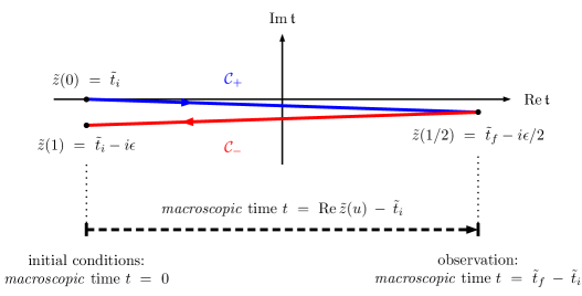
Figure 1: The closed-time path, $\mathcal{C}\ =\ \mathcal{C}_{+}\>\cup\,\>\mathcal{C}_{-}$, running first along $\mathcal{C}_{+}$ from $\tilde{t}_{i}$ to $\tilde{t}_{f}\>-\>i\epsilon/2$ and then returning along $\mathcal{C}_{-}$ from $\tilde{t}_{f}\>-\>i\epsilon/2$ to $\tilde{t}_{i}\>-\>i\epsilon$. The relationship between the complex microscopic time $\tilde{z}(u)$ and the macroscopic time $t$ is indicated by a dashed black arrow.

The procedure may be outlined with the aid of Figure 1 as follows. We imagine evolving our in state at time $\tilde{t}_{i}$ forwards in time under the influence of a source $J_{+}(x)$ to some out state at time $\tilde{t}_{f}$ in the future, which will be a superposition over all possible future states. We then evolve this superposition of states backwards again under the influence of a second source $J_{-}(x)$, returning to the same initial time $\tilde{t}_{i}$ and the original in state. The sources $J_{\pm}(x)$ are assumed to vanish adiabatically at the boundaries of the interval $[\tilde{t}_{i},\ \tilde{t}_{f}]$. We may interpret the path of this evolution as defining a closed contour  $\mathcal{C}\>=\>\mathcal{C}_{+}\>\cup\,\>\mathcal{C}_{-}$ in the complex-time plane ($\mathfrak{t}$-plane, $\mathfrak{t}\>\in\>\mathbb{C}$), which is the union of two anti-parallel branches: $\mathcal{C}_{+}$, running from $\tilde{t}_{i}$ to $\tilde{t}_{f}\>-\>i\epsilon/2$; and $\mathcal{C}_{-}$, running from $\tilde{t}_{f}\>-\>i\epsilon/2$ back to $\tilde{t}_{i}\>-\>i\epsilon$. We refer to $\mathcal{C}_{+}$ and $\mathcal{C}_{-}$ as the positive time-ordered and negative anti-time-ordered branches, respectively. As depicted in Figure 1, the small imaginary part $\epsilon\>=\>0^{+}$ has been added to allow us to distinguish the two, essentially coincident, branches. We parametrize the distance along the contour, starting from $\tilde{t}_{i}$, by the real variable $u\>\in\>[0,\ 1]$, which increases monotonically along $\mathcal{C}$. We may then define the contour by a path $\tilde{z}(u)\>=\>\tilde{t}(u)\>-\>i\tilde{\tau}(u)\>\in\>\mathfrak{t}$, where $\tilde{t}(0)\>=\>\tilde{t}(1)\>=\>\tilde{t}_{i}$ and $\tilde{t}(1/2)\>=\>\tilde{t}_{f}$. Thus, the complex CTP contour $\tilde{z}(u)$ may be written down explicitly as

$$\tilde{z}(u)\ =\ \theta(\tfrac{1}{2}-u)\,\Big{[}\,\tilde{t}_{i}\>+\>2u\,\big{(}\,\tilde{t}_{f}\>-\>\tilde{t}_{i}\,\big{)}\,\Big{]}\>+\>\theta(u-\tfrac{1}{2})\,\Big{[}\,\tilde{t}_{i}\>+\>2\,\big{(}\,1\>-\>u\,\big{)}\,\big{(}\,\tilde{t}_{f}\>-\>\tilde{t}_{i}\,\big{)}\,\Big{]}\>-\>i\epsilon u\;,$$ (37)

with $\theta(0)\>=\>1/2$, as given in (4).

To derive a path-integral representation of the generating functional, we introduce the eigenstate $\ket{\Phi(\mathbf{x}),\tilde{t};\tilde{t}_{i}}$ of the Heisenberg field operator $\Phi_{\mathrm{H}}(\tilde{t},\mathbf{x};\tilde{t}_{i})$, satisfying the eigenvalue equation

$$\Phi_{\mathrm{H}}(\tilde{t},\mathbf{x};\tilde{t}_{i})\!\ket{\Phi(\mathbf{x}),\tilde{t};\tilde{t}_{i}}\ =\ \Phi(\mathbf{x})\!\ket{\Phi(\mathbf{x}),\tilde{t};\tilde{t}_{i}}\;.$$ (38)

The basis vectors $\ket{\Phi(\mathbf{x}),\tilde{t};\tilde{t}_{i}}$ form a complete orthonormal basis, respecting the orthonormality condition

$$\int\![\mathrm{d}{\Phi(\mathbf{x})}]\;\ket{\Phi(\mathbf{x}),\tilde{t};\tilde{t}_{i}}\bra{\Phi(\mathbf{x}),\tilde{t};\tilde{t}_{i}}\ =\ \mathbb{I}\;.$$ (39)

We may then write the CTP generating functional $\mathcal{Z}[J_{\pm},t]$ as

$$\mathcal{Z}[J_{\pm},t] \ =\ \!\int\![\mathrm{d}{\Phi(\mathbf{x})}]\;\prescript{}{J_{-}}{\braket{0_{\mathrm{in}},\tilde{t}_{i};\tilde{t}_{i}}{\Phi(\mathbf{x}),\tilde{t}_{f};\tilde{t}_{i}}}\braket{\Phi(\mathbf{x}),\tilde{t}_{f};\tilde{t}_{i}}{0_{\mathrm{in}},\tilde{t}_{i};\tilde{t}_{i}}_{J_{+}}$$

$$\ =\ \!\int\![\mathrm{d}{\Phi(\mathbf{x})}]\;\braket{0_{\mathrm{in}},\tilde{t}_{i};\tilde{t}_{i}}{\,\bar{\mathrm{T}}\,\Big{(}\,e^{-i\int_{\tilde{t}_{i}}^{\tilde{t}_{f}}\!\mathrm{d}^{4}{x}\;J_{-}(x)\Phi_{\mathrm{H}}(x)}\,\Big{)}}{\Phi(\mathbf{x}),\tilde{t}_{f};\tilde{t}_{i}}$$

$$\hskip 51.21504pt\times\braket{\Phi(\mathbf{x}),\tilde{t}_{f};\tilde{t}_{i}}{\,\mathrm{T}\,\Big{(}\,e^{i\int_{\tilde{t}_{i}}^{\tilde{t}_{f}}\!\mathrm{d}^{4}{x}\;J_{+}(x)\Phi_{\mathrm{H}}(x)}\,\Big{)}}{0_{\mathrm{in}},\tilde{t}_{i};\tilde{t}_{i}}\;,$$ (40)

where the $x^{0}$ integrations run from $\tilde{t}_{i}$ to $\tilde{t}_{f}$ and the ‘latest’ time (with $u\>=\>1$) appears furthest to the left.

In order to preserve the correspondence with the ordinary ${\rm S}$-matrix theory in the asymptotic limit $\tilde{t}_{i}\>\to\>-\infty$, we take

$$\tilde{t}_{f}\ =\ -\>\tilde{t}_{i}\;.$$ (41)

With this identification, the CTP generating functional $\mathcal{Z}[J_{\pm},t]$ becomes manifestly $CPT$ invariant. This enables one to easily verify that microscopic $CPT$ invariance continues to hold, even when time translational invariance is broken by thermal backgrounds, as we will see in Section IV. Given that $\tilde{t}_{i}$ is the microscopic time at which the three pictures of quantum mechanics coincide and the interactions are switched on, it is also the point at which the boundary conditions may be specified fully and instantaneously in terms of on-shell free particle states. The microscopic time $\tilde{t}_{i}$ is therefore the natural origin for a macroscopic time

$$t\ =\ \tilde{t}_{f}\>-\>\tilde{t}_{i}\ =\ 2\tilde{t}_{f}\;,$$ (42)

where the last equality holds for the choice in (41). This macroscopic time is also the total interval of microscopic time over which the system has evolved. This fact is illustrated graphically in Figure 1.

We denote by $\Phi_{\pm}(x)\>\equiv\>\Phi(x^{0}\in\mathcal{C}_{\pm},\mathbf{x})$ fields with the microscopic time variable $x^{0}$ confined to the positive and negative branches of the contour, respectively. Following Calzetta and Hu (1987, 1988), we define the doublets

$$\Phi^{a}(x)\ =\ \Big{(}\Phi_{+}(x)\,,\ \Phi_{-}(x)\Big{)}\;,\qquad\Phi_{a}(x)\ =\ \eta_{ab}\Phi^{b}(x)\ =\ \Big{(}\Phi_{+}(x)\,,\ -\Phi_{-}(x)\Big{)}\;,$$ (43)

where the CTP indices $a,\ b\>=\>1,\ 2$ and $\eta_{ab}\>=\>\mathrm{diag}\,(1,\ -1)$ is an $\mathbb{SO}\,(1,\ 1)$ ‘metric.’ Inserting into (III.1) complete sets of eigenstates of the Heisenberg field operator at intermediate times, we may derive a path-integral representation of the CTP generating functional:

$$\mathcal{Z}[J_{a},t]\ =\ \mathcal{N}\!\int[\mathrm{d}{\Phi^{a}}]\;\exp\bigg{[}\,i\,\bigg{(}S[\Phi^{a},t]\>+\>\!\int_{\Omega_{t}}\!\!\mathrm{d}^{4}{x}\;J_{a}(x)\Phi^{a}(x)\,\bigg{)}\bigg{]}\;,$$ (44)

where $\mathcal{N}$ is some normalization and

$$\Omega_{t}\ \simeq\ [-\>t/2,\ t/2]\times\mathbb{R}^{3}$$ (45)

is the Minkowski space-time volume bounded by the hypersurfaces $x^{0}\>=\>\pm t/2$. In (44), the action is

$$S[\Phi^{a},t]\ =\ \!\int_{\Omega_{t}}\!\!\mathrm{d}^{4}{x}\;\Big{[}\,\tfrac{1}{2}\eta_{ab}\partial_{\mu}\Phi^{a}(x)\partial^{\mu}\Phi^{b}(x)\>-\>\tfrac{1}{2}\big{(}\,M^{2}\eta_{ab}\>-\>i\epsilon\mathbb{I}_{ab}\,\big{)}\Phi^{a}(x)\Phi^{b}(x)$$

$$\qquad-\>\tfrac{1}{3!}g\eta_{abc}\Phi^{a}(x)\Phi^{b}(x)\Phi^{c}(x)\>-\>\tfrac{1}{4!}\lambda\eta_{abcd}\Phi^{a}(x)\Phi^{b}(x)\Phi^{c}(x)\Phi^{d}(x)\,\Big{]}\;,$$ (46)

where $\eta_{abc\cdots}\>=\>+1$ for $a\>=\>b\>=\>c\>=\>\cdots\>=\>1$, $\eta_{abc\cdots}\>=\>-1$ for $a\>=\>b\>=\>c\>=\>\cdots\>=\>2$, and $\eta_{abc\cdots}\>=\>0$ otherwise. In (III.1), the $\epsilon\>=\>0^{+}$ gives the usual Feynman prescription, ensuring convergence of the CTP path integral. We note that the damping term is proportional to the identity matrix $\mathbb{I}_{ab}$ and not to the ‘metric’ $\eta_{ab}$. This prescription requires the addition of a contour-dependent damping term, proportional to $\varepsilon(\tfrac{1}{2}-u)$, which has the same sign on both the positive and negative branches of the contour, ${\cal C}_{+}$ and ${\cal C}_{-}$, respectively.

In order to define properly a path-ordering operator $\mathrm{T}_{\mathcal{C}}$, we introduce the contour-dependent step function

$$\theta_{\mathcal{C}}(x^{0}-y^{0})\ \equiv\ \theta(u_{x}-u_{y})\;,$$ (47)

where $x^{0}\>=\>\tilde{z}(u_{x})$ and $y^{0}\>=\>\tilde{z}(u_{y})$. By analogy, we introduce a contour-dependent delta function

$$\delta_{\mathcal{C}}(x^{0}\>-\>y^{0})\ =\ \frac{\delta(u_{x}\>-\>u_{y})}{\big{|}\frac{\mathrm{d}{\tilde{z}}}{\mathrm{d}{u}}\big{|}}\ =\ \frac{\delta(u_{x}\>-\>u_{y})}{2|\tilde{t}_{f}\>-\>\tilde{t}_{i}|}\ =\ \frac{\delta(u_{x}\>-\>u_{y})}{2t}\;.$$ (48)

As a consequence, a path-ordered propagator $\Delta_{\mathcal{C}}(x,y)$ may be defined as follows:

$$i\Delta_{\mathcal{C}}(x,y)\ \equiv\ \braket{\,\mathrm{T}_{\mathcal{C}}\,\big{[}\,\Phi(x)\Phi(y)\,\big{]}\,}\;.$$ (49)

For $x^{0}$ and $y^{0}$ on the positive branch ${\cal C}_{+}$, the path-ordering $\mathrm{T}_{\mathcal{C}}$ is equivalent to the standard time-ordering $\mathrm{T}$ and we obtain the time-ordered Feynman propagator $i\Delta_{\mathrm{F}}(x,y)$. On the other hand, for $x^{0}$ and $y^{0}$ on the negative branch ${\cal C}_{-}$, the path-ordering $\mathrm{T}_{\mathcal{C}}$ is equivalent to anti-time-ordering $\bar{\mathrm{T}}$ and we obtain the anti-time-ordered Dyson propagator  $i\Delta_{\mathrm{D}}(x,y)$. For $x^{0}$ on ${\cal C}_{+}$ and $y^{0}$ on ${\cal C}_{-}$, $x^{0}$ is always ‘earlier’ than $y^{0}$ and we obtain the absolutely-ordered negative-frequency Wightman propagator $i\Delta_{<}(x,y)$. Conversely, for $y^{0}$ on ${\cal C}_{+}$ and $x^{0}$ on ${\cal C}_{-}$, we obtain the positive-frequency Wightman propagator $i\Delta_{>}(x,y)$. In the $\mathbb{SO}\,(1,\ 1)$ notation, we write the CTP propagator as the $2\times 2$ matrix

$$i\Delta^{ab}(x,y)\ \equiv\ \braket{\,\mathrm{T}_{\mathcal{C}}\,\big{[}\,\Phi^{a}(x)\Phi^{b}(y)\,]\,}\ =\ i\begin{bmatrix}\Delta_{\mathrm{F}}(x,y)&\Delta_{<}(x,y)\\ \Delta_{>}(x,y)&\Delta_{\mathrm{D}}(x,y)\end{bmatrix}\;.$$ (50)

In this notation, the CTP indices $a,\ b$ are raised and lowered by contraction with the ‘metric’ $\eta_{ab}$, e.g.

$$i\Delta_{ab}(x,y)\ =\ \eta_{ac}\,i\Delta^{cd}(x,y)\,\eta_{db}\ =\ i\begin{bmatrix}\Delta_{\mathrm{F}}(x,y)&-\Delta_{<}(x,y)\\ -\Delta_{>}(x,y)&\Delta_{\mathrm{D}}(x,y)\end{bmatrix}\;.$$ (51)

Notice the difference in sign of the off-diagonal elements in (51) compared with (50). An alternative definition $i\widetilde{\Delta}^{ab}(x,y)$ of the CTP propagator uses the so-called Keldysh basis van Eijck et al. (1994) and is obtained by means of an orthogonal transformation:

$$\widetilde{\Delta}^{ab}(x,y)\ \equiv\ O^{a}_{\ c}\,O^{b}_{\ d}\,\Delta^{cd}(x,y)\ =\ \begin{bmatrix}0&\Delta_{\mathrm{A}}(x,y)\\ \Delta_{\mathrm{R}}(x,y)&\Delta_{1}(x,y)\end{bmatrix}\!\;,\quad O^{ab}\ =\ \frac{1}{\sqrt{2}}\begin{bmatrix}1&1\\ 1&-1\end{bmatrix}\!\;.$$ (52)

In Section IV, we will generalize these results to macroscopic ensembles by incorporating background effects in terms of physical sources. In this case, the surface integral $\oint_{\partial\Omega_{t}}\mathrm{d}{s_{\mu}}\;\Phi^{a}(x)\partial^{\mu}\Phi^{b}(x)$ may not in general vanish on the boundary hypersurface $\partial\Omega_{t}$ of the volume $\Omega_{t}$. However, by requiring the ‘$+$’- and ‘$-$’-type fields to satisfy

$$\Phi_{+}(x)\partial^{\mu}\Phi_{+}(x)\big{|}_{x^{\mu}\>\in\>\partial\Omega_{t}}\ =\ \Phi_{-}(x)\partial^{\mu}\Phi_{-}(x)\big{|}_{x^{\mu}\>\in\>\partial\Omega_{t}}\;,$$ (53)

we can ensure that surface terms cancel between the positive and negative branches, ${\cal C}_{+}$ and ${\cal C}_{-}$, respectively. In this case, the free part of the action may be rewritten as

$$S^{0}[\Phi^{a},t]\ =\ \iint_{\Omega_{t}}\!\!\mathrm{d}^{4}{x}\,\mathrm{d}^{4}{y}\;\tfrac{1}{2}\Phi^{a}(x)\Delta_{ab}^{0,\,-1}(x,y)\Phi^{b}(y)\;,$$ (54)

where

$$\Delta_{ab}^{0,\,-1}(x,y)\ =\ \delta^{(4)}(x\>-\>y)\Big{[}\,-\big{(}\Box_{x}^{2}\>+\>M^{2}\big{)}\eta_{ab}\>+\>i\epsilon\mathbb{I}_{ab}\,\Big{]}$$ (55)

is the free inverse CTP propagator and $\Box_{x}^{2}\>\equiv\>\frac{\partial}{\partial x^{\mu}}\,\frac{\partial}{\partial x_{\mu}}$ is the d’Alembertian operator. Note that the variational principle remains well-defined irrespective of (53), since we are always free to choose the variation of the field $\delta\Phi^{a}(x)$ to vanish for $x^{\mu}$ on $\partial\Omega_{t}$.

We may complete the square in the exponent of the CTP generating functional $\mathcal{Z}[J_{a},t]$ in (44) by making the following shift in the field:

$$\Phi^{a}(x)\ \equiv\ {\Phi^{\prime}}^{a}(x)\>-\>\!\int_{\Omega_{t}}\!\!\mathrm{d}^{4}{y}\;\Delta^{0,\,ab}(x,y)J_{b}(y)\;,$$ (56)

where $i\Delta^{0,\,ab}(x,y)$ is the free CTP propagator. We may then rewrite $\mathcal{Z}[J_{a},t]$ in the form

$$\mathcal{Z}[J_{a},t]\ =\ \mathcal{Z}^{0}[0,t]\exp\bigg{[}\,i\!\int_{\Omega_{t}}\!\!\mathrm{d}^{4}{x}\;\mathcal{L}^{\mathrm{int}}\bigg{(}\frac{1}{i}\frac{\delta}{\delta J_{a}}\bigg{)}\bigg{]}\exp\bigg{[}-\frac{i}{2}\!\iint_{\Omega_{t}}\!\!\mathrm{d}^{4}{x}\,\mathrm{d}^{4}{y}\;J_{a}(x)\Delta^{0,\,ab}(x,y)J_{b}(y)\,\bigg{]}\;,$$ (57)

where $\mathcal{L}^{\mathrm{int}}$ is the interaction part of the Lagrangian and $\mathcal{Z}^{0}[0,t]$ is the free part of the generating functional

$$\mathcal{Z}^{0}[0,t]\ =\ \mathcal{N}\!\int[\mathrm{d}{\Phi^{a}}]\;e^{iS^{0}[\Phi^{a},\,t]}\;,$$ (58)

with the free action $S^{0}[\Phi^{a},t]$ given by (54). We may then express the resummed CTP propagator $i\Delta^{ab}(x,y,\tilde{t}_{f};\tilde{t}_{i})$ as follows:

$$i\Delta^{ab}(x,y,\tilde{t}_{f};\tilde{t}_{i})\ =\ \frac{1}{\mathcal{Z}[0,t]}\,\frac{1}{i}\,\frac{\delta}{\delta J_{a}(x)}\,\frac{1}{i}\,\frac{\delta}{\delta J_{b}(y)}\,\mathcal{Z}[J_{a},t]\bigg{|}_{J_{a}\>=\>0}\;,$$ (59)

where $\mathcal{Z}[0,t]$ is the generating functional with the external sources $J_{a}$ set to zero. The functional derivatives satisfy

$$\frac{\delta}{\delta J_{a}(x)}\int_{\Omega_{t}}\!\!\mathrm{d}^{4}{y}\;J^{b}(y)\ =\ \eta^{ab}\delta^{(4)}(x\>-\>y)\;,$$ (60)

with $x^{\mu},\ y^{\mu}\>\in\>\Omega_{t}$. We will see in Section IV.3 that the resummed CTP propagator $\Delta^{ab}(x,y,\tilde{t}_{f};\tilde{t}_{i})$ is not in general time translationally invariant.

In the absence of interactions, eigenstates of the free Hamiltonian will propagate uninterrupted from times infinitely distant in the past to times infinitely far in the future. As such, we may extend the limits of integration in the free part of the action to positive and negative infinity, since

$$\big{(}\Box_{x}^{2}\>+\>M^{2}\big{)}\Phi^{a}(x)\big{|}_{x^{0}\>\notin\>[-t/2,\ t/2]}\ =\ 0\;,$$ (61)

i.e. the sources $J_{a}(x)$ vanish for $x^{0}\>\notin\>[-t/2,\ t/2]$. The free CTP propagator $\Delta^{0,\,ab}(x,y)$ is then obtained by inverting (55) subject to the inverse relation

$$\int\!\mathrm{d}^{4}{z}\;\Delta^{0,\,-1}_{ab}(x,z)\Delta^{0,\,bc}(z,y)\ =\ \eta_{a}^{\ c}\delta^{(4)}(x\>-\>y)\;,$$ (62)

where the domain of integration over $z^{0}$ is extended to infinity. We expect to recover the familiar propagators of the in-out formalism of asymptotic field theory, which occur in ${\rm S}$-matrix elements and in the reduction formalism due to Lehmann, Symanzik and Zimmermann Lehmann et al. (1955). The propagators will also satisfy unitarity cutting rules ’t Hooft and Veltman (1974); Kobes and Semenoff (1985, 1986); Veltman (1994), thereby maintaining perturbative unitarity of the theory. Specifically, the free Feynman (Dyson) propagators $i\Delta^{0}_{\mathrm{F}(\mathrm{D})}(x,y)$ satisfy the inhomogeneous Klein–Gordon equation

$$-\big{(}\Box_{x}^{2}\>+\>M^{2}\big{)}i\Delta^{0}_{\mathrm{F}(\mathrm{D})}(x,y)\ =\ (-)i\delta^{(4)}(x\>-\>y)\;;$$ (63)

and the free Wightman propagators $i\Delta^{0}_{\gtrless}(x,y)$ satisfy the homogeneous equation

$$-\big{(}\Box_{x}^{2}\>+\>M^{2}\big{)}i\Delta^{0}_{>(<)}(x,y)\ =\ 0\;.$$ (64)

In the double momentum representation, the free part of the action (54) may be written as

$$S^{0}[\Phi^{a}]\ =\ \!\iint\!\!\frac{\mathrm{d}^{4}{p}}{\big{(}2\pi\big{)}^{4}}\,\frac{\mathrm{d}^{4}{p^{\prime}}}{\big{(}2\pi\big{)}^{4}}\;\frac{1}{2}\Phi^{a}(p)\Delta_{ab}^{0,\,-1}(p,p^{\prime})\Phi^{b}(-p^{\prime})\;,$$ (65)

where

$$\Delta_{ab}^{0,\,-1}(p,p^{\prime})\ =\ \begin{bmatrix}p^{2}\>-\>m^{2}\>+\>i\epsilon&0\\ 0&-\big{(}p^{2}\>-\>m^{2}\>-\>i\epsilon\big{)}\end{bmatrix}\!(2\pi)^{4}\delta^{(4)}(p\>-\>p^{\prime})$$ (66)

is the double momentum representation of the free inverse CTP propagator, satisfying the inverse relation

$$\int\!\!\frac{\mathrm{d}^{4}{q}}{(2\pi)^{4}}\;\Delta_{ab}^{0,\,-1}(p,q)\Delta^{0,\,bc}(q,p^{\prime})\ =\ \eta_{a}^{\ c}(2\pi)^{4}\delta^{(4)}(p\>-\>p^{\prime})\;.$$ (67)

Given that the free inverse CTP propagator is proportional to a four-dimensional delta function of the two momenta, it may be written more conveniently in the single Fourier representation as

$$\Delta_{ab}^{0,\,-1}(p)\ =\ \begin{bmatrix}p^{2}\>-\>m^{2}\>+\>i\epsilon&0\\ 0&-\big{(}p^{2}\>-\>m^{2}\>-\>i\epsilon\big{)}\end{bmatrix}\;.$$ (68)

Hence, for translationally invariant backgrounds, we may recast (66) in the form

$$\Delta_{ab}^{0,\,-1}(p)\Delta^{0,\,bc}(p)\ =\ \eta_{a}^{\ c}\;,$$ (69)

where

$$\Delta^{0,\,ab}(p)\ \equiv\ \!\int\!\!\frac{\mathrm{d}^{4}{p^{\prime}}}{(2\pi)^{4}}\;\Delta^{0,\,ab}(p,p^{\prime})\;$$ (70)

is the single-momentum representation of the free CTP propagator.

III.2 The Free CTP Propagator

We proceed now to make the following ansatz for the most general translationally invariant form of the free CTP propagator, without evaluating the correlation functions directly:

$$\Delta^{0,\,ab}(p)\ =\ \begin{bmatrix}\big{(}p^{2}\,-\,M^{2}\,+\,i\epsilon\big{)}^{-1}\>+\>\tilde{c}_{1}(p)\delta(p^{2}\,-\,M^{2})&\tilde{c}_{3}(p)\delta(p^{2}\,-\,M^{2})\\ \tilde{c}_{2}(p)\delta(p^{2}\,-\,M^{2})&-\big{(}p^{2}\,-\,M^{2}\,-\,i\epsilon\big{)}^{-1}\>+\>\tilde{c}_{4}(p)\delta(p^{2}\,-\,M^{2})\end{bmatrix}\!\;.$$ (71)

The $\tilde{c}_{i}(p)\>\equiv\>\theta(p_{0})c_{i}(p)\>+\>\theta(-p_{0})c^{\prime}_{i}(p)$ are as yet undetermined analytic functions of the four-momentum $p$, which may in general be complex. The diagonal elements are the Fourier transforms of the most general translationally invariant solutions to the inhomogeneous Klein–Gordon equation (63), whilst the off-diagonal elements are the most general translationally invariant solutions to the homogeneous Klein–Gordon equation (64).

The remaining freedom in the matrix elements of $\Delta^{0,\,ab}(p)$ is determined by the following field-theoretic requirements:

(i) CPT Invariance. Since the action should be invariant under $CPT$, the real scalar field $\Phi$ should be even under $CPT$. From the definitions of the propagators in (319), we obtain the $CPT$ relations in (321). Consequently, the momentum representation of these relations in (322) imply that

$$\tilde{c}_{1(4)}(p)\ =\ \tilde{c}_{1(4)}(-p)\;,\qquad\tilde{c}_{2}(p)\ =\ \tilde{c}_{3}(-p)\;.$$ (72)

(ii) Hermiticity. The Hermiticity properties of the correlation functions defined in (319) give rise to the Hermiticity relations outlined in (322). These imply that

$$\tilde{c}_{4}(p)\ =\ -\tilde{c}^{*}_{1}(p)\;,\qquad\tilde{c}_{2}(p)\ =\ -\tilde{c}^{*}_{3}(-p)\;.$$ (73)

In conjunction with (72), we conclude that $\tilde{c}_{2}(p)$ and $\tilde{c}_{3}(p)$ must be purely imaginary-valued functions of the four-momentum $p$.

(iii) Causality. The free Pauli–Jordan propagator $\Delta^{0}(x,y)$ is proportional only to the real part of the free Feynman propagator $\mathrm{Re}\,\Delta^{0}_{\mathrm{F}}(x,y)$ [cf. (324b)]. The addition of an even-parity on-shell dispersive part to the Fourier transform of the free Feynman propagator $\Delta^{0}_{\mathrm{F}}(p)$ will contribute to the free Pauli–Jordan propagator terms that are non-vanishing for space-like separations $(x\>-\>y)^{2}\><\>0$, thus violating the micro-causality condition outlined in Section II. It follows then that $\tilde{c}_{1}(p)$ and $\tilde{c}_{4}(p)$ are also purely imaginary-valued functions. We shall therefore replace the $\tilde{c}_{i}(p)$ by the real-valued functions $\tilde{f}_{i}(p)$ through $\tilde{c}_{i}(p)\>\equiv\>-2\pi i\tilde{f}_{i}(p)$, where the minus sign and factor of $2\pi$ have been included for later convenience. The explicit form of the free Pauli–Jordan propagator in (16b), along with the causality relation (24), give rise to the constraint

$$\tilde{f}_{2}(p)\>-\>\tilde{f}_{3}(p)\ =\ \varepsilon(p_{0})\;.$$ (74)

(iv) Unitarity. Finally, the unitarity relations in (28) require that

$$\tilde{f}_{2}(p)\>+\>\tilde{f}_{3}(p)\ =\ 1\>+\>\tilde{f}_{1}(p)\>+\>\tilde{f}_{4}(p)\;.$$ (75)

Solving the system of the above four constraints for $\tilde{f}_{1,2,3,4}(p)$, we arrive at the following expression for the most general translationally invariant free CTP propagator:

$$\Delta^{0,\,ab}(p)\ =\ \begin{bmatrix}\big{(}p^{2}\>-\>M^{2}\>+\>i\epsilon\big{)}^{-1}&-2\pi i\,\theta(-p_{0})\delta(p^{2}\>-\>M^{2})\\ -2\pi i\,\theta(p_{0})\delta(p^{2}\>-\>M^{2})&-\big{(}p^{2}\>-\>M^{2}\>-\>i\epsilon\big{)}^{-1}\end{bmatrix}\>-\>2\pi i\tilde{f}(p)\delta(p^{2}\>-\>M^{2})\!\begin{bmatrix}1&1\\ 1&1\\ \end{bmatrix}\!\;.$$ (76)

All elements of $\Delta^{0,\,ab}(p)$ contain terms dependent upon the same function

$$\tilde{f}(p)\ \equiv\ \tilde{f}_{1}(p)\ =\ \theta(p_{0})f(p)\>+\>\theta(-p_{0})f(-p)\;.$$ (77)

These terms correspond to the vacuum expectation of the normal-ordered product of fields $\braket{\mathbf{:}\Phi(x)\Phi(y)\mathbf{:}}$, which vanishes for the trivial vacuum $\ket{0}$. Therefore, we must conclude that $\tilde{f}(p)$ also vanishes in this case. We then obtain the free vacuum CTP propagator $\widehat{\Delta}^{0,\,ab}(p)$, which contains the set of propagators familiar from the unitarity cutting rules of absorptive part theory ’t Hooft and Veltman (1974); Veltman (1994):

$$\widehat{\Delta}^{0,\,ab}(p)\ =\ \begin{bmatrix}\big{(}p^{2}\>-\>M^{2}\>+\>i\epsilon\big{)}^{-1}&-2\pi i\,\theta(-p_{0})\delta(p^{2}\>-\>M^{2})\\ -2\pi i\,\theta(p_{0})\delta(p^{2}\>-\>M^{2})&-\big{(}p^{2}\>-\>M^{2}\>-\>i\epsilon\big{)}^{-1}\end{bmatrix}\;.$$ (78)

We may similarly arrive at (76) by considering the free CTP propagator in the Keldysh representation $\widetilde{\Delta}^{0,\,ab}(p)$ from (52). The constraints outlined above allow us to add to the free Hadamard propagator $\Delta_{1}^{0}(p)$ any purely-imaginary even function of $p$ proportional to $\delta(p^{2}\>-\>M^{2})$, that is

$$\widetilde{\Delta}^{0,\,ab}(p)\ =\ \begin{bmatrix}0&\big{[}(p_{0}\>-\>i\epsilon)^{2}\>-\>\mathbf{p}^{2}\>-\>M^{2}\big{]}^{-1}\\ \big{[}(p_{0}\>+\>i\epsilon)^{2}\>-\>\mathbf{p}^{2}\>-\>M^{2}\big{]}^{-1}&-2\pi i\,\delta(p^{2}\>-\>M^{2})\end{bmatrix}\>-\>2\pi i\,2\tilde{f}(p)\delta(p^{2}\>-\>M^{2})\!\begin{bmatrix}0&0\\ 0&1\end{bmatrix}\;.$$ (79)

We note that there is no such freedom to add terms to the free retarded and advanced propagators, $\Delta^{0}_{\mathrm{R}}(p)$ and $\Delta^{0}_{\mathrm{A}}(p)$, which is a consequence of the micro-causality constraints on the form of the free Pauli–Jordan propagator $\Delta^{0}(p)$. Employing the fact that

$$\mathbf{O}^{\mathsf{T}}\begin{bmatrix}0&0\\ 0&1\end{bmatrix}\mathbf{O}\ =\ \frac{1}{2}\begin{bmatrix}1&1\\ 1&1\end{bmatrix}\!\;,\qquad\mathbf{O}\ =\ \{O^{a}_{\ b}\}=\begin{bmatrix}1&-1\\ 1&1\end{bmatrix}\;,$$ (80)

we recover (76), which serves as a self-consistency check for the correctness of our ansatz for the free CTP propagator.

III.3 The Resummed CTP Propagator

In order to obtain the resummed CTP propagator, we must invert the inverse resummed CTP propagator on the restricted domain $[-t/2,\ t/2]$ subject to the inverse relation

$$\int_{\Omega_{t}}\!\!\mathrm{d}^{4}{z}\;\Delta^{-1}_{ab}(x,z,\tilde{t}_{f};\tilde{t}_{i})\Delta^{bc}(z,y,\tilde{t}_{f};\tilde{t}_{i})\ =\ \eta_{a}^{\ c}\delta^{(4)}(x\>-\>y)\;,$$ (81)

for $x^{\mu},\ y^{\mu}\>\in\>\Omega_{t}$. We shall see in Section IV.1 that this restriction of the time domain implies that a closed analytic form for the resummed CTP propagator $\Delta^{ab}(x,y,\tilde{t}_{f};\tilde{t}_{i})$ is in general not possible, for systems out of thermal equilibrium (see also our discussion in Section V).

The double momentum representation of the inverse relation (81) takes on the form

$$\iint\!\!\frac{\mathrm{d}^{4}{q}}{\big{(}2\pi\big{)}^{4}}\,\frac{\mathrm{d}^{4}{q^{\prime}}}{\big{(}2\pi\big{)}^{4}}\;\Delta_{ab}^{-1}(p,q,\tilde{t}_{f};\tilde{t}_{i})(2\pi)^{4}\delta^{(4)}_{t}(q\>-\>q^{\prime})\Delta^{bc}(q^{\prime},p^{\prime},\tilde{t}_{f};\tilde{t}_{i})\ =\ \eta_{a}^{\ c}(2\pi)^{4}\delta^{(4)}_{t}(p\>-\>p^{\prime})\;,$$ (82)

where we have defined

$$\delta^{(4)}_{t}(p\>-\>p^{\prime})\ \equiv\ \delta_{t}(p_{0}\>-\>p_{0}^{\prime})\delta^{(3)}(\mathbf{p}\>-\>\mathbf{p}^{\prime})\ =\ \frac{1}{(2\pi)^{4}}\!\iint_{\Omega_{t}}\!\mathrm{d}^{4}{x}\,\mathrm{d}^{4}{y}\;e^{ip\cdot x}e^{-ip^{\prime}\cdot y}\,\delta^{(4)}(x\>-\>y)\;.$$ (83)

The restriction of the domain of time integration has led to the introduction of the analytic weight function

$$\delta_{t}(p_{0}\>-\>p_{0}^{\prime})\ =\ \frac{t}{2\pi}\,\mathrm{sinc}\Big{[}\Big{(}\frac{p_{0}\>-\>p_{0}^{\prime}}{2}\Big{)}t\Big{]}\ =\ \frac{1}{\pi}\,\frac{\sin\!\big{[}\big{(}p_{0}-p_{0}^{\prime}\big{)}\frac{t}{2}\big{]}}{p_{0}-p_{0}^{\prime}}\;,$$ (84)

which has replaced the ordinary energy-conserving delta function. As expected, we have

$$\lim_{t\>\to\>\infty}\delta_{t}(p_{0}\>-\>p_{0}^{\prime})\ =\ \delta(p_{0}\>-\>p_{0}^{\prime})\;,$$ (85)

so that the standard description of asymptotic quantum field theory is recovered in the limit $\tilde{t}_{i}\>=\>-\>t/2\>\to\>-\>\infty$. Moreover, the weight function $\delta_{t}$ satisfies the convolution

$$\int_{-\infty}^{+\infty}\!\mathrm{d}{q_{0}}\;\delta_{t}(p_{0}\>-\>q_{0})\delta_{t}(q_{0}\>-\>p_{0}^{\prime})\ =\ \delta_{t}(p_{0}\>-\>p_{0}^{\prime})\;.$$ (86)

The emergence of the function $\delta_{t}$ is a consequence of our requirement that the time evolution and the mapping between quantum-mechanical pictures (see Section II) are governed by the standard interaction-picture evolution operator

$$U(\tilde{t}_{f},\tilde{t}_{i})\ =\ \mathrm{T}\exp\bigg{(}\,-i\!\int_{\tilde{t}_{i}}^{\tilde{t}_{f}}\!\!\mathrm{d}{\tilde{t}}\,H^{\mathrm{int}}(\tilde{t};\tilde{t}_{i}\,)\bigg{)}\;.$$ (87)

This evolution is defined for times greater than the boundary time $\tilde{t}_{i}$, at which point the three pictures are coincident. We stress here that the weight function $\delta_{t}$ in (84) is neither a prescription, nor is it an a priori regularization of the Dirac delta function.

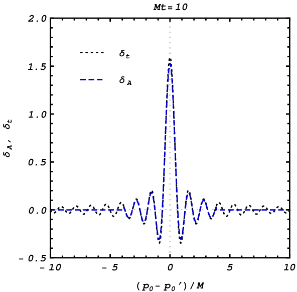
Figure 2: Comparison of $\delta_{t}(p_{0}\>-\>p_{0}^{\prime})$ (black dotted) and $\delta_{A}(p_{0}\>-\>p_{0}^{\prime})$ (blue dashed). The arbitrary mass $M$ is included so that axes are dimensionless.

As we will see later, the oscillatory behavior of the sinc function in $\delta_{t}$ is fundamentally important to the dynamical behavior of the system. Let us therefore convince ourselves that these oscillations persist, even if we smear the switching on of the interactions, or equivalently, if we impose an adiabatic switching off of the interaction Hamiltonian for microscopic times outside the interval $[-\>t/2,\ t/2]$. To this end, we introduce to the interaction Hamiltonian $H^{\rm int}$ in (87) the Gaussian function

$$A_{t}(\tilde{t})\ =\ \exp\!\bigg{(}\!-\frac{\tilde{t}^{2}}{2t^{2}}\bigg{)}\;,$$ (88)

such that the evolution operator takes the form

$$U(\tilde{t}_{f},\tilde{t}_{i})\ =\ \mathrm{T}\exp\bigg{(}\,-i\!\int_{\tilde{t}_{i}}^{\tilde{t}_{f}}\!\!\mathrm{d}{\tilde{t}}\;A_{t}(\tilde{t})H^{\mathrm{int}}(\tilde{t};\tilde{t}_{i})\bigg{)}\;.$$ (89)

Clearly, for $\tilde{t}\>\gg\>t$, $A_{t}(\tilde{t})\>\to\>0$, whereas for $\tilde{t}\>\ll\>t$, $A_{t}(\tilde{t})\>\to\>1$. To account for the effect of $A_{t}(\tilde{t})$ in the action, the following replacement needs to be made:

$$\delta_{t}(p_{0}-p_{0}^{\prime})\ \to\ \delta_{A}(p_{0}\>-\>p_{0}^{\prime})\ \equiv\ \frac{1}{2\pi}\!\int_{-t/2}^{+t/2}\!\mathrm{d}{\tilde{t}}\;e^{-i(p_{0}\>-\>p_{0}^{\prime})\tilde{t}}\,A_{t}(\tilde{t})$$

$$=\ \frac{t}{2\sqrt{2\pi}}\,e^{-\frac{1}{2}(p_{0}\>-\>p_{0}^{\prime})^{2}t^{2}}\bigg{[}\,\mathrm{Erf}\bigg{(}\frac{1\,-\,2i(p_{0}\,-\,p_{0}^{\prime})t}{2\sqrt{2}}\bigg{)}\,+\,\mathrm{Erf}\bigg{(}\frac{1\,+\,2i(p_{0}\,-\,p_{0}^{\prime})t}{2\sqrt{2}}\bigg{)}\bigg{]}\;.$$ (90)

Due to the error functions of complex arguments in (III.3), the oscillatory behavior remains. The analytic behavior of both the functions $\delta_{t}(p_{0}\>-\>p_{0}^{\prime})$ and $\delta_{A}(p_{0}\>-\>p_{0}^{\prime})$ is shown in Figure 2 in which we see that the smooth smearing by the Gaussian function $A_{t}(\tilde{t})$ has little effect on the central region of the sinc function, as one would expect.

IV Non-Homogeneous Backgrounds

Until now, we have considered the vacuum to be an ‘empty’ state with all quantum numbers zero. In this section, we replace that ‘empty’ vacuum state with some macroscopic background, which may in general be inhomogeneous and incoherent. This non-trivial ‘vacuum’ is described by the density operator $\rho$. Following a derivation of the CTP Schwinger–Dyson equation, we show that it is not possible to obtain a closed analytic form for the resummed CTP propagators in the presence of time-dependent backgrounds. Finally, we generalize the discussions in Section III.2 to obtain non-homogeneous free propagators in which space-time translational invariance is explicitly broken.

The density operator $\rho$ is necessarily Hermitian and, for an isolated system, evolves in the interaction picture according to the von Neumann or quantum Liouville equation

$$\frac{\mathrm{d}{\rho(\tilde{t};\tilde{t}_{i})}}{\mathrm{d}{(\tilde{t}-\tilde{t}_{i})}}\ =\ -i\,\big{[}H^{\mathrm{int}}(\tilde{t};\tilde{t}_{i}),\ \rho(\tilde{t};\tilde{t}_{i})\,\big{]}\;,$$ (91)

where $H^{\mathrm{int}}(\tilde{t};\tilde{t}_{i})$ is the interaction part of the Hamiltonian in the interaction picture, which is time-dependent. Notice that the time derivative appearing on the LHS of (91) is taken with respect to the time translationally invariant quantity $\tilde{t}\>-\>\tilde{t}_{i}$. Developing the usual Neumann series, we find that

$$\rho(\tilde{t};\tilde{t}_{i})\ =\ U(\tilde{t},\tilde{t}_{i})\,\rho(\tilde{t}_{i};\tilde{t}_{i})\,U^{-1}(\tilde{t},\tilde{t}_{i})\;,$$ (92)

where $U$ is the evolution operator in (87). Hence, in the absence of external sources and given the unitarity of the evolution operator, the partition function $\mathcal{Z}\>=\>\mathrm{Tr}\,\rho$ is time independent. On the other hand, the partition function of an open or closed subsystem is in general time dependent due to the presence of external sources.

We are interested in evaluating time-dependent Ensemble Expectation Values (EEVs) of field operators $\braket{\bullet}_{t}$ at the macroscopic time $t$, which corresponds to the microscopic time $\tilde{t}_{f}\>=\>t/2$, where the bra-ket now denotes the weighted expectation

$$\braket{\bullet}_{t}\ =\ \frac{\mathrm{Tr}\,\big{(}\,\rho(\tilde{t}_{f};\tilde{t}_{i})\,\bullet\,\big{)}}{\mathrm{Tr}\,\rho(\tilde{t}_{f};\tilde{t}_{i})}\;.$$ (93)

In this case, EEVs of two-point products of field operators begin with a total of nine independent coordinates: the microscopic time of the density operator and the two four-dimensional space-time coordinates of the field operators. As discussed in the beginning of Section III [cf. (33)], this number is reduced to the required seven coordinates, i.e. one temporal and six spatial, after setting all microscopic times equal to $\tilde{t}_{f}\>=\>t/2$. Hence, physical observables in the interaction picture are, for instance, of the form

$$\braket{\Phi(\tilde{t}_{f},\mathbf{x};\tilde{t}_{i})\Phi(\tilde{t}_{f},\mathbf{y};\tilde{t}_{i})}_{t}\ =\ \frac{\mathrm{Tr}\,\big{(}\,\rho(\tilde{t}_{f};\tilde{t}_{i})\Phi(\tilde{t}_{f},\mathbf{x};\tilde{t}_{i})\Phi(\tilde{t}_{f},\mathbf{y};\tilde{t}_{i})\,\big{)}}{\mathrm{Tr}\,\rho(\tilde{t}_{f};\tilde{t}_{i})}\;.$$ (94)

In the presence of a non-trivial background, the out state of Section III is replaced by the density operator $\rho$ at the time of observation $\tilde{t}_{f}\>=\>t/2$. Consequently, the starting point for the CTP generating functional of EEVs is

$$\mathcal{Z}[\rho,J_{\pm},t]\ =\ \mathrm{Tr}\,\Big{[}\Big{(}\bar{\mathrm{T}}e^{-i\!\int_{\Omega_{t}}\!\mathrm{d}^{4}{x}\,J_{-}(x)\Phi_{\mathrm{H}}(x)}\Big{)}\,\rho_{\mathrm{H}}(\tilde{t}_{f};\tilde{t}_{i})\,\Big{(}\mathrm{T}e^{i\!\int_{\Omega_{t}}\!\mathrm{d}^{4}{x}\,J_{+}(x)\Phi_{\mathrm{H}}(x)}\Big{)}\Big{]}\;.$$ (95)

Within the generating functional $\mathcal{Z}$ in (95), the Heisenberg-picture density operator $\rho_{\rm H}$ has explicit time dependence, as it is built out of state vectors that depend on time due to the presence of the external sources $J_{\pm}$. In the absence of such sources, however, the state vectors do not evolve in time, so $\rho_{\rm H}$ and the partition function ${\cal Z}[\rho,J_{\pm}=0,t]\>=\>\mathrm{Tr}\,\rho$ in (95) become time independent quantities.

It is important to emphasize that the explicit microscopic time $\tilde{t}_{f}\>=\>t/2$ of the density operator $\rho_{\mathrm{H}}(\tilde{t}_{f};\tilde{t}_{i})$ appearing in the CTP generating functional (95) is the time of observation. This is in contrast to existing interpretations of the CTP formalism, see for instance Berges (2005), in which the density operator replaces the in state and is therefore fixed at the initial time ${\tilde{t}_{i}\>=\>-t/2}$, encoding only the boundary conditions. As we shall see in Section VIII, this new interpretation of the CTP formalism will lead to the absence of pinch singularities in the resulting perturbation series.

IV.1 The Schwinger–Dyson Equation in the CTP Formalism

In order to generate a perturbation series of correlation functions in the presence of non-homogeneous backgrounds, we must derive the Schwinger–Dyson equation in the CTP formalism. Of particular interest is the explicit form of the Feynman–Dyson series for the expansion of the resummed CTP propagator. We will show that, in the time-dependent case, this series does not collapse to the resummation known from zero-temperature field theory. In particular, we find that a closed analytic form for the resummed CTP propagator is not attainable in general.

We proceed by inserting into the generating functional $\mathcal{Z}$ in (95) complete sets of eigenstates of the Heisenberg field operator $\Phi_{\mathrm{H}}$ at intermediate times via (39). In this way, we obtain the path-integral representation

$$\mathcal{Z}[\rho,J_{a},t]\ =\ \!\int\![\mathrm{d}{\Phi^{a}(\mathbf{x})}]\;\braket{\Phi_{-}(\mathbf{x}),\tilde{t}_{f};\tilde{t}_{i}}{\,\rho_{\mathrm{H}}(\tilde{t}_{f};\tilde{t}_{i})\,}{\Phi_{+}(\mathbf{x}),\tilde{t}_{f};\tilde{t}_{i}}\exp\!\bigg{[}i\bigg{(}\!S[\Phi^{a},t]\>+\>\!\int_{\Omega_{t}}\!\!\mathrm{d}^{4}{x}\;J_{a}(x)\Phi^{a}(x)\bigg{)}\bigg{]}\;.$$ (96)

As before, we may extend the limits of integration to infinity in the free part of the action and the $J$-dependent term, due to the fact that the external sources vanish outside the time interval $[-t/2,\ t/2]$. It is only in the interaction part of the action that the finite domain of integration must remain.

Following Calzetta and Hu (1988), we write the kernel $\braket{\Phi_{-}(\mathbf{x}),\tilde{t}_{f};\tilde{t}_{i}}{\,\rho_{\mathrm{H}}(\tilde{t}_{f};\tilde{t}_{i})\,}{\Phi_{+}(\mathbf{x}),\tilde{t}_{f};\tilde{t}_{i}}$ as an infinite series of poly-local sources:

$$\braket{\Phi_{-}(\mathbf{x}),\tilde{t}_{f};\tilde{t}_{i}}{\,\rho_{\mathrm{H}}(\tilde{t}_{f};\tilde{t}_{i})\,}{\Phi_{+}(\mathbf{x}),\tilde{t}_{f};\tilde{t}_{i}}\ =\ \exp\big{(}iK[\Phi^{a},t\,]\big{)}\;,$$ (97)

where

$$K[\Phi^{a},t\,]\ =\ K\>+\>\!\int_{\Omega_{t}}\!\!\mathrm{d}^{4}{x}\;K_{a}(x,\tilde{t}_{f};\tilde{t}_{i})\Phi^{a}(x)\>+\>\frac{1}{2}\!\iint_{\Omega_{t}}\!\!\mathrm{d}^{4}{x}\,\mathrm{d}^{4}{x^{\prime}}\;K_{ab}(x,x^{\prime},\tilde{t}_{f};\tilde{t}_{i})\Phi^{a}(x)\Phi^{b}(x^{\prime})\>+\>\cdots\;$$ (98)

is a time translationally invariant quantity and only depends on $t\>=\>\tilde{t}_{f}\>-\>\tilde{t}_{i}$. The poly-local sources $K_{ab\cdots}$ encode the state of the system at the microscopic time of observation $\tilde{t}_{f}\>=\>t/2$, i.e. the time at which the EEV is evaluated, according to Figure 1. It follows that these sources must contribute only for $x_{0}\>=\>x_{0}^{\prime}\>=\>\cdots\>=\>\tilde{t}_{f}$ and therefore be proportional to delta functions of the form $\delta(x_{0}\>-\>\tilde{t}_{f})\delta(x_{0}^{\prime}\>-\>\tilde{t}_{f})\cdots$. For instance, the bi-local source $K_{ab}$ in the double momentum representation must have the form

$$K_{ab}(x,x^{\prime},\tilde{t}_{f};\tilde{t}_{i})\ =\ \!\iint\!\!\frac{\mathrm{d}^{4}{p}}{(2\pi)^{4}}\,\frac{\mathrm{d}^{4}{p^{\prime}}}{(2\pi)^{4}}\;e^{-ip\cdot x}\,e^{ip^{\prime}\cdot x^{\prime}}\,e^{i(p_{0}\>-\>p_{0}^{\prime})\tilde{t}_{f}}K_{ab}(\mathbf{p},\mathbf{p}^{\prime},t)\;,$$ (99)

so that the $p_{0}$ and $p_{0}^{\prime}$ integrations yield the required delta functions. Here, it is understood that the bi-local $K_{ab}$ sources occurring on the LHS and RHS of (99) are distinguished by the form of their arguments. We emphasize that $K_{ab}(x,x^{\prime},\tilde{t}_{f};\tilde{t}_{i})$ is not a time translationally invariant quantity due to the explicit dependence upon $\tilde{t}_{f}$ on the RHS of (99). In contrast, $K_{ab}(\mathbf{p},\mathbf{p}^{\prime},t)$ is time translationally invariant.

Notice that we could extend the limits of integration to infinity for the time integrals in the expansion of the kernel given in (98) also. Nevertheless, for the following derivation, all space-time integrals are taken to run over the hypervolume $\Omega_{t}$ in (45) for consistency. We should reiterate here that the limits of time integration can be extended to an infinite domain $\Omega_{\infty}$ in all but the interaction part of the action. We will also suppress the time dependencies of the action $S$ and sources $K_{ab\cdots}$ for notational convenience.

We now absorb the constant $K$ in (98) into the overall normalization of the CTP generating functional ${\cal Z}$ and the local source $K_{a}$ into a redefinition of the external source $J_{a}$. Then, ${\cal Z}$ may be written down as

$$\mathcal{Z}[J_{a},K_{ab},\cdots]\ =\ \!\int\![\mathrm{d}{\Phi^{a}(x)}]\;\exp\!\bigg{[}i\bigg{(}\!S[\Phi^{a}]\>+\>\!\int\!\mathrm{d}^{4}{x}\;J_{a}(x)\Phi^{a}(x)\>+\>\frac{1}{2}\!\iint\!\mathrm{d}^{4}{x}\,\mathrm{d}^{4}{y}\;K_{ab}(x,x^{\prime})\Phi^{a}(x)\Phi^{b}(x^{\prime})$$

$$\qquad+\>\frac{1}{6}\!\iiint\!\mathrm{d}^{4}{x}\,\mathrm{d}^{4}{x^{\prime}}\,\mathrm{d}^{4}{x^{\prime\prime}}\;K_{abc}(x,x^{\prime},x^{\prime\prime})\Phi^{a}(x)\Phi^{b}(x^{\prime})\Phi^{c}(x^{\prime\prime})\>+\>\cdots\bigg{)}\bigg{]}\;.$$ (100)

The Cornwall–Jackiw–Tomboulis (CJT) effective action Cornwall et al. (1974) is given by the following Legendre transform:

$$\Gamma[\widehat{\Phi}^{a},\mathcal{G}^{ab},\mathcal{G}^{abc},\cdots]\ =\ \mathcal{W}[J_{a},K_{ab},K_{abc}]\>-\>\!\int\!\mathrm{d}^{4}{x}\;J_{a}(x)\widehat{\Phi}^{a}(x)$$

$$\qquad-\>\frac{1}{2}\!\iint\!\mathrm{d}^{4}{x}\,\mathrm{d}^{4}{x^{\prime}}\;K_{ab}(x,x^{\prime})\,\Big{(}\,\widehat{\Phi}^{a}(x)\widehat{\Phi}^{b}(x^{\prime})\>+\>i\hbar\mathcal{G}^{ab}(x,x^{\prime})\,\Big{)}$$

$$\qquad-\>\frac{1}{6}\!\iiint\!\mathrm{d}^{4}{x}\,\mathrm{d}^{4}{x^{\prime}}\,\mathrm{d}^{4}{x^{\prime\prime}}\;K_{abc}(x,x^{\prime},x^{\prime\prime})\,\Big{(}\,\widehat{\Phi}^{a}(x)\widehat{\Phi}^{b}(x^{\prime})\widehat{\Phi}^{c}(x^{\prime\prime})$$

$$\qquad+\>3i\hbar\mathcal{G}^{(ab}(x,x^{\prime})\widehat{\Phi}^{c)}(x^{\prime\prime})\>-\>\hbar^{2}\mathcal{G}^{abc}(x,x^{\prime},x^{\prime\prime})\,\Big{)}\>+\>\cdots\;,$$ (101)

where $\mathcal{W}[J_{a},K_{ab},K_{abc},\cdots]\>=\>-i\hbar\ln\mathcal{Z}[J_{a},K_{ab},K_{abc},\cdots]$ is the generating functional of connected ensemble Green’s functions. We obtain an infinite system of equations:

$$\widehat{\Phi}^{a}(x) \ =\ \frac{\delta\mathcal{W}}{\delta J_{a}(x)}\ =\ \braket{\Phi^{a}(x)}\;,$$ (102a)

$$i\hbar\mathcal{G}^{ab}(x,x^{\prime}) \ =\ 2\frac{\delta\mathcal{W}}{\delta K_{ab}(x,x^{\prime})}\>-\>\widehat{\Phi}^{a}(x)\widehat{\Phi}^{b}(x^{\prime})$$

$$\ =\ -i\hbar\frac{\delta^{2}\mathcal{W}}{\delta J_{a}(x)\delta J_{b}(x^{\prime})}\ =\ \braket{\,\mathrm{T}_{\mathcal{C}}\,\big{[}\Phi^{a}(x)\Phi^{b}(x^{\prime})\,\big{]}}\>-\>\braket{\Phi^{a}(x)}\!\braket{\Phi^{b}(x^{\prime})}\;,$$ (102b)

$$-\hbar^{2}\mathcal{G}^{abc}(x,x^{\prime},x^{\prime\prime}) \ =\ 6\frac{\delta\mathcal{W}}{\delta K_{abc}(x,x^{\prime},x^{\prime\prime})}\>-\>3i\hbar\mathcal{G}^{(ab}(x,x^{\prime})\widehat{\Phi}^{c)}(x^{\prime\prime})\>-\>\widehat{\Phi}^{a}(x)\widehat{\Phi}^{b}(x^{\prime})\widehat{\Phi}^{c}(x^{\prime\prime})$$

$$\ =\ -\hbar^{2}\frac{\delta^{3}\mathcal{W}}{\delta J_{a}(x)\delta J_{b}(x^{\prime})\delta J_{c}(x^{\prime\prime})}\;,$$ (102c)

and

$$\frac{\delta\Gamma}{\delta\widehat{\Phi}^{a}(x)}\ =\ -J_{a}(x)\>-\>\int\!\mathrm{d}^{4}{x^{\prime}}\;K_{ab}(x,x^{\prime})\widehat{\Phi}^{b}(x^{\prime})$$

$$\qquad-\>\frac{1}{2}\!\iint\!\mathrm{d}^{4}{x^{\prime}}\,\mathrm{d}^{4}{x^{\prime\prime}}\;K_{abc}(x,x^{\prime},x^{\prime\prime})\,\Big{(}\,\widehat{\Phi}^{b}(x^{\prime})\widehat{\Phi}^{c}(x^{\prime\prime})\>+\>i\hbar\mathcal{G}^{bc}(x^{\prime},x^{\prime\prime})\,\Big{)}\>-\>\cdots\;,$$ (103a)

$$\frac{\delta\Gamma}{\delta\mathcal{G}^{ab}(x,x^{\prime})}\ =\ -\frac{i\hbar}{2}K_{ab}(x,x^{\prime})\>-\>\frac{i\hbar}{2}\!\int\!\mathrm{d}^{4}{x^{\prime\prime}}\;K_{abc}(x,x^{\prime},x^{\prime\prime})\widehat{\Phi}^{c}(x^{\prime\prime})\>-\>\cdots\;,$$ (103b)

$$\frac{\delta\Gamma}{\delta\mathcal{G}^{abc}(x,x^{\prime},x^{\prime\prime})}\ =\ \frac{\hbar^{2}}{6}K_{abc}(x,x^{\prime},x^{\prime\prime})\>+\>\cdots\;,$$ (103c)

where the parentheses $(abc)$ on the RHS of (102) denote cyclic permutation with respect to the indices $a$, $b$, $c$.

The above infinite system of equations (102) and (103) may be simplified by assuming that the density operator $\rho$ is Gaussian, as we will do later in Section IV.3. In this case, the tri-local and higher kernels ($K_{abc}$, $K_{abcd}$, $\cdots$) can be set to zero in (103), neglecting contributions from thermally-corrected vertices [see (IV.3)], which would otherwise be present for non-Gaussian density operators. Within the Gaussian approximation, the three- and higher-point connected Green’s functions ($\mathcal{G}^{abc}$, $\mathcal{G}^{abcd}$, $\cdots$) may be eliminated as dynamical variables by performing a second Legendre transform

$$\Gamma[\widehat{\Phi}^{a},\mathcal{G}^{ab}]\ \equiv\ \Gamma[\widehat{\Phi}^{a},\mathcal{G}^{ab},\widetilde{\mathcal{G}}^{abc},\cdots]\;,$$ (104)

where the $\widetilde{\mathcal{G}}$’s are functionals of $\widehat{\Phi}^{a}$ and $\mathcal{G}^{ab}$ given by

$$\frac{\delta\Gamma}{\delta\mathcal{G}^{abc\cdots}}[\widehat{\Phi}^{a},\mathcal{G}^{ab},\widetilde{\mathcal{G}}^{abc},\cdots]\ =\ 0\;.$$ (105)

The effective action is evaluated by expanding around the constant background field $\Phi_{0}^{a}(x)\ =\ \Phi^{a}(x)\>-\>\hbar^{1/2}\phi^{a}(x)$, defined at the saddle point

$$\frac{\delta S[\Phi^{a}]}{\delta\Phi^{a}(x)}\Bigg{|}_{\Phi\>=\>\Phi_{0}}\>+\>J_{a}(x)\>+\>\!\int\!\mathrm{d}^{4}{x^{\prime}}\;K_{ab}(x,x^{\prime})\Phi_{0}^{b}(x^{\prime})\ =\ 0\;.$$ (106)

The result of this expansion is well known Cornwall et al. (1974); Carrington (2004) and, truncating to order $\hbar^{2}$, we obtain the two-particle-irreducible (2PI) CJT effective action

$$\Gamma[\widehat{\Phi}^{a},\mathcal{G}^{ab}]\ =\ S[\widehat{\Phi}^{a}]\>+\>\frac{i\hbar}{2}\,\mathrm{Tr}_{x}\Big{[}\,\mathrm{Ln}_{x}\,\mathrm{Det}_{ab}\,\mathcal{G}_{ab}^{-1}\>+\>\Big{(}\,G_{ab}^{-1}\>-\>K_{ab}\,\Big{)}*\mathcal{G}^{ab}\>-\>\eta_{a}^{\;a}\,\Big{]}\>+\>\hbar^{2}\Gamma_{2}[\widehat{\Phi}^{a},\mathcal{G}^{ab}]\;,$$ (107)

where a subscript $x$ and the $*$’s indicate that the trace, logarithm and products should be understood as functional operations. The operator $G^{-1}_{ab}$ is defined by

$$G_{ab}^{-1}(\widehat{\Phi}^{a};x,x^{\prime})\ =\ \frac{\delta^{2}S[\widehat{\Phi}^{a}]}{\delta\widehat{\Phi}^{a}(x)\delta\widehat{\Phi}^{b}(x^{\prime})}\>+\>K_{ab}(x,x^{\prime})\ =\ \Delta_{ab}^{0,\,-1}(x,x^{\prime})\>+\>\frac{\delta^{2}S^{\mathrm{int}}[\widehat{\Phi}^{a}]}{\delta\widehat{\Phi}^{a}(x)\delta\widehat{\Phi}^{b}(x^{\prime})}\>+\>K_{ab}(x,x^{\prime})\;,$$ (108)

where $\Delta_{ab}^{0,\,-1}(x,x^{\prime})$ is the free inverse CTP propagator in (55) and $S^{\mathrm{int}}[\widehat{\Phi}^{a}]$ is the interaction part of the action. Obviously, all Green’s functions depend upon the state of the system at the macroscopic time $t$ through the bi-local source $K_{ab}$. For the Lagrangian in (1), we have

$$G_{ab}^{-1}(\widehat{\Phi}^{a};x,x^{\prime})\ =\ \delta^{(4)}(x\>-\>x^{\prime})\Big{[}\,-\big{(}\Box^{2}_{x}\>+\>M^{2}\big{)}\eta_{ab}\>+\>i\epsilon\mathbb{I}_{ab}\>-\>g\eta_{abc}\widehat{\Phi}^{c}(x)\>-\>\frac{1}{2}\lambda\eta_{abcd}\widehat{\Phi}^{c}(x)\widehat{\Phi}^{d}(x)\Big{]}\>+\>K_{ab}(x,x^{\prime})\;,$$ (109)

where $\eta_{abc\cdots}\>=\>+1$ for all indices $a\>=\>b\>=\>\cdots\>=\>1$, $\eta_{abc\cdots}\>=\>-1$ for all indices $a\>=\>b\>=\>\cdots\>=\>2$ and $\eta_{abc\cdots}\>=\>0$ otherwise.

The overall normalization ($\eta_{a}^{\;a}$) of (107) has been chosen so that when ${K_{ab}(x,x^{\prime})\>=\>0}$, we may recover the conventional effective action Jackiw (1974) by making a further Legendre transform to eliminate $\mathcal{G}^{ab}$ as a dynamical variable:

$$\Gamma[\widehat{\Phi}^{a}]\ \equiv\ \Gamma[\widehat{\Phi}^{a},\widetilde{\mathcal{G}}^{ab}]\ =\ S[\widehat{\Phi}^{a}]\>+\>\frac{i\hbar}{2}\mathrm{Tr}_{x}\,\mathrm{Ln}_{x}\,\mathrm{Det}_{ab}\,G_{ab}^{-1}\>+\>\mathcal{O}(\hbar^{2})\;.$$ (110)

Here, $\mathcal{G}^{-1}_{ab}$ has been replaced by $G^{-1}_{ab}$ and $\widetilde{\mathcal{G}}^{ab}$ is a functional of $\widehat{\Phi}^{a}$.

In the CJT effective action (107), $\Gamma_{2}[\widehat{\Phi}^{a},\mathcal{G}^{ab}]$ is the sum of all 2PI vacuum graphs:

$$\Gamma_{2}[\widehat{\Phi}^{a},\mathcal{G}^{ab}]\ =\ -i\sum_{a,\,b\>=\>1,\,2}\Bigg{[}\frac{1}{8}\,\parbox[0.0pt][c]{62.59596pt}{ \includegraphics{2bubble.pdf}}\delta_{ab}\,\>+\>\frac{1}{12}\parbox[0.0pt][c]{54.06006pt}{\includegraphics{sunset.pdf}}\,\Bigg{]}\;,\vspace{-1em}$$ (111)

where combinatorial factors have been written explicitly and we associate with each $n$-point vertex a factor of

$$iS^{(n)}_{a}(\widehat{\Phi}^{a};x)\ =\ i\frac{\delta^{n}S[\widehat{\Phi}^{a}]}{\delta\big{(}\widehat{\Phi}^{a}(x)\big{)}^{n}}\;,$$ (112)

and each line a factor of $i\mathcal{G}^{ab}(\widehat{\Phi}^{a};x,y)$. The three- and four-point vertices are

$$iS_{a}^{(3)}(\widehat{\Phi}^{a};x)\ =\ -ig\eta_{aaa}\>-\>i\lambda\eta_{aaaa}\widehat{\Phi}^{a}(x)\;,\qquad iS_{a}^{(4)}(\widehat{\Phi}^{a};x)\ =\ -i\lambda\eta_{aaaa}\;.$$ (113)

Upon functional differentiation of the CJT effective action (107) with respect to $\mathcal{G}^{ab}(x,y)$, we obtain by virtue of (103b) the Schwinger–Dyson equation

$$\mathcal{G}^{-1}_{ab}(\widehat{\Phi}^{a};x,y)\ =\ G_{ab}^{-1}(\widehat{\Phi}^{a};x,y)\>+\>\Pi_{ab}(\widehat{\Phi}^{a},\mathcal{G}^{ab};x,y)\;,$$ (114)

where

$$\Pi_{ab}(\widehat{\Phi}^{a},\mathcal{G}^{ab};x,y)\ =\ -2i\hbar\frac{\delta\Gamma_{2}[\widehat{\Phi}^{a},\mathcal{G}^{ab}]}{\delta\mathcal{G}^{ab}(x,y)}\ =\ -i\hbar\Bigg{[}\>\parbox[0.0pt][t]{91.04872pt}{ \includegraphics{self1.pdf}}\delta_{ab}\>+\>\,\parbox[0.0pt][c]{91.04872pt}{\includegraphics{self2.pdf}}\Bigg{]}$$ (115)

is the one-loop truncated CTP self-energy. A combinatorial factor of $\frac{1}{2}$ has been absorbed into the diagrammatics.

Suppressing the $\widehat{\Phi}^{a}$ and $\mathcal{G}^{ab}$ arguments for notational convenience, the CTP self-energy $\Pi_{ab}(x,y)$ may be written in matrix form as

$$\Pi_{ab}(x,y)\ =\ \begin{bmatrix}\Pi(x,y)&-\Pi_{<}(x,y)\\ -\Pi_{>}(x,y)&-\Pi^{*}(x,y)\end{bmatrix}\!\;,$$ (116)

where $\Pi(x,y)$ and $-\Pi^{*}(x,y)$ are the time- and anti-time-ordered self-energies; and $\Pi_{>}(x,y)$ and $\Pi_{<}(x,y)$ are the positive- and negative-frequency absolutely-ordered self-energies, respectively. In analogy to the propagator definitions discussed in Section II and Appendix A, we also define the self-energy functions

$$\Pi_{1}(x,y) \ =\ \Pi_{>}(x,y)\>+\>\Pi_{<}(x,y)\ =\ \Pi(x,y)\>-\>\Pi^{*}(x,y)\ =\ 2i\,\mathrm{Im}\,\Pi(x,y)\;,$$ (117a)

$$\Pi_{\mathcal{P}}(x,y) \ =\ \frac{1}{2}\Big{(}\,\Pi_{\mathrm{R}}(x,y)\>+\>\Pi_{\mathrm{A}}(x,y)\,\Big{)}\ =\ \mathrm{Re}\,\Pi(x,y)\;,$$ (117b)

$$2iM\Gamma(x,y) \ =\ \Pi_{>}(x,y)\>-\>\Pi_{<}(x,y)\ =\ \Pi_{\mathrm{R}}(x,y)\>-\>\Pi_{\mathrm{A}}(x,y)\ =\ 2i\,\mathrm{Im}\,\Pi_{\mathrm{R}}(x,y)\;,$$ (117c)

which satisfy relations analogous to those described in Appendix A. $\Gamma(x,y)$ in (117c) is related to the usual Breit–Wigner width in the equilibrium and zero-temperature limits. The Keldysh representation [see (52)] $\widetilde{\Pi}_{ab}(x,y)$ of the CTP self-energy reads:

$$\widetilde{\Pi}_{ab}(x,y)\ =\ \begin{bmatrix}\Pi_{1}(x,y)&\Pi_{\mathrm{R}}(x,y)\\ \Pi_{\mathrm{A}}(x,y)&0\end{bmatrix}\!\;.$$ (118)

In the limit $\widehat{\Phi}^{a}(x)\>\to\>0$, the Schwinger–Dyson equation (114) reduces to

$$\Delta^{-1}_{ab}(x,y,\tilde{t}_{f};\tilde{t}_{i})\ =\ \Delta_{ab}^{0,\,-1}(x,y)\>+\>K_{ab}(x,y,\tilde{t}_{f};\tilde{t}_{i})\>+\>\Pi_{ab}(x,y,\tilde{t}_{f};\tilde{t}_{i})\;,$$ (119)

in which $\Delta^{-1}_{ab}(x,y,\tilde{t}_{f};\tilde{t}_{i})\>\equiv\>\mathcal{G}_{ab}^{-1}(\widehat{\Phi}^{a}=0;x,y,\tilde{t}_{f};\tilde{t}_{i})$ and $\Delta_{ab}^{0,\,-1}(x,y)$ is the free inverse CTP propagator defined in (55). We have re-introduced the dependence upon $\tilde{t}_{f}$ and $\tilde{t}_{i}$ for clarity. Notice that due to the explicit $\tilde{t}_{f}$ dependence of the bi-local source $K_{ab}(x,y,\tilde{t}_{f};\tilde{t}_{i})$ in (99), the inverse resummed CTP propagator ${\Delta^{-1}_{ab}(x,y,\tilde{t}_{f};\tilde{t}_{i})}$ and the CTP self-energy ${\Pi_{ab}(x,y,\tilde{t}_{f};\tilde{t}_{i})}$ are not time translationally invariant quantities.

In order to develop a self-consistent inversion of the Schwinger–Dyson equation in (119), the bi-local source $K_{ab}(x,y,\tilde{t}_{f};\tilde{t}_{i})$ is absorbed into an inverse non-homogeneous CTP propagator

$$D^{0,\,-1}_{ab}(x,y,\tilde{t}_{f};\tilde{t}_{i})\ =\ \Delta_{ab}^{0,\,-1}(x,y)\>+\>K_{ab}(x,y,\tilde{t}_{f};\tilde{t}_{i}),$$ (120)

whose inverse, to leading order in $K_{ab}$, is the free CTP propagator $\Delta^{0,\,ab}(x,y,\tilde{t}_{f};\tilde{t}_{i})$, i.e.

$$D^{0,\,ab}(x,y,\tilde{t}_{f};\tilde{t}_{i})\ \equiv\ \Delta^{0,\,ab}(x,y,\tilde{t}_{f};\tilde{t}_{i})\>+\>\mathcal{O}(K^{2})\;,$$ (121)

as we will illustrate in Sections IV.3 and V. The contribution of the bi-local source $K_{ab}$ is now absorbed into the free CTP propagator $\Delta^{0,\,ab}(x,y,\tilde{t}_{f};\tilde{t}_{i})$, whose time translational invariance is broken as a result. The Schwinger–Dyson equation (119) may then be written in the double momentum representation as

$$\Delta^{-1}_{ab}(p,p^{\prime},\tilde{t}_{f};\tilde{t}_{i})\ =\ \Delta_{ab}^{0,\,-1}(p,p^{\prime})\>+\>\Pi_{ab}(p,p^{\prime},\tilde{t}_{f};\tilde{t}_{i})\;.$$ (122)

Since the stationary vacuum $\ket{0}$ has been replaced by the density operator $\rho$ at the microscopic time $\tilde{t}_{f}\>=\>t/2$, we must consider the following field-particle duality relation in the Wick contraction of interaction-picture fields:

$$\braket{0}{\Phi(x;\tilde{t}_{i})a^{{\dagger}}(\mathbf{k},\tilde{t}_{f};\tilde{t}_{i})}{0} \ =\ e^{-ik\cdot x}e^{iE(\mathbf{k})\tilde{t}_{f}}\;.$$ (123)

Here, the extra phase $e^{iE(\mathbf{k})\tilde{t}_{f}}$ arises from the fact that the creation and annihilation operators of the interaction-picture field $\Phi(x;\tilde{t}_{i})$ are evaluated at the microscopic time $\tilde{t}\>=\>0$ [cf. (12) and (18)], whereas the operator $a^{{\dagger}}(\mathbf{k},\tilde{t}_{f};\tilde{t}_{i})$, resulting from the expansion of the density operator $\rho$ (see Section IV.3), is evaluated at the microscopic time $\tilde{t}_{f}\>=\>t/2$. Analytically continuing this extra phase to off-shell energies and in consistency with (99), we associate with each external vertex of the self-energy $\Pi_{ab}(p,p^{\prime},\tilde{t}_{f};\tilde{t}_{i})$ in (122) a phase:

$$e^{ip_{0}\tilde{t}_{f}}\,,$$ (124)

where $p_{0}$ is the energy flowing into the vertex. This amounts to the absorption of an overall phase

$$e^{i(p_{0}\>-\>p_{0}^{\prime})\tilde{t}_{f}}$$ (125)

into the definition of the self-energy $\Pi_{ab}(p,p^{\prime},\tilde{t}_{f};\tilde{t}_{i})$.

Convoluting from left and right on both sides of (122) first with the weight function $(2\pi)^{4}\delta_{t}^{(4)}(p\>-\>p^{\prime})$ from (84) and then with $\Delta^{0,\,ab}(p,p^{\prime},\tilde{t}_{f};\tilde{t}_{i})$ and $\Delta^{ab}(p,p^{\prime},\tilde{t}_{f};\tilde{t}_{i})$, respectively, we obtain the Feynman–Dyson series

$$\Delta^{ab}(p,p^{\prime},\tilde{t}_{f};\tilde{t}_{i})\ =\ \Delta^{0,\,ab}(p,p^{\prime},\tilde{t}_{f};\tilde{t}_{i})\>-\>\!\idotsint\!\!\frac{\mathrm{d}^{4}{q}}{(2\pi)^{4}}\,\frac{\mathrm{d}^{4}{q^{\prime}}}{(2\pi)^{4}}\,\frac{\mathrm{d}^{4}{q^{\prime\prime}}}{(2\pi)^{4}}\,\frac{\mathrm{d}^{4}{q^{\prime\prime\prime}}}{(2\pi)^{4}}$$

$$\qquad\times\>\Delta^{0,\,ac}(p,q,\tilde{t}_{f};\tilde{t}_{i})(2\pi)^{4}\delta_{t}^{(4)}(q\>-\>q^{\prime})\Pi_{cd}(q^{\prime},q^{\prime\prime},\tilde{t}_{f};\tilde{t}_{i})(2\pi)^{4}\delta_{t}^{(4)}(q^{\prime\prime}\>-\>q^{\prime\prime\prime})\Delta^{db}(q^{\prime\prime\prime},p^{\prime},\tilde{t}_{f};\tilde{t}_{i})\;,$$ (126)

where $\delta_{t}^{(4)}(p\>-\>p^{\prime})$ is defined in (83). Because of the form of $\delta_{t}(p_{0}\>-\>p_{0}^{\prime})$ in (84), we see that this series does not collapse to an algebraic equation of resummation, as known from zero-temperature field theory. As we will see in Section IV.2, one cannot write down a closed analytic form for the resummed CTP propagator $\Delta^{ab}(p,p^{\prime},\tilde{t}_{f};\tilde{t}_{i})$, except in the thermodynamic equilibrium limit, see Section V.

Given that $\delta_{t}$ satisfies the convolution in (86), the weight functions may be absorbed into the external vertices of the self-energy $\Pi_{ab}(p,p^{\prime},\tilde{t}_{f};\tilde{t}_{i})$; see Section IX. The Feynman–Dyson series may then be written in the more concise form

$$\Delta^{ab}(p,p^{\prime},\tilde{t}_{f};\tilde{t}_{i})\ =\ \Delta^{0,\,ab}(p,p^{\prime},\tilde{t}_{f};\tilde{t}_{i})\>-\>\!\iint\!\!\frac{\mathrm{d}^{4}{q}}{(2\pi)^{4}}\,\frac{\mathrm{d}^{4}{q^{\prime}}}{(2\pi)^{4}}\;\Delta^{0,\,ac}(p,q,\tilde{t}_{f};\tilde{t}_{i})\Pi_{cd}(q,q^{\prime},\tilde{t}_{f};\tilde{t}_{i})\Delta^{db}(q^{\prime},p^{\prime},\tilde{t}_{f};\tilde{t}_{i})\;.$$ (127)

Note that for finite $t$, $\delta_{t}(p_{0}\>-\>p_{0}^{\prime})$ is analytic for all $p_{0}$, including $p_{0}\>=\>p_{0}^{\prime}$. As we shall see in Section VIII, the systematic incorporation of these finite-time effects ensures that the perturbation expansion is free of pinch singularities.

IV.2 Applicability of the Gradient Expansion

Here, we will look more closely at the inverse relation (81) that determines the resummed CTP propagator. We will show that a full matrix inversion may only be performed in the thermodynamic equilibrium limit. Hence, the application of truncated gradient expansions and the use of partially resummed quasi-particle propagators, particularly for early times, become questionable in out-of-equilibrium systems.

We define the relative and central coordinates

$$R_{xy}^{\mu}\ =\ x^{\mu}\>-\>y^{\mu}\;,\qquad X_{xy}^{\mu}\ =\ \frac{x^{\mu}\>+\>y^{\mu}}{2}\;,$$ (128)

such that

$$x^{\mu}\ =\ X_{xy}^{\mu}\>+\>\frac{1}{2}R_{xy}^{\mu}\;,\qquad y^{\mu}\ =\ X^{\mu}_{xy}\>-\>\frac{1}{2}R_{xy}^{\mu}\;.$$ (129)

We then introduce the Wigner transform (see Winter (1985)), namely the Fourier transform with respect to the relative coordinate $R^{\mu}_{xy}$ only. Explicitly, the Wigner transform of a function $F(R,X)$ is

$$F(p,X)\ =\ \!\int\!\mathrm{d}^{4}{R}\;e^{ip\cdot R}\,F(R,X)\;.$$ (130)

The resummed CTP propagator $\Delta^{ab}(x,y)$ respects the inverse relation in (81). Here, we suppress the $\tilde{t}_{f}$ and $\tilde{t}_{i}$ dependence of the propagators for notational convenience. Inserting into (81), the Wigner transforms of the resummed and inverse resummed CTP propagators, the inverse relation takes the form

$$\int_{\Omega_{t}}\!\mathrm{d}^{4}{z}\iint\!\!\frac{\mathrm{d}^{4}{p}}{(2\pi)^{4}}\,\frac{\mathrm{d}^{4}{p^{\prime}}}{(2\pi)^{4}}\,e^{-ip\cdot R_{xz}}\,e^{-ip^{\prime}\cdot R_{zy}}\,\Delta_{ab}^{-1}(p,X_{xz})\Delta^{bc}(p^{\prime},X_{zy})\ =\ \iint\!\!\frac{\mathrm{d}^{4}{p}}{(2\pi)^{4}}\,\frac{\mathrm{d}^{4}{p^{\prime}}}{(2\pi)^{4}}\,e^{-ip\cdot x}\,e^{ip^{\prime}\cdot y}\,\eta_{a}^{\;c}(2\pi)^{4}\delta^{(4)}_{t}(p\>-\>p^{\prime})\;,$$ (131)

where the $z^{0}$ domain of integration is restricted to be in the range $[-t/2,\ t/2]$.

In the case where deviations from homogeneity are small, i.e. when the characteristic scale of macroscopic variations in the background is large in comparison to that of the microscopic single-particle excitations, we may perform a gradient expansion of the inverse relation in terms of the soft derivative $\partial_{X_{xy}}^{\mu}\>\equiv\>\partial/\partial X_{xy,\,\mu}$. Writing $X_{xz}\>=\>X_{xy}\>+\>R_{zy}/2$ and $X_{zy}\>=\>X_{xy}\>-\>R_{xz}/2$ and after integrating by parts, we obtain

$$\iint\!\!\frac{\mathrm{d}^{4}{p}}{(2\pi)^{4}}\,\frac{\mathrm{d}^{4}{p^{\prime}}}{(2\pi)^{4}}\,e^{-ip\cdot x}\,e^{ip^{\prime}\cdot y}\,(2\pi)^{4}\delta_{t}^{(4)}(p-p^{\prime})\Big{\{}\Delta_{ab}^{-1}(p,X)\exp\!\Big{[}-\frac{i}{2}\big{(}\overleftarrow{\partial_{p}}\cdot\overrightarrow{\partial_{X}}\>-\>\overleftarrow{\partial_{X}}\cdot\overrightarrow{\partial_{p^{\prime}}}\big{)}\Big{]}\Delta^{bc}(p^{\prime},X)\Big{\}}$$

$$\qquad\qquad=\ \!\iint\!\!\frac{\mathrm{d}^{4}{p}}{(2\pi)^{4}}\,\frac{\mathrm{d}^{4}{p^{\prime}}}{(2\pi)^{4}}\,e^{-ip\cdot x}\,e^{ip^{\prime}\cdot y}\,\eta_{a}^{\;c}(2\pi)^{4}\delta^{(4)}_{t}(p\>-\>p^{\prime})\;,$$ (132)

where $X\>\equiv\>X_{xy}$ and the derivatives act only within the curly brackets.

We now define the central and relative momenta

$$q^{\mu}\ =\ \frac{p^{\mu}\>+\>p^{\prime\mu}}{2}\;,\qquad Q^{\mu}\ =\ p^{\mu}\>-\>p^{\prime\mu}\;,$$ (133)

which are the Fourier conjugates to the relative and central coordinates, $R^{\mu}$ and $X^{\mu}$, respectively. It follows that

$$p^{\mu}\ =\ q^{\mu}\>+\>\frac{1}{2}Q^{\mu}\;,\qquad p^{\prime\mu}\ =\ q^{\mu}\>-\>\frac{1}{2}Q^{\mu}\;.$$ (134)

We may then Fourier transform (IV.2) with respect to $R_{xy}$ to obtain

$$\int\!\!\frac{\mathrm{d}^{4}{Q}}{(2\pi)^{4}}\;e^{-iQ\cdot X}\,(2\pi)^{4}\delta_{t}^{(4)}(Q)\exp\!\Big{[}\,-i\,\Big{(}\,\diamondsuit_{q,X}^{-}\>+\>2\diamondsuit^{+}_{Q,X}\,\Big{)}\Big{]}\{\Delta_{ab}^{-1}(q+\tfrac{Q}{2},X)\}\{\Delta^{bc}(q-\tfrac{Q}{2},X)\}$$

$$\qquad\qquad=\ \int\!\!\frac{\mathrm{d}^{4}{Q}}{(2\pi)^{4}}\,e^{-iQ\cdot X}\,\eta_{a}^{\;c}(2\pi)^{4}\delta_{t}^{(4)}(Q)\;,$$ (135)

where, following Cassing and Juchem (2000); Prokopec et al. (2004a, b), we have introduced the diamond operator

$$\diamondsuit_{p,X}^{\pm}\{A\}\{B\}\ =\ \frac{1}{2}\{A,\ B\}^{\pm}_{p,X}$$ (136)

and $\{A,\ B\}^{\pm}_{p,X}$ denote the symmetric and anti-symmetric Poisson brackets

$$\{A,\ B\}^{\pm}_{p,X}\ \equiv\ \frac{\partial A}{\partial p^{\mu}}\,\frac{\partial B}{\partial X_{\mu}}\>\pm\>\frac{\partial A}{\partial X^{\mu}}\,\frac{\partial B}{\partial p_{\mu}}\;.$$ (137)

For $t>0$, we may perform the integral on the RHS of (IV.2), yielding

$$\int\!\!\frac{\mathrm{d}^{4}{Q}}{(2\pi)^{4}}\;e^{-iQ\cdot X}\,(2\pi)^{4}\delta_{t}^{(4)}(Q)\exp\!\Big{[}-i\,\Big{(}\,\diamondsuit_{q,X}^{-}\>+\>2\diamondsuit^{+}_{Q,X}\,\Big{)}\Big{]}\{\Delta_{ab}^{-1}(q+\tfrac{Q}{2},X)\}\{\Delta^{bc}(q-\tfrac{Q}{2},X)\}\ =\ \eta_{a}^{\;c}\theta(t-2|X_{0}|)\;,$$ (138)

In the above expressions, of particular concern is the $\diamondsuit^{+}_{Q,X}$ operator, where the relative momentum $Q$ and the central coordinate $X$ are conjugate to one another. Thus, if the derivatives with respect to $X$ are assumed to be small, then the derivatives with respect to $Q$ must be large. In this case, all orders of the gradient expansion may be significant, so it is inappropriate to truncate to a given order in the soft derivative $\partial_{X}^{\mu}$.

As $t\>\to\>\infty$, we have the transition $\delta^{(4)}_{t}(Q)\>\to\>\delta^{(4)}(Q)$ and (138) reduces to

$$e^{-i\diamondsuit^{-}_{q,X}}\{\Delta^{-1}_{ab}(q,X)\}\{\Delta^{bc}(q,X)\}\ =\ \eta_{a}^{\;c}\;.$$ (139)

Even for these late times, we can perform the matrix inversion exactly only if we truncate the gradient expansion in (139) to zeroth order. However, such a truncation appears valid only for time-independent and spatially homogeneous systems. Employing a suitable quasi-particle approximation to the Wigner representation of the propagators, it can be shown Bornath et al. (1996) that this inversion may be performed at first order in the gradient expansion. However, off-shell contributions are not fully accounted for in such an approximation.

In conclusion, a closed analytic form for the resummed CTP propagator may only be obtained in the time-independent thermodynamic equilibrium limit. The truncation of the gradient expansion may be justifiable only to the late-time evolution of systems very close to equilibrium, even for spatially homogeneous thermal backgrounds. A similar conclusion is drawn from different arguments in Berges and Borsányi (2006).

IV.3 Non-Homogeneous Free Propagators

Unlike the resummed CTP propagator, the free CTP propagator can be derived analytically, even in the presence of a time-dependent and spatially inhomogeneous background. The non-homogeneous free propagator will account explicitly for the violation of space-time translational invariance. Our derivation relies on the algebra of the canonical quantization commutators of creation and annihilation operators described in Section II. Subsequently, we make connection of our results with the path-integral representation of the CTP generating functional in (IV.1). Finally, we introduce a diagrammatic representation for the non-homogeneous free CTP propagator.

We note that the derived propagators are ‘free’ in the sense that their spectral structure is that of single-particle states, corresponding to the free part of the action (see Section III). Their statistical structure, on the other hand, will turn out to contain a summation over contributions from all possible multi-particle states. The time-dependent statistical distribution function appearing in these propagators is therefore a statistically-dressed object. This subtle point is significant for the consistent definition of the number density in Section VI, the derivation of the master time evolution equations in Section VII and the absence of pinch singularities, described in Section VIII.

The starting point of our canonical derivation is the explicit form of the density operator $\rho$. We relax any assumptions about the form of the density operator and take it to be in general non-diagonal but Hermitian within the general Fock space. We may write the most general interaction-picture density operator at the microscopic time $\tilde{t}_{f}\>=\>t/2$ as

$$\rho(\tilde{t}_{f};\tilde{t}_{i})\ =\ C\exp\!\bigg{[}-\!\int\!\mathrm{d}{\Pi_{\mathbf{k}_{1}}}\;W_{10}(\mathbf{k}_{1}:0)a^{{\dagger}}(\mathbf{k}_{1},\tilde{t}_{f})\>-\>\!\int\!\mathrm{d}{\Pi_{\mathbf{k}_{1}^{\prime}}}\;W_{01}(0:\mathbf{k}_{1}^{\prime})a(\mathbf{k}_{1}^{\prime},\tilde{t}_{f})$$

$$\qquad-\>\!\iint\!\mathrm{d}{\Pi_{\mathbf{k}_{1}}}\,\mathrm{d}{\Pi_{\mathbf{k}_{1}^{\prime}}}\;W_{11}(\mathbf{k}_{1}:\mathbf{k}_{1}^{\prime})a^{{\dagger}}(\mathbf{k}_{1},\tilde{t}_{f})a(\mathbf{k}_{1}^{\prime},\tilde{t}_{f})\>-\>\cdots$$

$$\qquad-\>\!\frac{1}{n!}\frac{1}{m!}\!\idotsint\!\Bigg{(}\prod_{i=1}^{n}\mathrm{d}{\Pi_{\mathbf{k}_{i}}}\bigg{)}\bigg{(}\prod_{j=1}^{m}\mathrm{d}{\Pi_{\mathbf{k}_{j}^{\prime}}}\bigg{)}\;W_{nm}(\{\mathbf{k}_{i}\}:\{\mathbf{k}_{j}^{\prime}\})\prod_{i=1}^{n}a^{{\dagger}}(\mathbf{k}_{i},\tilde{t}_{f})\prod_{j=1}^{m}a(\mathbf{k}_{j}^{\prime},\tilde{t}_{f})\bigg{]}\;,$$ (140)

where the constant $C$ can be set to unity without loss of generality. The complex-valued weights $W_{nm}(\{\mathbf{k}\}_{n};\{\mathbf{k}^{\prime}\}_{m})$ depend on the state of the system at time $\tilde{t}_{f}\>=\>t/2$ and satisfy the Hermiticity constraint:

$$W_{nm}(\{\mathbf{k}\}_{n}:\{\mathbf{k}^{\prime}\}_{m})\ =\ W_{mn}^{*}(\{\mathbf{k}^{\prime}\}_{m}:\{\mathbf{k}\}_{n})\;.$$ (141)

The density operator $\rho$ may be written in the basis of momentum eigenstates by multiplying the exponential form in (IV.3) by the completeness relation of the basis of Fock states at time $\tilde{t}_{f}\>=\>t/2$:

$$\mathbf{I}\ =\ \ket{0}\!\bra{0}\>+\>\sum_{\ell\>=\>1}^{\infty}\frac{1}{\ell!}\bigg{(}\prod_{k=1}^{\ell}\int\!\mathrm{d}{\Pi_{\mathbf{p}_{k}}}\bigg{)}\!\ket{\{\mathbf{p}\}_{\ell},\tilde{t}_{f}}\!\bra{\{\mathbf{p}\}_{\ell},\tilde{t}_{f}}\;,$$ (142)

where $\ket{\{\mathbf{p}\}_{\ell},\tilde{t}_{f}}$ is the multi-mode Fock state $\ket{\mathbf{p}_{1},\tilde{t}_{f}}\>\otimes\>\ket{\mathbf{p}_{2},\tilde{t}_{f}}\>\otimes\>\cdots\>\otimes\>\ket{\mathbf{p}_{\ell},\tilde{t}_{f}}$. This usually gives an intractable infinite series of $n$-to-$m$-particle correlations. Taking all weights $W_{nm}(\{\mathbf{k}\}_{n}:\{\mathbf{k}\}_{m})$ to be zero if $n\>+\>m\>>\>2$, i.e. taking a Gaussian-like density operator, it is still possible to generate all possible $n$-to-$m$-particle correlations. In Appendix D, we give the expansion of the general Gaussian-like density operator, where only sufficient terms are included to help us visualize its analytic form.

We may account for our ignorance of the series expansion of the density operator by defining the following bilinear EEVs of interaction-picture creation and annihilation operators as

$$\braket{a^{{\dagger}}(\mathbf{p}^{\prime},\tilde{t}_{f};\tilde{t}_{i})a(\mathbf{p},\tilde{t}_{f};\tilde{t}_{i})}_{t} \ =\ 2\,\mathscr{E}(\mathbf{p},\mathbf{p}^{\prime})f^{0}(\mathbf{p},\mathbf{p}^{\prime},t)\;,$$ (143a)

$$\braket{a(\mathbf{p}^{\prime},\tilde{t}_{f};\tilde{t}_{i})a(\mathbf{p},\tilde{t}_{f};\tilde{t}_{i})}_{t} \ =\ 2\,\mathscr{E}(\mathbf{p},\mathbf{p}^{\prime})g^{0}(\mathbf{p},\mathbf{p}^{\prime},t)\;,$$ (143b)

consistent with the commutation relations in (18). The energy factor $2\mathscr{E}(\mathbf{p},\mathbf{p}^{\prime})$, having dimensions $\mathrm{E}^{1}$, arises from the fact that the ‘number operator’ $a^{{\dagger}}(\mathbf{p},\tilde{t};\tilde{t}_{i})a(\mathbf{p},\tilde{t};\tilde{t}_{i})$ of quantum field theory has dimensions $\mathrm{E}^{-2}$, i.e. it does not have the dimensions of a number. Bearing in mind that the density operator is constructed from on-shell Fock states, a natural ansatz for this energy factor is

$$\mathscr{E}(\mathbf{p},\mathbf{p}^{\prime})\ =\ \sqrt{E(\mathbf{p})E(\mathbf{p}^{\prime})}\;.$$ (144)

The complex-valued distributions $f^{0}$ and $g^{0}$ have dimensions $\mathrm{E}^{-3}$ and satisfy the identities:

$$f^{0}(\mathbf{p},\mathbf{p}^{\prime},t) \ =\ f^{0*}(\mathbf{p}^{\prime},\mathbf{p},t)\;,$$ (145a)

$$g^{0}(\mathbf{p},\mathbf{p}^{\prime},t) \ =\ g^{0}(\mathbf{p}^{\prime},\mathbf{p},t)\;.$$ (145b)

We refer to $f$ and $g$ as statistical distribution functions. In particular, we interpret the Wigner transform

$$n^{0}(\mathbf{q},\mathbf{X},t)\ =\ \int\!\frac{\mathrm{d}^{3}{\mathbf{Q}}}{(2\pi)^{3}}\;e^{i\mathbf{Q}\cdot\mathbf{X}}f^{0}(\mathbf{q}+\tfrac{\mathbf{Q}}{2},\mathbf{q}-\tfrac{\mathbf{Q}}{2},t)$$ (146)

as the number density of spectrally-free particles at macroscopic time $t$ in the phase-space hypervolume between $\mathbf{q}$ and $\mathbf{q}\>+\>\mathrm{d}{\mathbf{q}}$ and $\mathbf{X}$ and $\mathbf{X}\>+\>\mathrm{d}{\mathbf{X}}$. Notice that $n^{0}(\mathbf{q},\mathbf{X},t)$ is real thanks to the Hermiticity constraint (145a). Hereafter, except where it is necessary to make the distinction, we will omit the superscript $0$ on the spectrally-free statistical distribution functions for notational convenience.

The EEV of the two-point product $\braket{a(\mathbf{p},\tilde{t}_{f};\tilde{t}_{i})a^{{\dagger}}(\mathbf{p}^{\prime},\tilde{t}_{f};\tilde{t}_{i})}_{t}$ follows from the definition (143a) and the canonical commutation relation in (18), giving

$$\braket{a(\mathbf{p},\tilde{t}_{f};\tilde{t}_{i})a^{{\dagger}}(\mathbf{p}^{\prime},\tilde{t}_{f};\tilde{t}_{i})}_{t}\ =\ (2\pi)^{3}2E(\mathbf{p})\delta^{(3)}(\mathbf{p}\>-\>\mathbf{p}^{\prime})\>+\>2\,\mathscr{E}(\mathbf{p},\mathbf{p}^{\prime})f(\mathbf{p},\mathbf{p}^{\prime},t)\;.$$ (147)

Hermitian conjugation of (143b) yields

$$\braket{a^{{\dagger}}(\mathbf{p},\tilde{t}_{f};\tilde{t}_{i})a^{{\dagger}}(\mathbf{p}^{\prime},\tilde{t}_{f};\tilde{t}_{i})}_{t}\ =\ 2\,\mathscr{E}(\mathbf{p},\mathbf{p}^{\prime})g^{*}(\mathbf{p},\mathbf{p}^{\prime},t)\;.$$ (148)

Note that (143), (147) and (148) are consistent with the canonical quantization rules in (14) and (17).

When the linear terms in the exponent of the density operator $\rho$ in (IV.3) are non-zero, we may consider the EEVs of single creation or annihilation operators

$$\braket{a(\mathbf{p},\tilde{t}_{f};\tilde{t}_{i})}_{t}\ =\ \sqrt{2E(\mathbf{p})}w(\mathbf{p},t)\;.$$ (149)

In this case, we may define the connected distribution functions

$$f_{\mathrm{con}}(\mathbf{p},\mathbf{p}^{\prime},t) \ \equiv\ f(\mathbf{p},\mathbf{p}^{\prime},t)\>-\>w(\mathbf{p},t)w(\mathbf{p}^{\prime},t)\;,$$ (150a)

$$g_{\mathrm{con}}(\mathbf{p},\mathbf{p}^{\prime},t) \ \equiv\ g(\mathbf{p},\mathbf{p}^{\prime},t)\>-\>w(\mathbf{p},t)w(\mathbf{p}^{\prime},t)\;,$$ (150b)

which obey the same symmetry properties given in (145).

We are now in a position to derive the most general form of the double momentum representation of the non-homogeneous free CTP propagator, satisfying the inverse relation (67). Proceeding as in Section III.2, we make the following ansatz for the most general solution of the Klein–Gordon equation in the double momentum representation:

$$\Delta^{0,\,ab}(p,p^{\prime},\tilde{t}_{f};\tilde{t}_{i})\ =\ \begin{bmatrix}\big{(}p^{2}\>-\>M^{2}\>+\>i\epsilon\big{)}^{-1}&-i2\pi\theta(-p_{0})\delta(p^{2}\>-\>M^{2})\\ -i2\pi\theta(p_{0})\delta(p^{2}\>-\>M^{2})&-\big{(}p^{2}\>-\>M^{2}\>-\>i\epsilon\big{)}^{-1}\end{bmatrix}\!(2\pi)^{4}\delta^{(4)}(p\>-\>p^{\prime})\\ -i2\pi|2p_{0}|^{1/2}\delta(p^{2}\>-\>M^{2})\tilde{f}(p,p^{\prime},t)e^{i(p_{0}\>-\>p_{0}^{\prime})\tilde{t}_{f}}2\pi|2p_{0}^{\prime}|^{1/2}\delta(p^{\prime 2}\>-\>M^{2})\!\begin{bmatrix}1&1\\ 1&1\end{bmatrix}\!\;,$$ (151)

which we confirm by evaluating the EEVs directly, using the algebra of (143).

In (151) the phase factor $e^{i(p_{0}\>-\>p_{0}^{\prime})\tilde{t}_{f}}$ arises from the fact that the creation and annihilation operators appearing in the Fourier transform of the field operator given in (12) are evaluated at the time $\tilde{t}\>=\>0$. The density operator, on the other hand, is evaluated at the time $\tilde{t}_{f}$. As a consequence, in the evaluation of the EEV, we have, for instance,

$$\braket{a^{{\dagger}}(\mathbf{p}^{\prime},0;\tilde{t}_{i})a(\mathbf{p},0;\tilde{t}_{i})}_{t}\ =\ 2\,\mathscr{E}(\mathbf{p},\mathbf{p}^{\prime})f(\mathbf{p},\mathbf{p}^{\prime},t)e^{i[E(\mathbf{p})\>-\>E(\mathbf{p}^{\prime})]\tilde{t}_{f}}\;,$$ (152)

which directly results from (143a).

The form of the function $\tilde{f}(p,p^{\prime},t)$ is

$$\tilde{f}(p,p^{\prime},t)\ =\ \theta(p_{0})\theta(p_{0}^{\prime})f(\mathbf{p},\mathbf{p}^{\prime},t)\>+\>\theta(-p_{0})\theta(-p_{0}^{\prime})f^{*}(-\mathbf{p},-\mathbf{p}^{\prime},t)\>+\>\theta(p_{0})\theta(-p_{0}^{\prime})g(\mathbf{p},-\mathbf{p}^{\prime},t)\>+\>\theta(-p_{0})\theta(p_{0}^{\prime})g^{*}(-\mathbf{p},\mathbf{p}^{\prime},t)\;.$$ (153)

The function $\tilde{f}$ satisfies the relations: $\tilde{f}(p,p^{\prime},t)\>=\>\tilde{f}(-p^{\prime},-p,t)\>=\>\tilde{f}^{*}(-p,-p^{\prime},t)$, consistent with the properties in (322). It also contains all information about the state of the ensemble at the macroscopic time $t$. For this reason, we refer to $\tilde{f}$ as the ensemble function.

In the double momentum representation, the retarded and advanced propagators are

$$\Delta_{\mathrm{R}(\mathrm{A})}^{0}(p,p^{\prime})\ =\ \frac{1}{(p_{0}\>+(-)\>i\epsilon)^{2}\>-\>\mathbf{p}^{2}\>-\>M^{2}}(2\pi)^{4}\delta^{(4)}(p\>-\>p^{\prime})\;.$$ (154)

The Pauli–Jordan $\Delta^{0}(p,p^{\prime})$, Hadamard $\Delta^{0}_{1}(p,p^{\prime},\tilde{t}_{f};\tilde{t}_{i})$ and principal-part $\Delta^{0}_{\mathcal{P}}(p,p^{\prime})$ propagators become

$$\Delta^{0}(p,p^{\prime})\ =\ -i2\pi\varepsilon(p_{0})\delta(p^{2}\>-\>M^{2})(2\pi)^{4}\delta^{(4)}(p\>-\>p^{\prime})\;,$$ (155a)

$$\Delta_{1}^{0}(p,p^{\prime},\tilde{t}_{f};\tilde{t}_{i})\ =\ -i2\pi\delta(p^{2}\>-\>M^{2})(2\pi)^{4}\delta^{(4)}(p\>-\>p^{\prime})$$

$$-\>i2\pi|2p_{0}|^{1/2}\delta(p^{2}\>-\>M^{2})2\tilde{f}(p,p^{\prime},t)e^{i(p_{0}\>-\>p_{0}^{\prime})\tilde{t}_{f}}2\pi|2p_{0}^{\prime}|^{1/2}\delta(p^{\prime 2}\>-\>M^{2})\;,$$ (155b)

$$\Delta^{0}_{\mathcal{P}}(p,p^{\prime})\ =\ \mathcal{P}\frac{1}{p^{2}\>-\>M^{2}}(2\pi)^{4}\delta^{(4)}(p\>-\>p^{\prime})\;.$$ (155c)

Thus, at the tree level, only the Hadamard correlation function $\Delta^{0}_{1}(p,p^{\prime},\tilde{t}_{f};\tilde{t}_{i})$ depends explicitly on the background and macroscopic time $t$, through the ensemble function $\tilde{f}(p,p^{\prime},t)$ in (153). This is a consequence of the causality of the theory, as we would expect from the spectral decomposition (22) of the retarded and advanced propagators $\Delta^{0}_{\mathrm{R}(\mathrm{A})}(x,y)$ in terms of the canonical commutation relation (14). Notice that the complex phase factor $e^{i(p_{0}\>-\>p_{0}^{\prime})\tilde{t}_{f}}$ has only appeared in the Hadamard propagator (155) and so it does not spoil causality. Beyond the tree level, the background contributions are expected to modify the structure of the Pauli–Jordan and causal propagators, according to our discussion of the Källén–Lehmann spectral representation in Section II. The full complement of non-homogeneous free propagators is listed in Table 2.

Table 2: The full complement of non-homogeneous free propagators, where $\tilde{f}(p,p^{\prime},t)$ is the ensemble function defined in (153) and $\mathcal{P}$ denotes the Cauchy principal value.

Propagator	Double Momentum Representation
Feynman (Dyson)	$\begin{array}[]{l}\vspace{-1.5em}\\ i\Delta^{0}_{\mathrm{F}(\mathrm{D})}(p,p^{\prime},\tilde{t}_{f};\tilde{t}_{i})\ =\ \displaystyle\frac{(-)i}{p^{2}\>-\>M^{2}\>+(-)\>i\epsilon}\,(2\pi)^{4}\delta^{(4)}(p\>-\>p^{\prime})\\ \hskip 110.00017pt+\>2\pi|2p_{0}|^{1/2}\delta(p^{2}\>-\>M^{2})\tilde{f}(p,p^{\prime},t)e^{i(p_{0}\>-\>p_{0}^{\prime})\tilde{t}_{f}}2\pi|2p_{0}^{\prime}|^{1/2}\delta(p^{\prime 2}\>-\>M^{2})\end{array}$
$+$($-$)ve-freq. Wightman	$\begin{array}[]{l}i\Delta_{>(<)}^{0}(p,p^{\prime},\tilde{t}_{f};\tilde{t}_{i})\ =\ 2\pi\theta(+(-)p_{0})\delta(p^{2}\>-\>M^{2})(2\pi)^{4}\delta^{(4)}(p\>-\>p^{\prime})\\ \hskip 110.00017pt+\>2\pi|2p_{0}|^{1/2}\delta(p^{2}\>-\>M^{2})\tilde{f}(p,p^{\prime},t)e^{i(p_{0}\>-\>p_{0}^{\prime})\tilde{t}_{f}}2\pi|2p_{0}^{\prime}|^{1/2}\delta(p^{\prime 2}\>-\>M^{2})\end{array}$
Retarded (Advanced)	$\begin{array}[]{l}\vspace{-2em}\\ i\Delta_{\mathrm{R}(\mathrm{A})}^{0}(p,p^{\prime})\ =\ \displaystyle\frac{i}{(p_{0}\>+(-)\>i\epsilon)^{2}\>-\>\mathbf{p}^{2}\>-\>M^{2}}(2\pi)^{4}\delta^{(4)}(p\>-\>p^{\prime})\end{array}$
Pauli–Jordan	$\begin{array}[]{l}\vspace{0.3em}i\Delta^{0}(p,p^{\prime})\ =\ 2\pi\varepsilon(p_{0})\delta(p^{2}\>-\>M^{2})(2\pi)^{4}\delta^{(4)}(p\>-\>p^{\prime})\end{array}$
Hadamard	$\begin{array}[]{l}i\Delta_{1}^{0}(p,p^{\prime},\tilde{t}_{f};\tilde{t}_{i})\ =\ 2\pi\delta(p^{2}\>-\>M^{2})(2\pi)^{4}\delta^{(4)}(p\>-\>p^{\prime})\\ \hskip 110.00017pt+\>2\pi|2p_{0}|^{1/2}\delta(p^{2}\>-\>M^{2})2\tilde{f}(p,p^{\prime},t)e^{i(p_{0}\>-\>p_{0}^{\prime})\tilde{t}_{f}}2\pi|2p_{0}^{\prime}|^{1/2}\delta(p^{\prime 2}\>-\>M^{2})\end{array}$
Principal-part	$\begin{array}[]{l}\vspace{-1.6em}\\ \vspace{0.4em}\displaystyle i\Delta^{0}_{\mathcal{P}}(p,p^{\prime})\ =\ \mathcal{P}\frac{i}{p^{2}\>-\>M^{2}}(2\pi)^{4}\delta^{(4)}(p\>-\>p^{\prime})\end{array}$

For the most general non-Gaussian density operator, we must account for all $n$-linear EEVs of creation and annihilation operators. We will then obtain $n$-point thermally-corrected vertex functions, given by

$$\Gamma_{n}(p_{1},p_{2},\cdots,p_{n},\tilde{t}_{f};\tilde{t}_{i})\ \equiv\ \braket{\Phi(p_{1};\tilde{t}_{i})\Phi(p_{2};\tilde{t}_{i})\cdots\Phi(p_{n};\tilde{t}_{i})}_{t}$$

$$=\ \bigg{(}\prod_{i\,=\,1}^{n}2\pi|2p_{i}^{0}|^{1/2}\delta(p_{i}^{2}-M^{2})e^{ip^{0}_{i}\tilde{t}_{f}}\bigg{)}\tilde{f}_{n}(p_{1},p_{2},\cdots,p_{n},t)\;,$$ (156)

where the interaction-picture field operator $\Phi(p;\tilde{t}_{i})$ is defined in (12). The $n$-point ensemble function$\tilde{f}_{n}(p_{1},p_{2},\cdots,p_{n},t)$ generalizes (153). In the remainder of this article, we will work only with Gaussian density operators, as discussed in Section IV.1, for which all but $W_{11}(\mathbf{k}:\mathbf{k}^{\prime})$ in $(\ref{eq:gendens})$ are zero.

It would be interesting to establish a connection between these canonically derived non-homogeneous free propagators and those derived by the path-integral representation of the CTP generating functional $\mathcal{Z}$. This will be achieved through the bi-local source $K_{ab}$ via the tree-level Schwinger–Dyson equation in (120). The role of the bi-local source $K_{ab}$ will be illustrated further, when discussing the thermodynamic equilibrium limit in Section V.

We proceed by replacing the exponent of the CTP generating functional $\mathcal{Z}$ in (IV.1) by its double momentum representation. Subsequently, we may complete the square in this exponent by making the following shift in the field:

$$\Phi^{a}(p)\ =\ {\Phi^{\prime}}^{a}(p)\>-\>\widehat{\Delta}^{0,\,a}_{\ \ \ b}(p)J^{b}(-p)\;,$$ (157)

where $\widehat{\Delta}^{0,\,ab}(p)$ is the free vacuum CTP propagator in (78) in which the ensemble function $\tilde{f}$ of (151) is set to zero. Notice that the normal-ordered contribution does not appear in $\widehat{\Delta}^{0,\,ab}(p)$, as it is sourced from the bi-local term $K_{ab}$. Upon substitution of (157) into the momentum representation of (IV.1), the CTP generating functional $\mathcal{Z}$ takes on the form

$$\mathcal{Z}[J,K,t]\ =\ \mathcal{Z}^{0}[0,K,t]\exp\bigg{\{}iS^{\mathrm{int}}\bigg{[}\frac{1}{i}\frac{\delta}{\delta J_{a}},t\bigg{]}\bigg{\}}\!\int\![\mathrm{d}{{\Phi^{\prime}}^{a}}]\;\exp\bigg{\{}-\,\frac{i}{2}\!\iint\!\!\frac{\mathrm{d}^{4}{p}}{(2\pi)^{4}}\,\frac{\mathrm{d}^{4}{p}^{\prime}}{(2\pi)^{4}}$$

$$\qquad\Big{[}\,J^{a}(p)\widehat{\Delta}_{\ \ a}^{0,\ \ c}(p)K_{cb}(p,p^{\prime},t){\Phi^{\prime}}^{b}(-p^{\prime})\>+\>{\Phi^{\prime}}^{a}(p)K_{ac}(p,p^{\prime},t)\widehat{\Delta}^{0,\,c}_{\ \ \ b}(p^{\prime})J^{b}(-p^{\prime})$$

$$\qquad+\>J^{a}(p)\,\Big{(}\,\widehat{\Delta}^{0}_{ab}(p)(2\pi)^{4}\delta^{(4)}(p\,-\,p^{\prime})\>-\>\widehat{\Delta}_{\ \ a}^{0,\ \;c}(p)K_{cd}(p,p^{\prime},t)\widehat{\Delta}^{0,\,d}_{\ \ \ b}(p^{\prime})\,\Big{)}\,J^{b}(-p^{\prime})\,\Big{]}\bigg{\}}\;.$$ (158)

For the Lagrangian in (1), the cubic self-interaction part ($-g\Phi^{3}$) of the action may be written down explicitly as

$$\frac{-ig}{3!}\!\iiint\!\!\frac{\mathrm{d}^{4}{p_{1}}}{(2\pi)^{4}}\,\frac{\mathrm{d}^{4}{p_{2}}}{(2\pi)^{4}}\,\frac{\mathrm{d}^{4}{p_{3}}}{(2\pi)^{4}}\,\eta_{abc}(2\pi)^{4}\delta^{(4)}_{t}(p_{1}\>+\>p_{2}\>+\>p_{3})\frac{1}{i}\frac{\delta}{\delta J_{a}(p_{1})}\frac{1}{i}\frac{\delta}{\delta J_{b}(p_{2})}\frac{1}{i}\frac{\delta}{\delta J_{c}(p_{3})}\ \subset\ iS^{\mathrm{int}}\bigg{[}\frac{1}{i}\frac{\delta}{\delta J_{a}},t\bigg{]}\;.$$ (159)

Hence, in the three-point vertex, the usual energy-conserving delta function has been replaced by $\delta_{t}$, defined in (84), as a result of the systematic inclusion of finite-time effects. This time-dependent modification of the Feynman rules is fundamental to our perturbative approach to non-equilibrium thermal field theory and will be discussed further in Section IX in the context of a simple scalar model.

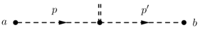
Figure 3: The Feynman–diagrammatic interpretation of the non-homogeneous free CTP propagator $i\Delta^{0,\,ab}(p,p^{\prime},\tilde{t}_{f};\tilde{t}_{i})$ for the real scalar $\Phi$, where the double line represents momentum-violating coupling to the thermal background through the bi-local source $K_{ab}(p,p^{\prime},\tilde{t}_{f};\tilde{t}_{i})$.

In (IV.3), the remaining terms linear in the external source $J$ yield contributions to the free propagator proportional to $K^{2}$ upon double functional differentiation with respect to $J$. As we shall see in Section V, these contributions may be neglected. Employing (59), we find that the non-homogeneous free CTP propagator $\Delta^{0,\,ab}(p,p^{\prime},\tilde{t}_{f};\tilde{t}_{i})$ may be expressed in terms of the free vacuum CTP propagator $\widehat{\Delta}^{0,\,ab}(p)$ and the bi-local source $K_{ab}(p,p^{\prime},\tilde{t}_{f};\tilde{t}_{i})$ as follows:

$$i\Delta^{0,\,ab}(p,p^{\prime},\tilde{t}_{f};\tilde{t}_{i})\ =\ i\widehat{\Delta}^{0,\,ab}(p)(2\pi)^{4}\delta^{(4)}(p\>-\>p^{\prime})\>+\>i\widehat{\Delta}^{0,\,ac}(p)iK_{cd}(p,p^{\prime},\tilde{t}_{f};\tilde{t}_{i})i\widehat{\Delta}^{0,\,db}(p^{\prime})\;,$$ (160)

where

$$K_{ab}(p,p^{\prime},\tilde{t}_{f};\tilde{t}_{i})\ =\ e^{i(p_{0}\>-\>p_{0}^{\prime})\tilde{t}_{f}}\,K_{ab}(\mathbf{p},\mathbf{p}^{\prime},t)\;.$$ (161)

The form of the free CTP propagator $\Delta^{0,\,ab}(p,p^{\prime},\tilde{t}_{f};\tilde{t}_{i})$ in (160) is consistent with a perturbative inversion of (120) to leading order in the bi-local source $K_{ab}$. It is also consistent with the canonically derived form of the non-homogeneous free propagators in (151).

The result in (160) may be interpreted diagrammatically, where the non-homogeneous free CTP propagator $i\Delta^{0,\,ab}(p,p^{\prime},\tilde{t}_{f};\tilde{t}_{i})$ for the real scalar $\Phi$ is associated with the Feynman diagram displayed in Figure 3. The bi-local source $K_{ab}(p,p^{\prime},\tilde{t}_{f};\tilde{t}_{i})$ plays the role of a three-momentum-violating vertex that gives rise to the violation of translational invariance, thus encoding the spatial inhomogeneity of the background.

V The Thermodynamic Equilibrium Limit

In this section, we derive the analytical forms of the free and resummed CTP propagators in the limit of thermal equilibrium. The results of this section are of particular importance for the discussion of pinch singularities in Section VIII. We also show the connection between the equilibrium Bose–Einstein distribution function and the bi-local source $K_{ab}$ introduced in Section IV.3.

In the limit of thermal equilibrium, the density operator $\rho$ is diagonal in particle number, so all amplitudes except $W_{11}$ vanish in (IV.3). In this limit, the general density operator $\rho$, given explicitly in (D), reduces to the series

$$\rho\ =\ \ket{0}\!\bra{0}\>+\>\!\iint\!\mathrm{d}{\Pi_{\mathbf{k}_{1}}}\,\mathrm{d}{\Pi_{\mathbf{k}_{1}^{\prime}}}\;\Big{(}\,(2\pi)^{3}2E(\mathbf{k}_{1})\delta^{(3)}(\mathbf{k}_{1}\>-\>\mathbf{k}_{1}^{\prime})\>-\>W_{11}(\mathbf{k}_{1}:\mathbf{k}_{1}^{\prime})$$

$$\qquad\qquad+\>\frac{1}{2}\!\int\!\mathrm{d}{\Pi_{\mathbf{q}_{1}}}\;W_{11}(\mathbf{k}_{1}:\mathbf{q}_{1})W_{11}(\mathbf{q}_{1}:\mathbf{k}_{1}^{\prime})\>+\>\cdots\,\Big{)}\!\ket{\mathbf{k}_{1}}\!\bra{\mathbf{k}_{1}^{\prime}}$$

$$\qquad+\>\frac{1}{2}\!\idotsint\!\mathrm{d}{\Pi_{\mathbf{k}_{1}}}\,\mathrm{d}{\Pi_{\mathbf{k}_{2}}}\,\mathrm{d}{\Pi_{\mathbf{k}_{1}^{\prime}}}\,\mathrm{d}{\Pi_{\mathbf{k}_{2}^{\prime}}}\;\Big{(}\,(2\pi)^{3}2E(\mathbf{k}_{1})\delta^{(3)}(\mathbf{k}_{1}\>-\>\mathbf{k}_{1}^{\prime})\>-\>W_{11}(\mathbf{k}_{1}:\mathbf{k}_{1}^{\prime})$$

$$\qquad\qquad+\>\frac{1}{2}\!\int\!\mathrm{d}{\Pi_{\mathbf{q}_{1}}}\;W_{11}(\mathbf{k}_{1}:\mathbf{q}_{1})W_{11}(\mathbf{q}_{1}:\mathbf{k}_{1}^{\prime})\>+\>\cdots\,\Big{)}\Big{(}\,(2\pi)^{3}2E(\mathbf{k}_{2})\delta^{(3)}(\mathbf{k}_{2}\>-\>\mathbf{k}_{2}^{\prime})$$

$$\qquad\qquad-\>W_{11}(\mathbf{k}_{2}:\mathbf{k}_{2}^{\prime})\>+\>\frac{1}{2}\!\int\!\mathrm{d}{\Pi_{\mathbf{q}_{2}}}\;W_{11}(\mathbf{k}_{2}:\mathbf{q}_{2})W_{11}(\mathbf{q}_{2}:\mathbf{k}_{2}^{\prime})\>+\>\cdots\,\Big{)}\!\ket{\mathbf{k}_{1},\mathbf{k}_{2}}\!\bra{\mathbf{k}_{1}^{\prime},\mathbf{k}_{2}^{\prime}}\>+\>\cdots\;,$$ (162)

where the time arguments in the multi-mode Fock states have been omitted for notational convenience. In the equilibrium limit, the statistical distribution function $g(\mathbf{p},\mathbf{p}^{\prime},t)$ is trivially zero. Instead, $f(\mathbf{p},\mathbf{p}^{\prime},t)$ is calculated from (143) and takes the form of the series

$$2\mathcal{E}(\mathbf{p},\mathbf{p}^{\prime})f(\mathbf{p},\mathbf{p}^{\prime},t)\ =\ (2\pi)^{3}2E(\mathbf{p})\delta^{(3)}(\mathbf{p}\>-\>\mathbf{p}^{\prime})\>-\>W_{11}(\mathbf{p}:\mathbf{p}^{\prime})\>+\>\frac{1}{2}\!\int\!\mathrm{d}{\Pi_{\mathbf{q}}}\;W_{11}(\mathbf{p}:\mathbf{q})W_{11}(\mathbf{q}:\mathbf{p}^{\prime})\>+\>\cdots$$

$$\qquad+\>\!\int\!\mathrm{d}{\Pi_{\mathbf{q}}}\;\Big{(}\,(2\pi)^{3}2E(\mathbf{p})\delta^{(3)}(\mathbf{p}\>-\>\mathbf{q})\>-\>W_{11}(\mathbf{p}:\mathbf{q})\>+\>\cdots\,\Big{)}$$

$$\qquad\quad\quad\times\>\Big{(}\,(2\pi)^{3}2E(\mathbf{q})\delta^{(3)}(\mathbf{q}\>-\>\mathbf{p}^{\prime})\>-\>W_{11}(\mathbf{q}:\mathbf{p}^{\prime})\>+\>\cdots\,\Big{)}\>+\>\cdots\;,$$ (163)

where disconnected parts have been canceled order-by-order in the expansion by the normalization $\mathrm{Tr}\,\rho$ in (93). The factor $\mathcal{E}(\mathbf{p},\mathbf{p}^{\prime})$ is defined in (144).

The equilibrium density operator $\rho_{\rm eq}$ must also be diagonal in the momenta and is thus obtained by making the replacement:

$$W_{11}(\mathbf{k}:\mathbf{k}^{\prime})\ \to\ \beta E(\mathbf{k})(2\pi)^{3}2E(\mathbf{k})\delta^{(3)}(\mathbf{k}\>-\>\mathbf{k}^{\prime})$$ (164)

in (V), where $\beta\>=\>1/T$ is the inverse thermodynamic temperature. In detail, we find

$$\rho_{\rm eq}\ =\ \ket{0}\!\bra{0}\>+\>\sum_{n=1}^{\infty}\frac{1}{n!}\!\idotsint\!\prod_{i=1}^{n}\Big{(}\,\mathrm{d}{\Pi_{\mathbf{k}_{i}}}\,f_{\beta}(\mathbf{k}_{i})\,\Big{)}\bigotimes_{i=1}^{n}\ket{\mathbf{k}_{i}}\bigotimes_{i=1}^{n}\bra{\mathbf{k}_{i}}\;,$$ (165)

where the amplitudes are the Boltzmann distributions $f_{\beta}(\mathbf{k})\>=\>e^{-\beta E(\mathbf{k})}$ [cf. (168)]. This last expression of $\rho_{\rm eq}$ can be shown to be fully equivalent to the Gaussian form

$$\rho_{\rm eq}\ =\ \exp\!\bigg{(}-\beta\!\int\!\mathrm{d}{\Pi_{\mathbf{k}}}\,E(\mathbf{k})a^{{\dagger}}(\mathbf{k})a(\mathbf{k})\bigg{)}\;,$$ (166)

which corresponds to the standard Boltzmann density operator

$$\rho_{\rm eq}\ =\ e^{-\beta H^{0}}\;,$$ (167)

where $H^{0}$ is the free part of the interaction-picture Hamiltonian. Note that our convention for the normalization of the density operator $\rho$, including $\rho_{\rm eq}$, is chosen so that the canonical partition function $\mathcal{Z}(\beta)\>=\>\mathrm{Tr}\,e^{-\beta H^{0}}$ appears explicitly in the definition of the EEV in (93).

We may now substitute the limit (164) into the series expansion of the statistical distribution function $f$ in (V). Using the identities of summation

$$\sum_{n=0}^{\infty}\frac{(-x)^{n}}{n!}\ =\ e^{-x}\;,\qquad\sum_{n=1}^{\infty}x^{n}\ =\ \frac{x}{1-x}\;,$$ (168)

we find the following correspondence in the equilibrium limit:

$$f(\mathbf{p},\mathbf{p}^{\prime},t) \ \underset{\mathrm{eq.}}{\longrightarrow}\ f_{\mathrm{eq}}(\mathbf{p},\mathbf{p}^{\prime})\ =\ (2\pi)^{3}\delta^{(3)}(\mathbf{p}\>-\>\mathbf{p}^{\prime})f_{\mathrm{B}}\big{(}E(\mathbf{p})\big{)}\;,$$ (169a)

$$g(\mathbf{p},\mathbf{p}^{\prime},t) \ \underset{\mathrm{eq.}}{\longrightarrow}\ g_{\mathrm{eq}}(\mathbf{p},\mathbf{p}^{\prime})\ =\ 0\;,$$ (169b)

where

$$f_{\mathrm{B}}(p_{0})\ =\ \frac{1}{e^{\beta p_{0}}\>-\>1}$$ (170)

is the Bose–Einstein distribution function. The equilibrium statistical distribution functions in (169) depend only on the magnitude of the three-momentum $\mathbf{p}$ via the on-shell energy $E(\mathbf{p})$. This is a consequence of the homogeneity and isotropy implied by thermodynamic equilibrium. Moreover, the multiplying factor $\delta^{(3)}(\mathbf{p}\>-\>\mathbf{p}^{\prime})$ on the RHS of (169) necessarily restores translational and rotational invariance.

It is well-known that the pinch singularities present in perturbative expansions cancel in the equilibrium limit Landsman and van Weert (1987) (see Section VIII) and we can safely take the limit $t\>\to\>\infty$ throughout the CTP generating functional, as we should expect for a system with static macroscopic properties. Working then in the single momentum representation, we obtain from (76) and (77) the free equilibrium CTP propagators

$$i\Delta^{0}_{\mathrm{F}}(p) \ =\ \Big{(}i\Delta_{\rm D}^{0}(p)\Big{)}^{*}\ =\ i\Big{(}p^{2}\>-\>M^{2}\>+\>i\varepsilon\Big{)}^{-1}\>+\>2\pi f_{\mathrm{B}}(|p_{0}|)\delta(p^{2}\>-\>M^{2})\;,$$ (171a)

$$i\Delta^{0}_{>}(p) \ =\ 2\pi\Big{(}\theta(p_{0})\>+\>f_{\mathrm{B}}(|p_{0}|)\Big{)}\delta(p^{2}\>-\>M^{2})\ \equiv\ 2\pi\varepsilon(p_{0})\Big{(}1\>+\>f_{\mathrm{B}}(p_{0})\Big{)}\delta(p^{2}\>-\>M^{2})\;,$$ (171b)

$$i\Delta^{0}_{<}(p) \ =\ 2\pi\Big{(}\theta(-p_{0})\>+\>f_{\mathrm{B}}(|p_{0}|)\Big{)}\delta(p^{2}-M^{2})\ \equiv\ 2\pi\varepsilon(p_{0})f_{\mathrm{B}}(p_{0})\delta(p^{2}\>-\>M^{2})\;.$$ (171c)

The form of the Wightman propagators written in terms of the signum function $\varepsilon(p_{0})$ prove very useful in the calculation of loop diagrams, as detailed in Appendix B.

Returning to the free CTP generating functional ${\cal Z}$ in (IV.3), it follows from the results above that in equilibrium the bi-local source $K_{ab}(p,p^{\prime},\tilde{t}_{f};\tilde{t}_{i})$ must be proportional to a four-dimensional delta function of the momenta, i.e.

$$K_{ab}(p,p^{\prime},\tilde{t}_{f};\tilde{t}_{i})\ \underset{\mathrm{eq.}}{\longrightarrow}\ K_{ab}^{\mathrm{eq}}(p,p^{\prime})\ =\ (2\pi)^{4}\delta^{(4)}(p\>-\>p^{\prime})K^{\mathrm{eq}}_{ab}(p)\;.$$ (172)

In addition, $K^{\mathrm{eq}}_{ab}(p)$ must satisfy

$$\widehat{\Delta}^{0,\,ac}(p)K^{\mathrm{eq}}_{cd}(p)\widehat{\Delta}^{0,\,db}(p)\ =\ 2\pi i\,\delta(p^{2}\>-\;M^{2})f_{\mathrm{B}}\big{(}E(\mathbf{p})\big{)}\!\begin{bmatrix}1&1\\ 1&1\end{bmatrix}\!\;.$$ (173)

Solving the resulting system of equations, keeping terms to leading order in $\epsilon$, and noting that $K^{\mathrm{eq}}_{ab}(p)$ should be written in terms of the three-momentum only, we find

$$K^{\mathrm{eq}}_{ab}(p)\ =\ 2i\epsilon f_{\mathrm{B}}\big{(}E(\mathbf{p})\big{)}\!\begin{bmatrix}1&-1\\ -1&1\end{bmatrix}\!\;.$$ (174)

By virtue of the limit representation of the delta function

$$\delta(x)\ =\ \lim_{\epsilon\>\to\>0}\,\frac{1}{\pi}\,\frac{\epsilon}{x^{2}\>+\>\epsilon^{2}}\;,$$ (175)

we can verify that we do indeed recover (173) and the correct free CTP propagator by means of (160). We also confirm that the terms linear in $J$ remaining in (IV.3) may safely be ignored, since they yield contributions to the free propagator proportional to $K^{2}\>\sim\>\epsilon^{2}$ upon double functional differentiation with respect to $J$.

Alternatively, interpreting the Boltzmann density operator in (167) as an evolution operator in negative imaginary time and using the cyclicity of the trace in the EEV, we derive the Kubo–Martin–Schwinger (KMS) relation (see for instance Le Bellac (2000))

$$\Delta_{>}(x^{0}-y^{0},\mathbf{x}-\mathbf{y})\ =\ \Delta_{<}(x^{0}-y^{0}+i\beta,\mathbf{x}-\mathbf{y})\;.$$ (176)

In the momentum representation, the KMS relation reads:

$$\Delta_{>}(p)\ =\ e^{\beta p_{0}}\Delta_{<}(p)\;,$$ (177)

which offers the final constraint on $\tilde{f}(p)$ in (77):

$$\tilde{f}(p)\ =\ \theta(p_{0})f_{\mathrm{B}}(p_{0})+\theta(-p_{0})f_{\mathrm{B}}(-p_{0})\ =\ f_{\mathrm{B}}(|p_{0}|)\;.$$ (178)

Furthermore, the KMS relation also leads to the fluctuation-dissipation theorem

$$\Delta_{1}(p)\ =\ \Big{(}\,1\>+\>2f_{\mathrm{B}}(p_{0})\Big{)}\,\Delta(p)\;,$$ (179)

relating the causality and unitarity relations in (24) and (28). Subsequently, by means of the KMS relation, we may write all propagators in terms of the retarded propagator $\Delta_{\mathrm{R}}(p)$:

$$\mathrm{Re}\,\Delta_{\mathrm{F}}(p) \ =\ \mathrm{Re}\,\Delta_{\mathrm{R}}(p)\;,$$ (180a)

$$\mathrm{Im}\,\Delta_{\mathrm{F}}(p) \ =\ \varepsilon(p_{0})\Big{(}1\>+\>2f_{\mathrm{B}}(|p_{0}|)\Big{)}\mathrm{Im}\,\Delta_{\mathrm{R}}(p)\;,$$ (180b)

$$\Delta_{>}(p) \ =\ 2i\varepsilon(p_{0})\Big{(}\theta(p_{0})\>+\>f_{\mathrm{B}}(|p_{0}|)\Big{)}\mathrm{Im}\,\Delta_{\mathrm{R}}(p)\;,$$ (180c)

$$\Delta_{<}(p) \ =\ 2i\varepsilon(p_{0})\Big{(}\theta(-p_{0})\>+\>f_{\mathrm{B}}(|p_{0}|)\Big{)}\mathrm{Im}\,\Delta_{\mathrm{R}}(p)\;.$$ (180d)

In the homogeneous equilibrium limit of the Schwinger–Dyson equation in (119), the inverse resummed CTP propagator is given by

$$\Delta^{-1}_{ab}(p)\ =\ \Delta_{ab}^{0,\,-1}(p)\>+\>\Pi_{ab}(p)\;.$$ (181)

In the absence of self-energy effects, the free equilibrium CTP propagator is obtained by inverting the equilbrium limit of (120):

$$D^{0,\,-1}_{ab}(p)\ =\ \Delta^{0,\,-1}_{ab}(p)\>+\>K_{ab}^{\mathrm{eq}}(p)\;.$$ (182)

Knowing that $K^{\mathrm{eq}}_{ab}\>\sim\>\epsilon$ from (174), the inversion of (182) can be done perturbatively to leading order in $K^{\mathrm{eq}}_{ab}(p)$, in which case the expression (160) gets reproduced. Beyond the tree-level, however, the contribution from the bi-local source $K^{\mathrm{eq}}_{ab}(p)$ may be neglected next to the self-energy term $\Pi_{ab}(p)$ and the inverse resummed CTP propagator is explicitly given by

$$\Delta_{ab}^{-1}(p)\ =\ \begin{bmatrix}p^{2}\>-\>M^{2}\>+\>\Pi(p)&-\Pi_{<}(p)\\ -\Pi_{>}(p)&-p^{2}\>+\>M^{2}\>-\>\Pi^{*}(p)\end{bmatrix}\!\;.$$ (183)

In this equilibrium limit, (183) may be inverted exactly, yielding the equilibrium resummed CTP propagator

$$\Delta^{ab}(p)\ =\ \Big{[}\,\Big{(}\,p^{2}\>-\>M^{2}\>+\>\mathrm{Re}\,\Pi_{\mathrm{R}}(p)\,\Big{)}^{2}\>+\>\Big{(}\,\mathrm{Im}\,\Pi_{\mathrm{R}}(p)\,\Big{)}^{2}\,\Big{]}^{-1}\begin{bmatrix}p^{2}\>-\>M^{2}\>+\>\Pi^{*}(p)&-\Pi_{<}(p)\\ -\Pi_{>}(p)&-p^{2}\>+\>M^{2}\>-\>\Pi(p)\end{bmatrix}\!\;.$$ (184)

The results obtained above in (184) may only be compared with existing resummations, see for instance Altherr (1995); Garbrecht and Garny (2012), in the thermodynamic equilibrium limit, as we have discussed in Sections IV.1 and IV.2.

In this single momentum representation, the self-energies satisfy the unitarity and causality relations

$$\Pi_{1}(p)\ =\ \Pi_{>}(p)\>+\>\Pi_{<}(p) \ =\ \Pi(p)\>-\>\Pi^{*}(p)\ =\ 2i\mathrm{Im}\,\Pi(p)\;,$$ (185a)

$$2iM\Gamma(p)\ =\ \Pi_{>}(p)\>-\>\Pi_{<}(p) \ =\ \Pi_{\mathrm{R}}(p)\>-\>\Pi_{\mathrm{A}}(p)\ =\ 2i\mathrm{Im}\,\Pi_{\mathrm{R}}(p)\;,$$ (185b)

where $\Gamma(p)$ is the Breit–Wigner width, relating the absorptive part of the retarded self-energy $\Pi_{\mathrm{R}}(p)$ to physical reaction rates Kobes (1991); van Eijck and van Weert (1992). Notice that the KMS relation (176) leads also to the detailed balance condition

$$\Pi_{>}(p)\ =\ e^{\beta p_{0}}\,\Pi_{<}(p)\;.$$ (186)

Given the relations in (185), we find, in compliance with (180), an analogous set of relations for the elements of the CTP self-energy:

$$\mathrm{Re}\,\Pi(p) \ =\ \mathrm{Re}\,\Pi_{\mathrm{R}}(p)\;,$$ (187a)

$$\mathrm{Im}\,\Pi(p) \ =\ \varepsilon(p_{0})\Big{(}1\>+\>2f_{\mathrm{B}}(|p_{0}|)\Big{)}\mathrm{Im}\,\Pi_{\mathrm{R}}(p)\;,$$ (187b)

$$\Pi_{>}(p) \ =\ 2i\varepsilon(p_{0})\Big{(}\theta(p_{0})\>+\>f_{\mathrm{B}}(|p_{0}|)\Big{)}\mathrm{Im}\,\Pi_{\mathrm{R}}(p)\;,$$ (187c)

$$\Pi_{<}(p) \ =\ 2i\varepsilon(p_{0})\Big{(}\theta(-p_{0})\>+\>f_{\mathrm{B}}(|p_{0}|)\Big{)}\mathrm{Im}\,\Pi_{\mathrm{R}}(p)\;.$$ (187d)

Ignoring the dispersive parts of the self-energy, we expect to recover the free CTP propagators given in (171) in the limit $\mathrm{Im}\,\Pi(p)\>\to\>\epsilon\>=\>0^{+}$. This limit is equivalent to

$$\mathrm{Im}\,\Pi_{\mathrm{R}}(p)\ \to\ \epsilon_{\mathrm{R}}\ \equiv\ \varepsilon(p_{0})\,\epsilon\;.$$ (188)

Expressing the equilibrium resummed CTP propagator in (184) in terms of the retarded absorptive self-energy $\mathrm{Im}\,\Pi_{\mathrm{R}}(p)$, we can convince ourselves that we do indeed reproduce the free equilibrium CTP propagators (171) in the limit (188).

In Appendix B, we discuss the correspondence of the results of this section with the Imaginary Time Formalsim (ITF), clarifying the analytic continuation of the imaginary-time propagator and self-energy.

VI The Particle Number Density

It is important to establish a direct connection between off-shell Green’s functions and physical observables. Such observables include the particle number density for which various interpretations have been reported in the literature Aarts and Berges (2001); Juchem et al. (2004); Prokopec et al. (2004a, b); Berges (2005); Lindner and Müller (2006); De Simone and Riotto (2007); Cirigliano et al. (2008); Garny et al. (2010); Cirigliano et al. (2010); Beneke et al. (2011); Anisimov et al. (2011). In this section, we derive a physically meaningful definition of the particle number density in terms of the resummed CTP propagators.

In order to count off-shell contributions systematically, we suggest to ‘measure’ the particle number density in terms of charges, rather than by quanta of energy. The latter approach would necessitate the use of a quasi-particle approximation to identify ‘single-particle’ energies, which we do not follow here. Instead, we analytically continue the real scalar field to a pair of complex scalar fields ($\Phi,\ \Phi^{{\dagger}}$). We may then introduce the Noether charge $\mathcal{Q}(x_{0};\tilde{t}_{i})$ of the global $U(1)$ symmetry for the Heisenberg-picture field $\Phi_{\mathrm{H}}(x;\tilde{t}_{i})$ operator:

$$\mathcal{Q}(x_{0};\tilde{t}_{i})\ =\ i\!\int\!\mathrm{d}^{3}{\mathbf{x}}\;\Big{(}\,\Phi_{\mathrm{H}}^{{\dagger}}(x;\tilde{t}_{i})\pi_{\mathrm{H}}^{{\dagger}}(x;\tilde{t}_{i})\>-\>\pi_{\mathrm{H}}(x;\tilde{t}_{i})\Phi_{\mathrm{H}}(x;\tilde{t}_{i})\,\Big{)}\;.$$ (189)

Here, $\pi_{\mathrm{H}}(x;\tilde{t}_{i})\>=\>\partial_{x_{0}}\Phi_{\mathrm{H}}^{{\dagger}}(x;\tilde{t}_{i})$ is the conjugate momentum operator and we include all time dependencies explicitly for clarity. In the absence of derivative interactions, the Noether charge depends only on the quadratic form of the kinetic term in the Lagrangian. Hence, this analytic continuation may be employed even for real scalar theories with interaction terms that break the $\mathbb{Z}_{2}$ symmetry. Up to the infinite $T\>=\>0$ vacuum contribution, the EEV of the operator $\mathcal{Q}(x_{0};\tilde{t}_{i})$ in (189) is zero on analytically continuing back to the original real scalar field $\Phi$, since the identical particle and anti-particle contributions cancel. Therefore, we need to devise a method by which to separate the particle from the anti-particle degrees of freedom in the EEV of (189).

We note that the Noether charge of the local $U(1)$ symmetry of the complex scalar theory is gauge-dependent and therefore unphysical. The physical conserved matter charge remains that of the global $U(1)$ symmetry and is recovered in the temporal gauge $A^{0}\>=\>0$. In this case, the conserved charge in (189) would be written in terms of the fields and their time derivatives and not the conjugate momenta of the full Lagrangian.

For the general case of a spatially and temporally inhomogeneous background, we need to generalize the Noether charge operator $\mathcal{Q}(x_{0};\tilde{t}_{i})$ by writing it in terms of a charge density operator $\mathcal{Q}(\mathbf{p},\mathbf{X},X_{0};\tilde{t}_{i})$ as

$$\mathcal{Q}(X_{0};\tilde{t}_{i})\ =\ \!\int\mathrm{d}^{3}{\mathbf{X}}\int\!\!\frac{\mathrm{d}^{3}{\mathbf{p}}}{(2\pi)^{3}}\;\mathcal{Q}(\mathbf{p},\mathbf{X},X_{0};\tilde{t}_{i})\;.$$ (190)

In the above, the three-momentum $\mathbf{p}$ is conjugate to the spatial part of the relative space-time coordinate $R^{\mu}\>=\>x^{\mu}\>-\>y^{\mu}$ and $X^{\mu}\>=\>(X^{0},\mathbf{X})\>=\>(x^{\mu}\>+\>y^{\mu})/2$ is the central space-time coordinate [cf. (33)]. To this end, we proceed by inserting into (189) unity in the following form:

$$1\ =\ \!\int\!\mathrm{d}^{4}{y}\;\delta^{(4)}(x\>-\>y)\ =\ \!\int\!\mathrm{d}^{4}{y}\int\!\!\frac{\mathrm{d}^{3}{\mathbf{p}}}{(2\pi)^{3}}\;e^{-i\mathbf{p}\cdot(\mathbf{x}\>-\>\mathbf{y})}\delta(x_{0}\>-\>y_{0})\;.$$ (191)

Observe that in what follows, $x^{0}\>=\>y^{0}\>=\>X^{0}$ thanks to $\delta(x_{0}\>-\>y_{0})$. Subsequently, symmetrizing the integrand in $x$ and $y$, we may write the charge operator as

$$\mathcal{Q}(X_{0};\tilde{t}_{i})\ =\ \frac{i}{2}\!\int\!\mathrm{d}^{3}{\mathbf{x}}\int\!\mathrm{d}^{4}{y}\!\int\!\!\frac{\mathrm{d}^{3}{\mathbf{p}}}{(2\pi)^{3}}\;e^{-i\mathbf{p}\cdot(\mathbf{x}\>-\>\mathbf{y})}\delta(x_{0}\>-\>y_{0})\Big{(}\,\Phi_{\mathrm{H}}^{{\dagger}}(y;\tilde{t}_{i})\pi_{\mathrm{H}}^{{\dagger}}(x;\tilde{t}_{i})\>-\>\pi_{\mathrm{H}}(y;\tilde{t}_{i})\Phi_{\mathrm{H}}(x;\tilde{t}_{i})\>+\>(x\>\leftrightarrow\>y)\,\Big{)}\;.$$ (192)

In terms of the central and relative coordinates, $X^{\mu}$ and $R^{\mu}$, the charge density operator $\mathcal{Q}(\mathbf{p},\mathbf{X},X_{0};\tilde{t}_{i})$ may be appropriately identified from (192) as

$$\mathcal{Q}(\mathbf{p},\mathbf{X},X_{0};\tilde{t}_{i})\ =\ \frac{i}{2}\!\int\!\mathrm{d}^{4}{R}\;e^{-i\mathbf{p}\cdot\mathbf{R}}\,\delta(R_{0})\Big{(}\,\Phi_{\mathrm{H}}^{{\dagger}}(X-\tfrac{R}{2};\tilde{t}_{i})\pi_{\mathrm{H}}^{{\dagger}}(X+\tfrac{R}{2};\tilde{t}_{i})\>-\>\pi_{\mathrm{H}}(X-\tfrac{R}{2};\tilde{t}_{i})\Phi_{\mathrm{H}}(X+\tfrac{R}{2};\tilde{t}_{i})\>+\>(R\>\leftrightarrow\>-R)\,\Big{)}\;.$$ (193)

Substituting for the definitions of the conjugate-momentum operators $\pi_{\mathrm{H}}$ and $\pi_{\mathrm{H}}^{{\dagger}}$, we may rewrite $\mathcal{Q}(\mathbf{p},\mathbf{X},X_{0};\tilde{t}_{i})$ in the following form:

$$\mathcal{Q}(\mathbf{p},\mathbf{X},X_{0};\tilde{t}_{i})\ =\ i\!\int\!\mathrm{d}^{4}{R}\;e^{-i\mathbf{p}\cdot\mathbf{R}}\,\delta(R_{0})\partial_{R_{0}}\Big{(}\Phi_{\mathrm{H}}^{{\dagger}}(X-\tfrac{R}{2};\tilde{t}_{i})\Phi_{\mathrm{H}}(X+\tfrac{R}{2};\tilde{t}_{i})\>-\>\Phi_{\mathrm{H}}^{{\dagger}}(X+\tfrac{R}{2};\tilde{t}_{i})\Phi_{\mathrm{H}}(X-\tfrac{R}{2};\tilde{t}_{i})\Big{)}\;.$$ (194)

The EEV of $\mathcal{Q}(\mathbf{p},\mathbf{X},X_{0};\tilde{t}_{i})$ at the macroscopic time $t$ is then obtained by taking the trace with the density operator $\rho$ as given in (93) in the equal-time limit $X_{0}\>=\>\tilde{t}_{f}$. We have seen in Section III that the equal-time limit is necessary to ensure that the observable charge density is picture independent and that the number of independent coordinates is reduced to seven as required. Thus, we have

$$\braket{\mathcal{Q}(\mathbf{p},\mathbf{X},\tilde{t}_{f};\tilde{t}_{i})}_{t}\ =\ \lim_{X_{0}\>\to\>\tilde{t}_{f}}\,i\!\int\!\mathrm{d}^{4}{R}\;e^{-i\mathbf{p}\cdot\mathbf{R}}\,\delta(R_{0})\partial_{R_{0}}\Big{(}\,i\Delta_{<}(R,X,\tilde{t}_{f};\tilde{t}_{i})\>-\>i\Delta_{<}(-R,X,\tilde{t}_{f};\tilde{t}_{i})\,\Big{)}\;,$$ (195)

where we use the notation

$$i\Delta_{<}(R,X,\tilde{t}_{f};\tilde{t}_{i})\ =\ \braket{\Phi_{\mathrm{H}}^{{\dagger}}(X-\tfrac{R}{2};\tilde{t}_{i})\Phi_{\mathrm{H}}(X+\tfrac{R}{2};\tilde{t}_{i})}_{t}$$ (196)

for the resummed CTP Wightman propagator.

Let us comment on the two terms $i\Delta_{<}(R,X,\tilde{t}_{f};\tilde{t}_{i})$ and $i\Delta_{<}(-R,X,\tilde{t}_{f};\tilde{t}_{i})$ that occur on the RHS of (195). The first term $i\Delta_{<}(R,X,\tilde{t}_{f};\tilde{t}_{i})$ comprises ensemble positive-frequency particle modes and ensemble plus vacuum negative-frequency anti-particle modes. The second one $i\Delta_{<}(-R,X,\tilde{t}_{f};\tilde{t}_{i})$ comprises ensemble plus vacuum positive-frequency anti-particle modes and ensemble negative-frequency particle modes. Hence, we may extract the number density of particles by taking the sum of the positive-frequency contribution from $i\Delta_{<}(R,X,\tilde{t}_{f};\tilde{t}_{i})$ and the negative-frequency contribution from $i\Delta_{<}(-R,X,\tilde{t}_{f};\tilde{t}_{i})$.

We separate the positive- and negative-frequency parts of (195) by decomposing the equal-time delta function $\delta(R_{0})$ via the limit representation

$$\delta(R_{0})\ =\ \frac{i}{2\pi}\bigg{(}\frac{1}{R_{0}\>+\>i\epsilon}\>-\>\frac{1}{R_{0}\>-\>i\epsilon}\bigg{)}\;,$$ (197)

with $\epsilon=0^{+}$. Thus, a physically meaningful definition of the number density of particles at the macroscopic time $t$ is given by

$$n(\mathbf{p},\mathbf{X},\tilde{t}_{f};\tilde{t}_{i})\ =\ -\lim_{X_{0}\>\to\>\tilde{t}_{f}}\,\!\int\!\mathrm{d}^{3}{\mathbf{R}}\;e^{-i\mathbf{p}\cdot\mathbf{R}}\int\!\frac{\mathrm{d}{R_{0}}}{2\pi}\bigg{(}\frac{1}{R_{0}\>+\>i\epsilon}\,\partial_{R_{0}}i\Delta_{<}(R,X,\tilde{t}_{f};\tilde{t}_{i})\>+\>\frac{1}{R_{0}\>-\>i\epsilon}\,\partial_{R_{0}}i\Delta_{<}(-R,X,\tilde{t}_{f};\tilde{t}_{i})\bigg{)}\;.$$ (198)

Using time translational invariance of the CTP contour, this observable may be recast in terms of the Wigner transform of the Wightman propagators as

$$n(\mathbf{p},\mathbf{X},t)\ \equiv\ n(\mathbf{p},\mathbf{X},t;0)\ =\ \lim_{X_{0}\>\to\>t}\,\!\int\!\frac{\mathrm{d}{p_{0}}}{2\pi}\;p_{0}\Big{(}\,\theta(p_{0})i\Delta_{<}(p,X,t;0)\>-\>\theta(-p_{0})i\Delta_{<}(-p,X,t;0)\,\Big{)}\;.$$ (199)

Note that the number density of anti-particles $n^{C}(\mathbf{p},\mathbf{X},t)$ is obtained by $C$-conjugating the two negative-frequency Wightman propagators in (199). Useful relations between correlation functions and their $C$-conjugated counterparts are given in Appendices A and C.

We reiterate from (146) that the $n(\mathbf{p},\mathbf{X},t)\,\mathrm{d}^{3}{\mathbf{p}}\,\mathrm{d}^{3}{\mathbf{X}}$ is interpreted as the number of particles at macroscopic time $t$ in the volume of phase space between $\mathbf{p}$ and $\mathbf{p}\>+\>\mathrm{d}{\mathbf{p}}$ and $\mathbf{X}$ and $\mathbf{X}\>+\>\mathrm{d}{\mathbf{X}}$. The particle number per unit volume is obtained by integrating over all momentum modes, i.e.

$$n(\mathbf{X},t)\ =\ \!\int\!\!\frac{\mathrm{d}^{3}{\mathbf{p}}}{(2\pi)^{3}}\;n(\mathbf{p},\mathbf{X},t)\;,$$ (200)

and finally the total particle number, by integrating over all space, i.e.

$$N(t)\ =\ \!\int\!\mathrm{d}^{3}{\mathbf{X}}\;n(\mathbf{X},t)\;.$$ (201)

By inserting the inverse Wigner transform

$$i\Delta_{<}(p,X,t;0)\ =\ \!\int\!\!\frac{\mathrm{d}^{4}{P}}{(2\pi)^{4}}\;e^{-iP\cdot X}\,i\Delta_{<}(p+\tfrac{P}{2},p-\tfrac{P}{2},t;0)\;,$$ (202)

into (199), the particle number per unit volume $n(\mathbf{X},t)$ may be expressed in terms of the double momentum representation of the Wightman propagators via (200). After making the coordinate transformation $p\>\to\>-\>p$ in the negative-frequency contribution, we then obtain

$$n(\mathbf{X},t)\ =\ \lim_{X_{0}\>\to\>t}\,2\!\iint\!\!\frac{\mathrm{d}^{4}{p}}{(2\pi)^{4}}\,\frac{\mathrm{d}^{4}{P}}{(2\pi)^{4}}\;e^{-iP\cdot X}\,\theta(p_{0})p_{0}i\Delta_{<}(p+\tfrac{P}{2},p-\tfrac{P}{2},t;0)\;,$$ (203)

The particle number per unit volume $n(\mathbf{X},t)$ in (203) is related to the statistical distribution function $f$, through

$$n(\mathbf{X},t)\ =\ \!\int\!\!\frac{\mathrm{d}^{3}{\mathbf{p}}}{(2\pi)^{3}}\int\!\!\frac{\mathrm{d}^{3}{\mathbf{P}}}{(2\pi)^{3}}\;e^{i\mathbf{P}\cdot\mathbf{X}}\,f(\mathbf{p}+\tfrac{\mathbf{P}}{2},\mathbf{p}-\tfrac{\mathbf{P}}{2},t)\;,$$ (204)

cf. (146). Here, we must emphasize that (204) is understood in the Heisenberg picture. Working instead in the interaction picture, (203) and (204) define the statistical distribution function at a given order in perturbation theory. Explicitly, the $n$-loop statistical distribution function is defined in terms of the $n$-loop negative-frequency Wightman propagator via

$$f^{(n)}(\mathbf{p}+\tfrac{\mathbf{P}}{2},\mathbf{p}-\tfrac{\mathbf{P}}{2},t)\ =\ \lim_{X_{0}\>\to\>t}\,2\!\iint\!\!\frac{\mathrm{d}{p_{0}}}{2\pi}\,\frac{\mathrm{d}{P_{0}}}{2\pi}\;e^{-iP_{0}X_{0}}\,\theta(p_{0})p_{0}i\Delta^{(n)}_{<}(p+\tfrac{P}{2},p-\tfrac{P}{2},t;0)\;.$$ (205)

It is instructive to check that our definitions for the number density lead to the expected results for the free and quasi-particle equilibrium cases. Substituting the free equilibrium Wightman propagator (171c) of the real scalar field into (199), we obtain

$$n^{0}_{\mathrm{eq}}(\mathbf{p},\mathbf{X},t)\ =\ f_{\mathrm{B}}\big{(}E(\mathbf{p})\big{)}\;,$$ (206)

exactly as we would expect for the number density of spectrally-free particles in thermodynamic equilibrium. Inserting instead the resummed equilibrium Wightman propagator given in (184) in the narrow width limit, we get

$$n_{\mathrm{qp}}(\mathbf{p},\mathbf{X},t)\ =\ f_{\mathrm{B}}\big{(}\mathcal{E}(\mathbf{p})\big{)}\;,$$ (207)

where $\mathcal{E}(\mathbf{p})$ is the solution to the gap equation,

$$\mathcal{E}^{2}(\mathbf{p})\ =\ \mathbf{p}^{2}\>+\>M^{2}\>-\>\mathrm{Re}\,\Pi_{\mathrm{R}}(\mathcal{E}(\mathbf{p})+i\epsilon,\mathbf{p})\;,$$ (208)

and $n_{\mathrm{qp}}(\mathbf{p},\mathbf{X},t)$ then represents the number density of quasi-particles.

VII Master Time Evolution Equations for Particle Number Densities

Having established a direct relationship between the non-homogeneous CTP propagators and the particle number density in Section VI, we are now in a position to derive in this section master time evolution equations for the particle number density $n({\bf X},t)$ and the statistical distribution function $f(\mathbf{p},\mathbf{p}^{\prime},t)$. This is achieved in analogy to the derivation of the well-known Kadanoff–Baym equations Baym and Kadanoff (1961); Kadanoff and Baym (1989) by partially inverting the CTP Schwinger–Dyson equation obtained in Section IV.1. Our approach, however, differs significantly from other methods in that we do not rely on a truncation of a gradient expansion of the resulting expressions. More details of the gradient expansion can be found in Section IV.2 and Appendix E. In the next section, we will employ a loopwise truncation of the time evolution equations in terms of non-homogeneous free CTP propagators. As we will see, these dynamical equations are nonetheless resummed to all orders in a gradient expansion.

We begin our derivation of the time evolution equations with the double momentum representation of the Schwinger–Dyson equation in (122). We convolute (122) consecutively from the right with the weight function $(2\pi)^{4}\delta_{t}^{(4)}(q_{1}\>-\>q_{2})$ defined in (83) and then with the resummed CTP propagator $\Delta^{ab}(q_{2},p_{2},\tilde{t}_{f};\tilde{t}_{i})$. By making use of the inverse relation (82), we obtain the following expression:

$$\iint\!\!\frac{\mathrm{d}^{4}{q_{1}}}{(2\pi)^{4}}\,\frac{\mathrm{d}^{4}{q_{2}}}{(2\pi)^{4}}\;\Delta_{ac}^{0,\,-1}(p_{1},q_{1})(2\pi)^{4}\delta_{t}^{(4)}(q_{1}\>-\>q_{2})\Delta^{c}_{\;b}(q_{2},p_{2},\tilde{t}_{f};\tilde{t}_{i})$$

$$\qquad=\ \eta_{ab}(2\pi)^{4}\delta^{(4)}_{t}(p_{1}\>-\>p_{2})\>-\>\!\iint\!\!\frac{\mathrm{d}^{4}{q_{1}}}{(2\pi)^{4}}\,\frac{\mathrm{d}^{4}{q_{2}}}{(2\pi)^{4}}\;\Pi_{ac}(p_{1},q_{1},\tilde{t}_{f};\tilde{t}_{i})(2\pi)^{4}\delta^{(4)}_{t}(q_{1}\>-\>q_{2})\Delta_{\;b}^{c}(q_{2},p_{2},\tilde{t}_{f};\tilde{t}_{i})\;,$$ (209)

where the contribution of the bi-local source $K_{ab}$ is neglected next to the self-energies. It is essential to remark that the LHS of (VII) has the following coordinate-space representation:

$$\int_{\Omega_{t}}\!\!\mathrm{d}^{4}{z}\;\Delta^{0,\,-1}_{ab}(x,z)\Delta^{b}_{\;c}(z,y,\tilde{t}_{f};\tilde{t}_{i})\;.$$ (210)

Substituting for the free inverse CTP propagator $\Delta^{0,\,-1}_{ab}(x,y)$ given in (55), we may then confirm via (210) that evaluating the $q_{1}$ and $q_{2}$ integrals on the LHS of (VII) yields

$$\iint\!\!\frac{\mathrm{d}^{4}{q_{1}}}{(2\pi)^{4}}\,\frac{\mathrm{d}^{4}{q_{2}}}{(2\pi)^{4}}\;\Delta_{ac}^{0,\,-1}(p_{1},q_{1})(2\pi)^{4}\delta_{t}^{(4)}(q_{1}\>-\>q_{2})\Delta^{c}_{\;b}(q_{2},p_{2},\tilde{t}_{f};\tilde{t}_{i})\ =\ \Big{(}\,p_{1}^{2}\>-\>M^{2}\,\Big{)}\Delta_{ab}(p_{1},p_{2},\tilde{t}_{f};\tilde{t}_{i})\;.$$ (211)

Recalling that the self-energy $\Pi_{ab}(p,p^{\prime},\tilde{t}_{f};\tilde{t}_{i})$ contains $\delta^{(4)}_{t}(p\>-\>p^{\prime})$ functions in the vertices, we may perform the $q_{1}$ integral on the RHS of (VII) by making use of (86). Consequently, (VII) may be written down in the following concise form:

$$\Big{(}\,p_{1}^{2}\>-\>M^{2}\,\Big{)}\Delta_{ab}(p_{1},p_{2},\tilde{t}_{f};\tilde{t}_{i})\ =\ \eta_{ab}(2\pi)^{4}\delta_{t}^{(4)}(p_{1}\>-\>p_{2})\>-\>\!\int\!\!\frac{\mathrm{d}^{4}{q}}{(2\pi)^{4}}\;\Pi_{ac}(p_{1},q,\tilde{t}_{f};\tilde{t}_{i})\Delta^{c}_{\;b}(q,p_{2},\tilde{t}_{f};\tilde{t}_{i})\;.$$ (212)

At this point, it is essential to remark that, in any loopwise truncation of (212), the external propagator $\Delta_{ab}(p,p^{\prime},\tilde{t}_{f};\tilde{t}_{i})$, appearing on both the left- and right-hand sides, must be evaluated at the same order. This constraint ensures that the delta function on the RHS of (212) is present order-by-order in such an expansion and that the convolution in (VII) remains self-consistent.

With the definition of the particle number per unit volume $n(\mathbf{X},t)$ from (200) in mind, we equate the element $(a,b)\>=\>(1,2)$ of each side of (212) to extract the interacting Klein–Gordon equation of the negative-frequency resummed Wightman propagator:

$$\Big{(}\,p_{1}^{2}\>-\>M^{2}\,\Big{)}\Delta_{<}(p_{1},p_{2},\tilde{t}_{f};\tilde{t}_{i})\ =\ -\!\int\!\!\frac{\mathrm{d}^{4}{q}}{(2\pi)^{4}}\;\Big{(}\,\Pi(p_{1},q,\tilde{t}_{f};\tilde{t}_{i})\Delta_{<}(q,p_{2},\tilde{t}_{f};\tilde{t}_{i})\>-\>\Pi_{<}(p_{1},q,\tilde{t}_{f};\tilde{t}_{i})\Delta_{\mathrm{D}}(q,p_{2},\tilde{t}_{f};\tilde{t}_{i})\,\Big{)}\;.$$ (213)

Using the decomposition of $\Delta_{\mathrm{D}}(p,p^{\prime},\tilde{t}_{f};\tilde{t}_{i})$ from (324e) and an analogous identity for $\Pi(p,p^{\prime},\tilde{t}_{f};\tilde{t}_{i})$, we may rewrite (213) as

$$\Big{(}\,p_{1}^{2}\>-\>M^{2}\,\Big{)}\Delta_{<}(p_{1},p_{2},\tilde{t}_{f};\tilde{t}_{i})\>+\>\!\int\!\!\frac{\mathrm{d}^{4}{q}}{(2\pi)^{4}}\;\Pi_{\mathcal{P}}(p_{1},q,\tilde{t}_{f};\tilde{t}_{i})\Delta_{<}(q,p_{2},\tilde{t}_{f};\tilde{t}_{i})$$

$$\qquad\qquad=\ -\frac{1}{2}\!\int\!\!\frac{\mathrm{d}^{4}{q}}{(2\pi)^{4}}\;\Big{[}\,\Pi_{>}(p_{1},q,\tilde{t}_{f};\tilde{t}_{i})\Delta_{<}(q,p_{2},\tilde{t}_{f};\tilde{t}_{i})\>-\>\Pi_{<}(p_{1},q,\tilde{t}_{f};\tilde{t}_{i})\,\Big{(}\,\Delta_{>}(q,p_{2},\tilde{t}_{f};\tilde{t}_{i})\>-\>2\Delta_{\mathcal{P}}(q,p_{2},\tilde{t}_{f};\tilde{t}_{i})\,\Big{)}\,\Big{]}\;,$$ (214)

where the subscript $\mathcal{P}$ denotes principal-part evaluation of the functions given in (29) and (117b).

Introducing the central and relative momenta, $p\>=\>(p_{1}\>+\>p_{2})/2$ and $P\>=\>p_{1}\>-\>p_{2}$, respectively, we write (VII) in the following form:

$$\Big{[}\,\big{(}\,p_{0}\>+\>\tfrac{P_{0}}{2}\big{)}^{2}\>-\>E^{2}(\mathbf{p}\>+\>\tfrac{\mathbf{P}}{2})\,\Big{]}\Delta_{<}(p+\tfrac{P}{2},p-\tfrac{P}{2},\tilde{t}_{f};\tilde{t}_{i})\>+\>\mathscr{F}(p+\tfrac{P}{2},p-\tfrac{P}{2},\tilde{t}_{f};\tilde{t}_{i})\ =\ \mathscr{C}(p+\tfrac{P}{2},p-\tfrac{P}{2},\tilde{t}_{f};\tilde{t}_{i})\;,$$ (215)

where we have defined

$$\mathscr{F}(p+\tfrac{P}{2},p-\tfrac{P}{2},\tilde{t}_{f};\tilde{t}_{i})\ \equiv\ -\!\int\!\!\frac{\mathrm{d}^{4}{q}}{(2\pi)^{4}}\;i\Pi_{\mathcal{P}}(p+\tfrac{P}{2},q,\tilde{t}_{f};\tilde{t}_{i})\>i\Delta_{<}(q,p-\tfrac{P}{2},\tilde{t}_{f};\tilde{t}_{i}),$$ (216a)

$$\mathscr{C}(p+\tfrac{P}{2},p-\tfrac{P}{2},\tilde{t}_{f};\tilde{t}_{i})\ \equiv\ \frac{1}{2}\!\int\!\!\frac{\mathrm{d}^{4}{q}}{(2\pi)^{4}}\;\Big{[}\,i\Pi_{>}(p+\tfrac{P}{2},q,\tilde{t}_{f};\tilde{t}_{i})\>i\Delta_{<}(q,p-\tfrac{P}{2},\tilde{t}_{f};\tilde{t}_{i})$$

$$\qquad-\>i\Pi_{<}(p+\tfrac{P}{2},q,\tilde{t}_{f};\tilde{t}_{i})\,\Big{(}\,i\Delta_{>}(q,p-\tfrac{P}{2},\tilde{t}_{f};\tilde{t}_{i})\>-\>2i\Delta_{\mathcal{P}}(q,p-\tfrac{P}{2},\tilde{t}_{f};\tilde{t}_{i})\,\Big{)}\,\Big{]}\;.$$ (216b)

With the aim of finding a master time evolution equation for the particle number density $n({\bf X},t)$ in (200), we integrate both sides of (215) with the measure

$$\iint\!\!\frac{\mathrm{d}^{4}{p}}{(2\pi)^{4}}\frac{\mathrm{d}^{4}{P}}{(2\pi)^{4}}\;e^{-iP\cdot X}\,\theta(p_{0})\;.$$ (217)

Explicitly, this gives

$$\iint\!\!\frac{\mathrm{d}^{4}{p}}{(2\pi)^{4}}\,\frac{\mathrm{d}^{4}{P}}{(2\pi)^{4}}\;e^{-iP\cdot X}\,\theta(p_{0})\Big{[}\,\big{(}p_{0}\>+\>\tfrac{P_{0}}{2}\big{)}^{2}\>-\>E^{2}(\mathbf{p}+\tfrac{\mathbf{P}}{2})\,\Big{]}\Delta_{<}(p+\tfrac{P}{2},p-\tfrac{P}{2},\tilde{t}_{f};\tilde{t}_{i})$$

$$\qquad+\>\!\iint\!\!\frac{\mathrm{d}^{4}{p}}{(2\pi)^{4}}\,\frac{\mathrm{d}^{4}{P}}{(2\pi)^{4}}\;e^{-iP\cdot X}\,\theta(p_{0})\,\mathscr{F}(p+\tfrac{P}{2},p-\tfrac{P}{2},\tilde{t}_{f};\tilde{t}_{i})\ =\ \!\iint\!\!\frac{\mathrm{d}^{4}{p}}{(2\pi)^{4}}\,\frac{\mathrm{d}^{4}{P}}{(2\pi)^{4}}\;e^{-iP\cdot X}\,\theta(p_{0})\,\mathscr{C}(p+\tfrac{P}{2},p-\tfrac{P}{2},\tilde{t}_{f};\tilde{t}_{i})\;.$$ (218)

Adding to (VII) the complex conjugate of the same expression with $P\>\to\>-P$ and using the identities in (322), we may extract the terms proportional to $p\cdot P$ on the LHS of (VII). In this way, we obtain

$$2\!\iint\!\!\frac{\mathrm{d}^{4}{p}}{(2\pi)^{4}}\,\frac{\mathrm{d}^{4}{P}}{(2\pi)^{4}}\;e^{-iP\cdot X}\,\theta(p_{0})\,p\cdot P\,\Delta_{<}(p+\tfrac{P}{2},p-\tfrac{P}{2},\tilde{t}_{f};\tilde{t}_{i})$$

$$\quad+\>\!\iint\!\!\frac{\mathrm{d}^{4}{p}}{(2\pi)^{4}}\,\frac{\mathrm{d}^{4}{P}}{(2\pi)^{4}}\;e^{-iP\cdot X}\,\theta(p_{0})\Big{(}\,\mathscr{F}(p+\tfrac{P}{2},p-\tfrac{P}{2},\tilde{t}_{f};\tilde{t}_{i})\>+\>\mathscr{F}^{*}(p-\tfrac{P}{2},p+\tfrac{P}{2},\tilde{t}_{f};\tilde{t}_{i})\,\Big{)}$$

$$\quad\quad=\ \!\iint\!\!\frac{\mathrm{d}^{4}{p}}{(2\pi)^{4}}\,\frac{\mathrm{d}^{4}{P}}{(2\pi)^{4}}\,e^{-iP\cdot X}\,\theta(p_{0})\Big{(}\,\mathscr{C}(p+\tfrac{P}{2},p-\tfrac{P}{2},\tilde{t}_{f};\tilde{t}_{i})\>+\>\mathscr{C}^{*}(p-\tfrac{P}{2},p+\tfrac{P}{2},\tilde{t}_{f};\tilde{t}_{i})\,\Big{)}\;.$$ (219)

The first term on the LHS of (VII) may be rewritten as

$$2\!\iint\!\!\frac{\mathrm{d}^{4}{p}}{(2\pi)^{4}}\,\frac{\mathrm{d}^{4}{P}}{(2\pi)^{4}}\;\theta(p_{0})\Big{(}\,ip_{0}\partial_{X_{0}}\>-\>\mathbf{p}\cdot\mathbf{P}\,\Big{)}e^{-iP\cdot X}\,\Delta_{<}(p+\tfrac{P}{2},p-\tfrac{P}{2},\tilde{t}_{f};\tilde{t}_{i})\;.$$ (220)

Using time translational invariance of the CTP contour and taking the limit $X_{0}\>\to\>t$ in (220), we recognize that the derivative term with respect to $t$ is precisely the time derivative of the particle number density $n(\mathbf{X},t)$ in (200). Hence, from (VII) and (220), we arrive at our master time evolution equation for $n(\mathbf{X},t)$:

$$\partial_{t}n(\mathbf{X},t)\>-\>2\!\iint\!\!\frac{\mathrm{d}^{4}{p}}{(2\pi)^{4}}\,\frac{\mathrm{d}^{4}{P}}{(2\pi)^{4}}\;e^{-iP\cdot X}\,\mathbf{p}\cdot\mathbf{P}\,\theta(p_{0})\Delta_{<}(p+\tfrac{P}{2},p-\tfrac{P}{2},t;0)$$

$$\qquad+\>\!\iint\!\!\frac{\mathrm{d}^{4}{p}}{(2\pi)^{4}}\,\frac{\mathrm{d}^{4}{P}}{(2\pi)^{4}}\;e^{-iP\cdot X}\,\theta(p_{0})\Big{(}\,\mathscr{F}(p+\tfrac{P}{2},p-\tfrac{P}{2},t;0)\>+\>\mathscr{F}^{*}(p-\tfrac{P}{2},p+\tfrac{P}{2},t;0)\,\Big{)}$$

$$\qquad\qquad=\ \!\iint\!\!\frac{\mathrm{d}^{4}{p}}{(2\pi)^{4}}\,\frac{\mathrm{d}^{4}{P}}{(2\pi)^{4}}\;e^{-iP\cdot X}\theta(p_{0})\Big{(}\,\mathscr{C}(p+\tfrac{P}{2},p-\tfrac{P}{2},t;0)\>+\>\mathscr{C}^{*}(p-\tfrac{P}{2},p+\tfrac{P}{2},t;0)\,\Big{)}\;,$$ (221)

with $X_{0}\>=\>t$, where $\mathscr{F}$ and $\mathscr{C}$ are defined in (216a) and (216). Comparing with the full non-truncated form of the Kadanoff–Baym kinetic equation in (383), the series of nested Poisson brackets in (383) has been replaced by a single convolution integral over the central momentum $P$ in (VII).

In addition to the master time evolution equation for the particle number density $n(\mathbf{X},t)$ in (VII), we may respectively find a time evolution equation for the statistical distribution function $f(\mathbf{p}+\tfrac{\mathbf{P}}{2},\mathbf{p}-\tfrac{\mathbf{P}}{2},t)$. Specifically, given the relation (204) and the differential equation (VII), the following time evolution equation may be derived for the resummed statistical distribution function $f$:

$$\partial_{t}f(\mathbf{p}+\tfrac{\mathbf{P}}{2},\mathbf{p}-\tfrac{\mathbf{P}}{2},t)\>-\>2\!\iint\!\frac{\mathrm{d}{p_{0}}}{2\pi}\,\frac{\mathrm{d}{P_{0}}}{2\pi}\;e^{-iP_{0}t}\,\mathbf{p}\cdot\mathbf{P}\,\theta(p_{0})\Delta_{<}(p+\tfrac{P}{2},p-\tfrac{P}{2},t;0)$$

$$\qquad+\>\!\iint\!\frac{\mathrm{d}{p_{0}}}{2\pi}\,\frac{\mathrm{d}{P_{0}}}{2\pi}\;e^{-iP_{0}t}\,\theta(p_{0})\Big{(}\,\mathscr{F}(p+\tfrac{P}{2},p-\tfrac{P}{2},t;0)\>+\>\mathscr{F}^{*}(p-\tfrac{P}{2},p+\tfrac{P}{2},t;0)\,\Big{)}$$

$$\qquad\qquad=\ \!\iint\!\frac{\mathrm{d}{p_{0}}}{2\pi}\,\frac{\mathrm{d}{P_{0}}}{2\pi}\;e^{-iP_{0}t}\,\theta(p_{0})\Big{(}\,\mathscr{C}(p+\tfrac{P}{2},p-\tfrac{P}{2},t;0)\>+\>\mathscr{C}^{*}(p-\tfrac{P}{2},p+\tfrac{P}{2},t;0)\,\Big{)}\;.$$ (222)

It is important to stress here that (VII) provides a self-consistent time evolution equation for $f$ valid to all orders in perturbation theory and to all orders in gradient expansion.

We note that a physical interpretation may be attributed to the different terms contributing to (VII). Specifically, all terms on the LHS of (VII) may be associated with the total derivative in the phase space $(\mathbf{X},\ \mathbf{p})$, appearing in the classical Boltzmann transport equation Kolb and Turner (1994):

$$D_{t}\ =\ \partial_{t}\>+\>\mathbf{v}\cdot\mathbf{\nabla}_{\mathbf{X}}\>+\>{\bf F}\cdot\mathbf{\nabla}_{\mathbf{p}}\;,$$ (223)

where $\mathbf{v}$ is the average non-relativistic velocity of the particle distribution and ${\bf F}$ is the force acting on this distribution. In particular, the $\mathscr{F}$ terms on the LHS of (VII) are the force terms, generated by the potential due to the dispersive part of the self-energy. On the RHS of (VII), the $\mathscr{C}$ terms represent the collision terms.

It would be interesting to discuss the spatially homogeneous limit of (VII) at late times. In this case, energy conservation holds to a good approximation, so the time-dependent weight functions $\delta_{t}$ may be replaced by the standard Dirac delta functions, even in the vertices of the self-energies contained in the force $\mathscr{F}$ and collision $\mathscr{C}$ terms of (VII). Moreover, as a consequence of the assumed spatial homogeneity, all propagators and self-energies, which in general depend on two momenta $p_{1}$ and $p_{2}$, will now be proportional to the four-dimensional delta function $(2\pi)^{4}\delta^{(4)}(p_{1}\>-\>p_{2})$. Likewise, the statistical distribution function $f$ takes on the form

$$f(\mathbf{p}+\tfrac{\mathbf{P}}{2},\mathbf{p}-\tfrac{\mathbf{P}}{2},t)\ =\ (2\pi)^{3}\delta^{(3)}(\mathbf{P})f(|\mathbf{p}|,t)\;.$$ (224)

Because of the above simplifications, one can then work in the single momentum representation, by integrating over the three-momentum $\mathbf{P}$. Thus, we find the following time evolution equation for $f(|\mathbf{p}|,t)$:

$$\partial_{t}f(|\mathbf{p}|,t)\ =\ \!\int\!\frac{\mathrm{d}{p_{0}}}{2\pi}\;\theta(p_{0})\Big{(}\,i\Pi_{>}(p,t)i\Delta_{<}(p,t)\>-\>i\Pi_{<}(p,t)i\Delta_{>}(p,t)\,\Big{)}\;,$$ (225)

where the purely-imaginary force term $\mathscr{F}$ and off-shell effects from $\Delta_{\mathcal{P}}$ have vanished for $P^{\mu}\>=\>(0,\mathbf{0})$. This result corresponds to the semi-classical Boltzmann transport equation or, equivalently, to the zeroth-order truncation of the gradient-expanded Kadanoff–Baym kinetic equation in (384b) with $X_{0}\>=\>t$.

It is a formidable task to provide an evaluation of (VII) to all orders in perturbation theory. For this reason, let us now consider the perturbative loopwise truncation of (VII). Notice however that this truncation will remain valid to all orders in a gradient expansion.

As identified immediately below (212), in any perturbative loopwise truncation, the external propagators must be evaluated at the same order. At lowest order, we insert the free propagators of Section IV.3 for the external legs in (VII). By (205), the LHS of (VII) must depend on the tree-level statistical distribution function $f^{0}$, where we have written the superscript $0$ explicitly for clarity. For the homogeneous limit in (225), we would then obtain

$$\partial_{t}f^{0}(|\mathbf{p}|,t)\ =\ \!\int\!\frac{\mathrm{d}{p_{0}}}{2\pi}\;\theta(p_{0})\Big{(}\,i\Pi_{>}(p,t)i\Delta^{0}_{<}(p,t)\>-\>i\Pi_{<}(p,t)i\Delta^{0}_{>}(p,t)\,\Big{)}\;.$$ (226)

Hereafter, the choice of order of the external legs $i\Delta_{\gtrless,\,\mathcal{P}}$ in (VII) is referred to as spectral truncation.

Notice that the external self-energies $i\Pi_{\gtrless,\,\mathcal{P}}$ may be truncated independently at a different order to the external legs $i\Delta_{\gtrless,\,\mathcal{P}}$. Inserting a given loop order of external self-energy in (VII), we restrict the set of processes contributing to the statistical evolution. The choice of external self-energy is therefore referred to as statistical truncation. As was the case for the external legs, the set of external self-energies must be truncated to the same order amongst themselves. This ensures that the master time evolution equations vanish in the equilibrium limit by virtue of the KMS relation (177) and detailed balance condition (186).

The origin of these two independent perturbative truncations can be understood by recalling that, in the interaction picture, the relevant objects of quantum statistical mechanics are EEVs of operators of the form

$$\mathrm{Tr}\,\rho(\tilde{t}_{f};\tilde{t}_{i})\mathcal{O}(\tilde{t}_{f};\tilde{t}_{i})\;.$$ (227)

In (227), there are two distinct objects: the density operator $\rho$, describing the background ensemble, and the operator $\mathcal{O}$, corresponding to our chosen observable. The time evolution of $\rho$ is determined by the quantum Liouville equation (91) and $\mathcal{O}$, by the interaction-picture analogue of the Heisenberg equation of motion. In the context of the master time evolution equations, the perturbative truncation of the former corresponds to the statistical truncation, restricting the set of processes driving the background evolution. The truncation of the latter corresponds to the spectral truncation, determining what we have chosen to observe through $\mathcal{O}$. Thus, with the external insertion of free propagators, (VII) describes the statistical evolution of the number density of spectrally-free particles, due to a given set of processes.

Inserting instead one-loop propagators in the external legs, the LHS of (VII) depends on the one-loop statistical distribution function $f^{(1)}$ by (205). In the homogeneous limit, we then obtain

$$\partial_{t}f^{(1)}(|\mathbf{p}|,t)\ =\ \!\int\!\frac{\mathrm{d}{p_{0}}}{2\pi}\;\theta(p_{0})\Big{(}\,i\Pi_{>}(p,t)i\Delta^{(1)}_{<}(p,t)\>-\>i\Pi_{<}(p,t)i\Delta^{(1)}_{>}(p,t)\,\Big{)}\;.$$ (228)

The evolution equation now describes the statistical evolution of one-loop spectrally-dressed particles. Again, we are free to insert any order of self-energy.

In summary, there are two independent perturbative loopwise truncations of (VII): (i) the spectral truncation of the external leg determines what we have chosen to count as a “particle” and (ii) the statistical truncation of the external self-energy restricts the set of processes contributing to the statistical evolution. In the next section, we describe this perturbative loopwise expansion explicitly at the one-loop spectral and $n$-loop statistical level, with reference to the absence of pinch singularities and the approach to equilibrium at late times.

VIII Perturbative One-Loop Spectral Expansion without Pinch Singularities

Pinch singularities, or so-called secular terms, normally spoil the perturbative expansion of non-equilibrium Green’s functions Weldon (1992); Altherr and Seibert (1994); Altherr (1995); Dadic (1999). These mathematical pathologies arise from ill-defined products of delta functions with identical arguments. In this section, we demonstrate explicitly, in contrast to Greiner and Leupold (1999); Berges (2005), that such pinch singularities do not occur in our perturbative approach.

The absence of pinch singularities is ensured by (a) the systematic inclusion of finite-time effects, as shown in Figure 1, and (b) the proper consideration of the dependence upon the time of observation $t$. The finite-time effects in (a) result in finite upper and lower bounds on interaction-dependent time integrals, leading to the microscopic violation of energy conservation. We emphasize that these finite-time effects are not included a priori and that the removal of pinch singularities is achieved without any ad hoc regularization or obscure resummation. In addition, we note that our treatment differs from the semi-infinite time domains employed in the existing literature Bedaque (1995); Dadić (2000). As a result of (b), the statistical distribution functions appearing in the non-homogeneous free propagators are evaluated at the macroscopic time $t$, as noted in Section IV.3. In this case, the role of the Feynman–Dyson series is to dress the spectral structure of the propagators only. The evolution of the statistical distribution functions is determined by the master time evolution equations, derived in Section VII.

For early times, the microscopic violation of energy conservation prevents the appearance of pinch singularities. On the other hand, at infinitely-late times, the system thermalizes and the time-dependent statistical distribution functions are replaced by the equilibrium Bose–Einstein distributions. In this equilibrium limit, pinch singularities are known to cancel by virtue of the KMS relation (176) Landsman and van Weert (1987). In this section, we demonstrate the absence of pinch singularities explicitly at the one-loop level. In addition, we illustrate how the perturbative loopwise truncation, used in our approach, successfully captures the dynamics on all time scales. To this end, we calculate the one-loop non-equilibrium CTP propagator in the late-time limit.

Proceeding perturbatively, we truncate the Feynman–Dyson series in (127) to leading order in the couplings and set the bi-local source $K_{ab}$ to zero. This corresponds to keeping free CTP propagators $\Delta^{0,\,ab}(p,p^{\prime},\tilde{t}_{f};\tilde{t}_{i})$ and one-loop CTP self-energies $\Pi^{(1)}_{ab}(p,p^{\prime},\tilde{t}_{f};\tilde{t}_{i})$, containing free propagators, on the RHS of (127). We then have the one-loop-inserted CTP propagator

$$\Delta^{(1),\,ab}(p,p^{\prime},\tilde{t}_{f};\tilde{t}_{i})\ =\ \Delta^{0,\,ab}(p,p^{\prime},\tilde{t}_{f};\tilde{t}_{i})\>-\>\!\iint\!\!\frac{\mathrm{d}^{4}{q}}{(2\pi)^{4}}\,\frac{\mathrm{d}^{4}{q^{\prime}}}{(2\pi)^{4}}\;\Delta^{0,\,ac}(p,q,\tilde{t}_{f};\tilde{t}_{i})\Pi^{(1)}_{cd}(q,q^{\prime},\tilde{t}_{f};\tilde{t}_{i})\Delta^{0,\,db}(q^{\prime},p^{\prime},\tilde{t}_{f};\tilde{t}_{i})\;.$$ (229)

It will prove convenient to work in a mixed CTP–Keldysh basis by inserting the transformation outlined in (52) between the external legs and self-energies on the RHS of (229). In this mixed CTP–Keldysh basis, we have

$$\Delta^{(1),\,ab}(p,p^{\prime},\tilde{t}_{f};\tilde{t}_{i})\ =\ \Delta^{0,\,ab}(p,p^{\prime},\tilde{t}_{f};\tilde{t}_{i})\>-\>\frac{1}{2}\!\iint\!\!\frac{\mathrm{d}^{4}{q}}{(2\pi)^{4}}\,\frac{\mathrm{d}^{4}{q^{\prime}}}{(2\pi)^{4}}\;\Delta_{\mathrm{ret}}^{0,\,ac}(p,q,\tilde{t}_{f};\tilde{t}_{i}){\widetilde{\Pi}}^{(1)}_{cd}(q,q^{\prime},\tilde{t}_{f};\tilde{t}_{i})\Delta_{\mathrm{adv}}^{0,\,db}(q^{\prime},p^{\prime},\tilde{t}_{f};\tilde{t}_{i})\;,$$ (230)

where, making use of the relations in (324),

$$\Delta_{\mathrm{ret}}^{ac}(p,q,\tilde{t}_{f};\tilde{t}_{i})\ =\ \begin{bmatrix}\Delta_{\mathrm{F}}(p,q,\tilde{t}_{f};\tilde{t}_{i})&\Delta_{<}(p,q,\tilde{t}_{f};\tilde{t}_{i})\\ \Delta_{>}(p,q,\tilde{t}_{f};\tilde{t}_{i})&-\Delta^{*}_{\mathrm{F}}(p,q,\tilde{t}_{f};\tilde{t}_{i})\end{bmatrix}\!\begin{bmatrix}1&1\\ -1&1\end{bmatrix}$$

$$=\ \begin{bmatrix}\Delta_{\mathrm{R}}(p,q,\tilde{t}_{f};\tilde{t_{i}})&\ \Delta_{\mathrm{R}}(p,q,\tilde{t}_{f};\tilde{t}_{i})\>+\>2\Delta_{<}(p,q,\tilde{t}_{f};\tilde{t}_{i})\ \\ \Delta_{\mathrm{R}}(p,q,\tilde{t}_{f};\tilde{t}_{i})&\ -\Delta_{\mathrm{R}}(p,q,\tilde{t}_{f};\tilde{t}_{i})\>+\>2\Delta_{>}(p,q,\tilde{t}_{f};\tilde{t}_{i})\ \end{bmatrix}\!\;,$$ (231)

and

$$\Delta_{\mathrm{adv}}^{ac}(p,q,\tilde{t}_{f};\tilde{t}_{i})\ =\ \begin{bmatrix}1&-1\\ 1&1\end{bmatrix}\!\begin{bmatrix}\Delta_{\mathrm{F}}(p,q,\tilde{t}_{f};\tilde{t}_{i})&\Delta_{<}(p,q,\tilde{t}_{f};\tilde{t}_{i})\\ \Delta_{>}(p,q,\tilde{t}_{f};\tilde{t}_{i})&-\Delta^{*}_{\mathrm{F}}(p,q,\tilde{t}_{f};\tilde{t}_{i})\end{bmatrix}$$

$$=\ \begin{bmatrix}\Delta_{\mathrm{A}}(p,q,\tilde{t}_{f};\tilde{t}_{i})&\ \Delta_{\mathrm{A}}(p,q,\tilde{t}_{f};\tilde{t}_{i})\ \\ \Delta_{\mathrm{A}}(p,q,\tilde{t}_{f};\tilde{t}_{i})\>+\>2\Delta_{>}(p,q,\tilde{t}_{f};\tilde{t}_{i})&\ -\Delta_{\mathrm{A}}(p,q,\tilde{t}_{f};\tilde{t}_{i})\>+\>2\Delta_{<}(p,q,\tilde{t}_{f};\tilde{t}_{i})\ \end{bmatrix}\!\;.$$ (232)

In the same mixed CTP–Keldysh basis, the one-loop-inserted Feynman $\Delta_{\mathrm{F}}^{(1)}(p,p^{\prime},\tilde{t}_{f};\tilde{t}_{i})$ and Wightman $\Delta_{\gtrless}^{(1)}(p,p^{\prime},\tilde{t}_{f};\tilde{t}_{i})$ propagators may be written in the following forms:

$$\Delta^{(1)}_{\mathrm{F}}(p,p^{\prime},\tilde{t}_{f};\tilde{t}_{i})\ =\ \Delta^{0}_{\mathrm{F}}(p,p^{\prime},\tilde{t}_{f};\tilde{t}_{i})\>-\>\!\iint\!\!\frac{\mathrm{d}^{4}{q}}{(2\pi)^{4}}\,\frac{\mathrm{d}^{4}{q^{\prime}}}{(2\pi)^{4}}\;\Big{(}\,\Delta_{\mathrm{R}}^{0}(p,q)\Pi^{(1)}(q,q^{\prime},\tilde{t}_{f};\tilde{t}_{i})\Delta_{\mathrm{A}}^{0}(q^{\prime},p^{\prime})$$

$$\qquad+\>\Delta_{\mathrm{R}}^{0}(p,q){\Pi}_{\mathrm{R}}^{(1)}(q,q^{\prime},\tilde{t}_{f};\tilde{t}_{i})\Delta_{>}^{0}(q^{\prime},p^{\prime},\tilde{t}_{f};\tilde{t}_{i})\>+\>\Delta_{<}^{0}(p,q,\tilde{t}_{f};\tilde{t}_{i}){\Pi}_{\mathrm{A}}^{(1)}(q,q^{\prime},\tilde{t}_{f};\tilde{t}_{i})\Delta_{\mathrm{A}}^{0}(q^{\prime},p^{\prime})\,\Big{)}\;,$$ (233a)

$$\Delta^{(1)}_{\gtrless}(p,p^{\prime},\tilde{t}_{f};\tilde{t}_{i})\ =\ \Delta^{0}_{\gtrless}(p,p^{\prime},\tilde{t}_{f};\tilde{t}_{i})\>-\>\!\iint\!\!\frac{\mathrm{d}^{4}{q}}{(2\pi)^{4}}\,\frac{\mathrm{d}^{4}{q^{\prime}}}{(2\pi)^{4}}\;\Big{(}\,\Delta_{\mathrm{R}}^{0}(p,q)\Pi^{(1)}_{\gtrless}(q,q^{\prime},\tilde{t}_{f};\tilde{t}_{i})\Delta_{\mathrm{A}}^{0}(q^{\prime},p^{\prime})$$

$$\qquad+\>\Delta_{\mathrm{R}}^{0}(p,q){\Pi}_{\mathrm{R}}^{(1)}(q,q^{\prime},\tilde{t}_{f};\tilde{t}_{i})\Delta_{\gtrless}^{0}(q^{\prime},p^{\prime},\tilde{t}_{f};\tilde{t}_{i})\>+\>\Delta_{\gtrless}^{0}(p,q,\tilde{t}_{f};\tilde{t}_{i}){\Pi}_{\mathrm{A}}^{(1)}(q,q^{\prime},\tilde{t}_{f};\tilde{t}_{i})\Delta_{\mathrm{A}}^{0}(q^{\prime},p^{\prime})\,\Big{)}\;,$$ (233b)

where we have used the identities

$$\Pi_{1}(p,p^{\prime},\tilde{t}_{f};\tilde{t}_{i})\>+\>\Pi_{\mathrm{R}}(p,p^{\prime},\tilde{t}_{f};\tilde{t}_{i})\>+\>\Pi_{\mathrm{A}}(p,p^{\prime},\tilde{t}_{f};\tilde{t}_{i}) \ =\ 2\Pi(p,p^{\prime},\tilde{t}_{f};\tilde{t}_{i})\;,$$ (234a)

$$\Pi_{1}(p,p^{\prime},\tilde{t}_{f};\tilde{t}_{i})\>\pm\>\Pi_{\mathrm{R}}(p,p^{\prime},\tilde{t}_{f};\tilde{t}_{i})\>\mp\>\Pi_{\mathrm{A}}(p,p^{\prime},\tilde{t}_{f};\tilde{t}_{i}) \ =\ 2\Pi_{\gtrless}(p,p^{\prime},\tilde{t}_{f};\tilde{t}_{i})\;,$$ (234b)

which can be derived from relations between the self-energies analogous to those in (324).

At late times or, equivalently, infinitesimal departures from equilibrium, the free CTP propagator is spatially homogeneous and may be written as

$$\Delta^{0,\,ab}(p,p^{\prime},\tilde{t}_{f};\tilde{t}_{i})\ \simeq\ \Delta^{0,\,ab}(p,t)(2\pi)^{4}\delta^{(4)}(p-p^{\prime})\;.$$ (235)

In addition, the one-loop self-energy may be written as

$$\Pi^{(1)}_{ab}(p,p^{\prime},\tilde{t}_{f};\tilde{t}_{i})\ \simeq\ \Pi^{(1)}_{ab}(p,t)(2\pi)^{4}\delta_{t}^{(4)}(p-p^{\prime})e^{i(p_{0}-p_{0}^{\prime})\tilde{t}_{f}}\;.$$ (236)

We note that the one-loop CTP self-energy $i\Pi_{ab}^{(1)}(p,p^{\prime},\tilde{t}_{f};\tilde{t}_{i})$ is manifestly free of pinch singularities for all times (see Appendices B and F). Using (235) and (236), the one-loop expansions in (233) and (233) become

$$\Delta^{(1)}_{\mathrm{F}}(p,p^{\prime},\tilde{t}_{f};\tilde{t}_{i})\ =\ e^{i(p_{0}-p_{0}^{\prime})\tilde{t}_{f}}\bigg{[}\Delta^{0}_{\mathrm{F}}(p,t)(2\pi)^{4}\delta^{(4)}(p-p^{\prime})\>-\>\Big{(}\,\Delta_{\mathrm{R}}^{0}(p)\Pi^{(1)}(p,t)\Delta_{\mathrm{A}}^{0}(p^{\prime})$$

$$\qquad+\>\Delta_{\mathrm{R}}^{0}(p){\Pi}_{\mathrm{R}}^{(1)}(p,t)\Delta_{>}^{0}(p^{\prime},t)\>+\>\Delta_{<}^{0}(p,t){\Pi}_{\mathrm{A}}^{(1)}(p,t)\Delta_{\mathrm{A}}^{0}(p^{\prime})\,\Big{)}(2\pi)^{4}\delta^{(4)}_{t}(p-p^{\prime})\bigg{]}\;,$$ (237a)

$$\Delta^{(1)}_{\gtrless}(p,p^{\prime},\tilde{t}_{f};\tilde{t}_{i})\ =\ e^{i(p_{0}-p_{0}^{\prime})\tilde{t}_{f}}\bigg{[}\Delta^{0}_{\gtrless}(p,t)(2\pi)^{4}\delta^{(4)}(p-p^{\prime})\>-\>\Big{(}\,\Delta_{\mathrm{R}}^{0}(p)\Pi^{(1)}_{\gtrless}(p,t)\Delta_{\mathrm{A}}^{0}(p^{\prime})$$

$$\qquad+\>\Delta_{\mathrm{R}}^{0}(p){\Pi}_{\mathrm{R}}^{(1)}(p,t)\Delta_{\gtrless}^{0}(p^{\prime},t)\>+\>\Delta_{\gtrless}^{0}(p,t){\Pi}_{\mathrm{A}}^{(1)}(p,t)\Delta_{\mathrm{A}}^{0}(p^{\prime})\,\Big{)}(2\pi)^{4}\delta^{(4)}(p-p^{\prime})\bigg{]}\;,$$ (237b)

We note the appearance of the overall phase $e^{i(p_{0}-p_{0}^{\prime})\tilde{t}_{f}}$ in (237) and (237). This free phase ensures that the inverse Fourier transform of $\Delta^{(1),\,ab}(p,p^{\prime},\tilde{t}_{f};\tilde{t}_{i})$ with respect to $p_{0}$ and $p_{0}^{\prime}$ depends only on the macroscopic time $t\>=\>\tilde{t}_{f}\>-\>\tilde{t}_{i}$ in the equal-time limit, i.e.

$$\Delta^{(1),\,ab}(\mathbf{x},\mathbf{y},t)\ \equiv\ \Delta^{(1),\,ab}(x,y,\tilde{t}_{f};\tilde{t}_{i})\big{|}_{x_{0}\>=\>y_{0}=\>\tilde{t}_{f}}\ =\ \lim_{x_{0},\,y_{0}\,\to\,\tilde{t}_{f}}\iint\!\frac{\mathrm{d}^{4}{p}}{(2\pi)^{4}}\frac{\mathrm{d}^{4}{p^{\prime}}}{(2\pi)^{4}}\;e^{-ip\cdot x}e^{ip^{\prime}\cdot y}\Delta^{(1),\,ab}(p,p^{\prime},\tilde{t}_{f};\tilde{t}_{i})\;.$$ (238)

Expanding around the equilibrium Bose–Einstein distribution $f_{\mathrm{B}}$, we write the spectrally-free statistical distribution function

$$f^{0}(|\mathbf{p}|,t)\ =\ f_{\mathrm{B}}\big{(}E(\mathbf{p})\big{)}\>+\>\delta\!f^{0}(|\mathbf{p}|,t)\;.$$ (239)

Using the expansion in (239), the single-momentum representation of the spatially-homogeneous free CTP propagator $i\Delta^{0,\,ab}(p,t)$ in (235) may be decomposed as

$$i\Delta^{0,\,ab}(p,t)\ =\ i\Delta^{0,\,ab}_{\,\mathrm{eq}}(p)\>+\>2\pi\delta(p^{2}-M^{2})\,\delta\!f^{0}(|\mathbf{p}|,t)\!\begin{bmatrix}1&1\\ 1&1\end{bmatrix}\!\;,$$ (240)

where $i\Delta^{0,\,ab}_{\,\mathrm{eq}}(p)$ is the free equilibrium CTP propagator discussed in Section V. Analogously, we may introduce the following decomposition of the homogeneous one-loop self-energy $\Pi^{(1)}_{ab}(p,t)$:

$$i\Pi^{(1)}_{ab}(p,t)\ =\ i\Pi^{(1)}_{\mathrm{eq},\,ab}(p)\>+\>i\delta\Pi^{(1)}_{ab}(p,t)\;,$$ (241)

where $\delta\Pi^{(1)}_{ab}(p,t)$ contains terms of order $\delta\!f^{0}$ and higher. Substituting the expansions (240) and (241) into (237), we obtain, for the one-loop Feynman propagator,

$$i\Delta_{\mathrm{F}}^{(1)}(p,p^{\prime},\tilde{t}_{f};\tilde{t}_{i})\ =\ \Big{(}i\Delta^{(1)}_{\mathrm{F},\,\mathrm{eq}}(p)\>+\>2\pi\delta(p^{2}-M^{2})\delta\!f^{0}(|\mathbf{p}|,t)\Big{)}(2\pi)^{4}\delta^{(4)}(p-p^{\prime})$$

$$\qquad+\ e^{i(p_{0}-p_{0}^{\prime})\tilde{t}_{f}}\Big{(}i\Delta_{\mathrm{R}}^{0}(p)i\Pi_{\mathrm{R}}^{(1)}(p,t)2\pi\delta(p^{\prime 2}-M^{2})\delta\!f^{0}(|\mathbf{p}^{\prime}|,t)\>+\>2\pi\delta(p^{2}-M^{2})\delta\!f^{0}(|\mathbf{p}|,t)i\Pi_{\mathrm{A}}^{(1)}(p,t)i\Delta_{\mathrm{A}}^{0}(p^{\prime})$$

$$\qquad\qquad+\>i\Delta_{\mathrm{R}}^{0}(p)i\delta\Pi^{(1)}(p,t)i\Delta_{\mathrm{A}}^{0}(p^{\prime})\>+\>i\Delta_{\mathrm{R}}^{0}(p)i\delta\Pi^{(1)}_{\mathrm{R}}(p,t)i\Delta^{0}_{>,\,\mathrm{eq}}(p^{\prime})\>+\>i\Delta_{<,\,\mathrm{eq}}^{0}(p)i\delta\Pi_{\mathrm{A}}^{(1)}(p,t)i\Delta_{\mathrm{A}}^{0}(p^{\prime})\Big{)}$$

$$\qquad\qquad\times\>(2\pi)^{4}\delta_{t}^{(4)}(p-p^{\prime})\;.$$ (242)

Potential pinch singularities arise only from the $\delta\!f^{0}$ and $\delta\Pi$ dependent terms in (VIII), since pinch singularities cancel in the equilibrium contribution $i\Delta^{(1)}_{\mathrm{F},\,\mathrm{eq}}(p)$, as we will see below.

Let us first consider the terms

$$i\Delta_{\mathrm{R}}^{0}(p)i\Pi^{(1)}_{\mathrm{R}}(p,t)(2\pi)^{4}\delta_{t}^{(4)}(p-p^{\prime})2\pi\delta\!f^{0}(|\mathbf{p}^{\prime}|,t)\delta(p^{\prime 2}-M^{2})$$

$$\qquad+\>2\pi\delta\!f^{0}(|\mathbf{p}|,t)\delta(p^{2}-M^{2})i\Pi^{(1)}_{\mathrm{A}}(p,t)(2\pi)^{4}\delta_{t}^{(4)}(p-p^{\prime})i\Delta^{0}_{\mathrm{A}}(p^{\prime})\;.$$ (243)

The real and imaginary parts of the free retarded propagator $\Delta_{\mathrm{R}}^{0}(p)$ are given by

$$\mathrm{Re}\,\Delta_{\mathrm{R}}^{0}(p)\ =\ \mathcal{P}\frac{1}{p^{2}\>-\>M^{2}}\;,$$ (244)

where $\mathcal{P}$ denotes the principal value integral, and

$$\mathrm{Im}\,\Delta_{\mathrm{R}}^{0}(p)\ =\ -\pi\varepsilon(p_{0})\delta(p^{2}\>-\>M^{2})\;.$$ (245)

By considering the limit representation of the Cauchy principal value

$$\mathcal{P}\frac{1}{x}\ =\ \lim_{\epsilon\>\to\>0}\,\frac{x}{x^{2}\>+\>\epsilon^{2}}\;$$ (246)

and the limit representation of the delta function in (175), we may then show that the product

$$\mathrm{Re}\,\Delta_{\mathrm{R}}^{0}(p)\,\mathrm{Im}\,\Delta_{\mathrm{R}}^{0}(p)\ =\ \frac{\pi}{2}\varepsilon(p_{0})\delta^{\prime}(p^{2}\>-\>M^{2})\;,$$ (247)

where $\delta^{\prime}(x)$ is the derivative of the delta function, satisfying

$$\int_{-\infty}^{+\infty}\!\!\mathrm{d}{x}\;\delta^{\prime}(x)y(x)\ =\ -y^{\prime}(0)\;,$$ (248)

provided the function $y(x)$ is analytically well-behaved at $x\>=\>0$. Hence, for late times, in which only the potential pinching regime $p_{0}\>=\>p_{0}^{\prime}$ survives, the terms in (VIII) yield

$$2\pi\bigg{(}\mathrm{Re}\,\Pi^{(1)}_{\mathrm{R}}(p,t)\delta^{\prime}(p^{2}-M^{2})\>-\>\frac{t}{E(\mathbf{p})}\,\varepsilon(p_{0})\mathrm{Im}\,\Pi^{(1)}_{\mathrm{R}}(p,t)\delta(p^{2}-M^{2})\bigg{)}\delta\!f^{0}(|\mathbf{p}|,t)(2\pi)^{4}\delta^{(4)}(p-p^{\prime})\;,$$ (249)

where we have used the fact that

$$2\pi\delta_{t}(p_{0}-p_{0}^{\prime})\big{|}_{p_{0}\>=\>p_{0}^{\prime}}\ =\ t\;,$$ (250)

by l’Hôpital’s rule.

Proceeding similarly for the $\delta\Pi$ dependent terms in (VIII), we obtain the contribution

$$\bigg{[}-\big{(}\hat{\Delta}^{0}(p)\big{)}^{2}i\delta\Pi^{(1)}(p,t)\>+\>2\pi f_{\mathrm{B}}(|p_{0}|)\delta^{\prime}(p^{2}-M^{2})\delta\hat{\Pi}^{*(1)}(p,t)\>+\>\pi\bigg{(}\frac{t}{E(\mathbf{p})}\,\delta(p^{2}-M^{2})\>-\>i\delta^{\prime}(p^{2}-M^{2})\bigg{)}$$

$$\qquad\times\>\bigg{(}\mathrm{Im}\,\Pi^{(1)}(p,t)\>-\>\varepsilon(p_{0})\big{(}1\>+\>2f_{\mathrm{B}}(|p_{0}|)\big{)}\mathrm{Im}\,\Pi^{(1)}_{\mathrm{R}}(p,t)\bigg{)}\bigg{]}(2\pi)^{4}\delta^{(4)}(p-p^{\prime})\;.$$ (251)

Putting everything back together, we obtain the one-loop Feynman propagator

$$i\Delta_{\mathrm{F}}^{(1)}(p,t)\ =\ \frac{i\big{(}p^{2}-M^{2}+i\epsilon-\Pi^{(1)}(p,t)\big{)}}{\big{(}p^{2}-M^{2}+i\epsilon\big{)}^{2}}$$

$$\qquad+\>2\pi\delta(p^{2}-M^{2})\bigg{[}f^{0}(|\mathbf{p}|,t)\>-\>\frac{t}{2E(\mathbf{p})}\bigg{(}\varepsilon(p_{0})\big{(}1\>+\>2f^{0}(|\mathbf{p}|,t)\big{)}\mathrm{Im}\,\Pi^{(1)}_{\mathrm{R}}(p,t)\>-\>\mathrm{Im}\,\Pi^{(1)}(p,t)\bigg{)}\bigg{]}$$

$$\qquad+\>2\pi\delta^{\prime}(p^{2}-M^{2})\bigg{[}f^{0}(|\mathbf{p}|,t)\hat{\Pi}^{*(1)}(p,t)\>+\>\frac{i}{2}\Big{(}\varepsilon(p_{0})\big{(}1\>+\>2f^{0}(|\mathbf{p}|,t)\big{)}\mathrm{Im}\,\Pi^{(1)}_{\mathrm{R}}(p,t)\>-\>\mathrm{Im}\,\Pi^{(1)}(p,t)\bigg{)}\bigg{]}\;,$$ (252)

where

$$\widehat{\Pi}(p)\ =\ \mathrm{Re}\,\Pi_{\mathrm{R}}(p)\>+\>i\varepsilon(p_{0})\mathrm{Im}\,\Pi_{\mathrm{R}}(p)$$ (253)

is a self-energy-like function, bearing by itself no direct physical meaning. In the thermodynamic equilibrium limit, the fluctuation-dissipation theorem in (179) is restored and the term linear in $t$ in (VIII) vanishes by virtue of (187). We then obtain the equilibrium one-loop Feynman propagator, which is free of pinch singularities. Notice that in the zero-temperature limit, only the first term in (VIII) survives, as we would expect.

For the one-loop Wightman propagators, we obtain

$$i\Delta_{\gtrless}^{(1)}(p,t)\ =\ \frac{-\>i\Pi_{\gtrless}^{(1)}(p,t)}{\big{(}p^{2}-M^{2}+i\epsilon\big{)}^{2}}$$

$$\ +\>2\pi\delta(p^{2}-M^{2})\bigg{[}\Big{(}\theta(\pm p_{0})\>+\>f^{0}(|\mathbf{p}|,t)\Big{)}\>-\>\frac{t}{2E(\mathbf{p})}\bigg{(}2\varepsilon(p_{0})\big{(}\theta(\pm p_{0})\>+\>f^{0}(|\mathbf{p}|,t)\big{)}\mathrm{Im}\,\Pi^{(1)}_{\mathrm{R}}(p,t)\>+\>i\Pi_{\gtrless}^{(1)}(p,t)\bigg{)}\bigg{]}$$

$$\ +\>2\pi\delta^{\prime}(p^{2}-M^{2})\bigg{[}\Big{(}\theta(\pm p_{0})\>+\>f^{0}(|\mathbf{p}|,t)\Big{)}\hat{\Pi}^{*(1)}(p,t)\>+\>\frac{i}{2}\bigg{(}2\varepsilon(p_{0})\big{(}\theta(\pm p_{0})\>+\>f^{0}(|\mathbf{p}|,t)\big{)}\mathrm{Im}\,\Pi^{(1)}_{\mathrm{R}}(p,t)\>+\>i\Pi_{\gtrless}^{(1)}(p,t)\bigg{)}\bigg{]}\;$$ (254)

in which the potential pinch singularity again cancels in the equilibrium limit by virtue of (187). The one-loop propagators in (VIII) and (VIII) are consistent with the properties and relations in Appendix A.

From (249), we see that these potential pinch singularities are controlled by $t\delta\!f^{0}(|\mathbf{p}|,t)$. In addition, the potential pinch singularities are proportional to the Breit–Wigner width $\Gamma^{(1)}(p,t)\>=\>\mathrm{Im}\,\Pi_{\mathrm{R}}^{(1)}(p,t)/M$, illustrating that the origin of these dangerous terms lies in the resummation of absorptive effects. This is consistent with conclusions in existing approaches that pinch singularities arise as a result of Fermi’s Golden Rule Greiner and Leupold (1999).

In order to show that pinch singularities do not appear in this one-loop spectral expansion for late, but nonetheless finite times, we must show that $f^{0}$ approaches equilibrium more rapidly than a power law in $t$. Moreover, in order to demonstrate that we capture the late-time dynamics correctly, the approach to equilibrium of $f^{0}$ must be such that the appearance of terms linear in $t$ does not lead to time-sensitivity in the perturbative truncation. For instance, one might be concerned that if $\delta\!f^{0}(|\mathbf{p}|,t)\>\sim\>e^{-\Gamma(p)t}$, the $n$-th order truncation would contain terms controlled by $t^{n}e^{-\Gamma(p)t}$, delaying the thermalization of the system to later and later times. In order to show that this is not the case, we will now consider the master time evolution equation of the one-loop spectrally-dressed statistical distribution function $f^{(1)}$ for late times.

By inserting the one-loop negative frequency Wightman propagator from (VIII) into (205), we obtain the one-loop spectrally-dressed statistical distribution $f^{(1)}$:

$$f^{(1)}(|\mathbf{p}|,t)\ =\ f^{0}(|\mathbf{p}|,t)\bigg{(}1-\frac{1}{2E(\mathbf{p})}\,\frac{\partial}{\partial p_{0}}\,\frac{p_{0}}{E(\mathbf{p})}\,\mathrm{Re}\,\Pi^{(1)}_{\mathrm{R}}(p,t)\>-\>\frac{t}{E(\mathbf{p})}\,\mathrm{Im}\,\Pi^{(1)}_{\mathrm{R}}(p,t)\bigg{)}\bigg{|}_{p_{0}\>=\>E(\mathbf{p})}$$

$$\qquad-\>\frac{t}{2E(\mathbf{p})}\,i\Pi_{<}^{(1)}(p,t)\bigg{|}_{p_{0}\>=\>E(\mathbf{p})}\>+\>\frac{1}{4E(\mathbf{p})}\,\frac{\partial}{\partial p_{0}}\,\frac{p_{0}}{E(\mathbf{p})}\,\Pi_{<}^{(1)}(p,t)\>-\>\!\int\;\frac{\mathrm{d}{p_{0}}}{2\pi}\;2\theta(p_{0})p_{0}\,\frac{i\Pi^{(1)}_{<}(p,t)}{\big{(}p^{2}-M^{2}+i\epsilon\big{)}^{2}}\;,$$ (255)

where we reiterate that the one-loop self-energy $\Pi^{(1)}$ contains free propagators. Using the fact that

$$\frac{1}{\big{(}p^{2}-M^{2}+i\epsilon\big{)}^{2}}\ =\ \mathcal{P}\frac{1}{\big{(}p^{2}-M^{2}\big{)}^{2}}\>+\>i\pi\,\delta^{\prime}(p^{2}-M^{2})\;,$$ (256)

the imaginary parts of the last two terms on the RHS of (VIII) cancel and we obtain

$$f^{(1)}(|\mathbf{p}|,t)\ =\ f^{0}(|\mathbf{p}|,t)\bigg{(}1-\frac{1}{2E(\mathbf{p})}\,\frac{\partial}{\partial p_{0}}\,\frac{p_{0}}{E(\mathbf{p})}\,\mathrm{Re}\,\Pi^{(1)}_{\mathrm{R}}(p,t)\>-\>\frac{t}{E(\mathbf{p})}\,\mathrm{Im}\,\Pi^{(1)}_{\mathrm{R}}(p,t)\bigg{)}\bigg{|}_{p_{0}\>=\>E(\mathbf{p})}$$

$$\qquad-\>\frac{t}{2E(\mathbf{p})}\,i\Pi_{<}^{(1)}(p,t)\bigg{|}_{p_{0}\>=\>E(\mathbf{p})}\>-\>\!\int_{0}^{+\infty}\!\frac{\mathrm{d}{p_{0}^{2}}}{2\pi}\;\theta(p_{0})\mathcal{P}\frac{i\Pi^{(1)}_{<}(p,t)}{\big{(}p^{2}-M^{2}\big{)}^{2}}\;.$$ (257)

In (VIII), the final term on the RHS counts all off-shell contributions with $p_{0}\>\neq\>E(\mathbf{p})\>>\>0$. Notice that the terms linear in $t$ in $f^{(1)}$ cancel in equilibrium by virtue of (187).

We truncate the Markovian approximation of the master time evolution equation in (228) spectrally and statistically at the one- and $n$-loop levels, respectively. Hereafter, we neglect the off-shell and dispersive contributions in (VIII). With this simplification, we have

$$\frac{\mathrm{d}{f^{(1)}(|\mathbf{p}|,t)}}{\mathrm{d}{t}}\ \simeq\ -\>\frac{M}{E(\mathbf{p})}\,\Gamma_{>}^{(n)}(p,t)f^{(1)}(|\mathbf{p}|,t)\>+\>\frac{M}{E(\mathbf{p})}\,\Gamma_{<}^{(n)}(p,t)\Big{(}1+f^{(1)}(|\mathbf{p}|,t)\Big{)}\;.$$ (258)

where the partial widths $\Gamma_{\gtrless}^{(n)}(p,t)\>=\>-i\Pi^{(n)}_{\gtrless}(p,t)/2M$ relate to the absorptive part of the respective $n$-loop self-energies. In (258), the four-momentum $p$ is understood to be on-shell with $p_{0}\>=\>E(\mathbf{p})$. Substituting (VIII) into (258) and approximating the partial widths by their equilibrium values, we obtain the following evolution equation for $f^{0}(|\mathbf{p}|,t)$:

$$\frac{\mathrm{d}{f^{0}(|\mathbf{p}|,t)}}{\mathrm{d}{t}}\ \simeq\ -\>\frac{M}{E(\mathbf{p})}\Big{(}\Gamma^{(n)}_{\mathrm{eq}}(p)f^{0}(|\mathbf{p}|,t)\>-\>\Gamma^{(n)}_{<,\,\mathrm{eq}}(p)\Big{)}\,\frac{1}{1-\frac{M}{E(\mathbf{p})}t\Gamma^{(1)}_{\mathrm{eq}}(p)}$$

$$\qquad\qquad+\>\frac{M}{E(\mathbf{p})}\,\Big{(}\Gamma^{(1)}_{\mathrm{eq}}(p)f^{0}(|\mathbf{p}|,t)\>-\>\Gamma^{(1)}_{<,\,\mathrm{eq}}(p)\Big{)}\,\frac{1+\frac{M}{E(\mathbf{p})}t\Gamma^{(n)}_{\mathrm{eq}}(p)}{1-\frac{M}{E(\mathbf{p})}t\Gamma^{(1)}_{\mathrm{eq}}(p)}\;.$$ (259)

Using the expansion in (239), the terms proportional to $f_{\mathrm{B}}\big{(}E(\mathbf{p})\big{)}$ cancel by virtue of the identities in (187) and we find that the deviation from equilibrium is

$$\delta\!f^{0}(|\mathbf{p}|,t)\ =\ \frac{e^{-\frac{M}{E(\mathbf{p})}\Gamma^{(n)}_{\mathrm{eq}}(p)t}}{1-\frac{M}{E(\mathbf{p})}\Gamma^{(1)}_{\mathrm{eq}}(p)t}\,\delta\!f^{0}(|\mathbf{p}|,t_{0})\;,$$ (260)

valid for

$$t\ >\ t_{0}\ \gg\ \frac{1}{\frac{M}{E(\mathbf{p})}\Gamma^{(1)}_{\mathrm{eq}}(p)}\;.$$ (261)

Note that the factor $(1-\frac{M}{E(\mathbf{p})}\Gamma_{\mathrm{eq}}^{(1)}(p)t)^{-1}$ in (260) originates from threshold effects, see e.g. Joichi et al. (1998), and becomes singular at $t\>=\>(\frac{M}{E(\mathbf{p})}\Gamma_{\mathrm{eq}}^{(1)}(p))^{-1}$. However, this singularity is cancelled in the one-loop spectrally-corrected distribution function $f^{(1)}$. Returning then to (249), we see that for times $t\>>\>t_{0}$, the potential pinch singularity goes like

$$-2\pi\frac{t}{E(\mathbf{p})}\,\varepsilon(p_{0})\mathrm{Im}\,\Pi^{(1)}_{\mathrm{R}}(p,t)\delta(p^{2}-M^{2})\delta\!f^{0}(|\mathbf{p}|,t)\ \longrightarrow\ 2\pi\varepsilon(p_{0})\delta(p^{2}-M^{2})\,\frac{\Gamma^{(1)}(p,t)}{\Gamma^{(1)}_{\mathrm{eq}}(p)}\,e^{-\frac{M}{E(\mathbf{p})}\Gamma^{(n)}_{\mathrm{eq}}(p)t}\delta\!f^{0}(|\mathbf{p}|,t_{0})\;.$$ (262)

We conclude therefore that the terms linear in $t$ appearing in (VIII) and (VIII) do not lead to time-sensitivity in the perturbative loopwise truncation of the master time evolution equations and that the late-time dynamics is correctly captured.

In summary, for early times, the analytic $t$-dependent vertices lead to microscopic violation of energy conservation. This energy non-conservation regularizes potential pinch singularities. For intermediate times, the free time-dependent statistical distribution functions evolve towards equilibrium. For times $t\>\gtrsim\>1/\Gamma$, the approach to equilibrium occurs faster than energy conservation is restored and such that the perturbative truncation does not induce time-sensitivity. In the limit $t\>\to\>\infty$, the time-dependent statistical distribution functions appearing in the non-homogeneous free propagators are replaced by their equilibrium forms via the correspondence in (169). We then obtain the well-known equilibrium thermal field theory in which energy conservation is fully restored and pinch singularities cancel exactly by virtue of the KMS relation. In conclusion, we have demonstrated explicitly at the one-loop level how pinch singularities do not arise in our perturbative approach.

IX Thermalization in a Scalar Model

We now apply the formalism developed in the proceeding sections to a simple scalar model. In particular, we introduce the modified Feynman rules that result from the systematic inclusion of finite-time effects and the violation of both energy conservation and space-time translational invariance. As a playground for studying the kinematics in the early-time energy-non-conserving regime, we calculate the time-dependent thermal width of a heavy scalar $\Phi$. We show that processes, which would normally be kinematically disallowed, contribute significantly to the prompt shock regime of the initial evolution. We also show that the subsequent dynamics exhibit non-Markovian behavior, acquiring oscillations with time-dependent frequencies. This evolution signifies the occurrence of memory effects, as are expected in truly out-of-equilibrium systems. Finally, we look in more detail at the time evolution equations of this simple model and demonstrate the importance of the violation of energy conservation to the statistical dynamics.

We consider a simple scalar theory, which comprises one heavy real scalar field $\Phi$ and one light pair of complex scalar fields $(\chi^{{\dagger}}$, $\chi)$, described by the Lagrangian

$$\mathcal{L}(x)\ =\ \tfrac{1}{2}\partial_{\mu}\Phi(x)\partial^{\mu}\Phi(x)\>-\>\tfrac{1}{2}M^{2}\Phi^{2}(x)\>+\>\partial_{\mu}\chi^{{\dagger}}(x)\partial^{\mu}\chi(x)\>-\>m^{2}\chi^{{\dagger}}(x)\chi(x)\>-\>g\Phi(x)\chi^{{\dagger}}(x)\chi(x)\>-\>\tfrac{1}{4}\lambda\big{[}\chi^{{\dagger}}(x)\chi(x)\big{]}^{2}\;,$$ (263)

where $M\>\gg\>m$. Appendix C describes the generalization of our approach to the complex scalar field $\chi$.

We formulate a perturbative approach based upon the following modified Feynman rules:

• sum over all topologically distinct diagrams at a given order in perturbation theory.

• assign to each $\Phi$-propagator line a factor of

  $$\parbox[35.0pt][t]{110.0pt}{\centering\includegraphics{phipro.pdf}\@add@centering}\ =\ i\Delta^{0,\,ab}_{\Phi}(p,p^{\prime},\tilde{t}_{f};\tilde{t}_{i})\;.$$

• assign to each $\chi$-propagator line a factor of

  $$\parbox[35.0pt][t]{110.0pt}{\centering\includegraphics{chipro.pdf}\@add@centering}\ =\ i\Delta^{0,\,ab}_{\chi}(p,p^{\prime},\tilde{t}_{f};\tilde{t}_{i})\;.$$

• assign to each three-point $\Phi$ vertex a factor of

  $$\parbox[110.0pt][c]{110.0pt}{\centering\includegraphics{3vert.pdf}\@add@centering}\ =\ -ig\eta_{abc}\,(2\pi)^{4}\delta_{t}\big{(}\textstyle\sum_{i=1}^{3}p_{0,i}\big{)}\;\delta^{(3)}\big{(}\textstyle\sum_{i=1}^{3}\mathbf{p}_{i}\big{)}\;,$$

  where $\delta_{t}$ is defined in (84) and the pre-factors $\eta_{abc\dots}$ are given after (III.1).

• assign to each four-point $\chi$ vertex a factor of

  $$\parbox[100.0pt][c]{110.0pt}{\centering\includegraphics{4vert.pdf}\@add@centering}\ =\ -i\lambda\eta_{abcd}\,(2\pi)^{4}\delta_{t}\big{(}\textstyle\sum_{i=1}^{4}p_{0,i}\big{)}\;\delta^{(3)}\big{(}\textstyle\sum_{i=1}^{4}\mathbf{p}_{i}\big{)}\;.$$

• associate with each external vertex a phase

  $$e^{ip_{0}\tilde{t}_{f}}\;,$$

  where $p_{0}$ is the energy flowing into the vertex.

• contract all internal CTP indices.

• integrate with the measure

  $$\int\!\!\frac{\mathrm{d}^{4}{p}}{(2\pi)^{4}}\;$$

  over the four-momentum associated with each contracted pair of CTP indices.

• consider the combinatorial symmetry factors, where appropriate.

Notice that there are a number of modifications with respect to the standard Feynman rules. In particular, the familiar energy-conserving delta function has been replaced by $\delta_{t}$ in the vertices. This is indicated diagrammatically by the dotted line terminated in a cross, representing the violation of energy conservation. This loss of energy conservation is a consequence of Heisenberg’s uncertainty principle, due to the finite macroscopic time of observation $t$, over which the interactions have been switched on. The time-dependent vertices vanish in the limit $t\>\to\>0$, as we should expect. The loss of space-time translational invariance leads to a doubling of the number of integrations with respect to the zero-temperature and equilibrium cases.

At the one-loop level, we have three diagrams. The local $\chi$ self-energy shown in Figure 4:

$$i\Pi^{\mathrm{loc}(1)}_{\chi,\,ab}(q,q^{\prime},\tilde{t}_{f};\tilde{t}_{i})\ =\ \frac{-i\lambda}{2!}(2\pi\mu)^{2\epsilon}e^{i(q_{0}\>-\>q_{0}^{\prime})\tilde{t}_{f}}\!\iint\!\!\frac{\mathrm{d}^{d}{k}}{(2\pi)^{d}}\,\frac{\mathrm{d}^{4}{k^{\prime}}}{(2\pi)^{4}}\;(2\pi)^{4}\delta_{t}^{(4)}(q\>-\>q^{\prime}\>-\>k\>+\>k^{\prime})\eta_{abcd}i\Delta^{0,\,cd}_{\chi}(k,k^{\prime},\tilde{t}_{f};\tilde{t}_{i})\;,$$ (264)

and the two non-local diagrams for the $\Phi$ and $\chi$ self-energies shown in Figure 5:

$$i\Pi_{\Phi,\,ab}^{(1)}(q,q^{\prime},\tilde{t}_{f};\tilde{t}_{i})\ =\ \frac{(-ig)^{2}}{2!}(2\pi\mu)^{2\epsilon}e^{i(q_{0}\>-\>q_{0}^{\prime})\tilde{t}_{f}}\!\idotsint\!\!\frac{\mathrm{d}^{d}{k_{1}}}{(2\pi)^{d}}\,\frac{\mathrm{d}^{4}{k_{1}^{\prime}}}{(2\pi)^{4}}\,\frac{\mathrm{d}^{4}{k_{2}}}{(2\pi)^{4}}\,\frac{\mathrm{d}^{4}{k_{2}^{\prime}}}{(2\pi)^{4}}$$

$$\qquad\times\>(2\pi)^{4}\delta^{(4)}_{t}(q\>-\>k_{1}\>-\>k_{2})(2\pi)^{4}\delta^{(4)}_{t}(q^{\prime}\>-\>k_{1}^{\prime}\>-\>k_{2}^{\prime})\eta_{acd}i\Delta_{\chi}^{0,\,ce}(k_{1},k_{1}^{\prime},\tilde{t}_{f};\tilde{t}_{i})i\Delta_{\chi}^{C,\,0,\,df}(k_{2},k_{2}^{\prime},\tilde{t}_{f};\tilde{t}_{i})\eta_{efb}\;,$$ (265a)

$$i\Pi_{\chi,\,ab}^{(1)}(q,q^{\prime},\tilde{t}_{f};\tilde{t}_{i})\ =\ \frac{(-ig)^{2}}{2!}(2\pi\mu)^{2\epsilon}e^{i(q_{0}\>-\>q_{0}^{\prime})\tilde{t}_{f}}\!\idotsint\!\!\frac{\mathrm{d}^{d}{k_{1}}}{(2\pi)^{d}}\,\frac{\mathrm{d}^{4}{k_{1}^{\prime}}}{(2\pi)^{4}}\,\frac{\mathrm{d}^{4}{k_{2}}}{(2\pi)^{4}}\,\frac{\mathrm{d}^{4}{k_{2}^{\prime}}}{(2\pi)^{4}}$$

$$\qquad\times\>(2\pi)^{4}\delta^{(4)}_{t}(q\>-\>k_{1}\>-\>k_{2})(2\pi)^{4}\delta^{(4)}_{t}(q^{\prime}\>-\>k_{1}^{\prime}\>-\>k_{2}^{\prime})\eta_{acd}i\Delta^{0,\,ce}_{\chi}(k_{1},k_{1}^{\prime},\tilde{t}_{f};\tilde{t}_{i})i\Delta_{\Phi}^{0,\,df}(k_{2},k_{2}^{\prime},\tilde{t}_{f};\tilde{t}_{i})\eta_{efb}\;.$$ (265b)

A detailed description of the techniques required to perform these loop integrals is provided in Appendix F.

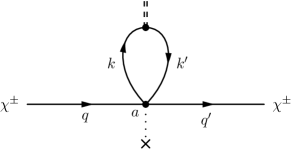
Figure 4: One-loop local $\chi$ self-energy: $i\Pi^{\mathrm{loc}(1)}_{\chi,\,ab}(q,q^{\prime},\tilde{t}_{f};\tilde{t}_{i})\>\propto\>\eta_{ab}$.

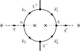
(a) $i\Pi^{(1)}_{\Phi,\,ab}(q,q^{\prime},\tilde{t}_{f};\tilde{t}_{i})$

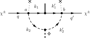
(b) $i\Pi^{(1)}_{\chi,\,ab}(q,q^{\prime},\tilde{t}_{f};\tilde{t}_{i})$

Figure 5: Non-local one-loop $\Phi$ (a) and $\chi$ (b) self-energies.

IX.1 Time-Dependent Width

In this section, we study the time-dependent width of the heavy scalar $\Phi$. In particular, we investigate the spectral evolution that results from the restoration of energy conservation, without solving explicitly the system of evolution equations for the statistical dynamics.

We consider the following situation. We prepare two isolated but coincident subsystems $\mathscr{S}_{\Phi}$ and $\mathscr{S}_{\chi}$, both separately in thermodynamic equilibrium and at the same temperature $T$, with all interactions turned off. The subsystem $\mathscr{S}_{\Phi}$ contains only the real scalar field $\Phi$, whilst $\mathscr{S}_{\chi}$ contains only the complex scalar $\chi$. At macroscopic time $t\>=\>0$, we turn on the interactions and allow the system $\mathscr{S}\>=\>\mathscr{S}_{\Phi}\>\cup\>\mathscr{S}_{\chi}$ to re-thermalize. For our numerical analysis, we take for definiteness the thermodynamic temperature to be $T\>=\>10\ \mathrm{GeV}$, the mass of the heavy $\Phi$-scalar $M\>=\>1\ \mathrm{GeV}$, the mass of the complex $\chi$-scalar $m\>=\>0.01\ \mathrm{GeV}$, and their trilinear coupling $g\>=\>0.1\ \mathrm{GeV}$.

The free propagators of the fields $\Phi$ and $\chi$ at time $t\>=\>0$ are the equilibrium propagators in (171) and (370), containing the Bose–Einstein distributions at temperature $T$. We take the chemical potential of the complex scalar to be vanishingly small in comparison to the temperature, i.e. $\mu/T\>\ll\>1$, such that $f_{\chi}(|\mathbf{p}|,0)\>=\>f^{C}_{\chi}(|\mathbf{p}|,0)\>=\>f_{\mathrm{B}}\big{(}E_{\chi}(\mathbf{p})\big{)}$. Without solving the system of time evolution equations, the form of the the statistical distribution functions of the $\Phi$ and $\chi$ scalars is unknown for $t\>\neq\>0$. We assume that the heat bath of $\chi$’s is sufficiently large so as to remain unperturbed by the addition of the real scalar $\Phi$. Specifically, we may consider the number density of $\chi$’s to remain unchanged and the free equilibrium $\chi$ propagators in (370) to persist for all times.

By the optical theorem, the width $\Gamma_{\Phi}$ of the scalar $\Phi$ is defined in terms of the absorptive part of the retarded $\Phi$ self-energy $\mathrm{Im}\,\Pi_{\Phi,\,\mathrm{R}}$ via

$$\Gamma_{\Phi}(q_{1},q_{2},\tilde{t}_{f};\tilde{t}_{i})\ =\ \frac{1}{M}\mathrm{Im}\,\Pi_{\Phi,\,\mathrm{R}}(q_{1},q_{2},\tilde{t}_{f};\tilde{t}_{i})\;,$$ (266)

where

$$\mathrm{Im}\,\Pi_{\Phi,\,\mathrm{R}}(q_{1},q_{2},\tilde{t}_{f};\tilde{t}_{i})\ =\ \frac{1}{2i}\Big{(}\,\Pi_{\Phi,\,>}(q_{1},q_{2},\tilde{t}_{f};\tilde{t}_{i})\>-\>\Pi_{\Phi,\,<}(q_{1},q_{2},\tilde{t}_{f};\tilde{t}_{i})\,\Big{)}\;.$$ (267)

At the one-loop level, the self-energies $\Pi^{(1)}_{\Phi,\,\gtrless}(q_{1},q_{2},\tilde{t}_{f};\tilde{t}_{i})$ are given by (265).

Employing the relative and central momenta, $Q\>=\>q_{1}\>-\>q_{2}$ and $q\>=\>(q_{1}\>+\>q_{2})/2$, and using the results of Appendix F, the Laplace transform with respect to the macroscopic time $t$ of the one-loop $\Phi$ width is

$$\Gamma^{(1)}_{\Phi}(q+Q/2,q-Q/2,s)\ =\ (2\pi)^{4}\frac{1}{\pi}\,\frac{s}{Q_{0}^{2}\>+\>4s^{2}}e^{iQ_{0}\tilde{t}_{f}}\delta^{(3)}(\mathbf{Q})$$

$$\hskip 85.35826pt\times\ \frac{g^{2}}{32\pi^{2}M}\sum_{\{\alpha\}}\int\!\mathrm{d}^{3}{\mathbf{k}}\;\frac{1}{\pi}\,\frac{\alpha_{1}\alpha_{2}}{E_{1}E_{2}}\,\frac{1\>+\>f_{\mathrm{B}}\big{(}\alpha_{1}E_{1}\big{)}\>+\>f_{\mathrm{B}}\big{(}\alpha_{2}E_{2}\big{)}}{\big{(}q_{0}^{2}\>-\>\alpha_{1}E_{1}\>-\>\alpha_{2}E_{2}\big{)}^{2}\>+\>s^{2}}\;,$$ (268)

where we use the short-hand notation $\{\alpha\}$ for the summation over $\alpha_{1},\ \alpha_{2}\>=\>\pm 1$. For the sake of generality, we distinguish the $\chi^{+}$ and $\chi^{-}$ decay products by assigning them different masses $m_{1}$ and $m_{2}$, respectively, so that

$$E_{1}\ \equiv\ E_{1}(\mathbf{k})\ =\ \sqrt{|\mathbf{k}|^{2}\>+\>m_{1}^{2}}\;,$$ (269a)

$$E_{2}\ \equiv\ E_{2}(\mathbf{q}-\mathbf{k})\ =\ \sqrt{|\mathbf{k}|^{2}\>-\>2|\mathbf{k}||\mathbf{q}|\cos\theta\>+\>|\mathbf{q}|^{2}\>+\>m_{2}^{2}}\;.$$ (269b)

In our numerical analysis, however, we take $m_{1}\>=\>m_{2}\>=\>m$.

Performing the inverse Wigner transform with respect to $Q$ of (IX.1) in the equal-time limit $X_{0}\>=\>\tilde{t}_{f}$ and subsequently the inverse Laplace transform with respect to $s$, we obtain the time-dependent $\Phi$ width

$$\Gamma^{(1)}_{\Phi}(q,t)\ =\ \frac{g^{2}}{64\pi^{2}M}\sum_{\{\alpha\}}\int\!\mathrm{d}^{3}{\mathbf{k}}\;\frac{\alpha_{1}\alpha_{2}}{E_{1}E_{2}}\,\frac{t}{\pi}\,\mathrm{sinc}\big{[}\big{(}q_{0}\>-\>\alpha_{1}E_{1}\>-\>\alpha_{2}E_{2}\big{)}t\big{]}\Big{(}\,1\>+\>f_{\mathrm{B}}\big{(}\alpha_{1}E_{1}\big{)}\>+\>f_{\mathrm{B}}\big{(}\alpha_{2}E_{2}\big{)}\,\Big{)}\;.$$ (270)

In the limit $t\>\to\>\infty$, the sinc function on the RHS of (270) yields the standard energy-conserving delta function:

$$\lim_{t\>\to\>\infty}\,\frac{t}{\pi}\,\mathrm{sinc}\big{[}\big{(}q_{0}\>-\>\alpha_{1}E_{1}\>-\>\alpha_{2}E_{2}\big{)}t\big{]}\ =\ \delta\big{(}q_{0}\>-\>\alpha_{1}E_{1}\>-\>\alpha_{2}E_{2}\big{)}\;,$$ (271)

thereby recovering the known equilibrium result.

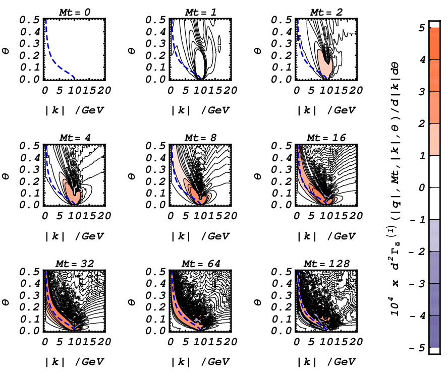
Figure 6: Contour plots of $|\mathbf{k}|$ versus $\theta$ for $\mathrm{d}^{2}{\Gamma_{\Phi}^{(1)}}$ for discrete values of $Mt$, with $q^{2}\>=\>M^{2}$ and $|\mathbf{q}|\>=\>10\,\mathrm{GeV}$. The region of phase space permitted in the $t\>\to\>\infty$ limit is shown by the blue dashed line, corresponding to the delta function in (271).

Figure 6 contains a series of contour plots of the differential one-loop $\Phi$ width $\mathrm{d}^{2}{\Gamma^{(1)}_{\Phi}}$ evaluated over the dominant region of the $|\mathbf{k}|$-$\theta$ phase space, where the four-momentum $q^{\mu}$ of the $\Phi$ scalar is on-shell, i.e. $q^{2}=M^{2}$. For late times, the integrand is highly oscillatory and we expect the dominant peak of the sinc function to approach the region of phase space permitted in the limit $t\>\to\>\infty$ [cf. (271)], for which

$$|\mathbf{k}|\ =\ \frac{M^{2}|\mathbf{q}|\cos\theta\>+\>\sqrt{\big{(}|\mathbf{q}|^{2}\>+\>M^{2}\big{)}\big{[}M^{4}\>-\>4m^{2}\big{(}M^{2}\>+\>|\mathbf{q}|^{2}\sin^{2}\!\theta\big{)}\big{]}}}{2\big{(}M^{2}\>+\>|\mathbf{q}|^{2}\sin^{2}\!\theta\big{)}}\;.$$ (272)

For early times, the admissible phase space is greatly expanded. For later times, the frequency of oscillation increases and the width of the central peak of the sinc function narrows, lying along a curve in the phase space. To proceed further, we need to develop a method for dealing with the kinematics in the absence of exact energy conservation.

IX.2 Generalized Two-Body Decay Kinematics

At zero temperature and density, it is convenient to analyze the two-body decay kinematics by performing a Lorentz boost to the rest frame of the decaying particle. However, at finite temperature, the dependence on the thermodynamic temperature of the heat bath breaks the Lorentz covariance of the integral. As such, we cannot eliminate dependence upon the the three-momentum of the decaying particle by any such Lorentz boost; the dependence will reappear in the ‘boosted’ temperature:

$$T^{\prime}\ =\ \gamma\,T\;,$$ (273)

where

$$\gamma\ =\ \Bigg{(}1\>+\>\frac{|\mathbf{q}|^{2}}{M^{2}}\Bigg{)}^{1/2}$$ (274)

is the usual Lorentz boost factor for the heavy scalar field $\Phi$. As a result, we are compelled to analyze the kinematics of the two-body decay in the rest frame of the heat bath, which we define to be the frame in which the EEV of the three-momentum operator $\braket{\widehat{\bf P}}$ is minimized. For an isotropic heat bath, this is the frame in which $\braket{\widehat{\bf P}}\>=\>\mathbf{0}$, that is the comoving frame. In this section, we look more closely at the kinematics in the absence of energy conservation.

For this purpose, let us introduce the variable

$$u\ \equiv\ \big{(}q_{0}\>-\>\alpha_{1}E_{1}\>-\>\alpha_{2}E_{2}\big{)}t\;,$$ (275)

which may be interpreted in terms of energy borrowed from or lent to the heat bath. We shall hereafter refer to the variable $u$ as the evanescent action of the process, since it has the correct dimensions and quantifies the extended kinematically allowed phase-space configurations. We also define the evanescent energy

$$q_{u}(t)\ \equiv\ q_{0}\>-\>\frac{u}{t}\;,$$ (276)

which satisfies

$$\lim_{u/t\>\to\>0}\,q_{u}(t)\ =\ q_{0}\;.$$ (277)

With this substitution, we obtain the kinematic constraint

$$q_{u}(t)\>-\>\alpha_{1}E_{1}\>-\>\alpha_{2}E_{2}\ =\ 0\;.$$ (278)

Since $u$ can take large positive values, $q_{u}(t)$ is not necessarily restricted to positive values for early times, even when $q_{0}\>=\>\sqrt{|\mathbf{q}|^{2}\>+\>M^{2}}\>>\>0$ is on-shell. Processes with $u/t\>\neq\>0$ are referred to as evanescent.

In order to make the coordinate transformation $|\mathbf{k}|\>\to\>u$ in (270), we must solve (278) for the magnitude of the three-momentum $|\mathbf{k}(t)|$, which becomes implicitly time dependent. Specifically, we find

$$|\mathbf{k}^{(b)}(t)|\ =\ \frac{1}{2\big{(}q_{u}^{2}(t)\>-\>|\mathbf{q}|^{2}\cos^{2}\!\theta\big{)}}\Big{[}\,\big{(}q_{u}^{2}(t)\>-\>|\mathbf{q}|^{2}\>+\>m_{1}^{2}\>-\>m_{2}^{2}\big{)}|\mathbf{q}|\cos\theta$$

$$\qquad+\>b\,q_{u}(t)\sqrt{\lambda\big{(}q_{u}^{2}(t)\>-\>|\mathbf{q}|^{2},m_{1}^{2},m_{2}^{2}\big{)}\>-\>4m_{1}^{2}|\mathbf{q}|^{2}\sin^{2}\!\theta}\;\Big{]}\;,$$ (279)

with $b\>=\>\pm 1$ and

$$\lambda(x,y,z)\ =\ (x-y-z)^{2}\>-\>4yz\;.$$ (280)

After a little algebra, we obtain the energies

$$E_{1}^{(b)}(t)\ =\ \alpha_{1}\frac{1}{2\big{(}q_{u}^{2}(t)\>-\>|\mathbf{q}|^{2}\cos^{2}\!\theta\big{)}}\Big{[}\,\big{(}q_{u}^{2}(t)\>-\>|\mathbf{q}|^{2}\>+\>m_{1}^{2}\>-\>m_{2}^{2}\big{)}q_{u}(t)$$

$$\qquad+\>b\,|\mathbf{q}|\cos\theta\sqrt{\lambda\big{(}q_{u}^{2}(t)\>-\>|\mathbf{q}|^{2},m_{1}^{2},m_{2}^{2}\big{)}\>-\>4m_{1}^{2}|\mathbf{q}|^{2}\sin^{2}\!\theta}\;\Big{]}\;,$$ (281)

$$E_{2}^{(b)}(t)\ =\ \alpha_{2}\frac{1}{2\big{(}q_{u}^{2}(t)\>-\>|\mathbf{q}|^{2}\cos^{2}\!\theta\big{)}}\Big{[}\,\big{(}q_{u}^{2}(t)\>-\>|\mathbf{q}|^{2}\cos 2\theta\>-\>m_{1}^{2}\>+\>m_{2}^{2}\big{)}q_{u}(t)$$

$$\qquad-\>b\,|\mathbf{q}|\cos\theta\sqrt{\lambda\big{(}q_{u}^{2}(t)\>-\>|\mathbf{q}|^{2},m_{1}^{2},m_{2}^{2}\big{)}\>-\>4m_{1}^{2}|\mathbf{q}|^{2}\sin^{2}\!\theta}\;\Big{]}\;,$$ (282)

where the overall factors of $\alpha_{1}$ and $\alpha_{2}$ are necessary to satisfy the initial constraint (278). It is clear that these results collapse to the kinematics of equilibrium field theory in the limit $u/t\>\to\>0$.

Keeping $m_{1}$ and $m_{2}$ distinct, the $\Phi$ width for $t\>>\>0$ is given by

$$\Gamma^{(1)}_{\Phi}(q,t)\ =\ \frac{g^{2}}{64\pi^{2}M}\sum_{\{\alpha\},\,b\>=\>\pm 1}\int_{0}^{\pi}\!\mathrm{d}{\theta}\int_{u_{-}(t)}^{u_{+}(t)}\!\!\mathrm{d}{u}\,\,\mathrm{sinc}(u)\,\frac{\sin\theta}{\big{(}q_{u}^{2}(t)\>-\>|\mathbf{q}|^{2}\cos^{2}\!\theta\big{)}^{2}}$$

$$\qquad\times\>\Big{[}\,\lambda\big{(}q_{u}^{2}(t)\>-\>|\mathbf{q}|^{2},m_{1}^{2},m_{2}^{2}\big{)}\>-\>4m_{1}^{2}|\mathbf{q}|^{2}\sin^{2}\!\theta\,\Big{]}^{-1/2}$$

$$\qquad\times\>\Big{[}\,\big{(}q_{u}^{2}(t)\>-\>|\mathbf{q}|^{2}\>+\>m_{1}^{2}\>-\>m_{2}^{2}\big{)}|\mathbf{q}|\cos\theta\>+\>b\,q_{u}(t)\sqrt{\lambda\big{(}q_{u}^{2}(t)\>-\>|\mathbf{q}|^{2},m_{1}^{2},m_{2}^{2}\big{)}\>-\>4m_{1}^{2}|\mathbf{q}|^{2}\sin^{2}\!\theta}\,\Big{]}^{2}$$

$$\qquad\times\>\alpha_{1}\alpha_{2}\Big{(}\,1\>+\>f_{\mathrm{B}}\big{(}\alpha_{1}E^{(b)}_{1}(t)\big{)}\>+\>f_{\mathrm{B}}\big{(}\alpha_{2}E^{(b)}_{2}(t)\big{)}\,\Big{)}\;.$$ (283)

The reality of the loop momentum $|\mathbf{k}(t)|$ in (IX.2) requires that the discriminant

$$\lambda\big{(}q_{u}^{2}(t)\>-\>|\mathbf{q}|^{2},m_{1}^{2},m_{2}^{2}\big{)}\>-\>4m_{1}^{2}|\mathbf{q}|^{2}\sin^{2}\!\theta\ \geq\ 0\;,$$ (284)

which is now a time-dependent kinematic constraint. Furthermore, we require $|\mathbf{k}^{(b)}(t)|\>\geq\>0$, $E^{(b)}_{1}(t)\>\geq\>m_{1}$ and $E^{(b)}_{2}(t)\>\geq\>m_{2}$. For $t\>>\>0$, the limits of integration $u_{\pm}(t)$ are given in Table 3, where we have defined

$$\omega_{0}(q,\alpha_{1},\alpha_{2})\ \equiv\ q_{0}\>-\>\big{(}\alpha_{1}m_{1}\>+\>\alpha_{2}m_{2}\big{)}\Bigg{(}1\>+\>\dfrac{|\mathbf{q}|^{2}}{\big{(}m_{1}\>+\>m_{2}\big{)}^{2}}\Bigg{)}^{\!\!1/2}\;,$$ (285)

which is the angular frequency of the sine-integral-like oscillations of the integral. For $t\>=\>0$, $u_{\pm}(t)\>=\>0$ and the domain of integration over $u$ collapses to zero. Given the analytic behavior of the integrand in the limit $t\>\to\>0$, the integral vanishes, as we expect.

Table 3: Limits of integration of the evanescent action $u$ for each of the four processes contributing to the non-equilibrium thermal $\Phi$ width of our specific model for $t\>>\>0$, where the angular frequency $\omega_{0}(q,\alpha_{1},\alpha_{2})$ is defined in (285).

	$\alpha_{1}\ =\ \alpha_{2}\ =\ +1$	$\alpha_{1}\ =\ -\alpha_{2}$	$\alpha_{1}\ =\ \alpha_{2}\ =\ -1$
$u_{+}(t)$	$\omega_{0}(q,\alpha_{1},\alpha_{2})t$	$\omega_{0}(q,\alpha_{1},\alpha_{2})t$	$+\infty$
$u_{-}(t)$	$-\infty$	$0$	$\omega_{0}(q,\alpha_{1},\alpha_{2})t$

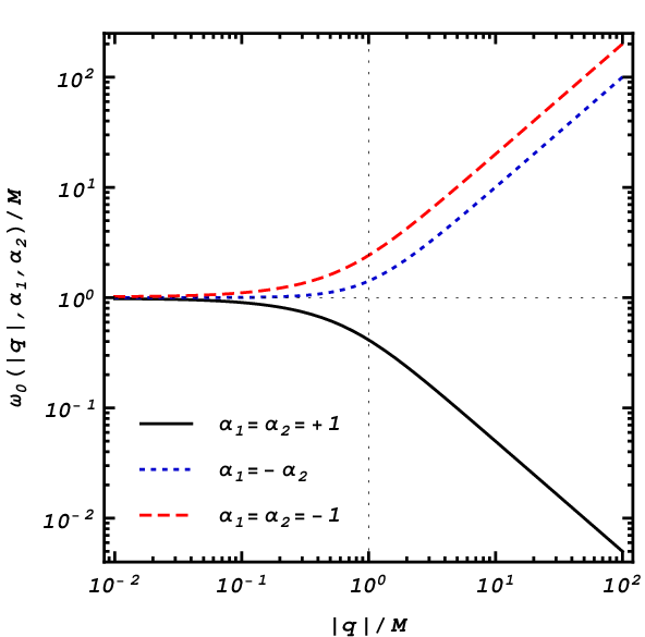
Figure 7: The dependence of $\omega_{0}(|\mathbf{q}|,\alpha_{1},\alpha_{2})/M$ on $|\mathbf{q}|/M$ for processes related to $1\>\to\>2$ decay (solid black), Landau damping (blue dotted) and $3\>\to\>0$ total annihilation (red dashed), where $q^{2}\>=\>M^{2}$ and $m_{1}\>=\>m_{2}\>=\>m\>=0.01\,\mathrm{GeV}$. The latter two of these processes become highly oscillatory for large $|\mathbf{q}|/M$.

For on-shell decay modes with $q^{2}\>=\>M^{2}$, the angular frequency $\omega_{0}(q,1,1)$ in (285) becomes

$$\omega_{0}(|\mathbf{q}|,1,1)\ \equiv\ \omega_{0}(q,1,1)\big{|}_{q^{2}\>=\>M^{2}}\ =\ \sqrt{|\mathbf{q}|^{2}\>+\>M^{2}}\>-\>\sqrt{|\mathbf{q}|^{2}\>+\>\big{(}m_{1}\>+\>m_{2}\big{)}^{2}}\;.$$ (286)

Thus, the evolution of the phase space for on-threshold decays with $M^{2}\>=\>(m_{1}\>+\>m_{2})^{2}$ is critically damped. We note that in the large momentum limit $|\mathbf{q}|\>\gg\>M$,

$$\omega_{0}(|\mathbf{q}|,1,1)\big{|}_{|\mathbf{q}|\>\gg\>M}\ \simeq\ \frac{M^{2}\>-\>\big{(}m_{1}\>+\>m_{2}\big{)}^{2}}{2|\mathbf{q}|}\;,$$ (287)

such that the evolution of the phase space for high-momentum modes is similarly damped. The momentum dependence of $\omega_{0}(|\mathbf{q}|,\alpha_{1},\alpha_{2})$ is shown in Figure 7.

(a) $1\rightarrow 2$ decay

(b) $2\rightarrow 1$ Landau damping

(c) $3\rightarrow 0$ total annihilation

Figure 8: Processes contributing to the time-dependent $\Phi$ width: (a) the familiar $1\>\rightarrow\>2$ decay; (b) $2\>\rightarrow\>1$ Landau damping; and (c) $3\>\rightarrow\>0$ total annihilation.

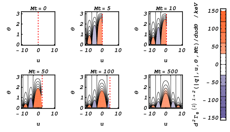
Figure 9: Contour plots of $u$ versus $\theta$ for the $1\>\rightarrow\>2$ decay contribution to $\mathrm{d}^{2}{\Gamma_{\Phi}^{(1)}}$ for discrete values of $Mt$, with $q^{2}\>=\>M^{2}$ and $|\mathbf{q}|\>=\>10\ \mathrm{GeV}$. The solid excluded regions to the right of the red dotted line lie exterior to the limits of integration over $u$.

The summation over $\alpha_{1}$ and $\alpha_{2}$ yields four distinct contributions to the decay width Berges (2004, 2005). For $\alpha_{1}\>=\>\alpha_{2}\>=\>+1$, we obtain the contribution from the familiar $1\>\rightarrow\>2$ decay process presented in Figure 8a. For $\alpha_{1}\>=\>-\alpha_{2}\>=\>\pm 1$, we obtain the two $2\>\rightarrow\>1$ Landau–damping contributions displayed in Figure 8b. For $\alpha_{1}\>=\>\alpha_{2}\>=\>-1$, we obtain the $3\>\rightarrow\>0$ total annihilation process shown in Figure 8c. In the latter, the decay ‘products’ appear in the initial state along with the decaying particle. For late times, the Landau–damping and total annihilation processes are kinematically disallowed, as we would expect. They are only permitted in the evanescent regime at early times.

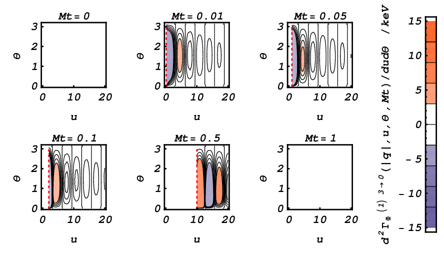
Figure 10: Contour plots of $u$ versus $\theta$ for the $3\>\rightarrow\>0$ total annihilation contribution to $\mathrm{d}^{2}{\Gamma_{\Phi}^{(1)}}$ for discrete values of $Mt$, where $q^{2}\>=\>M^{2}$ and $|\mathbf{q}|\>=\>10\ \mathrm{GeV}$. The regions to the left of the red dotted line are exterior to the domain of integration over $u$.

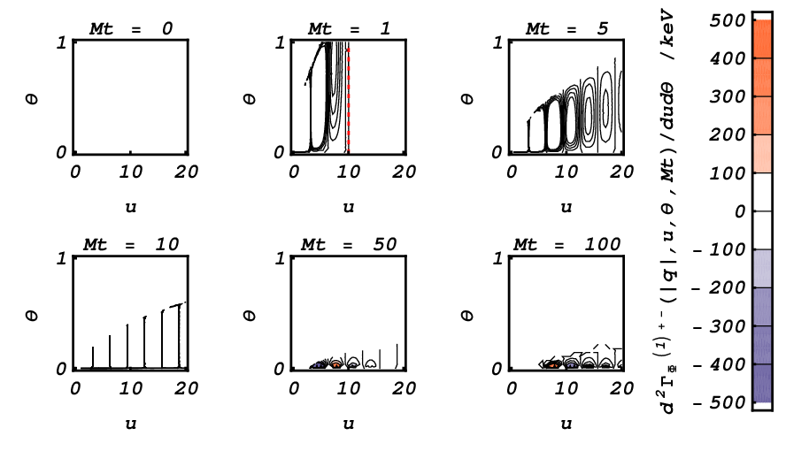
(a) $\alpha_{1}\ =\ -\alpha_{2}\ =\ +1$

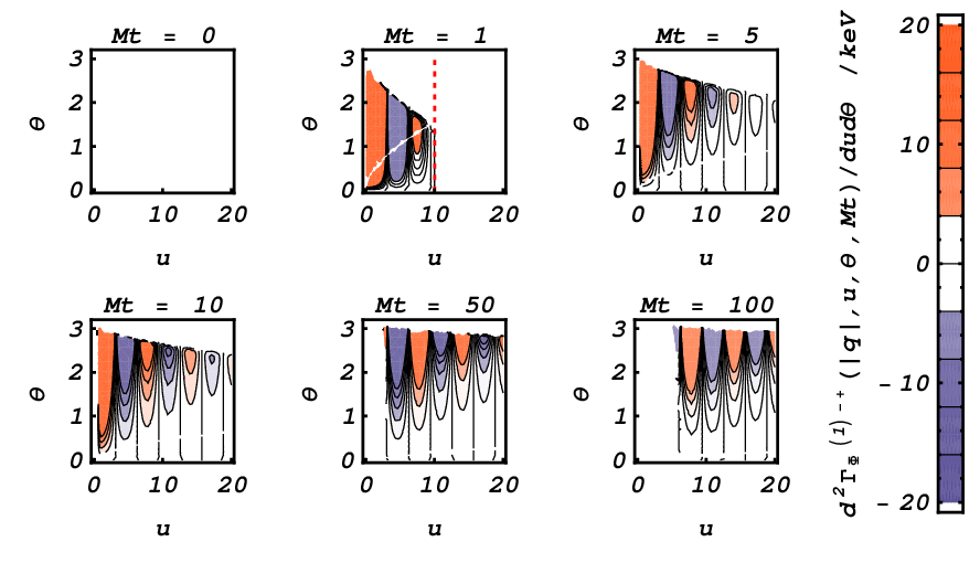
(b) $\alpha_{1}\ =\ -\alpha_{2}\ =\ -1$

Figure 11: Contour plots of $u$ versus $\theta$ for the two Landau–damping contributions (a) ${\alpha_{1}\>=\>-\alpha_{2}\>=\>+1}$ and (b) $\alpha_{1}\>=\>-\alpha_{2}\>=\>-1$ to $\mathrm{d}^{2}{\Gamma_{\Phi}^{(1)}}$ for discrete values of $Mt$, assuming $q^{2}\>=\>M^{2}$ and ${|\mathbf{q}|\>=\>10\ \mathrm{GeV}}$. The regions to the right of the red dotted line are exterior to the domain of integration over $u$. The contour plots differ between the two contributions due to the asymmetry of the integrands in the $\Phi$ three-momentum.

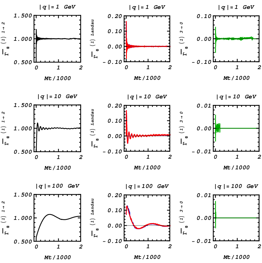
Figure 12: The four separate contributions to the ratio $\bar{\Gamma}_{\Phi}^{(1)}$ in (292) versus $Mt$, for on-shell decays with $|\mathbf{q}|\>=\>1\ \mathrm{GeV}$, $10\ \mathrm{GeV}$ and $100\ \mathrm{GeV}$. The two Landau–damping contributions are identical up to numerical errors.

Figures 9–11 contain contour plots of $u$ versus $\theta$ for the four contributions to the on-shell differential width $\mathrm{d}^{2}{\Gamma_{\Phi}^{(1)}}$. The equilibrium kinematics are obtained in the large-time limit $t\>\to\>\infty$ as follows. As can be seen from the $(u,\theta)$ contour plots in Figure 9, for the $1\>\to\>2$ decay process, the limits of integration grow to encompass the full range of the sinc function. At the same time, the $u$ dependence of the phase-space pre-factors vanishes, since $q_{u}(t)\>\to\>q_{0}$ as $t\>\to\>\infty$. For the $3\>\to\>0$ total annihilation process, the domain of integration vanishes in the large-time limit $t\>\to\>\infty$. Given that the integrand is finite in the same limit, the contribution therefore vanishes as expected, which is confirmed by our $(u,\theta)$ contour plots in Figure 10. For the two Landau–damping contributions, the large-time behavior becomes more subtle. As $t\>\to\>\infty$, the domain of integration covers approximately all positive $u$. However, the kinematically allowed phase space cannot be attained with any values of $u$ and $\theta$, so that the two Landau–damping contributions also vanish in the large-time limit. This behavior is reflected in our $(u,\theta)$ contour plots of Figure 11. Thus, only the usual $1\>\to\>2$ energy-conserving decay remains for late times.

In order to reduce the statistical error in our Monte Carlo integration over the $(u,\theta)$ phase space, we use a Gaussian sampling bias to ensure that the majority of sampling points fall over the dominant region of the sinc function of $u$ in (IX.2). We define the weight function

$$\varpi(u)\ =\ \frac{\mathrm{d}{u}}{\mathrm{d}{r}}\ \equiv\ \exp\bigg{(}-\frac{(u\>-\>u_{0})^{2}}{2\sigma_{u}^{2}}\bigg{)}$$ (288)

where

$$r(u)\ \equiv\ \frac{\mathrm{Erf}\Big{(}\frac{1}{\sqrt{2}}\,\frac{u\>-\>u_{0}}{\sigma_{u}}\Big{)}\>-\>\mathrm{Erf}\Big{(}\frac{1}{\sqrt{2}}\,\frac{u_{-}\>-\>u_{0}}{\sigma_{u}}\Big{)}}{\mathrm{Erf}\Big{(}\frac{1}{\sqrt{2}}\,\frac{u_{+}\>-\>u_{0}}{\sigma_{u}}\Big{)}\>-\>\mathrm{Erf}\Big{(}\frac{1}{\sqrt{2}}\,\frac{u_{-}\>-\>u_{0}}{\sigma_{u}}\Big{)}}\ \in\ [0,\ 1]\;.$$ (289)

After performing the change of the variable $u\>\to\>r$ in (IX.2) for $u_{0}\>=\>0$, the limits of integration become time-independent and are identical for the decay, total-annihilation and Landau–damping contributions. The dependence upon the limits $u_{+}(t)$ and $u_{-}(t)$ appears instead within the transformed integrand of (IX.2) in the new variables $(r,\theta)$.

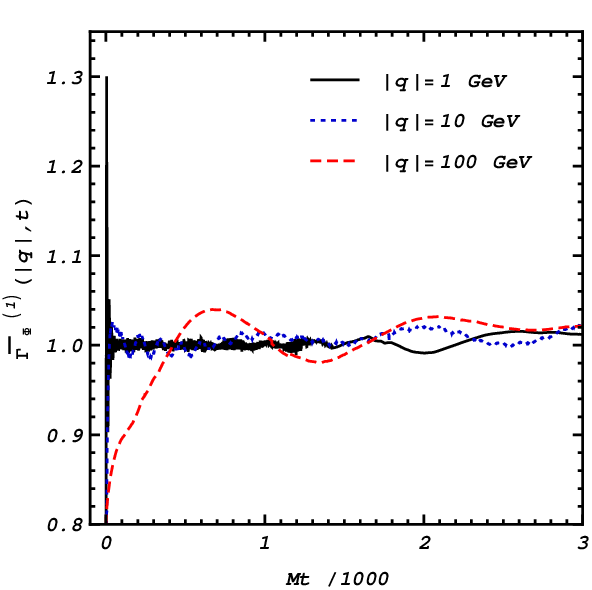
Figure 13: The ratio $\bar{\Gamma}_{\Phi}^{(1)}$ in (292) versus $Mt$, for on-shell decays with $|\mathbf{q}|\>=\>1\ \mathrm{GeV}$ (solid black), $10\ \mathrm{GeV}$ (blue dotted) and $100\ \mathrm{GeV}$ (red dashed).

The width of the dominant region of the $u$ phase-space is taken to be the distance between the central maximum and the maximum at which the amplitude of the sinc function has fallen to $0.1\%$ with respect to the central maximum. Hence, we require for the distant maximum to be at the location where $\mathrm{sinc}\,u_{n}\>\sim\>0.001$. The extrema $u_{n}$ of the sinc function satisfy the transcendental equation

$$u_{n}\ =\ \tan u_{n}\;,$$ (290)

whose solutions for $n\>\geq\>1$ may be expressed as Burniston and Siewert (1973)

$$u_{n}\ =\ \pm n\pi\exp\bigg{\{}\frac{1}{\pi}\!\int_{0}^{1}\!\mathrm{d}{\xi}\;\frac{1}{\xi}\,\mathrm{arg}\bigg{[}\bigg{(}1\>+\>\frac{1}{2}\xi\ln\frac{1\>-\;\xi}{1\>+\>\xi}\>\pm\>\frac{1}{2}\pi i\xi\bigg{)}^{\!\!2}\!\>+\>n^{2}\pi^{2}\xi^{2}\,\bigg{]}\bigg{\}}\;.$$ (291)

The required extremum is then given by $n\>=\>318$, the 159^th maximum of the sinc function, with $u_{318}\>=\>1000$. The Gaussian weight function $\varpi(u)$ in (288) is then taken to have a variance of $\sigma_{u}^{2}\>=\>(u_{318}/2)^{2}$, such that $95\%$ of the sampling points fall within this dominant region.

Our interest is in the deviation of the one-loop $\Phi$ width $\Gamma_{\Phi}^{(1)}$ from the known equilibrium result. It is therefore convenient to define the ratio $\bar{\Gamma}_{\Phi}^{(1)}(|\mathbf{q}|,t)$ of the time-dependent width to its late-time equilibrium value for $q^{2}\>=\>M^{2}$:

$$\bar{\Gamma}_{\Phi}^{(1)}(|\mathbf{q}|,t)\ =\ \frac{\Gamma_{\Phi}^{(1)}(|\mathbf{q}|,t)}{\Gamma_{\Phi}^{(1)}(|\mathbf{q}|,t\>\to\>\infty)}\ =\ \frac{\Gamma_{\Phi}^{(1)1\rightarrow 2}(|\mathbf{q}|,t)\>+\>2\Gamma_{\Phi}^{(1)\mathrm{Landau}}(|\mathbf{q}|,t)\>+\>\Gamma_{\Phi}^{(1)3\rightarrow 0}(|\mathbf{q}|,t)}{\Gamma_{\Phi}^{(1)}(|\mathbf{q}|,t\to\infty)}\;.$$ (292)

In Figure 12, we plot separately the four contributions from Figure 8 to this ratio as a function of $Mt$ for a series of discrete momenta. The evanescent Landau–damping processes yield a prompt contribution, which can be as high as $10$–$20\%$ at early times. The evanescent total annihilation process contributes similarly at the level of about $5\%$.

In Figure 13, we plot the total ratio $\bar{\Gamma}_{\Phi}^{(1)}(|\mathbf{q}|,t)$ as a function of $Mt$. The total $\Phi$ width $\Gamma^{(1)}_{\Phi}(|\mathbf{q}|,t)$ is vanishing for ${Mt\>=\>0}$, as we would expect. This is followed promptly by a sharp rise, which is particularly pronounced in the infra-red modes, resulting from the sudden switching on of the interactions. This so-called shock regime is followed by the superposition of transient oscillations of angular frequency $\omega_{0}$ with short time scales and non-Markovian oscillations of longer time scales. The latter of these oscillations exhibit time-dependent frequencies, the origin of which will be discussed in the next section.

IX.3 Non-Markovian Oscillations

As we have seen in Figures 12 and 13, the time-dependent $\Phi$ width contains a superposition of damped oscillatory contributions. The longer lived of these oscillations exhibit time-dependent frequencies. These non-Markovian oscillations are illustrated more clearly in Figure 14 for the $|\mathbf{q}|\>=\>1\ \mathrm{GeV}$ mode in which a moving time average is carried out to eliminate the higher-frequency Markovian oscillations. In this section, we describe the origin of the time-dependent oscillations and show that they are not a numerical artefact, but are instead an intrinsic feature inherent to the dynamics of truly out-of-equilibrium systems. To this end, we consider the high-temperature limit $T\>\gg\>M$ of the time-dependent $\Phi$ width.

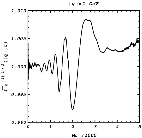
Figure 14: Non-Markovian oscillations of the $1\>\to\>2$ decay contribution to the ratio $\bar{\Gamma}_{\Phi}^{(1)}$ in (292) against $Mt$, by performing a moving average over bins of $150$ in $Mt$.

In this high-temperature limit $T\>\gg\>M$, the Bose–Einstein distribution may be approximated as follows:

$$f_{\mathrm{B}}(E)\ \approx\ \frac{T}{E}\;,$$ (293)

Returning to the $\Phi$ width $\Gamma^{(1)}_{\Phi}$ in (270) and substituting for (293), we may perform the angular integration by making the following change of variables:

$$\cos\theta\ =\ \frac{|\mathbf{k}|^{2}\>+\>|\mathbf{q}|^{2}\>+\>m_{2}^{2}}{2|\mathbf{k}||\mathbf{q}|}\,(1\>-\>x^{2})\;.$$ (294)

Then, the high-temperature limit $T\>\gg\>M$ of the time-dependent width of the heavy scalar $\Phi$ becomes

$$\Gamma^{(1),\,T\>\gg\>M}_{\Phi}(q,t)\ =\ \frac{g^{2}}{32\pi^{2}M}\sum_{\{\alpha\}}\alpha_{1}\alpha_{\theta}\!\int_{0}^{\infty}\!\!\mathrm{d}{|\mathbf{k}|}\;\frac{|\mathbf{k}|}{|\mathbf{q}|}\,\frac{1}{E_{1}}$$

$$\quad\quad\times\ \Bigg{[}\Bigg{(}1\>+\>\frac{T}{\alpha_{1}E_{1}}\>+\>\frac{T}{q_{0}\>-\>\alpha_{1}E_{1}}\Bigg{)}\mathrm{Si}\big{[}\big{(}q_{0}\>-\>\alpha_{1}E_{1}\>-\>\alpha_{2}E_{2}\big{)}t\big{]}$$

$$\quad\quad-\ \frac{T}{q_{0}\>-\>\alpha_{1}E_{1}}\Bigg{(}\sin\!\big{[}\big{(}q_{0}\>-\>\alpha_{1}E_{1}\big{)}t\big{]}\mathrm{Ci}\big{(}\alpha_{2}E_{2}t\big{)}\>-\>\cos\!\big{[}\big{(}q_{0}\>-\>\alpha_{1}E_{1}\big{)}t\big{]}\mathrm{Si}\big{(}\alpha_{2}E_{2}t\big{)}\Bigg{)}\Bigg{]}\;,$$ (295)

where $\mathrm{Si}(x)$ and $\mathrm{Ci}(x)$ are respectively the sine integral and cosine integral functions. We have introduced the short-hand notations: $\{\alpha\}$ for the summation over $\alpha_{1},\ \alpha_{2},\ \alpha_{\theta}\>=\>\pm 1$; and

$$E_{1} \ =\ \sqrt{|\mathbf{k}|^{2}\>+\>m_{1}^{2}}\>,$$ (296)

$$E_{2} \ =\ \sqrt{|\mathbf{k}|^{2}\>-\>2\alpha_{\theta}|\mathbf{k}||\mathbf{q}|\>+\>|\mathbf{q}|^{2}\>+\>m_{2}^{2}}\;.$$ (297)

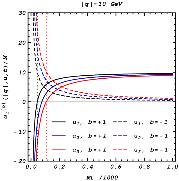
Figure 15: $\omega^{(b)}_{1}(q,u,t)/M$ versus $Mt$ for the first three extrema of $\mathrm{sinc}(u)$: $u_{1}\>=\>4.49$ (left-most black lines), $u_{2}\>=\>7.73$ (central blue lines) and $u_{3}\>=\>10.90$ (right-most red lines), obtained by (291), for $q^{2}\>=\>M^{2}$, $|\mathbf{q}|\>=\>10\ \mathrm{GeV}$ and $\alpha_{\theta}\>=\>+1$. Solid lines correspond to $b\>=\>1$ and dashed lines, $b\>=\>-1$ in (299a). The dotted lines mark the upper limit of the kinematically disallowed region.

In terms of the evanescent action $u$ given in (275), the high-temperature limit of the one-loop $\Phi$ width reads:

$$\Gamma_{\Phi}^{(1),\,T\>\gg\>M}(q,t)\ =\ \frac{g^{2}}{32\pi^{2}Mt}\sum_{\{\alpha\},\,b\>=\>\pm 1}\alpha_{1}\alpha_{2}\!\int_{u_{-}(t)}^{u_{+}(t)}\!\mathrm{d}{u}$$

$$\qquad\times\>\Bigg{\{}\frac{q_{u}(t)}{\lambda^{1/2}\big{(}q_{u}^{2}(t)\>-\>|\mathbf{q}|^{2},m_{1}^{2},m_{2}^{2}\big{)}}\Bigg{[}\frac{m_{1}^{2}\>+\>m_{2}^{2}}{q_{u}^{2}(t)\>-\>|\mathbf{q}|^{2}}\>-\>\Bigg{(}\frac{m_{1}^{2}\>-\>m_{2}^{2}}{q_{u}^{2}(t)\>-\>|\mathbf{q}|^{2}}\Bigg{)}^{\!2}\,\Bigg{]}$$

$$\qquad\qquad+\>\frac{b\alpha_{\theta}}{2|\mathbf{q}|}\Bigg{(}1\>-\>\frac{\big{(}q_{u}^{2}(t)+|\mathbf{q}|^{2}\big{)}\big{(}m_{1}^{2}\>-\>m_{2}^{2}\big{)}}{\big{(}q_{u}^{2}(t)\>-\>|\mathbf{q}|^{2}\big{)}^{2}}\Bigg{)}\!\Bigg{\}}\Bigg{[}\Bigg{(}1\>+\>\frac{T}{\omega^{(b)}_{1}(q,u,t)}\>+\>\frac{T}{q_{u}(t)\>-\>\omega^{(b)}_{2}(q,u,t)}\Bigg{)}\,\mathrm{Si}(u)$$

$$\qquad\qquad-\>\frac{T}{\omega^{(b)}_{1}(q,u,t)}\Bigg{(}\!\sin\!\big{(}\omega^{(b)}_{1}(q,u,t)t\big{)}\,\mathrm{Ci}\big{(}\omega^{(b)}_{2}(q,u,t)t\big{)}\>-\>\cos\!\big{(}\omega^{(b)}_{1}(q,u,t)t\big{)}\,\mathrm{Si}\big{(}\omega^{(b)}_{2}(q,u,t)t\big{)}\!\Bigg{)}\Bigg{]}\;,$$ (298)

where $\omega^{(b)}_{1}(q,u,t)$ and $\omega^{(b)}_{2}(q,u,t)$ are time-dependent non-Markovian frequencies defined as

$$\omega^{(b)}_{1}(q,u,t) \ =\ q_{0}\>-\>\frac{\big{(}q_{u}^{2}(t)\,-\,|\mathbf{q}|^{2}\,+\,m_{1}^{2}\,-\,m_{2}^{2}\big{)}q_{u}(t)\>+\>b\alpha_{\theta}|\mathbf{q}|\lambda^{1/2}\big{(}q_{u}^{2}(t)-|\mathbf{q}|^{2},m_{1}^{2},m_{2}^{2}\big{)}}{2\big{(}q_{u}^{2}(t)\>-\>|\mathbf{q}|^{2}\big{)}}\;,$$ (299a)

$$\omega^{(b)}_{2}(q,u,t) \ =\ \frac{\big{(}q_{u}^{2}(t)\,-\,|\mathbf{q}|^{2}\,-\,m_{1}^{2}\,+\,m_{2}^{2}\big{)}q_{u}(t)\>-\>b\alpha_{\theta}|\mathbf{q}|\lambda^{1/2}\big{(}q_{u}^{2}(t)-|\mathbf{q}|^{2},m_{1}^{2},m_{2}^{2}\big{)}}{2\big{(}q_{u}^{2}(t)\>-\>|\mathbf{q}|^{2}\big{)}}\;.$$ (299b)

The time dependence of the frequency $\omega^{(b)}_{1}(q,u,t)$ is shown in Figure 15 for $\alpha_{\theta}\>=\>+1$, with the on-shell constraint $q^{2}\>=\>M^{2}$. The $b\>=\>1$ contribution persists for late times, at which point the frequency of the modulations have decayed to zero. The $b\>=\>-1$ contribution is disallowed for late times, such that the amplitude of this constant-frequency modulation is damped to zero. For $\alpha_{\theta}\>=\>-1$, the $b\>=\>+1$ and $b\>=\>-1$ contributions are interchanged, such that the frequency of the $b\>=\>-1$ contribution reduces to zero for late times. Thus, we obtain the expected kinematics and equilibrium behavior in the late-time limit. We have not plotted $\omega^{(b)}_{2}$, as its behavior is indistinguishable from $\omega^{(b)}_{1}$, for $m_{1}\>=\>m_{2}\>=\>m$.

Looking again at (IX.3), we observe that these non-Markovian oscillations occur only for $T\>\neq\>0$. We conclude therefore that this behavior signifies a genuine non-equilibrium statistical effect.

IX.4 Perturbative Time Evolution Equations

In this section, we carry out a loopwise expansion of the time evolution equations derived in Section VII to leading order in the coupling $g$, evaluating their one-loop structure for our simple scalar model. For perturbatively small couplings, such a loopwise expansion is expected to accurately capture the early-time dynamics of non-equilibrium systems. This is a regime, in which the applicability of truncated gradient expansions becomes questionable, according to our discussion in Section IV.2. Given the closed analytic form of the free CTP propagators, both the amplitudes of contributing processes and the resulting phase space integrals describing the kinematics can be analytically determined. The systematic treatment of these kinematic effects is essential to understand the consequences on the early-time dynamics. In particular, we illustrate the significance of contributions from the energy-non-conserving evanescent regime to the dynamics of the system.

Let us first return to the Boltzmann–like equation in (225), in which we artificially imposed energy conservation. The collision terms for the real scalar $\Phi$ are

$$\Pi_{\Phi,\,>}(p,t)\Delta_{\Phi,\,<}(p,t)\>-\>\Pi_{\Phi,\,<}(p,t)\Delta_{\Phi,\,>}(p,t)\;.$$ (300)

Since we have assumed that the two subsystems $\mathscr{S}_{\Phi}$ and $\mathscr{S}_{\chi}$ are separately in thermodynamic equilibrium at the same temperature $T$ at the initial time $t\>=\>0$, the $\Phi$ propagators and self-energies will initially satisfy the KMS relation, i.e.

$$\Delta_{\Phi,\,>}(p,0)\ =\ e^{\beta p_{0}}\Delta_{\Phi,\,<}(p,0)\;,\qquad\Pi_{\Phi,\,>}(p,0)\ =\ e^{\beta p_{0}}\Pi_{\Phi,\,<}(p,0)\;.$$ (301)

As a consequence of the KMS relation, the collision terms in (300) are identical to zero. This is true also in the collision terms of the truncated gradient expansion of the Kadanoff–Baym kinetic equation in (384b). With no external sources present to perturb the combined system $\mathscr{S}$ from this non-interacting equilibrium, we are faced with the problem that the statistical distribution functions will not evolve from their initial forms. In reality, after the quantum quench, we anticipate that the system should evolve to some new interacting thermodynamic equilibrium for late times. We conclude therefore that the energy-non-conserving evanescent regime described by our approach is entirely necessary to account correctly for the evolution of this system.

We now turn our attention to the master time evolution equation (VII). Truncating to leading order in the coupling $g$, the RHS of this time evolution equation contains free propagators and one-loop self-energies. For instance, the one-loop collision terms in (VII) are obtained from

$$\mathscr{C}^{(1)}(p+\tfrac{P}{2},p-\tfrac{P}{2},t;0)\ \equiv\ \frac{1}{2}\!\int\!\!\frac{\mathrm{d}^{4}{q}}{(2\pi)^{4}}\;\Big{[}\,i\Pi^{(1)}_{>}(p+\tfrac{P}{2},q,t;0)i\Delta^{0}_{<}(q,p-\tfrac{P}{2},t;0)$$

$$\qquad-\>i\Pi^{(1)}_{<}(p+\tfrac{P}{2},q,t)\,\Big{(}\,i\Delta^{0}_{>}(q,p-\tfrac{P}{2},t;0)\>-\>2i\Delta^{0}_{\mathcal{P}}(q,p-\tfrac{P}{2},t;0)\,\Big{)}\Big{]}\;.$$ (302)

We insert the one-loop integrals (265) and (265), containing the homogeneous and spectrally-free $\Phi$ and $\chi$ distribution functions, $f_{\Phi}(|\mathbf{p}|,t)$ and $f_{\chi}^{(C)}(|\mathbf{p}|,t)$, into the full time evolution equation (VII) for the $\Phi$ and $\chi$ fields. Note that the $f$ distribution functions are real in this spatially homogeneous limit. We tacitly assume that a system initially prepared in a spatially homogeneous state remains spatially homogeneous throughout its evolution. This assumption is reasonable if the system has infinite spatial extent.

We may perform the loop and convolution integrals using the techniques and results of Appendix F. After carrying out the $p_{0}$ and $P_{0}$ integrals in (VII), we obtain the following one-loop time evolution equation for the spatially homogeneous statistical distribution function $f_{\Phi}(|\mathbf{p}|,t)$ of the real scalar field:

$$\partial_{t}f_{\Phi}(|\mathbf{p}|,t)\ =\ -\frac{g^{2}}{2}\sum_{\{\alpha\}}\int\!\!\frac{\mathrm{d}^{3}{\mathbf{k}}}{(2\pi)^{3}}\,\frac{1}{2E_{\Phi}(\mathbf{p})}\,\frac{1}{2E_{\chi}(\mathbf{k})}\,\frac{1}{2E_{\chi}(\mathbf{p}-\mathbf{k})}$$

$$\qquad\times\>\frac{t}{2\pi}\,\mathrm{sinc}\big{[}\big{(}\alpha E_{\Phi}(\mathbf{p})\>-\>\alpha_{1}E_{\chi}(\mathbf{k})\>-\>\alpha_{2}E_{\chi}(\mathbf{p}-\mathbf{k})\big{)}t/2\big{]}$$

$$\qquad\times\>\Big{\{}\,\pi\>+\>2\mathrm{Si}\big{[}\big{(}\alpha E_{\Phi}(\mathbf{p})\>+\>\alpha_{1}E_{\chi}(\mathbf{k})\>+\>\alpha_{2}E_{\chi}(\mathbf{p}-\mathbf{k})\big{)}t/2\big{]}\,\Big{\}}$$

$$\qquad\times\>\Big{\{}\Big{(}\,\theta(-\alpha)\>+\>f_{\Phi}(|\mathbf{p}|,t)\,\Big{)}\Big{[}\,\theta(\alpha_{1})\Big{(}\,1\>+\>f_{\chi}(|\mathbf{k}|,t)\,\Big{)}\>+\>\theta(-\alpha_{1})f_{\chi}^{C}(|\mathbf{k}|,t)\,\Big{]}$$

$$\qquad\quad\quad\quad\quad\times\>\Big{[}\,\theta(\alpha_{2})\Big{(}\,1\>+\>f^{C}_{\chi}(|\mathbf{p}-\mathbf{k}|,t)\,\Big{)}\>+\>\theta(-\alpha_{2})f_{\chi}(|\mathbf{p}-\mathbf{k}|,t)\,\Big{]}$$

$$\qquad-\>\Big{(}\,\theta(\alpha)\>+\>f_{\Phi}(|\mathbf{p}|,t)\,\Big{)}\Big{[}\,\theta(\alpha_{1})f_{\chi}(|\mathbf{k}|,t)\>+\>\theta(-\alpha_{1})\Big{(}\,1\>+\>f_{\chi}^{C}(|\mathbf{k}|,t)\,\Big{)}\Big{]}$$

$$\qquad\quad\quad\quad\quad\times\>\Big{[}\,\theta(\alpha_{2})f^{C}_{\chi}(|\mathbf{p}-\mathbf{k}|,t)\>+\>\theta(-\alpha_{2})\Big{(}\,1\>+\>f_{\chi}(|\mathbf{p}-\mathbf{k}|,t)\,\Big{)}\Big{]}\Big{\}}\;.$$ (303)

where $\mathrm{Si}(x)$ is the sine integral function and $\{\alpha\}$ is the short-hand notation for the summation over $\alpha,\ \alpha_{1},\ \alpha_{2}\>=\>\pm 1$. With the summation over $\{\alpha\}$, the statistical factors in the braces of the last four lines of (IX.4) contain the difference of contributions from the four processes shown in Figure 8 and their inverse processes. For early times, all of these evanescent processes and inverse processes contribute, as can be seen from Figure 12. The presence of $\mathrm{Si}(x)$ ensures that the correct late-time limit and kinematics are obtained on restoration of energy conservation. This factor is missing in the existing descriptions, see e.g. Boyanovsky et al. (1998); De Simone and Riotto (2007). The dispersive force term and off-shell collision term vanish in the spatially homogeneous case, thanks to the symmetry of the self-energy under $P\>\to\>-P$.

In the large-time limit $t\>\to\>\infty$, we have

$$\frac{t}{2\pi}\,\mathrm{sinc}\big{[}\big{(}\alpha E_{\Phi}(\mathbf{p})\>-\>\alpha_{1}E_{\chi}(\mathbf{k})\>-\>\alpha_{2}E_{\chi}(\mathbf{p}-\mathbf{k})\big{)}t/2\big{]}\Big{\{}\,\pi\>+\>2\mathrm{Si}\big{[}\big{(}\alpha E_{\Phi}(\mathbf{p})\>+\>\alpha_{1}E_{\chi}(\mathbf{k})\>+\>\alpha_{2}E_{\chi}(\mathbf{p}-\mathbf{k})\big{)}t/2\big{]}\,\Big{\}}$$

$$\qquad\underset{t\>\to\>\infty}{\longrightarrow}\ 2\pi\theta(\alpha)\delta\big{(}E_{\Phi}(\mathbf{p})\>-\>\alpha_{1}E_{\chi}(\mathbf{k})\>-\>\alpha_{2}E_{\chi}(\mathbf{p}-\mathbf{k})\big{)}\;.$$ (304)

The kinematic constraints then force $\alpha\>=\>\alpha_{1}\>=\>\alpha_{2}\>=\>+1$ and we obtain

$$\partial_{t}f_{\Phi}(|\mathbf{p}|,t)\ =\ -\frac{g^{2}}{2}\!\int\!\!\frac{\mathrm{d}^{3}{\mathbf{k}}}{(2\pi)^{3}}\,\frac{1}{2E_{\Phi}(\mathbf{p})}\,\frac{1}{2E_{\chi}(\mathbf{k})}\,\frac{1}{2E_{\chi}(\mathbf{p}-\mathbf{k})}\;2\pi\delta\big{(}E_{\Phi}(\mathbf{p})\>-\>E_{\chi}(\mathbf{k})\>-\>E_{\chi}(\mathbf{p}-\mathbf{k})\big{)}$$

$$\qquad\times\>\Big{[}\,f_{\Phi}(|\mathbf{p}|,t)\Big{(}\,1\>+\>f_{\chi}(|\mathbf{k}|,t)\,\Big{)}\Big{(}\,1\>+\>f^{C}_{\chi}(|\mathbf{p}-\mathbf{k}|,t)\,\Big{)}\>-\>\Big{(}\,1\>+\>f_{\Phi}(|\mathbf{p}|,t)\,\Big{)}f_{\chi}(|\mathbf{k}|,t)f^{C}_{\chi}(|\mathbf{p}-\mathbf{k}|,t)\,\Big{]}\;.$$ (305)

Equation (IX.4) corresponds to the semi-classical Boltzmann equation [cf. (225)].

By analogy, the one-loop time evolution equation for the spatially homogeneous statistical distribution function $f_{\chi}(|\mathbf{p}|,t)$ of the complex scalar field $\chi$ is given by

$$\partial_{t}f_{\chi}(|\mathbf{p}|,t)\ =\ -\frac{g^{2}}{2}\sum_{\{\alpha\}}\int\!\!\frac{\mathrm{d}^{3}{\mathbf{k}}}{(2\pi)^{3}}\,\frac{1}{2E_{\Phi}(\mathbf{p})}\,\frac{1}{2E_{\chi}(\mathbf{k})}\,\frac{1}{2E_{\chi}(\mathbf{p}-\mathbf{k})}$$

$$\qquad\times\>\frac{t}{2\pi}\,\mathrm{sinc}\big{[}\big{(}\alpha E_{\chi}(\mathbf{p})\>-\>\alpha_{1}E_{\Phi}(\mathbf{k})\>-\>\alpha_{2}E_{\chi}(\mathbf{p}-\mathbf{k})\big{)}t/2\big{]}$$

$$\qquad\times\>\Big{\{}\,\pi\>+\>2\mathrm{Si}\big{[}\big{(}\alpha E_{\chi}(\mathbf{p})\>+\>\alpha_{1}E_{\Phi}(\mathbf{k})\>+\>\alpha_{2}E_{\chi}(\mathbf{p}-\mathbf{k})\big{)}t/2\big{]}\,\Big{\}}$$

$$\qquad\times\>\Big{\{}\Big{[}\,\theta(\alpha)f_{\chi}(|\mathbf{p}|,t)\>+\>\theta(-\alpha)\Big{(}\,1\>+\>f_{\chi}^{C}(|\mathbf{p}|,t)\,\Big{)}\Big{]}\Big{(}\,\theta(\alpha_{1})\>+\>f_{\Phi}(|\mathbf{k}|,t)\,\Big{)}$$

$$\qquad\quad\quad\quad\quad\times\>\Big{[}\,\theta(\alpha_{2})\Big{(}\,1\>+\>f_{\chi}(|\mathbf{p}-\mathbf{k}|,t)\,\Big{)}\>+\>\theta(-\alpha_{2})f^{C}_{\chi}(|\mathbf{p}-\mathbf{k}|,t)\,\Big{]}$$

$$\qquad-\>\Big{[}\,\theta(\alpha)\Big{(}\,1\>+\>f_{\chi}(|\mathbf{p}|,t)\,\Big{)}\>+\>\theta(-\alpha)f_{\chi}^{C}(|\mathbf{p}|,t)\,\Big{]}\Big{(}\,\theta(-\alpha_{1})\>+\>f_{\Phi}(|\mathbf{p}|,t)\,\Big{)}$$

$$\qquad\quad\quad\quad\quad\times\>\Big{[}\,\theta(\alpha_{2})f_{\chi}(|\mathbf{p}-\mathbf{k}|,t)\>+\>\theta(-\alpha_{2})\Big{(}\,1\>+\>f^{C}_{\chi}(|\mathbf{p}-\mathbf{k}|,t)\,\Big{)}\Big{]}\Big{\}}\;.$$ (306)

In the large-time limit $t\>\to\>\infty$, the kinematics restrict $\alpha\>=\>\alpha_{1}\>=\>-\alpha_{2}\>=\>+1$, giving

$$\partial_{t}f_{\chi}(|\mathbf{p}|,t)\ =\ -\frac{g^{2}}{2}\!\int\!\!\frac{\mathrm{d}^{3}{\mathbf{k}}}{(2\pi)^{3}}\,\frac{1}{2E_{\Phi}(\mathbf{p})}\,\frac{1}{2E_{\chi}(\mathbf{k})}\,\frac{1}{2E_{\chi}(\mathbf{p}-\mathbf{k})}\;2\pi\delta\big{(}E_{\Phi}(\mathbf{k})\>-\>E_{\chi}(\mathbf{p})\>-\>E_{\chi}(\mathbf{p}-\mathbf{k})\big{)}$$

$$\qquad\times\>\Big{[}\,\Big{(}\,1\>+\>f_{\Phi}(|\mathbf{k}|,t)\,\Big{)}f_{\chi}(|\mathbf{p}|,t)f_{\chi}^{C}(|\mathbf{p}-\mathbf{k}|,t)\>-\>f_{\Phi}(|\mathbf{k}|,t)\Big{(}\,1\>+\>f_{\chi}(|\mathbf{p}|,t)\,\Big{)}\Big{(}\,1\>+\>f^{C}_{\chi}(|\mathbf{p}-\mathbf{k}|,t)\,\Big{)}\Big{]}\;.$$ (307)

This result is consistent with (IX.4), differing by an overall sign, as one should expect.

At $t\>=\>0$, the semi-classical Boltzmann transport equation in (IX.4) becomes

$$\partial_{t}f_{\Phi}(|\mathbf{p}|,t)\big{|}_{t\>=\>0}\ =\ -\frac{g^{2}}{2}\!\int\!\!\frac{\mathrm{d}^{3}{\mathbf{k}}}{(2\pi)^{3}}\,\frac{1}{2E_{\Phi}(\mathbf{p})}\,\frac{1}{2E_{\chi}(\mathbf{k})}\,\frac{1}{2E_{\chi}(\mathbf{p}-\mathbf{k})}\;2\pi\delta\big{(}E_{\Phi}(\mathbf{p})\>-\>E_{\chi}(\mathbf{k})\>-\>E_{\chi}(\mathbf{p}-\mathbf{k})\big{)}$$

$$\qquad\times\>\Big{[}\,f_{\mathrm{B}}\big{(}E_{\Phi}(\mathbf{p})\big{)}\Big{(}1\>+\>f_{\mathrm{B}}\big{(}E_{\chi}(\mathbf{k})\big{)}\>+\>f^{C}_{\mathrm{B}}\big{(}E_{\chi}(\mathbf{p}-\mathbf{k})\big{)}\Big{)}\>-\>f_{\mathrm{B}}\big{(}E_{\chi}(\mathbf{k})\big{)}f^{C}_{\mathrm{B}}\big{(}E_{\chi}(\mathbf{p}-\mathbf{k})\big{)}\Big{]}\;,$$ (308)

where we remind the reader that energy conservation is artificially imposed. By virtue of this energy conservation, the first product of statistical factors in (IX.4) satisfies the identity

$$f_{\mathrm{B}}\big{(}E_{\Phi}(\mathbf{p})\big{)}\Big{(}1\>+\>f_{\mathrm{B}}\big{(}E_{\chi}(\mathbf{k})\big{)}\>+\>f^{C}_{\mathrm{B}}\big{(}E_{\chi}(\mathbf{p}-\mathbf{k})\big{)}\Big{)}\ =\ f_{\mathrm{B}}\big{(}E_{\chi}(\mathbf{k})\big{)}f^{C}_{\mathrm{B}}\big{(}E_{\chi}(\mathbf{p}-\mathbf{k})\big{)}\;.$$ (309)

As a result, the RHS of (IX.4) is exactly zero at $t\>=\>0$. Consequently, the energy-non-conserving evanescent regime plays a fundamental role in the description of the evolution of the system $\mathscr{S}$.

We now wish to show that the master time evolution equations (IX.4) and (IX.4) of our perturbative approach describe a non-trivial evolution of the system $\mathscr{S}$. For this purpose, we consider the time evolution equation of the heavy scalar $\Phi$ in (IX.4) and assume that the $\chi$ statistical distribution functions $f^{(C)}_{\chi}(|\mathbf{p}|,t)$ of the RHS remain in their initial equilibrium forms for all times, i.e. $f^{(C)}_{\chi}(|\mathbf{p}|,t)\>=\>f_{\mathrm{B}}\big{(}E_{\chi}(\mathbf{p})\big{)}$ ($\mu/T\>\ll\>1$). With this assumption, we see from Figure 16 that the RHS of (IX.4) is non-zero for early times. Thus, the system $\mathscr{S}$ is indeed perturbed from its non-interacting equilibrium by the evanescent processes described by our perturbative time evolution equations (IX.4) and (IX.4).

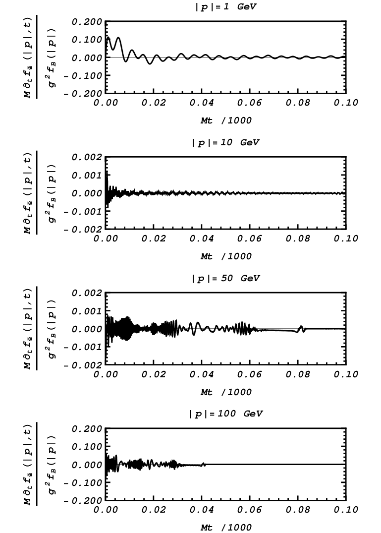
Figure 16: Numerical estimates of $\partial_{t}f_{\Phi}(|\mathbf{p}|,t)$, as a function of $Mt$, assuming that the $\chi$ statistical distribution functions $f^{(C)}_{\chi}(|\mathbf{p}|,t)$ on the RHS of the time evolution equation (IX.4) maintain their equilibrium Bose–Einstein form for all times.

Let us finally have a closer look at the early-time behavior that immediately follows after the switching on of the interactions. We expect that this prompt behavior is dominated by the ultra-violet contribution to the phase-space integral on the RHS of (IX.4) due to the Heisenberg uncertainty principle. From Figure 13, we see that this shock regime contributes dominantly to the prompt evolution of the infra-red modes of $f_{\Phi}(|\mathbf{p}|,t)$. In this regime, we take $|\mathbf{p}|\>=\>0$ and $m\>=\>0$ in (IX.4) and introduce the ultra-violet cut-off $\Lambda$ in the limits of the phase-space integrals of the RHS. Assuming that the $\chi$ distribution functions are tempered, vanishing faster than a power law for large momenta, we may ignore their contribution in the ultra-violet limit. Hence, $\partial_{t}f_{\Phi}(|\mathbf{p}|=0,t)$ can be approximated by

$$\partial_{t}f_{\Phi}(|\mathbf{p}|=0,t)\ \sim\ -\frac{g^{2}}{32\pi^{3}M}\Big{(}\,1\>+\>2f_{\Phi}(|\mathbf{p}|=0,t)\,\Big{)}\lim_{\Lambda\>\to\>\infty}\mathrm{Si}^{2}(\Lambda t)\;.$$ (310)

Clearly, $\partial_{t}f_{\Phi}(|\mathbf{p}|=0,t)$ vanishes in the limit $t\>\ll\>1/\Lambda\>\to\>0$, as we expect. Expanding $\mathrm{Si}\,(\Lambda t)$ about $\Lambda t\>=\>0$, i.e. for times infinitesimally close to zero, we obtain

$$\partial_{t}f_{\Phi}(|\mathbf{p}|=0,t)\ \sim\ -\frac{g^{2}}{32\pi^{3}M}\Big{(}\,1\>+\>2f_{\Phi}(|\mathbf{p}|=0,0)\,\Big{)}\lim_{\Lambda\>\to\>\infty}(\Lambda t)^{2}\;.$$ (311)

For small but finite times, ultra-violet contributions are rapidly varying. It is apparent from this discussion and Figures 13 and 16 that the effect of the transient behavior of the system upon its subsequent dynamics is significant, since the quantum memories persist on long time scales $Mt\>\gg\>1$. We may therefore conclude that as opposed to other methods relying on a truncated gradient expansion, our approach consistently describes this highly-oscillatory and rapidly-evolving early-time behavior of the system.

IX.5 Inclusion of Thermal Masses

In this section, we describe how local thermal-mass corrections may be incorporated consistently into our approach.

The local part of the one-loop $\chi$ self-energy shown in Figure 4 has the explicit form

$$\Pi_{\chi}^{\mathrm{loc}(1)}(p,p^{\prime},\tilde{t}_{f};\tilde{t}_{i})\ =\ -\frac{\lambda}{2}(2\pi)^{4}\delta_{t}^{(4)}(p\>-\>p^{\prime})(2\pi\mu)^{2\epsilon}e^{i(p_{0}\>-\>p_{0}^{\prime})\tilde{t}_{f}}$$

$$\qquad\qquad\times\>\!\iint\!\!\frac{\mathrm{d}^{d}{k}}{(2\pi)^{d}}\,\frac{\mathrm{d}^{4}{k^{\prime}}}{(2\pi)^{4}}\;\bigg{(}\,\frac{i}{k^{2}\>-\>m^{2}\>+\>i\epsilon}(2\pi)^{4}\delta^{(4)}(k\>-\>k^{\prime})$$

$$\qquad\qquad+\>2\pi\delta(k^{2}\>-\>m^{2})|2k_{0}|^{1/2}\tilde{f}_{\chi}(k,k^{\prime},t)e^{i(k_{0}\>-\>k_{0}^{\prime})\tilde{t}_{f}}|2k_{0}^{\prime}|^{1/2}2\pi\delta({k^{\prime}}^{2}\>-\>m^{2})\,\bigg{)}\;,$$ (312)

with $d\>=\>4\>-\>2\epsilon$ (cf. Appendix F). The first term yields the standard zero-temperature UV divergence, which is usually removed by mass renormalization. The second term yields

$$\Pi_{\chi}^{\mathrm{loc}(1)}(p,p^{\prime},\tilde{t}_{f};\tilde{t}_{i})\ =\ -(2\pi)^{4}\delta_{t}^{(4)}(p\>-\>p^{\prime})e^{i(p_{0}\>-\>p_{0}^{\prime})\tilde{t}_{f}}m_{\mathrm{th}}^{2}(\tilde{t}_{f};\tilde{t}_{i})\;,$$ (313)

where the time-dependent thermal mass $m_{\mathrm{th}}(\tilde{t}_{f};\tilde{t}_{i})$, given by

$$m_{\mathrm{th}}^{2}(\tilde{t}_{f};\tilde{t}_{i})\ =\ \frac{\lambda}{2}\!\int\!\!\frac{\mathrm{d}^{3}{\mathbf{k}}}{(2\pi)^{3}}\,\frac{1}{\sqrt{2E_{\chi}(\mathbf{k})}}\int\!\!\frac{\mathrm{d}^{3}{\mathbf{k}^{\prime}}}{(2\pi)^{3}}\,\frac{1}{\sqrt{2E_{\chi}(\mathbf{k}^{\prime})}}$$

$$\qquad\times\>\Big{(}\,f_{\chi}(\mathbf{k},\mathbf{k}^{\prime},t)e^{i[E(\mathbf{k})\>-\>E(\mathbf{k}^{\prime})]\tilde{t}_{f}}\>+\>f^{C*}_{\chi}(-\mathbf{k},-\mathbf{k}^{\prime},t)e^{-i[E(\mathbf{k})\>-\>E(\mathbf{k}^{\prime})]\tilde{t}_{f}}\,\Big{)}\;,$$ (314)

is UV finite. Notice that a unique thermal mass may not be defined in the spatially inhomogeneous case due to the explicit dependence on $\tilde{t}_{f}$.

From the Schwinger–Dyson equation in (122), the inverse quasi-particle CTP propagator $\Delta^{-1}_{\chi,\,ab}(p,p^{\prime},\tilde{t}_{f};\tilde{t}_{i})$ of the complex scalar field $\chi$ takes the form

$$\Delta^{-1}_{\chi,\,ab}(p,p^{\prime},\tilde{t}_{f};\tilde{t}_{i})\ =\ (2\pi)^{4}\delta^{(4)}_{t}(p\>-\>p^{\prime})e^{i(p_{0}\>-\>p_{0}^{\prime})\tilde{t}_{f}}\Big{[}\Big{(}\,p^{\prime 2}\>-\>m_{\mathrm{th}}^{2}(\tilde{t}_{f};\tilde{t}_{i})\,\Big{)}\eta_{ab}\>+\>i\epsilon\mathbb{I}_{ab}\,\Big{]}\;,$$ (315)

in which we have assumed $m_{\mathrm{th}}(t)\>\gg\>m$. If the quartic $\chi$ self-interaction is switched on sufficiently long before $t\>=\>0$, then for $t\>\geq\>0$, we may replace the $\delta_{t}$ function in the inverse quasi-particle propagator (315) by an exact energy-conserving delta function. This imposition of energy conservation constitutes a quasi-particle approximation, allowing us to invert (315) exactly, using the arguments of Sections III.2 and IV.3, to obtain the following quasi-particle $\chi$ propagators:

$$\Delta^{0,\,ab}_{\chi}(p,p^{\prime},\tilde{t}_{f};\tilde{t}_{i})\ =\ \!\begin{bmatrix}\big{(}p^{2}\,-\,m_{\mathrm{th}}^{2}(\tilde{t}_{f};\tilde{t}_{i})\,+\,i\epsilon)^{-1}&-i2\pi\theta(-p_{0})\delta\big{(}p^{2}\,-\,m_{\mathrm{th}}^{2}(\tilde{t}_{f};\tilde{t}_{i})\big{)}\\ -i2\pi\theta(p_{0})\delta\big{(}p^{2}\,-\,m_{\mathrm{th}}^{2}(\tilde{t}_{f};\tilde{t}_{i})\big{)}&-\big{(}p^{2}\,-\,m_{\mathrm{th}}^{2}(\tilde{t}_{f};\tilde{t}_{i})\,-\,i\epsilon\big{)}^{-1}\end{bmatrix}\!(2\pi)^{4}\delta^{(4)}(p\,-\,p^{\prime})$$

$$\qquad-\>i2\pi|2p_{0}|^{1/2}\delta\big{(}p^{2}\,-\,m_{\mathrm{th}}^{2}(\tilde{t}_{f};\tilde{t}_{i})\big{)}\tilde{f}_{\chi}(p,p^{\prime},t)e^{i(p_{0}\,-\,p_{0}^{\prime})\tilde{t}_{f}}2\pi|2p_{0}^{\prime}|^{1/2}\delta\big{(}p^{\prime 2}\,-\,m_{\mathrm{th}}^{2}(\tilde{t}_{f};\tilde{t}_{i})\big{)}\!\begin{bmatrix}1&1\\ 1&1\end{bmatrix}\!\;.$$ (316)

If the subsystem $\mathscr{S}_{\chi}$ is in a state of thermodynamic equilibrium at the initial time $t\>=\>0$, the thermal mass reduces to the known result

$$m_{\mathrm{th}}^{2}(t\>=\>0)\ =\ \frac{\lambda T^{2}}{24}\;,$$ (317)

for $m\>=\>0$ and $\mu\>\ll\>T$. In order to describe completely the dynamics of the combined system $\mathscr{S}\>=\>\mathscr{S}_{\Phi}\>\cup\>\mathscr{S}_{\chi}$, we couple the evolution of the thermal mass $m_{\mathrm{th}}(t)$ to the perturbative time evolution equations (IX.4) and (IX.4) for the $\Phi$ and $\chi$ statistical distribution functions. This is achieved by differentiating (IX.5) with respect to $t$, such that

$$\partial_{t}m_{\mathrm{th}}(t)\ =\ \frac{\lambda}{2m_{\mathrm{th}}(t)}\!\int\!\!\frac{\mathrm{d}^{3}{\mathbf{k}}}{(2\pi)^{3}}\,\frac{1}{2E_{\chi}(\mathbf{k})}\;\frac{1}{2}\Big{(}\,\partial_{t}f_{\chi}(|\mathbf{k}|,t)\>+\>\partial_{t}f^{C}_{\chi}(|\mathbf{k}|,t)\,\Big{)}\;.$$ (318)

Here, $\partial_{t}f_{\chi}(|\mathbf{k}|,t)$ and $\partial_{t}f_{\chi}^{C}(|\mathbf{k}|,t)$ depend implicitly upon $m_{\mathrm{th}}(t)$ via the coupled first-order differential equations (IX.4) and (IX.4), derived using the quasi-particle $\chi$ propagators in (IX.5). On dimensional grounds, we may estimate that the leading contribution to $\partial_{t}m_{\mathrm{th}}(t)$ is of order $\lambda^{1/2}gT$. The latter estimate provides firm support that our time evolution equations may consistently incorporate thermal masses and so describe the main non-perturbative dynamics of the system.

X Conclusions

We have developed a new perturbative approach to non-equilibrium thermal quantum field theory. Our perturbative approach is based upon non-homogeneous free propagators and time-dependent vertices, which explicitly break space-time translational invariance and properly encode the dependence of the system on the time of observation. The forms of these propagators are constrained by fundamental field-theoretic requirements, such as CPT invariance of the action, Hermiticity properties of correlation functions, causality and unitarity. We have shown that our perturbative approach gives rise to time-dependent diagrammatic perturbation series, which are free of pinch singularities. The absence of these pinch singularities results from the systematic inclusion of finite-time effects and the proper consideration of the time of observation. We emphasize that this is achieved without invoking ad hoc prescriptions or effective resummations of finite widths. In our formalism, we have derived the new master time evolution equations (VII) and (VII) for particle number densities and statistical distribution functions, which are valid to all orders in perturbation theory and to all orders in gradient expansion. Furthermore, the master time evolution equations (VII) and (VII) respect $CPT$ invariance and are also invariant under time translations of the CTP contour. As opposed to other methods, in our perturbative approach, we do not need to employ quasi-particle approximation and no assumption is necessary about the separation of time scales.

We have shown how the effect of a finite time interval since the start of evolution of the system leads to violation of energy conservation, as dictated by the Heisenberg uncertainty principle. Our approach permits the systematic treatment of the pertinent generalized kinematics in this evanescent regime. We have found that the available phase space of $1\>\to\>2$ decays increases and would-be kinematically disallowed processes can still take place at early times, contributing significantly to our time evolution equations. Within a simple scalar model, we have illustrated that these kinematically forbidden evanescent processes are the $2\>\to\>1$ processes of Landau damping, as well as $3\to 0$ processes of total annihilation into the thermal bath. The processes of Landau damping and total annihilation have been shown to contribute promptly to the particle width, to a level as high as $20\%$. The switching on of the interactions leads to a quantum quench in the system, which manifests itself as a rapid change in both the particle width and the collision terms of the time evolution equations. These early-time effects give rise to an oscillating pattern, which persists even at later times. We have demonstrated that these late-time memory effects exhibit a non-Markovian evolution characterized by oscillations with time-dependent frequencies. The latter constitutes a distinctive feature of proper non-equilibrium dynamics, which is consistently predicted by our perturbative approach.

We note that the rapid transient behavior of the system makes the method of gradient expansion unsuitable for early times. We emphasize that in our approach no assumption was made as to the relative rate of thermalization of either the statistical or spectral behavior of the system. For the considered initial conditions of thermal equilibrium, we have found that the spectral evolution resulting from evanescent contributions is critical to the early-time statistical dynamics of the system. Consequently, it would have been inappropriate to assume a separation of time scales at early times. A more accurate numerical solution to our time evolution equations turns out to be computationally intensive and may be presented elsewhere.

Finite-time effects, which are systematically incorporated in our perturbative approach, are also relevant to many-body systems whenever a natural characteristic time scale for perturbations arises in such systems. Thus, in addition to possible applications to reheating and preheating, of particular interest are first-order phase transitions. For instance, such characteristic time scales result from the bubble wall velocity of nucleation in the electroweak phase transition, e.g. see Huber and Schmidt (2001); Huber and Sopena (2012). In the vicinity of the bubble wall, evanescent contributions may weaken the constraints of decay and inverse decay thresholds and so affect the washout phenomena and the generation of relic densities. This evanescent regime is particularly relevant to prethermalization Berges et al. (2004) and isotropization Berges et al. (2005) time scales, which are known to be shorter than the time scale of thermalization.

It is straightforward to generalize our perturbative approach to theories that include fermions and gauge fields. Thus, it would be very interesting to extend the classical approaches Sigl and Raffelt (1993); Boyanovsky and Ho (2007) to kinetic equations of particle mixing to non-homogeneous backgrounds, by including finite-time evanescent effects in line with the non-equilibrium formalism presented in this paper.

Appendix A Propagator Properties and Identities

In this appendix, we give a detailed summary of the transformation properties and identities that relate the various propagators defined in Section II. In detail, the pertinent two-point correlation functions for the complex scalar field $\chi$ are given by

$$i\Delta(x,y) \ \equiv\ \braket{[\,\chi(x),\ \chi^{{\dagger}}(y)\,]}\;,$$ (319a)

$$i\Delta_{1}(x,y) \ \equiv\ \braket{\{\,\chi(x),\ \chi^{{\dagger}}(y)\,\}}\;,$$ (319b)

$$i\Delta_{\mathrm{R}}(x,y) \ \equiv\ \theta(x_{0}\>-\>y_{0})i\Delta(x,y)\;,$$ (319c)

$$i\Delta_{\mathrm{A}}(x,y) \ \equiv\ -\theta(y_{0}\>-\>x_{0})i\Delta(x,y)\;,$$ (319d)

$$i\Delta_{\mathcal{P}}(x,y) \ \equiv\ \tfrac{1}{2}\varepsilon(x_{0}\>-\>y_{0})\braket{[\,\chi(x),\ \chi^{{\dagger}}(y)\,]}\;,$$ (319e)

$$i\Delta_{>}(x,y) \ \equiv\ \braket{\chi(x)\chi^{{\dagger}}(y)}\;,$$ (319f)

$$i\Delta_{<}(x,y) \ \equiv\ \braket{\chi^{{\dagger}}(y)\chi(x)}\;,$$ (319g)

$$i\Delta_{\mathrm{F}}(x,y) \ \equiv\ \braket{\,\mathrm{T}\,[\,\chi(x)\chi^{{\dagger}}(y)\,]}\;,$$ (319h)

$$i\Delta_{\mathrm{D}}(x,y) \ \equiv\ \braket{\bar{\,\mathrm{T}}\,[\,\chi(x)\chi^{{\dagger}}(y)\,]}\;.$$ (319i)

The definitions of the charge-conjugate propagators follow from the unitary transformation

$$U_{C}^{{\dagger}}\chi(x)U_{C} \ =\ \chi^{C}(x)\ =\ \eta\chi^{{\dagger}}(x)\;,$$ (320a)

$$U_{C}^{{\dagger}}\chi^{{\dagger}}(x)U_{C} \ =\ \chi^{C{\dagger}}(x)\ =\ \eta^{*}\chi(x)\;,$$ (320b)

where the complex phase $\eta$ satisfies $|\eta|^{2}\>=\>1$.

It follows from the definitions that the propagators satisfy the transformations listed below under charge- and Hermitian-conjugation:

$$\Delta(x,y) \ =\ -\Delta^{*}(y,x)\ =\ -\Delta^{C}(y,x)\;,$$ (321a)

$$\Delta_{1}(x,y) \ =\ -\Delta_{1}^{*}(y,x)\ =\ \Delta_{1}^{C}(y,x)\;,$$ (321b)

$$\Delta_{\mathcal{P}}(x,y) \ =\ \Delta_{\mathcal{P}}^{*}(y,x)\ =\ \Delta_{\mathcal{P}}^{C}(y,x)\;,$$ (321c)

$$\Delta_{\mathrm{R}}(x,y) \ =\ \Delta^{C*}_{\mathrm{R}}(x,y)\ =\ \Delta_{\mathrm{A}}^{*}(y,x)\ =\ \Delta^{C}_{\mathrm{A}}(y,x)\;,$$ (321d)

$$\Delta_{>}(x,y) \ =\ -\Delta_{>}^{*}(y,x)\ =\ \Delta^{C}_{<}(y,x)\ =\ -\Delta_{<}^{C*}(x,y)\;,$$ (321e)

$$\Delta_{\mathrm{F}}(x,y) \ =\ \Delta^{C}_{\mathrm{F}}(y,x)\ =\ -\Delta^{*}_{\mathrm{D}}(y,x)\ =\ -\Delta^{C*}_{\mathrm{D}}(x,y)\;,$$ (321f)

where the action of charge-conjugation is trivial in the case of a real scalar field. In the double momentum representation, these identities take the form:

$$\Delta(p,p^{\prime}) \ =\ -\Delta^{*}(p^{\prime},p)\ =\ -\Delta^{C}(-p^{\prime},-p)\;,$$ (322a)

$$\Delta_{1}(p,p^{\prime}) \ =\ -\Delta_{1}^{*}(p^{\prime},p)\ =\ \Delta_{1}^{C}(-p^{\prime},-p)\;,$$ (322b)

$$\Delta_{\mathcal{P}}(p,p^{\prime}) \ =\ \Delta_{\mathcal{P}}^{*}(p^{\prime},p)\ =\ \Delta_{\mathcal{P}}^{C}(-p^{\prime},-p)\;,$$ (322c)

$$\Delta_{\mathrm{R}}(p,p^{\prime}) \ =\ \Delta_{\mathrm{R}}^{C*}(-p,-p^{\prime})\ =\ \Delta_{\mathrm{A}}^{*}(p^{\prime},p)\ =\ \Delta^{C}_{\mathrm{A}}(-p^{\prime},-p)\;,$$ (322d)

$$\Delta_{>}(p,p^{\prime}) \ =\ -\Delta_{>}^{*}(p^{\prime},p)\ =\ \Delta_{<}^{C}(-p^{\prime},-p)\ =\ -\Delta_{<}^{C*}(-p,-p^{\prime})\;,$$ (322e)

$$\Delta_{\mathrm{F}}(p,p^{\prime}) \ =\ \Delta_{\mathrm{F}}^{C}(-p^{\prime},-p)\ =\ -\Delta_{\mathrm{D}}^{*}(p^{\prime},p)\ =\ -\Delta_{\mathrm{D}}^{C*}(-p,-p^{\prime})\;.$$ (322f)

Finally, in the Wigner representation, the propagators satisfy the following properties:

$$\Delta(q,X) \ =\ -\Delta^{*}(q,X)\ =\ -\Delta^{C}(-q,X)\;,$$ (323a)

$$\Delta_{1}(q,X) \ =\ -\Delta_{1}^{*}(q,X)\ =\ \Delta_{1}^{C}(-q,X)\;,$$ (323b)

$$\Delta_{\mathcal{P}}(q,X) \ =\ \Delta_{\mathcal{P}}^{*}(q,X)\ =\ \Delta_{\mathcal{P}}^{C}(-q,X)\;,$$ (323c)

$$\Delta_{\mathrm{R}}(q,X) \ =\ \Delta^{C*}_{\mathrm{R}}(-q,X)\ =\ \Delta_{\mathrm{A}}^{*}(q,X)\ =\ \Delta^{C}_{\mathrm{A}}(-q,X)\;,$$ (323d)

$$\Delta_{>}(q,X) \ =\ -\Delta_{>}^{*}(q,X)\ =\ \Delta_{<}^{C}(-q,X)\ =\ -\Delta_{<}^{C*}(-q,X)\;,$$ (323e)

$$\Delta_{\mathrm{F}}(q,X) \ =\ \Delta_{\mathrm{F}}^{C}(-q,X)\ =\ -\Delta^{*}_{\mathrm{D}}(q,X)\ =\ -\Delta^{C*}_{\mathrm{D}}(-q,X)\;.$$ (323f)

We also list the following set of useful identities:

$$\Delta(x,y) \ =\ \Delta_{>}(x,y)\>-\>\Delta_{<}(x,y)\ =\ \Delta_{\mathrm{R}}(x,y)\>-\>\Delta_{\mathrm{A}}(x,y)\;,$$ (324a)

$$\ =\ \varepsilon(x_{0}\>-\>y_{0})\Big{(}\,\Delta_{\mathrm{F}}(x,y)\>-\>\Delta_{\mathrm{D}}(x,y)\,\Big{)}\;,$$ (324b)

$$\Delta_{1}(x,y) \ =\ \Delta_{>}(x,y)\>+\>\Delta_{<}(x,y)\ =\ \Delta_{\mathrm{F}}(x,y)\>+\>\Delta_{\mathrm{D}}(x,y)\;,$$ (324c)

$$\Delta_{\mathrm{R}(\mathrm{A})}(x,y) \ =\ \Delta_{\mathrm{F}}(x,y)\>-\>\Delta_{<(>)}(x,y)\ =\ -\Delta_{\mathrm{D}}(x,y)\>+\>\Delta_{>(<)}(x,y)\;,$$ (324d)

$$\Delta_{\mathrm{F}(\mathrm{D})}(x,y) \ =\ \frac{1}{2}\Big{(}\,(-)2\Delta_{\mathcal{P}}(x,y)\>+\>\Delta_{>}(x,y)\>+\>\Delta_{<}(x,y)\,\Big{)}\;,$$ (324e)

$$\Delta_{\mathcal{P}}(x,y) \ =\ \frac{1}{2}\Big{(}\,\Delta_{\mathrm{R}}(x,y)\>+\>\Delta_{\mathrm{A}}(x,y)\,\Big{)}\ =\ \frac{1}{2}\Big{(}\,\Delta_{\mathrm{F}}(x,y)\>-\>\Delta_{\mathrm{D}}(x,y)\,\Big{)}.$$ (324f)

We note that analogous relations hold for the corresponding self-energies and that these identities and relations are true for free and resummed propagators.

Appendix B Correspondence between Imaginary and Real Time Formalisms

In this appendix, we briefly outline a number of relevant details of the Imaginary Time Formalism (ITF) of thermal field theory. These details are discussed in the context of the real scalar field theory introduced in Section II. Subsequently, we identify the correspondence of the ITF $\Phi$-scalar propagator and its one-loop non-local self-energy with results calculated explicitly in real time, using the CTP formalism of Section III in the equilibrium limit discussed in Section V.

The equilibrium density operator $\rho_{\mathrm{eq}}$ in (167) permits a path-integral representation in negative imaginary time. The ITF generating functional is

$$\mathcal{Z}[J]\ =\ \!\int\![\mathrm{d}{\Phi}]\,\exp\!\bigg{(}-\bar{S}[\Phi]\>+\>\!\int_{0}^{\beta}\!\!\mathrm{d}{\tau_{x}}\int\!\mathrm{d}^{3}{\mathbf{x}}\;J(\bar{x})\Phi(\bar{x})\bigg{)}\;,$$ (325)

with action

$$\bar{S}[\Phi]\ =\ \!\int_{0}^{\beta}\!\!\mathrm{d}{\tau_{x}}\int\!\mathrm{d}^{3}{\mathbf{x}}\;\Big{(}\,\tfrac{1}{2}\partial_{\mu}\Phi(\bar{x})\partial_{\mu}\Phi(\bar{x})\>+\>\tfrac{1}{2}M^{2}\Phi^{2}(\bar{x})\>+\>\tfrac{1}{3!}g\Phi^{3}(\bar{x})\>+\>\tfrac{1}{4!}\lambda\Phi^{4}(\bar{x})\,\Big{)}\;.$$ (326)

We emphasize the restricted domain of integration over the imaginary time $\tau_{x}\>\in\>[0,\ \beta]$. Four-dimensional Euclidean space-time coordinates are denoted by a horizontal bar, i.e. $\bar{x}_{\mu}\>\equiv\>(\tau_{x},\mathbf{x})$. In the limit $\beta\>\to\>\infty$, (325) is precisely the Wick rotation to Euclidean space-time of the Minkowski-space generating functional via the analytic continuation $x_{0}\>\to\>-i\tau_{x}$.

The free imaginary-time propagator $\bar{\Delta}^{0}$ may be written as follows:

$$\bar{\Delta}^{0}(\bar{x}-\bar{y})\ =\ \frac{1}{\beta}\sum_{\ell\>=\>-\infty}^{+\infty}\int\!\!\frac{\mathrm{d}^{3}{\mathbf{p}}}{(2\pi)^{3}}\;e^{i[\omega_{\ell}(\tau_{x}\>-\>\tau_{y})\>+\>\mathbf{p}\cdot(\mathbf{x}\>-\>\mathbf{y})]}\bar{\Delta}_{0}(i\omega_{\ell},\mathbf{p})\;,$$ (327)

where

$$\bar{\Delta}^{0}(i\omega_{\ell},\mathbf{p})\ =\ \frac{1}{\omega_{\ell}^{2}\>+\>\mathbf{p}^{2}\>+\>M^{2}}$$ (328)

is the so-called Matsubara propagator. The discrete Matsubara frequencies $\omega_{\ell}\>=\>2\pi\ell/\beta$, $\ell\>\in\>\mathbb{Z}$, arise from the periodicity of the imaginary time direction in order to satisfy the KMS relation [cf. (176)]

$$\bar{\Delta}^{0}(\bar{x}-\bar{y})\ =\ \bar{\Delta}^{0}(\bar{x}-\bar{y}+\beta)\;.$$ (329)

The resummed Matsubara propagator is given by the imaginary-time Schwinger–Dyson equation

$$\bar{\Delta}^{-1}(i\omega_{\ell},\mathbf{p})\ =\ \bar{\Delta}^{0,\,-1}(i\omega_{\ell},\mathbf{p})\>+\>\bar{\Pi}(i\omega_{\ell},\mathbf{p})\;,$$ (330)

where $\bar{\Pi}(\omega_{\ell},\mathbf{p})$ is the imaginary-time self-energy. Equation (330) may be inverted directly to obtain

$$\bar{\Delta}(i\omega_{\ell},\mathbf{p})\ =\ \frac{1}{\omega_{\ell}^{2}\>+\>\mathbf{p}^{2}\>+\>M^{2}\>+\>\bar{\Pi}(i\omega_{\ell},\mathbf{p})}\;.$$ (331)

The free Matsubara propagator in (328) may also be written in the following spectral representation:

$$\bar{\Delta}^{0}(i\omega_{\ell},\mathbf{p})\ =\ -i\!\int\!\frac{\mathrm{d}{k_{0}}}{2\pi}\;\frac{\Delta^{0}(k_{0},\mathbf{p})}{i\omega_{\ell}\>-\>k_{0}}\;,$$ (332)

where

$$i\Delta^{0}(k_{0},\mathbf{p})\ =\ 2\pi\varepsilon(k_{0})\delta(k_{0}^{2}\>-\>\mathbf{p}^{2}\>-\>M^{2})$$ (333)

is the single-momentum representation of the free Pauli–Jordan propagator, consistent with (16a). Making the analytic continuation $i\omega_{\ell}\>\to\>p_{0}\>+\>i\epsilon$ to real frequencies and comparing with the spectral representation of the retarded propagator $\Delta_{\mathrm{R}}$ in (22), we may establish the correspondence

$$\bar{\Delta}^{0}(i\omega_{\ell}\to p_{0}+i\epsilon,\mathbf{p})\ =\ -\Delta^{0}_{\mathrm{R}}(p)\;.$$ (334)

This correspondence must also hold for the resummed Matsubara propagator $\bar{\Delta}$ via (330). As such, the analytic continuation of the ITF self-energy $\bar{\Pi}$,

$$\bar{\Pi}(i\omega_{\ell}\to p_{0}+i\epsilon,\mathbf{p})\ =\ -\Pi_{\mathrm{R}}(p)\;,$$ (335)

yields the equilibrium retarded self-energy $\Pi_{\mathrm{R}}$.

Thus, in thermodynamic equilibrium, an exact correspondence can be established between the ITF and the real-time approach of the CTP formalism, by means of retarded propagators and self-energies. The full complement of propagators exhibited in Table 2 and the corresponding self-energies may be obtained using the constraints of causality (24) and unitarity (28) in combination with the KMS relation (177) and the condition of detailed balance (186). The relationships between the retarded and CTP propagators and self-energies are listed explicitly in (180) and (187).

To illustrate the correspondence in (335), we consider the one-loop bubble diagram of the real scalar theory in (1). The real and imaginary parts of the retarded self-energy $\Pi_{\mathrm{R}}$ may be calculated in the CTP formalism from the time-ordered $\Pi$ and positive-frequency Wightman $\Pi_{>}$ self-energies, respectively, using the relations in (187).

The real part of the one-loop retarded self-energy $\Pi_{\mathrm{R}}^{(1)}$ is given by

$$\mathrm{Re}\,\Pi_{\mathrm{R}}^{(1)}(p)\ =\ \mathrm{Re}\bigg{[}-i\frac{(-ig)^{2}}{2}\!\int\!\!\frac{\mathrm{d}^{4}{k}}{(2\pi)^{4}}\;i\Delta_{\mathrm{F}}^{0}(k)i\Delta_{\mathrm{F}}^{0}(p-k)\bigg{]}\;,$$ (336)

where $i\Delta^{0}_{\mathrm{F}}(k)$ is the equilibrium CTP Feynman propagator in (171a). Explicitly, we have

$$\mathrm{Re}\,\Pi_{\mathrm{R}}^{(1)}(p)\ =\ -\frac{g^{2}}{2}\int\!\!\frac{\mathrm{d}^{3}{\mathbf{k}}}{(2\pi)^{3}}\;\frac{1}{4E_{1}E_{2}}\bigg{[}\,\sum_{\alpha_{1}\>=\>\pm 1}\;\int\limits_{(p-k)^{2}\neq M^{2}}\!\!\!\!\!\!\!\!\!\!\!\mathrm{d}{k_{0}}\;\frac{2E_{2}}{(p-k)^{2}-M^{2}}\,\delta\big{(}k_{0}\>-\>\alpha_{1}E_{1}\big{)}\Big{(}\,\tfrac{1}{2}\>+\>f_{\mathrm{B}}(k_{0})\,\Big{)}$$

$$\qquad+\>\sum_{\alpha_{2}\>=\>\pm 1}\;\int\limits_{k^{2}\neq M^{2}}\!\!\!\!\!\!\mathrm{d}{k_{0}}\;\frac{2E_{1}}{k^{2}-M^{2}}\,\delta\big{(}p_{0}\>-\>k_{0}\>-\>\alpha_{2}E_{2}\big{)}\Big{(}\,\tfrac{1}{2}\>+\>f_{\mathrm{B}}(p_{0}-k_{0})\,\Big{)}\bigg{]}\;,$$ (337)

where $E_{1}\>\equiv\>E(\mathbf{k})$ and $E_{2}\>\equiv\>E(\mathbf{p}-\mathbf{k})$. The integral subscripts remind us that the integration around the on-shell poles is understood in the Cauchy principal value sense. Integration over $k_{0}$ yields the result

$$\mathrm{Re}\,\Pi_{\mathrm{R}}^{(1)}(p)\ =\ -\frac{g^{2}}{2}\sum_{\{\alpha\}}\!\int\!\!\frac{\mathrm{d}^{3}{\mathbf{k}}}{(2\pi)^{3}}\,\frac{\alpha_{1}\alpha_{2}}{4E_{1}E_{2}}\,\frac{1\>+\>f_{\mathrm{B}}(\alpha_{1}E_{1})\>+\>f_{\mathrm{B}}(\alpha_{2}E_{2})}{p_{0}\>-\>\alpha_{1}E_{1}\>-\>\alpha_{2}E_{2}}\;,$$ (338)

where we have used the short-hand notation $\{\alpha\}$ to denote summation over $\alpha_{1},\ \alpha_{2}\>=\>\pm 1$.

The one-loop positive-frequency Wightman self-energy is given by

$$i\Pi^{(1)}_{>}(p)\ =\ \frac{(-ig)^{2}}{2}\!\int\!\!\frac{\mathrm{d}^{4}{k}}{(2\pi)^{4}}\;i\Delta^{0}_{>}(k)i\Delta^{0}_{>}(p-k)\;.$$ (339)

Using the signum form of the equilibrium positive-frequency Wightman propagator $i\Delta^{0}_{>}(k)$ in (171b), we obtain

$$\Pi^{(1)}_{>}(p)\ =\ i\pi g^{2}\sum_{\{\alpha\}}\int\!\!\frac{\mathrm{d}^{3}{\mathbf{k}}}{(2\pi)^{3}}\int\!\mathrm{d}{k_{0}}\;\frac{\alpha_{1}\alpha_{2}}{4E_{1}E_{2}}\,\delta(k_{0}\>-\>\alpha_{1}E_{1})\delta(p_{0}\>-\>k_{0}\>-\>\alpha_{2}E_{2})\Big{(}\,1\>+\>f_{\mathrm{B}}(k_{0})\,\Big{)}\Big{(}\,1\>+\>f_{\mathrm{B}}(p_{0}-k_{0})\,\Big{)}\;.$$ (340)

The product of Bose–Einstein distributions in (340) satisfies the following relation:

$$f_{\mathrm{B}}(k_{0})f_{\mathrm{B}}(p_{0}-k_{0})\ =\ f_{\mathrm{B}}(p_{0})\,\Big{(}\,1\>+\>f_{\mathrm{B}}(k_{0})\>+\>f_{\mathrm{B}}(p_{0}-k_{0})\,\Big{)}\;.$$ (341)

Thus, upon integration over $k_{0}$, we find

$$\Pi^{(1)}_{>}(p)\ =\ i\pi g^{2}\Big{(}\,1\>+\>f_{\mathrm{B}}(p_{0})\,\Big{)}\sum_{\{\alpha\}}\int\!\!\frac{\mathrm{d}^{3}{\mathbf{k}}}{(2\pi)^{3}}\;\frac{\alpha_{1}\alpha_{2}}{4E_{1}E_{2}}\,\delta(p_{0}\>-\>\alpha_{1}E_{1}\>-\>\alpha_{2}E_{2})\Big{(}\,1\>+\>f_{\mathrm{B}}(\alpha_{1}E_{1})\>+\>f_{\mathrm{B}}(\alpha_{2}E_{2})\,\Big{)}\;.$$ (342)

Using the relation in (187c), the imaginary part of the one-loop retarded self-energy may then be written down as

$$\mathrm{Im}\,\Pi_{\mathrm{R}}^{(1)}(p)\ =\ \frac{\pi g^{2}}{2}\sum_{\{\alpha\}}\int\!\!\frac{\mathrm{d}^{3}{\mathbf{k}}}{(2\pi)^{3}}\;\frac{\alpha_{1}\alpha_{2}}{4E_{1}E_{2}}\,\delta(p_{0}\>-\>\alpha_{1}E_{1}\>-\>\alpha_{2}E_{2})\Big{(}\,1\>+\>f_{\mathrm{B}}(\alpha_{1}E_{1})\>+\>f_{\mathrm{B}}(\alpha_{2}E_{2})\,\Big{)}\;.$$ (343)

In the ITF, the one-loop self-energy is given by

$$-\bar{\Pi}^{(1)}(i\omega_{\ell},\mathbf{p})\ =\ \frac{(-g)^{2}}{2\beta}\sum_{n\>=\>-\infty}^{+\infty}\int\!\!\frac{\mathrm{d}^{3}{\mathbf{k}}}{(2\pi)^{3}}\;\bar{\Delta}(i\omega_{n},\mathbf{k})\bar{\Delta}(i(\omega_{\ell}-\omega_{n}),\mathbf{p}-\mathbf{k})\;.$$ (344)

After performing the summation over $n$ (see for instance Le Bellac (2000)), we obtain

$$\bar{\Pi}^{(1)}(i\omega_{\ell},\mathbf{p})\ =\ \frac{g^{2}}{2}\sum_{\{\alpha\}}\int\!\!\frac{\mathrm{d}^{3}{\mathbf{k}}}{(2\pi)^{3}}\;\frac{\alpha_{1}\alpha_{2}}{4E_{1}E_{2}}\,\frac{1\>+\>f_{\mathrm{B}}(\alpha_{1}E_{1})\>+\>f_{\mathrm{B}}(\alpha_{2}E_{2})}{i\omega_{\ell}\>-\>\alpha_{1}E_{1}\>-\>\alpha_{2}E_{2}}\;.$$ (345)

Making the analytic continuation $i\omega_{\ell}\>\to\>p_{0}\>+\>i\epsilon$ and subsequently extracting the real and imaginary parts, the result in (345) agrees with (338) and (343) via the correspondence in (335).

Appendix C The Complex Scalar Field

This appendix describes the generalization of the results in Sections IV.3 and V to the case of a complex scalar field $\chi$. In particular, we derive the full complement of non-homogeneous free propagators and expand upon the ITF correspondence identified in Appendix B.

Our starting point is the complex-scalar Lagrangian

$$\mathcal{L}(x)\ =\ \partial_{\mu}\chi^{{\dagger}}(x)\partial^{\mu}\chi(x)\>-\>m^{2}\chi^{{\dagger}}(x)\chi(x)\>-\>\tfrac{1}{4}\lambda\big{[}\chi^{{\dagger}}(x)\chi(x)\big{]}^{2}\;.$$ (346)

In analogy to (11), the complex scalar field $\chi(x)$ may be written in the interaction picture as

$$\chi(x;\tilde{t}_{i})\ =\ \!\int\!\mathrm{d}{\Pi_{\mathbf{p}}}\;\Big{(}\,a(\mathbf{p},0;\tilde{t}_{i})e^{-iE(\mathbf{p})x_{0}}e^{i\mathbf{p}\cdot\mathbf{x}}\>+\>b^{{\dagger}}(\mathbf{p},0;\tilde{t}_{i})e^{iE(\mathbf{p})x_{0}}e^{-i\mathbf{p}\cdot\mathbf{x}}\,\Big{)}\;,$$ (347)

where $a^{{\dagger}}(\mathbf{p},0;\tilde{t}_{i})$ and $a(\mathbf{p},0;\tilde{t}_{i})$ ($b^{{\dagger}}(\mathbf{p},0;\tilde{t}_{i})$ and $b(\mathbf{p},0;\tilde{t}_{i})$) are the interaction-picture particle (anti-particle) creation and annihilation operators, respectively. Under $C$-conjugation [cf. (320a)] these creation and annihilation operators satisfy the transformations

$$U_{C}^{{\dagger}}\,a(\mathbf{p},\tilde{t};\tilde{t}_{i})U_{C}\ =\ \eta b(\mathbf{p},\tilde{t};\tilde{t}_{i})\;,\qquad U_{C}^{{\dagger}}\,b^{{\dagger}}(\mathbf{p},\tilde{t};\tilde{t}_{i})U_{C}\ =\ \eta a^{{\dagger}}(\mathbf{p},\tilde{t};\tilde{t}_{i})\;.$$ (348)

Introducing the four-dimensional LIPS measure from (3), the field operator (347) and its Hermitian conjugate may be recast in the form

$$\chi(x;\tilde{t}_{i})\ =\ \!\int\!\!\frac{\mathrm{d}^{4}{p}}{(2\pi)^{4}}\;e^{-ip\cdot x}\,\chi(p;\tilde{t}_{i})\;,\qquad\chi^{{\dagger}}(x;\tilde{t}_{i})\ =\ \!\int\!\!\frac{\mathrm{d}^{4}{p}}{(2\pi)^{4}}\;e^{-ip\cdot x}\,\chi^{{\dagger}}(-p;\tilde{t}_{i})\;,$$ (349)

where the Fourier amplitudes are given by

$$\chi(p;\tilde{t}_{i})\ =\ 2\pi\delta(p^{2}\>-\>m^{2})\Big{(}\,\theta(p_{0})a(\mathbf{p},0;\tilde{t}_{i})\>+\>\theta(-p_{0})b^{{\dagger}}(-\mathbf{p},0;\tilde{t}_{i})\,\Big{)}\;.$$ (350)

For the real scalar field, the quantization scheme was only dependent on the restriction placed upon the form of the field commutator. In the case of the complex scalar field, we have two degrees of freedom to fix. Thus, we begin with the following two commutators of interaction-picture fields:

$$\big{[}\,\chi(x),\ \chi(y)\,\big{]}\ =\ 0\;,\qquad\big{[}\,\chi(x),\ \chi^{{\dagger}}(y)\,\big{]}\ =\ i\Delta^{0}(x,y;m^{2})\;,$$ (351)

where the Pauli–Jordan propagator has precisely the form in (15). In analogy to the real scalar field, we may derive from (351) the equal-time commutation relations

$$i\Delta^{0}(x,y;m^{2})\big{|}_{x^{0}\>=\>y^{0}\>=\>\tilde{t}} \ =\ \big{[}\,\chi(\tilde{t},\mathbf{x}),\ \chi^{{\dagger}}(\tilde{t},\mathbf{y})\,\big{]}\ =\ 0\;,$$ (352a)

$$\partial_{x_{0}}i\Delta^{0}(x,y;m^{2})\big{|}_{x^{0}\>=\>y^{0}\>=\>\tilde{t}} \ =\ \big{[}\,\pi^{{\dagger}}(\tilde{t},\mathbf{x}),\ \chi^{{\dagger}}(\tilde{t},\mathbf{y})\,\big{]}\ =\ -i\delta^{(3)}(\mathbf{x}\>-\>\mathbf{y})\;,$$ (352b)

$$\partial_{y_{0}}i\Delta^{0}(x,y;m^{2})\big{|}_{x^{0}\>=\>y^{0}\>=\>\tilde{t}} \ =\ \big{[}\,\chi(\tilde{t},\mathbf{x}),\ \pi(\tilde{t},\mathbf{y})\,\big{]}\ =\ i\delta^{(3)}(\mathbf{x}\>-\>\mathbf{y})\;,$$ (352c)

$$\partial_{x_{0}}\partial_{y_{0}}i\Delta^{0}(x,y;m^{2})\big{|}_{x^{0}\>=\>y^{0}\>=\>\tilde{t}} \ =\ \big{[}\,\pi^{{\dagger}}(\tilde{t},\mathbf{x}),\ \pi(\tilde{t},\mathbf{y})\,\big{]}\ =\ 0\;,$$ (352d)

where $\pi(x)\>=\>\partial_{x_{0}}\chi^{{\dagger}}(x)$ is the conjugate momentum operator. The particle and anti-particle creation and annihilation operators necessarily satisfy the algebra

$$\big{[}\,a(\mathbf{p},\tilde{t}),\ a^{{\dagger}}(\mathbf{p}^{\prime},\tilde{t}^{\prime})\,\big{]}\ =\ \big{[}\,b(\mathbf{p},\tilde{t}),\ b^{{\dagger}}(\mathbf{p}^{\prime},\tilde{t}^{\prime})\,\big{]}\ =\ (2\pi)^{3}2E(\mathbf{p})\delta^{(3)}(\mathbf{p}\>-\>\mathbf{p}^{\prime})e^{-iE(\mathbf{p})(\tilde{t}\>-\>\tilde{t}^{\prime})}\;,$$ (353)

with all other commutators vanishing. We stress again that the phase factor $e^{-iE(\mathbf{p})(\tilde{t}\>-\>\tilde{t}^{\prime})}$ on the RHS of (353) has appeared due to the difference in microscopic times of the interaction-picture creation and annihilation operators.

In addition to the $C$-conserving propagators listed in Appendix A, we may also define $C$-violating propagators. As an example, the $C$-violating Hadamard propagator $\Delta_{1\not{C}}(x,y)$ would read:

$$i\Delta_{1\not{C}}(x,y)\ =\ \braket{\,\{\,\chi(x),\ \chi(y)\,\}\,}\;,$$ (354)

which satisfies

$$\Delta_{1\not{C}}(x,y)\ =\ \Delta_{1\not{C}}(y,x)\ =\ -\eta^{2}\Delta^{C*}_{1\not{C}}(x,y)\;.$$ (355)

This Hadamard correlation function may, in general, be non-zero for early times, thus permitting extra $C$-violating evanescent processes in addition to those described in Section IX.

In analogy to (143), we write the following set of EEVs of two-point products of particle and anti-particle creation and annihilation operators:

$$\braket{a^{{\dagger}}(\mathbf{p}^{\prime},\tilde{t}_{f};\tilde{t}_{i})a(\mathbf{p},\tilde{t}_{f};\tilde{t}_{i})}_{t} \ =\ 2\mathscr{E}(\mathbf{p},\mathbf{p}^{\prime})f(\mathbf{p},\mathbf{p}^{\prime},t)\;,$$ (356a)

$$\braket{b(\mathbf{p}^{\prime},\tilde{t}_{f};\tilde{t}_{i})a(\mathbf{p},\tilde{t}_{f};\tilde{t}_{i})}_{t} \ =\ 2\mathscr{E}(\mathbf{p},\mathbf{p}^{\prime})g(\mathbf{p},\mathbf{p}^{\prime},t)\;,$$ (356b)

$$\braket{a(\mathbf{p}^{\prime},\tilde{t}_{f};\tilde{t}_{i})a(\mathbf{p},\tilde{t}_{f};\tilde{t}_{i})}_{t} \ =\ 2\mathscr{E}(\mathbf{p},\mathbf{p}^{\prime})h(\mathbf{p},\mathbf{p}^{\prime},t)\;,$$ (356c)

$$\braket{b^{{\dagger}}(\mathbf{p}^{\prime},\tilde{t}_{f};\tilde{t}_{i})a(\mathbf{p},\tilde{t}_{f};\tilde{t}_{i})}_{t} \ =\ 2\mathscr{E}(\mathbf{p},\mathbf{p}^{\prime})d(\mathbf{p},\mathbf{p}^{\prime},t)\;,$$ (356d)

where the remaining EEVs are obtained by Hermitian and charge conjugation. The four statistical distribution functions $f,\ g,\ h,\ d$ satisfy the following identities:

$$f(\mathbf{p},\mathbf{p}^{\prime},t) \ =\ f^{*}(\mathbf{p}^{\prime},\mathbf{p},t)\;,$$ (357a)

$$g(\mathbf{p},\mathbf{p}^{\prime},t) \ =\ g^{C}(\mathbf{p}^{\prime},\mathbf{p},t)\;,$$ (357b)

$$h(\mathbf{p},\mathbf{p}^{\prime},t) \ =\ h(\mathbf{p}^{\prime},\mathbf{p},t)\;,$$ (357c)

$$d(\mathbf{p},\mathbf{p}^{\prime},t) \ =\ \eta^{2}d^{C*}(\mathbf{p}^{\prime},\mathbf{p},t)\;.$$ (357d)

The non-homogeneous free propagators of the complex scalar field $\chi$ may be written as listed in Table 2 with the substitution of the following ensemble function:

$$\tilde{f}(p,p^{\prime},t)\ =\ \theta(p_{0})\theta(p_{0}^{\prime})f(\mathbf{p},\mathbf{p}^{\prime},t)\>+\>\theta(-p_{0})\theta(-p_{0}^{\prime})f^{C*}(-\mathbf{p},-\mathbf{p}^{\prime},t)$$

$$\qquad+\>\theta(p_{0})\theta(-p_{0}^{\prime})g(\mathbf{p},-\mathbf{p}^{\prime},t)\>+\>\theta(-p_{0})\theta(p_{0}^{\prime})g^{C*}(-\mathbf{p},\mathbf{p}^{\prime},t)\;,$$ (358)

satisfying the relations: $\tilde{f}(p,p^{\prime},t)\>=\>\tilde{f}^{C}(-p^{\prime},-p,t)\>=\>\tilde{f}^{C*}(-p,-p^{\prime},t)$ in accordance with (322). The free $C$-violating Hadamard propagator $\Delta^{0}_{1\not{C}}(p,p^{\prime},\tilde{t}_{f};\tilde{t}_{i})$, defined in (354), may be written down as

$$\Delta_{1\not{C}}(p,p^{\prime},\tilde{t}_{f};\tilde{t}_{i})\ =\ -i2\pi\delta(p^{2}\>-\>m^{2})|2p_{0}|^{1/2}2\tilde{d}(p,p^{\prime},t)e^{i(p_{0}\>-\>p_{0}^{\prime})\tilde{t}_{f}}|2p_{0}^{\prime}|^{1/2}2\pi\delta(p^{\prime 2}\>-\>m^{2})\;,$$ (359)

where we have defined the $C$-violating ensemble function $\tilde{d}(p,p^{\prime},t)$. Evaluating the EEVs directly, we find

$$\tilde{d}(p,p^{\prime},t)\ =\ \theta(p_{0})\theta(p_{0}^{\prime})d(\mathbf{p},\mathbf{p}^{\prime},t)\>+\>\theta(-p_{0})\theta(-p_{0}^{\prime})\eta^{2}d^{C*}(-\mathbf{p},-\mathbf{p}^{\prime},t)$$

$$\qquad+\>\theta(p_{0})\theta(-p_{0}^{\prime})h(\mathbf{p},-\mathbf{p}^{\prime},t)\>+\>\theta(-p_{0})\theta(p_{0}^{\prime})\eta^{2}h^{C*}(-\mathbf{p},\mathbf{p}^{\prime},t)\;.$$ (360)

satisfying the relations: $\tilde{d}(p,p^{\prime},t)\>=\>\tilde{d}^{C}(-p^{\prime},-p,t)\>=\>\eta^{2}\tilde{d}^{C*}(-p,-p^{\prime},t)$.

The inclusion of the $C$-violating distribution functions requires the addition of the $C$-violating source $l_{ab}$ to the expansion of the kernel of the density operator in the CTP generating functional, according to our discussion in Section IV.1. Omitting the $t$ dependence of the sources for notational convenience, the CTP generating functional for the complex scalar field $\chi$ takes the form

$$\mathcal{W}[j_{a},k_{ab},l_{ab}] \ =\ -i\hbar\ln\!\iint\![\mathrm{d}{(\chi^{a{\dagger}},\chi^{a})}]\exp\!\bigg{\{}\frac{i}{\hbar}\bigg{[}S\big{[}\chi^{a{\dagger}},\chi^{a}\big{]}\>+\>\!\int_{\Omega_{t}}\!\mathrm{d}^{4}{x}\;\Big{(}\,j_{a}^{{\dagger}}(x)\chi^{a}(x)\>+\>\chi_{a}^{{\dagger}}(x)j^{a}(x)\,\Big{)}$$

$$\qquad+\>\!\iint_{\Omega_{t}}\!\mathrm{d}^{4}{x}\,\mathrm{d}^{4}{x^{\prime}}\;\Big{(}\,\chi^{a{\dagger}}(x)k_{ab}(x,x^{\prime})\chi^{b}(x^{\prime})$$

$$\qquad+\>\frac{1}{2}\,\chi^{a}(x)l_{ab}^{{\dagger}}(x,x^{\prime})\chi^{b}(x^{\prime})\>+\>\frac{1}{2}\,\chi^{a{\dagger}}(x)l_{ab}(x,x^{\prime})\chi^{b{\dagger}}(x^{\prime})\,\Big{)}\>+\>\cdots\bigg{]}\bigg{\}}\;.$$ (361)

The bi-local sources $k_{ab}$ and $l_{ab}$ necessarily satisfy the identities

$$k_{ab}(x,x^{\prime})\ =\ k_{ba}^{{\dagger}}(x^{\prime},x)\;,\qquad l_{ab}(x,x^{\prime})\ =\ l_{ba}(x^{\prime},x)\;,$$ (362)

to ensure that the exponent of the generating functional is $CPT$-invariant. The subsequent derivation of the effective action then follows analogously to Section IV.

The Lagrangian in (346) is invariant under the global $U(1)$ transformation

$$\chi(x)\ \to\ \chi^{\prime}(x)\ =\ e^{-i\alpha}\,\chi(x)\;,\qquad\chi^{{\dagger}}(x)\ \to\ \chi^{\prime{\dagger}}(x)\ =\ e^{i\alpha}\,\chi^{{\dagger}}(x)\;,$$ (363)

entailing the conserved Noether current

$$j_{\mu}(x)\ =\ i\Big{(}\,\chi^{{\dagger}}(x)\partial_{\mu}\chi(x)\>-\>\big{(}\partial_{\mu}\chi^{{\dagger}}(x)\big{)}\chi(x)\,\Big{)}\;,$$ (364)

with corresponding conserved charge

$$:\mathcal{Q}(x_{0}):\ =\ \!\int\!\mathrm{d}^{3}{\mathbf{x}}\;:j_{0}(x):\ =\ \!\int\!\mathrm{d}{\Pi_{\mathbf{p}}}\;\Big{(}\,a^{{\dagger}}(\mathbf{p},0)a(\mathbf{p},0)\>-\>b^{{\dagger}}(\mathbf{p},0)b(\mathbf{p},0)\,\Big{)}\;,$$ (365)

where $:\ :$ denotes normal ordering. The existence of this conserved charge necessitates the introduction of a chemical potential $\mu$ and, as such, the equilibrium density operator is of the grand-canonical form

$$\rho(\beta,\mu)\ =\ e^{-\beta(H-\mu Q)}\;.$$ (366)

In the presence of this chemical potential, the KMS relation in (176) generalizes to

$$\Delta_{>}(x^{0}-y^{0},\mathbf{x}-\mathbf{y})\ =\ e^{-\beta\mu}\Delta_{<}(x^{0}-y^{0}+i\beta,\mathbf{x}-\mathbf{y})$$ (367)

or, in the momentum representation,

$$\Delta_{>}(p)\ =\ e^{\beta(p_{0}-\mu)}\Delta_{<}(p)\;.$$ (368)

Proceeding as in Section III, we find that the final constraint on $\tilde{f}(p)$, generalizing (178), is

$$\tilde{f}(p)\ =\ \theta(p_{0})f_{\mathrm{B}}(p_{0})\>+\>\theta(-p_{0})f^{C}_{\mathrm{B}}(-p_{0})\;,$$ (369)

where $f^{(C)}_{\mathrm{B}}(p_{0})\>=\>(e^{\beta[p_{0}-(+)\mu]}-1)^{-1}$ is the particle (anti-particle) Bose–Einstein distribution function. In equilibrium, translational invariance is restored and the elements of the free CTP propagator may be written in the single momentum representations

$$i\Delta^{0}_{\mathrm{F}}(p) \ =\ i\Big{(}\,p^{2}\>-\>m^{2}\>+\>i\epsilon\,\Big{)}^{-1}\>+\>2\pi\,\Big{(}\,\theta(p_{0})f_{\mathrm{B}}(p_{0})\>+\>\theta(-p_{0})f^{C}_{\mathrm{B}}(-p_{0})\,\Big{)}\delta(p^{2}\>-\>m^{2})\;,$$ (370a)

$$i\Delta^{0}_{>}(p) \ =\ 2\pi\Big{[}\,\theta(p_{0})\Big{(}\,1\>+\>f_{\mathrm{B}}(p_{0})\,\Big{)}\>+\>\theta(-p_{0})f^{C}_{\mathrm{B}}(-p_{0})\,\Big{]}\delta(p^{2}\>-\>m^{2})\;,$$ (370b)

$$i\Delta^{0}_{<}(p) \ =\ 2\pi\Big{[}\,\theta(p_{0})f_{\mathrm{B}}(p_{0})\>+\>\theta(-p_{0})\Big{(}\,1\>+\>f^{C}_{\mathrm{B}}(-p_{0})\,\Big{)}\Big{]}\delta(p^{2}\>-\>m^{2})\;.$$ (370c)

In order to define the ITF generating functional for the grand canonical partition function in (366), one may consider the Hamiltonian form of the path integral directly (see for instance Le Bellac (2000)). We may write

$$\mathcal{Z}[j]\ =\ \!\iint\![\mathrm{d}{(\pi^{{\dagger}},\pi)}]\,[\mathrm{d}{(\chi^{{\dagger}},\chi)}]\;\exp\!\bigg{\{}-\!\int_{0}^{\beta}\!\!\mathrm{d}{\tau_{x}}\int\!\mathrm{d}^{3}{\mathbf{x}}\;\Big{[}\,\mathcal{H}(\pi^{({\dagger})},\chi^{({\dagger})})\>-\>i\,\Big{(}\,\pi(\bar{x})\partial_{\tau_{x}}\chi(\bar{x})$$

$$\qquad+\>\pi^{{\dagger}}(\bar{x})\partial_{\tau_{x}}\chi^{{\dagger}}(\bar{x})\Big{)}\>-\>i\mu\,\Big{(}\,\pi^{{\dagger}}(\bar{x})\chi^{{\dagger}}(\bar{x})\>-\>\pi(\bar{x})\chi(\bar{x})\,\Big{)}\>-\>j^{{\dagger}}(\bar{x})\chi(\bar{x})\>-\>\chi^{{\dagger}}(\bar{x})j(\bar{x})\,\Big{]}\bigg{\}}\;,$$ (371)

where

$$\mathcal{H}(\pi^{({\dagger})},\chi^{({\dagger})})\ =\ \pi^{{\dagger}}(\bar{x})\pi(\bar{x})\>+\>\mathbf{\nabla}\chi^{{\dagger}}(\bar{x})\cdot\mathbf{\nabla}\chi(\bar{x})\>+\>m^{2}\chi^{{\dagger}}(\bar{x})\chi(\bar{x})\>+\>\mathcal{H}^{\mathrm{int}}(\chi^{{\dagger}},\chi)$$ (372)

is the Hamiltonian density and $\mathcal{H}^{\mathrm{int}}$ is the interaction part. Expanding the fields and conjugate momenta in terms of two real degrees of freedom $\chi_{1,2}(\bar{x})$ and $\pi_{1,2}(\bar{x})$ as

$$\chi(\bar{x})\ =\ \frac{1}{\sqrt{2}}\,\Big{(}\,\chi_{1}(\bar{x})\>+\>i\chi_{2}(\bar{x})\,\Big{)}\;,\qquad\pi(\bar{x})\ =\ \frac{1}{\sqrt{2}}\,\Big{(}\,\pi_{1}(\bar{x})\>-\>i\pi_{2}(\bar{x})\,\Big{)}\;,$$ (373)

we may analytically calculate the Gaussian integrals over $\pi_{1,2}(\bar{x})$, yielding

$$\mathcal{Z}[j]\ =\ \!\int\![\mathrm{d}{(\chi^{{\dagger}},\chi)}]\;\exp\!\bigg{[}-\!\int_{0}^{\beta}\!\!\mathrm{d}{\tau_{x}}\int\!\mathrm{d}^{3}{\mathbf{x}}\;\Big{(}\,(\partial_{\tau_{x}}+\mu)\chi^{{\dagger}}(\bar{x})(\partial_{\tau_{x}}-\mu)\chi(\bar{x})\>+\>\mathbf{\nabla}\chi^{{\dagger}}(\bar{x})\cdot\mathbf{\nabla}\chi(\bar{x})$$

$$\qquad+\>m^{2}\chi^{{\dagger}}(\bar{x})\chi(\bar{x})\>+\>\mathcal{H}^{\mathrm{int}}(\chi^{{\dagger}},\chi)\>-\>j^{{\dagger}}(\bar{x})\chi(\bar{x})\>-\>\chi^{{\dagger}}(\bar{x})j(\bar{x})\,\Big{)}\bigg{]}\;.$$ (374)

In order to derive the form of the ITF $\chi$-propagator, we insert into (C) the Fourier transform

$$\chi(\bar{x})\ =\ \frac{1}{\beta}\sum_{\ell\>=\>-\infty}^{+\infty}\int\!\!\frac{\mathrm{d}^{3}{\mathbf{p}}}{(2\pi)^{3}}\;e^{i[\omega_{\ell}\tau_{x}\>+\>\mathbf{p}\cdot\mathbf{x}]}\chi(i\omega_{\ell},\mathbf{p})\;,$$ (375)

where $\omega_{\ell}$ are the discrete Matsubara frequencies described in Appendix B. The effect of the chemical potential is to shift the poles of the Matsubara propagator, which becomes

$$\bar{\Delta}^{0}(i\omega_{\ell}-\mu,\mathbf{p})\ =\ \frac{1}{(\omega_{\ell}\>+\>i\mu)^{2}\>+\>\mathbf{p}^{2}\>+\>m^{2}}\;.$$ (376)

In generalization of the correspondence in (334), the equilibrium retarded propagator $\Delta_{\mathrm{R}}$ is obtained by the analytic continuation $i\omega_{\ell}\>-\>\mu\>\to\>p_{0}\>+\>i\epsilon$ via

$$\bar{\Delta}^{0}(i\omega_{\ell}-\mu\to p_{0}+i\epsilon,\mathbf{p})\ =\ -\Delta^{0}_{\mathrm{R}}(p)\;.$$ (377)

Correspondingly, the equilibrium retarded self-energy $\Pi_{\mathrm{R}}$ is given by

$$\bar{\Pi}(i\omega_{\ell}-\mu\to p_{0}+i\epsilon)\ =\ -\Pi_{\mathrm{R}}(p)\;,$$ (378)

thereby generalizing (335).

Appendix D Non-Homogeneous Density Operator

In (D), we highlight the full form of the series expansion of the general Gaussian-like density operator described in Section IV.3. Symmetric and asymmetric multi-particle states are built up by summing over all possible convolutions of the $W$ amplitudes. To facilitate our presentation task, the time dependence and phase-space integrals have been omitted. In fact, all momenta are integrated with the LIPS measure given in (3).

$$\rho\ =\ \Big{(}\,1\>+\>\frac{1}{2}W_{10}(\mathbf{p}_{1}:0)W_{01}(0:\mathbf{p}_{1})\>+\>\frac{1}{4}W_{20}(\mathbf{p}_{1},\mathbf{p}_{2}:0)W_{02}(0:\mathbf{p}_{2},\mathbf{p}_{1})\>+\>\cdots\,\Big{)}\Big{\{}\,\ket{0}\!\bra{0}$$

$$\qquad+\>\Big{(}\,-W_{10}(\mathbf{k}_{1}:0)\>+\>\frac{1}{2}W_{11}(\mathbf{k}_{1}:\mathbf{q}_{1})W_{10}(\mathbf{q}_{1}:0)$$

$$\qquad\quad\quad\quad\>+\>\frac{1}{2}W_{20}(\mathbf{k}_{1},\mathbf{q}_{1}:0)W_{01}(0:\mathbf{q}_{1})\>+\>\cdots\,\Big{)}\ket{\mathbf{k}_{1}}\!\bra{0}$$

$$\qquad+\>\Big{(}\,-W_{01}(0:\mathbf{k}_{1}^{\prime})\>+\>\frac{1}{2}W_{01}(0:\mathbf{q}_{1})W_{11}(\mathbf{q}_{1}:\mathbf{k}_{1}^{\prime})$$

$$\qquad\quad\quad\quad\>+\>\frac{1}{2}W_{02}(0:\mathbf{k}_{1}^{\prime},\mathbf{q}_{1})W_{10}(\mathbf{q}_{1}:0)\>+\>\cdots\,\Big{)}\ket{0}\!\bra{\mathbf{k}_{1}^{\prime}}$$

$$\qquad+\>\Big{(}\,(2\pi)^{3}2E(\mathbf{k}_{1})\delta^{(3)}(\mathbf{k}_{1}\>-\>\mathbf{k}_{1}^{\prime})\>-\>W_{11}(\mathbf{k}_{1}:\mathbf{k}_{1}^{\prime})\>+\>W_{10}(\mathbf{k}_{1}:0)W_{01}(0:\mathbf{k}_{1}^{\prime})$$

$$\qquad\quad\quad\quad\>+\>\frac{1}{2}W_{11}(\mathbf{k}_{1}:\mathbf{q}_{1})W_{11}(\mathbf{q}_{1}:\mathbf{k}_{1}^{\prime})\>+\>\frac{1}{4}W_{20}(\mathbf{k}_{1},\mathbf{q}_{1}:0)W_{02}(0:\mathbf{q}_{1},\mathbf{k}_{1}^{\prime})\>+\>\cdots\,\Big{)}\ket{\mathbf{k}_{1}}\!\bra{\mathbf{k}_{1}^{\prime}}$$

$$\qquad+\>\frac{1}{2}\Big{(}\,-W_{20}(\mathbf{k}_{1},\mathbf{k}_{2}:0)\>+\>W_{10}(\mathbf{k}_{1}:0)W_{10}(\mathbf{k}_{2}:0)\>+\>\frac{1}{2}W_{11}(\mathbf{k}_{1}:\mathbf{q}_{1})W_{20}(\mathbf{q}_{1},\mathbf{k}_{2}:0)$$

$$\qquad\quad\quad\quad\>+\>\frac{1}{2}W_{11}(\mathbf{k}_{2}:\mathbf{q}_{1})W_{20}(\mathbf{q}_{1},\mathbf{k}_{1}:0)\>+\>\cdots\,\Big{)}\ket{\mathbf{k}_{1},\mathbf{k}_{2}}\!\bra{0}$$

$$\qquad+\>\frac{1}{2}\Big{(}\,-W_{02}(0:\mathbf{k}_{1}^{\prime},\mathbf{k}_{2}^{\prime})\>+\>W_{01}(0:\mathbf{k}_{1}^{\prime})W_{01}(0:\mathbf{k}_{2}^{\prime})\>+\>\frac{1}{2}W_{02}(0:\mathbf{k}_{1}^{\prime},\mathbf{q}_{1})W_{11}(\mathbf{q}_{1}:\mathbf{k}_{2}^{\prime})$$

$$\qquad\quad\quad\quad\>+\>\frac{1}{2}W_{02}(0:\mathbf{k}_{2}^{\prime},\mathbf{q}_{1})W_{11}(\mathbf{q}_{1}:\mathbf{k}_{1}^{\prime})\>+\>\cdots\,\Big{)}\ket{0}\!\bra{\mathbf{k}_{1}^{\prime},\mathbf{k}_{2}^{\prime}}$$

$$\qquad+\>\frac{1}{2}\Big{(}W_{11}(\mathbf{k}_{1}:\mathbf{k}_{1}^{\prime})W_{10}(\mathbf{k}_{2}:0)\>+\>W_{11}(\mathbf{k}_{2}:\mathbf{k}_{1}^{\prime})W_{10}(\mathbf{k}_{1}:0)$$

$$\qquad\quad\quad\quad\>+\>W_{20}(\mathbf{k}_{1},\mathbf{k}_{2}:0)W_{01}(0:\mathbf{k}_{1}^{\prime})\>+\>\cdots\,\Big{)}\ket{\mathbf{k}_{1},\mathbf{k}_{2}}\!\bra{\mathbf{k}_{1}^{\prime}}$$

$$\qquad+\>\frac{1}{2}\Big{(}W_{11}(\mathbf{k}_{1}:\mathbf{k}_{1}^{\prime})W_{01}(0:\mathbf{k}_{2}^{\prime})\>+\>W_{11}(\mathbf{k}_{1}:\mathbf{k}_{2}^{\prime})W_{01}(0:\mathbf{k}_{1}^{\prime})$$

$$\qquad\quad\quad\quad\>+\>W_{02}(0:\mathbf{k}_{1}^{\prime},\mathbf{k}_{2}^{\prime})W_{10}(\mathbf{k}_{1}:0)\>+\>\cdots\,\Big{)}\ket{\mathbf{k}_{1}}\!\bra{\mathbf{k}_{1}^{\prime},\mathbf{k}_{2}^{\prime}}$$

$$\qquad+\>\frac{1}{2}\Big{(}W_{20}(\mathbf{k}_{1},\mathbf{k}_{2}:0)W_{10}(\mathbf{k}_{3}:0)\>+\>\cdots\,\Big{)}\ket{\mathbf{k}_{1},\mathbf{k}_{2},\mathbf{k}_{3}}\!\bra{0}$$

$$\qquad+\>\frac{1}{2}\Big{(}W_{02}(0:\mathbf{k}_{1}^{\prime},\mathbf{k}_{2}^{\prime})W_{01}(0:\mathbf{k}_{3}^{\prime})\>+\>\cdots\,\Big{)}\ket{0}\!\bra{\mathbf{k}_{1}^{\prime},\mathbf{k}_{2}^{\prime},\mathbf{k}_{3}^{\prime}}$$

$$\qquad+\>\Big{[}\,\frac{1}{2}\Big{(}\,(2\pi)^{3}2E(\mathbf{k}_{1})\delta^{(3)}(\mathbf{k}_{1}\>-\>\mathbf{k}_{1}^{\prime})\>-\>W_{11}(\mathbf{k}_{1}:\mathbf{k}_{1}^{\prime})\>+\>W_{10}(\mathbf{k}_{1}:0)W_{01}(0:\mathbf{k}_{1}^{\prime})$$

$$\qquad\quad\quad\quad\quad\quad\quad\>+\>\frac{1}{2}W_{11}(\mathbf{k}_{1}:\mathbf{q}_{1})W_{11}(\mathbf{q}_{1}:\mathbf{k}_{1}^{\prime})\>+\>\frac{1}{4}W_{20}(\mathbf{k}_{1},\mathbf{q}_{1}:0)W_{02}(0:\mathbf{q}_{1},\mathbf{k}_{1}^{\prime})\>+\>\cdots\,\Big{)}$$

$$\qquad\quad\quad\quad\>\times\>\Big{(}\,(2\pi)^{3}2E(\mathbf{k}_{2})\delta^{(3)}(\mathbf{k}_{2}\>-\>\mathbf{k}_{2}^{\prime})\>-\>W_{11}(\mathbf{k}_{2}:\mathbf{k}_{2}^{\prime})\>+\>W_{10}(\mathbf{k}_{2}:0)W_{01}(0:\mathbf{k}_{2}^{\prime})$$

$$\qquad\quad\quad\quad\quad\quad\quad\>+\>\frac{1}{2}W_{11}(\mathbf{k}_{2}:\mathbf{q}_{2})W_{11}(\mathbf{q}_{2}:\mathbf{k}_{2}^{\prime})\>+\>\frac{1}{4}W_{20}(\mathbf{k}_{2},\mathbf{q}_{2}:0)W_{02}(0:\mathbf{q}_{2},\mathbf{k}_{2}^{\prime})\>+\>\cdots\,\Big{)}$$

$$\quad\quad\>+\>\frac{1}{4}\Big{(}\,-W_{20}(\mathbf{k}_{1},\mathbf{k}_{2}:0)\>+\>W_{10}(\mathbf{k}_{1}:0)W_{10}(\mathbf{k}_{2}:0)\>+\>\frac{1}{2}W_{11}(\mathbf{k}_{1}:\mathbf{q}_{1})W_{20}(\mathbf{q}_{1},\mathbf{k}_{2}:0)$$

$$\qquad\quad\quad\quad\quad\quad\quad\>+\>\frac{1}{2}W_{11}(\mathbf{k}_{2}:\mathbf{q}_{1})W_{20}(\mathbf{q}_{1},\mathbf{k}_{1}:0)\>+\>\cdots\,\Big{)}$$

$$\quad\quad\quad\quad\>\times\>\Big{(}\,-W_{02}(0:\mathbf{k}_{1}^{\prime},\mathbf{k}_{2}^{\prime})\>+\>W_{01}(0:\mathbf{k}_{1}^{\prime})W_{01}(0:\mathbf{k}_{2}^{\prime})\>+\>\frac{1}{2}W_{02}(0:\mathbf{k}_{1}^{\prime},\mathbf{q}_{1})W_{11}(\mathbf{q}_{1}:\mathbf{k}_{2}^{\prime})$$

$$\qquad\quad\quad\quad\quad\quad\quad\>+\>\frac{1}{2}W_{02}(0:\mathbf{k}_{2}^{\prime},\mathbf{q}_{1})W_{11}(\mathbf{q}_{1}:\mathbf{k}_{1}^{\prime})\>+\>\cdots\,\Big{)}\Big{]}\ket{\mathbf{k}_{1},\mathbf{k}_{2}}\!\bra{\mathbf{k}_{1}^{\prime},\mathbf{k}_{2}^{\prime}}\>+\>\cdots\,\Big{\}}\;.$$ (379)

Appendix E Gradient Expansion of Kadanoff–Baym Equations

In this appendix, we outline the derivation and gradient expansion of the Kadanoff–Baym equations Baym and Kadanoff (1961); Kadanoff and Baym (1989). The resulting time evolution equations are included here for comparison with the new results described in Sections VII and IX. The Kadanoff–Baym equations are obtained by the partial inversion of the Schwinger–Dyson equation derived in Section IV.1. Herein, we omit the $\tilde{t}_{f}$ and $\tilde{t}_{i}$ dependence of all propagators and self-energies for notational convenience.

Inverse Fourier transforming (213), we obtain the coordinate-space representation of the partially inverted Schwinger–Dyson equation

$$-\Big{(}\,\Box_{x}^{2}\>+\>M^{2}\,\Big{)}\Delta_{\gtrless}(x,y)\>+\>\!\int_{\Omega_{t}}\!\!\mathrm{d}^{4}{z}\;\Big{(}\,\Pi_{\gtrless}(x,z)\Delta_{\mathcal{P}}(z,y)\>+\>\Pi_{\mathcal{P}}(x,z)\Delta_{\gtrless}(z,y)\,\Big{)}\\ =\ \frac{1}{2}\!\int_{\Omega_{t}}\!\!\mathrm{d}^{4}{z}\;\big{(}\,\Pi_{<}(x,z)\Delta_{>}(z,y)\>-\>\Pi_{>}(x,z)\Delta_{<}(z,y)\,\Big{)}\;,$$ (380)

where we have also included the positive-frequency contribution for completeness. Introducing the relative and central coordinates $R^{\mu}$ and $X^{\mu}$ via (128), we may show that the d’Alembertian operator may be rewritten as

$$\Box_{x}^{2}\ =\ \Box_{R}^{2}\>+\>\partial_{R,\mu}\partial_{X}^{\mu}\>+\>\frac{1}{4}\Box_{X}^{2}\;.$$ (381)

Performing a gradient expansion of the Wigner transform of (380), as described in Section IV.2, we obtain

$$\Big{(}\,q^{2}\>-\>M^{2}\>+\>iq\!\cdot\!\partial_{X}\>-\>\frac{1}{4}\Box_{X}^{2}\,\Big{)}\Delta_{\gtrless}(q,X)\>+\>\!\int\!\!\frac{\mathrm{d}^{4}{Q}}{(2\pi)^{4}}\;(2\pi)^{4}\delta_{t}^{(4)}(Q)\,\exp\!\Big{[}-i\,\Big{(}\,Q\cdot X\>+\>\diamondsuit^{-}_{q,X}\>+\>2\diamondsuit^{+}_{Q,X}\,\Big{)}\Big{]}$$

$$\qquad\Big{(}\,\{\Pi_{\gtrless}(q+\tfrac{Q}{2},X)\}\{\Delta_{\mathcal{P}}(q-\tfrac{Q}{2},X)\}\>+\>\{\Pi_{\mathcal{P}}(q+\tfrac{Q}{2},X)\}\{\Delta_{\gtrless}(q-\tfrac{Q}{2},X)\}\,\Big{)}$$

$$\ =\ \frac{1}{2}\!\int\!\!\frac{\mathrm{d}^{4}{Q}}{(2\pi)^{4}}\;(2\pi)^{4}\delta_{t}^{(4)}(Q)\,\exp\!\Big{[}-i\,\Big{(}\,Q\cdot X\>+\>\diamondsuit^{-}_{q,X}\>+\>2\diamondsuit^{+}_{Q,X}\,\Big{)}\Big{]}$$

$$\qquad\Big{(}\,\{\Pi_{<}(q+\tfrac{Q}{2},X)\}\{\Delta_{>}(q-\tfrac{Q}{2},X)\}\>-\>\{\Pi_{>}(q+\tfrac{Q}{2},X)\}\{\Delta_{<}(q-\tfrac{Q}{2},X)\}\,\Big{)}\;.$$ (382)

The diamond operators $\diamondsuit^{\pm}\{\bullet\}\{\bullet\}$ are defined in (136) and (137) of Section IV.2. Subsequently separating the Hermitian and anti-Hermitian parts of (E), we find the so-called constraint and kinetic equations

$$\Big{(}\,q^{2}\>-\>M^{2}\>-\>\frac{1}{4}\Box_{X}^{2}\,\Big{)}\Delta_{\gtrless}(q,X)\>+\>\!\int\!\!\frac{\mathrm{d}^{4}{Q}}{(2\pi)^{4}}\;(2\pi)^{4}\delta_{t}^{(4)}(Q)\,\cos\Big{(}\,Q\cdot X\>+\>\diamondsuit^{-}_{q,X}\>+\>2\diamondsuit^{+}_{Q,X}\,\Big{)}$$

$$\qquad\Big{(}\,\{\Pi_{\gtrless}(q+\tfrac{Q}{2},X)\}\{\Delta_{\mathcal{P}}(q-\tfrac{Q}{2},X)\}\>+\>\{\Pi_{\mathcal{P}}(q+\tfrac{Q}{2},X)\}\{\Delta_{\gtrless}(q-\tfrac{Q}{2},X)\}\,\Big{)}$$

$$\ =\ \frac{i}{2}\!\int\!\!\frac{\mathrm{d}^{4}{Q}}{(2\pi)^{4}}\;(2\pi)^{4}\delta_{t}^{(4)}(Q)\,\sin\Big{(}\,Q\cdot X\>+\>\diamondsuit^{-}_{q,X}\>+\>2\diamondsuit^{+}_{Q,X}\,\Big{)}$$

$$\qquad\Big{(}\,\{\Pi_{>}(q+\tfrac{Q}{2},X)\}\{\Delta_{<}(q-\tfrac{Q}{2},X)\}\>+\>\{\Pi_{<}(q+\tfrac{Q}{2},X)\}\{\Delta_{>}(q-\tfrac{Q}{2},X)\}\,\Big{)}\;,$$ (383a)

$$q\cdot\partial_{X}\Delta_{\gtrless}(q,X)\>-\>\!\int\!\!\frac{\mathrm{d}^{4}{Q}}{(2\pi)^{4}}\;(2\pi)^{4}\delta_{t}^{(4)}(Q)\,\sin\Big{(}\,Q\cdot X\>+\>\diamondsuit^{-}_{q,X}\>+\>2\diamondsuit^{+}_{Q,X}\,\Big{)}$$

$$\qquad\Big{(}\,\{\Pi_{\gtrless}(q+\tfrac{Q}{2},X)\}\{\Delta_{\mathcal{P}}(q-\tfrac{Q}{2},X)\}\>+\>\{\Pi_{\mathcal{P}}(q+\tfrac{Q}{2},X)\}\{\Delta_{\gtrless}(q-\tfrac{Q}{2},X)\}\,\Big{)}$$

$$\ =\ \frac{i}{2}\!\int\!\!\frac{\mathrm{d}^{4}{Q}}{(2\pi)^{4}}\;(2\pi)^{4}\delta_{t}^{(4)}(Q)\,\cos\Big{(}\,Q\cdot X\>+\>\diamondsuit^{-}_{q,X}\>+\>2\diamondsuit^{+}_{Q,X}\,\Big{)}$$

$$\qquad\Big{(}\,\{\Pi_{>}(q+\tfrac{Q}{2},X)\}\{\Delta_{<}(q-\tfrac{Q}{2},X)\}\>-\>\{\Pi_{<}(q+\tfrac{Q}{2},X)\}\{\Delta_{>}(q-\tfrac{Q}{2},X)\}\,\Big{)}\;,$$ (383b)

respectively.

In the late-time limit $t\>\to\>\infty$, the $Q$ dependence is removed and the microscopic violation of energy conservation resulting from the uncertainty principle is neglected. As was established in Section IX, this microscopic violation of energy conservation is significant to the early-time dynamics of the system Subsequently, keeping terms to zeroth order in the gradient expansion, the above expressions reduce to the following differential equations Baym and Kadanoff (1961); Kadanoff and Baym (1989); Blaizot and Iancu (2002); Prokopec et al. (2004a, b):

$$\Big{(}\,q^{2}\>-\>M^{2}\,\Big{)}\Delta_{\gtrless}(q,X) \ =\ -\,\Big{(}\,\Pi_{\gtrless}(q,X)\Delta_{\mathcal{P}}(q,X)\>+\>\Pi_{\mathcal{P}}(q,X)\Delta_{\gtrless}(q,X)\,\Big{)}\;,$$ (384a)

$$q\cdot\partial_{X}\Delta_{\gtrless}(q,X) \ =\ \frac{i}{2}\,\Big{(}\,\Pi_{>}(q,X)\Delta_{<}(q,X)\>-\>\Pi_{<}(q,X)\Delta_{>}(q,X)\Big{)}\;.$$ (384b)

The kinetic equation (384b) is to be compared with the semi-classical Boltzmann transport equation and the energy-conserving limit of our time evolution equations in (225).

Appendix F Non-Homogeneous Loop Integrals

In this final appendix, we outline the techniques we have been using to perform the loop integrals that occur with the modified time-dependent Feynman rules of this new perturbative approach. In particular, we develop a method for dealing with the energy-non-conserving vertices that utilizes the Laplace transform. Lastly, we summarize the time-independent equilibrium and time-dependent spatially homogeneous limits of these integrals.

We begin by defining a generalization of the zero-temperature $B_{0}$ function ’t Hooft and Veltman (1979)

$$B_{0}^{T\>=\>0}(q,m_{1},m_{2})\ =\ (2\pi\mu)^{4-d}\!\int\!\!\frac{\mathrm{d}^{d}{k}}{i\pi^{2}}\;\frac{1}{k^{2}\>-\>m_{1}^{2}\>+\>i\epsilon}\,\frac{1}{(k-q)^{2}\>-\>m_{1}^{2}\>+\>i\epsilon}\;.$$ (385)

To this end, we define the non-homogeneous CTP $B_{0}$ function, shown in Figure 17, which may be written in the $2\times 2$ matrix form as

$$B_{0}^{ab}\ =\ \begin{bmatrix}B_{0}&B^{<}_{0}\\ B^{>}_{0}&-B^{*}_{0}\end{bmatrix}\!\;,$$ (386)

consistent with the propagators and self-energies of the CTP formalism in Sections III and IV. The elements of $B_{0}^{ab}$ are given by the following integral:

$$B^{ab}_{0}(q_{1},q_{2},m_{1},m_{2},\tilde{t}_{f};\tilde{t}_{i})\ \equiv\ (2\pi\mu)^{4-d}e^{i(q_{1}^{0}\>-\>q_{2}^{0})\tilde{t}_{f}}\!\idotsint\!\frac{\mathrm{d}^{d}{k_{1}}}{i\pi^{2}}\,\frac{\mathrm{d}^{4}{k_{1}^{\prime}}}{(2\pi)^{4}}\,\frac{\mathrm{d}^{4}{k_{2}}}{(2\pi)^{4}}\,\frac{\mathrm{d}^{4}{k_{2}^{\prime}}}{(2\pi)^{4}}$$

$$\qquad\times\>(2\pi)^{4}\delta_{t}^{(4)}(q_{1}\>-\>k_{1}\>-\>k_{2})(2\pi)^{4}\delta_{t}^{(4)}(q_{2}\>-\>k_{1}^{\prime}\>-\>k_{2}^{\prime})\eta^{acd}\Delta^{0}_{ce}(k_{1},k_{1}^{\prime},m_{1},\tilde{t}_{f};\tilde{t}_{i})\Delta^{C,\,0}_{df}(k_{2},k_{2}^{\prime},m_{2},\tilde{t}_{f};\tilde{t}_{i})\eta^{efb},$$ (387)

where $\delta^{(4)}_{t}$ is defined in (83) and (84), $\Delta^{0,\,ab}(p,p^{\prime},t)$ is the free CTP propagator derived in Section IV.3 and the upper-case Roman $C$ denotes charge-conjugate free CTP propagator. We reiterate that lower-case Roman CTP indices are raised and lowered by contraction with the $\mathbb{SO}\,(1,\ 1)$ ‘metric’ $\eta_{ab}\>=\>\mathrm{diag}\,(1,\ -1)$ and that $\eta_{abc}\>=\>+1$ is for $a\>=\>b\>=\>c\>=\>1$, $\eta_{abc}\>=\>-1$ for $a\>=\>b\>=\>c\>=\>2$ and $\eta_{abc}\>=\>0$ otherwise.

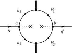
Figure 17: The non-homogeneous $B^{ab}_{0}$ function.

In the definition (F), we have assumed that the statistical distribution functions are cut off in the ultra-violet. Thus, any ultra-violet divergences anticipated from the superficial degree of divergence of the integral will be those that result from the homogeneous zero-temperature contribution. As a result, the dimensional regularization of the integral has been restricted to the $k_{1}$ dependence only.

In order to deal with the product of time-dependent energy-non-conserving vertices, we make the following replacement:

$$\delta_{t}(x)\delta_{t}(y)\ =\ \!\int_{\sigma-i\infty}^{\sigma+i\infty}\!\!\frac{\mathrm{d}{s}}{2\pi i}\;e^{st}\,\frac{2}{\pi^{2}}\,\frac{4s}{(x\>-\>y)^{2}\>+\>4s^{2}}\,\frac{1}{(x\>+\>y)^{2}\>+\>4s^{2}}\;,$$ (388)

where the RHS is the inverse Laplace transform and $s\>\in\>\mathbb{C}$ is a complex variable. The Bromwich contour is chosen so that $\sigma\>\in\>\mathbb{R}$ is larger than the real part of the right-most pole in the integrand, in order to ensure convergence. We then introduce the representation $B^{ab}_{0}(q_{1},q_{2},m_{1},m_{2},s)$ of the non-homogeneous CTP $B_{0}$ function through

$$B^{ab}(q_{1},q_{2},m_{1},m_{2},\tilde{t}_{f};\tilde{t}_{i})\ =\ \int_{\sigma-i\infty}^{\sigma+i\infty}\!\!\frac{\mathrm{d}{s}}{2\pi i}\;e^{st}\,B^{ab}_{0}(q_{1},q_{2},m_{1},m_{2},s)\;.$$ (389)

Note that $B^{ab}_{0}(q_{1},q_{2},m_{1},m_{2},s)$ is not the exact Laplace transform of $B^{ab}_{0}(q_{1},q_{2},m_{1},m_{2},t)$, since we have not transformed the $t$ dependence of the distribution functions. We suppress the dependence of $B^{ab}_{0}(q_{1},q_{2},m_{1},m_{2},s)$ on $\tilde{t}_{f}$ and $\tilde{t}_{i}$ for notational convenience.

After making the replacement (388) in (F), we obtain the integral

$$B^{ab}_{0}(q_{1},q_{2},m_{1},m_{2},s)\ =\ 8(2\pi\mu)^{4-d}e^{i(q_{1}^{0}\>-\>q_{2}^{0})\tilde{t}_{f}}\!\idotsint\!\frac{\mathrm{d}^{d}{k_{1}}}{i\pi^{2}}\,\frac{\mathrm{d}^{4}{k_{1}^{\prime}}}{(2\pi)^{4}}\,\frac{\mathrm{d}^{4}{k_{2}}}{(2\pi)^{4}}\,\frac{\mathrm{d}^{4}{k_{2}^{\prime}}}{(2\pi)^{4}}$$

$$\qquad\times\>(2\pi)^{3}\delta^{(3)}(\mathbf{q}_{1}\>-\>\mathbf{k}_{1}\>-\>\mathbf{k}_{2})(2\pi)^{3}\delta^{(3)}(\mathbf{q}_{2}\>-\>\mathbf{k}_{1}^{\prime}\>-\>\mathbf{k}_{2}^{\prime})$$

$$\qquad\times\>4s\Big{[}\Big{(}\,q_{1}^{0}\>-\>q_{2}^{0}\>-\>k_{1}^{0}\>+\>{k_{1}^{\prime}}^{0}\>-\>k_{2}^{0}\>+\>{k_{2}^{\prime}}^{0}\,\Big{)}^{2}\>+\>4s^{2}\,\Big{]}^{-1}\Big{[}\Big{(}\,q_{1}^{0}\>+\>q_{2}^{0}\>-\>k_{1}^{0}\>-\>{k_{1}^{\prime}}^{0}\>-\>k_{2}^{0}\>-\>{k_{2}^{\prime}}^{0}\,\Big{)}^{2}\>+\>4s^{2}\,\Big{]}^{-1}$$

$$\qquad\times\>\eta^{acd}\Delta^{0}_{ce}(k_{1},k_{1}^{\prime},m_{1},\tilde{t}_{f};\tilde{t}_{i})\Delta^{0,\,C}_{df}(k_{2},k_{2}^{\prime},m_{2},\tilde{t}_{f};\tilde{t}_{i})\eta^{efb}\;,$$ (390)

in which the analytic structure of the product of formerly $t$-dependent vertex functions is now manifest.

For conciseness, throughout this appendix we use the short-hand notation:

$$\sum_{\{\alpha\}}$$ (391)

for summation over only the $\alpha_{i}\>=\>\pm 1$ and $\alpha_{i}^{\prime}\>=\>\pm 1$ that appear explicitly in an expression. On-shell energies are denoted by

$$E_{i}\>\equiv\>E_{i}(\mathbf{k}_{i})\>=\>\sqrt{\mathbf{k}_{i}^{2}+m_{i}^{2}}\;,\qquad E_{i}^{\prime}\>\equiv\>E_{i}^{\prime}(\mathbf{k}_{i}^{\prime})\>=\>\sqrt{{\mathbf{k}_{i}^{\prime}}^{2}+m_{i}^{2}}\;,$$ (392)

and on-shell four-momenta by

$$\hat{k}_{i}\ \equiv\ \hat{k}^{\mu}_{i}\ =\ (\alpha_{i}E_{i}(\mathbf{k}_{i}),\mathbf{k}_{i})\;,\qquad\hat{k}_{i}^{\prime}\ \equiv\ {\hat{k}_{i}^{\prime}}{}^{\mu}\ =\ (\alpha_{i}^{\prime}E_{i}^{\prime}(\mathbf{k}_{i}^{\prime}),\mathbf{k}_{i}^{\prime})\;.$$ (393)

For the energy factor in (144), we use the notation

$$\mathscr{E}_{i}\ \equiv\ \mathscr{E}_{i}(\mathbf{k}_{i},\mathbf{k}_{i}^{\prime})\ =\ \sqrt{E_{i}(\mathbf{k}_{i})E_{i}(\mathbf{k}_{i}^{\prime})}\;.$$ (394)

Products of unit-step functions are denoted by

$$\theta(x,y,\cdots,z)\ \equiv\ \theta(x)\theta(y)\cdots\theta(z)\;.$$ (395)

Time-Ordered Functions

The $(a,b)\>=\>(1,1)$ element of (F) coincides with the time-ordered function $B_{0}$, which we may separate into four contributions (suppressing all arguments):

$$B_{0}\ =\ I^{(\mathrm{i})}\>+\>I^{(\mathrm{ii})}\>+\>I^{(\mathrm{iiia})}\>+\>I^{(\mathrm{iiib})}\;.$$ (396)

These four contributions are the zero temperature limit ($I^{(i)}$), the purely thermal term ($I^{(ii)}$) and the cross terms ($I^{(iiia)}$ and $I^{(iiib)}$).

(i) The zero-temperature part may be extracted from the product of terms that remain in the limit of vanishing statistical distribution functions. This part is

$$I^{(\mathrm{i})}(q_{1},q_{2},m_{1},m_{2},s)\ =\ 8(2\pi\mu)^{4-d}e^{i(q_{1}^{0}\>-\>q_{2}^{0})\tilde{t}_{f}}\!\idotsint\!\frac{\mathrm{d}^{d}{k_{1}}}{i\pi^{2}}\,\frac{\mathrm{d}^{4}{k_{1}^{\prime}}}{(2\pi)^{4}}\,\frac{\mathrm{d}^{4}{k_{2}}}{(2\pi)^{4}}\,\frac{\mathrm{d}^{4}{k_{2}^{\prime}}}{(2\pi)^{4}}$$

$$\qquad\times\>(2\pi)^{3}\delta^{(3)}(\mathbf{q}_{1}\>-\>\mathbf{k}_{1}\>-\>\mathbf{k}_{2})(2\pi)^{3}\delta^{(3)}(\mathbf{q}_{2}\>-\>\mathbf{k}_{1}^{\prime}\>-\>\mathbf{k}_{2}^{\prime})$$

$$\qquad\times\ 4s\Big{[}\Big{(}\,q_{1}^{0}\>-\>q_{2}^{0}\>-\>k_{1}^{0}\>+\>{k_{1}^{\prime}}^{0}\>-\>k_{2}^{0}\>+\>{k_{2}^{\prime}}^{0}\,\Big{)}^{2}\>+\>4s^{2}\,\Big{]}^{-1}\Big{[}\Big{(}\,q_{1}^{0}\>+\>q_{2}^{0}\>-\>k_{1}^{0}\>-\>{k_{1}^{\prime}}^{0}\>-\>k_{2}^{0}\>-\>{k_{2}^{\prime}}^{0}\,\Big{)}^{2}\>+\>4s^{2}\,\Big{]}^{-1}$$

$$\qquad\times\ \frac{1}{k_{1}^{2}\>-\>m_{1}^{2}\>+\>i\epsilon}(2\pi)^{4}\delta^{(4)}(k_{1}\>-\>k_{1}^{\prime})\frac{1}{k_{2}^{2}\>-\>m_{2}^{2}\>+\>i\epsilon}(2\pi)^{4}\delta^{(4)}(k_{2}\>-\>k_{2}^{\prime})\;.$$ (397)

The ${k_{1}^{\prime}}^{0}$ and ${k_{2}^{\prime}}^{0}$ integrations are performed by means of the delta functions, giving

$$I^{(\mathrm{i})}(q_{1},q_{2},m_{1},m_{2},s)\ =\ (2\pi\mu)^{4-d}e^{i(q_{1}^{0}\>-\>q_{2}^{0})\tilde{t}_{f}}\!\idotsint\!\frac{\mathrm{d}^{d-1}{k_{1}}}{i\pi^{2}}\,\frac{\mathrm{d}^{3}{\mathbf{k}_{1}^{\prime}}}{(2\pi)^{3}}\,\frac{\mathrm{d}^{3}{\mathbf{k}_{2}}}{(2\pi)^{3}}\,\frac{\mathrm{d}^{3}{\mathbf{k}_{2}^{\prime}}}{(2\pi)^{3}}\,\mathrm{d}{k_{1}^{0}}\,\mathrm{d}{k_{2}^{0}}$$

$$\qquad\times\>(2\pi)^{3}\delta^{(3)}(\mathbf{q}_{1}\>-\>\mathbf{k}_{1}\>-\>\mathbf{k}_{2})(2\pi)^{3}\delta^{(3)}(\mathbf{q}_{2}\>-\>\mathbf{k}_{1}^{\prime}\>-\>\mathbf{k}_{2}^{\prime})$$

$$\qquad\times\>\frac{4s}{\pi}\Big{[}\Big{(}\,q_{1}^{0}\>-\>q_{2}^{0}\Big{)}^{2}\>+\>4s^{2}\,\Big{]}^{-1}\Big{[}\Big{(}\tfrac{q_{1}^{0}\>+\>q_{2}^{0}}{2}\>-\>k_{1}^{0}\>-\>k_{2}^{0}\,\Big{)}^{2}\>+\>s^{2}\,\Big{]}^{-1}$$

$$\qquad\times\>\frac{1}{(k_{1}^{0})^{2}\>-\>E_{1}^{2}\>+\>i\epsilon}\,\frac{1}{(k_{2}^{0})^{2}\>-\>E_{2}^{2}\>+\>i\epsilon}(2\pi)^{3}\delta^{(3)}(\mathbf{k}_{1}\>-\>\mathbf{k}_{1}^{\prime})(2\pi)^{3}\delta^{(3)}(\mathbf{k}_{2}\>-\>\mathbf{k}_{2}^{\prime})\;.$$ (398)

By virtue of the residue theorem, we may perform the $k_{1}^{0}$ and $k_{2}^{0}$ integrations by closing contours in the lower halves of the $k_{1}^{0}$ and $k_{2}^{0}$ complex planes. After collecting together the resulting terms, we find

$$I^{(\mathrm{i})}(q_{1},q_{2},m_{1},m_{2},s)\ =\ -2(2\pi)^{3}\mu^{4-d}e^{i(q_{1}^{0}\>-\>q_{2}^{0})\tilde{t}_{f}}\sum_{\{\alpha\}}\idotsint\!\frac{\mathrm{d}^{d-1}{\mathbf{k}_{1}}}{(2\pi)^{d-1}}\,\frac{\mathrm{d}^{3}{\mathbf{k}_{1}^{\prime}}}{(2\pi)^{3}}\,\frac{\mathrm{d}^{3}{\mathbf{k}_{2}}}{(2\pi)^{3}}\,\frac{\mathrm{d}^{3}{\mathbf{k}_{2}^{\prime}}}{(2\pi)^{3}}$$

$$\qquad\times\>\frac{1}{E_{1}E_{2}}\,(2\pi)^{3}\delta^{(3)}(\mathbf{q}_{1}\>-\>\mathbf{k}_{1}\>-\>\mathbf{k}_{2})(2\pi)^{3}\delta^{(3)}(\mathbf{q}_{2}\>-\>\mathbf{k}_{1}^{\prime}\>-\>\mathbf{k}_{2}^{\prime})$$

$$\qquad\times\>\frac{1}{\pi}\Big{[}\Big{(}\,q_{1}^{0}\>-\>q_{2}^{0}\,\Big{)}^{2}\>+\>4s^{2}\,\Big{]}^{-1}\,\alpha_{1}\,\Big{[}\,\tfrac{q_{1}^{0}\>+\>q_{2}^{0}}{2}\>-\>\alpha_{1}\Big{(}\,E_{1}\>+\>E_{2}\>-\>is\,\Big{)}\Big{]}^{-1}$$

$$\qquad\times\>(2\pi)^{3}\delta^{(3)}(\mathbf{k}_{1}\>-\>\mathbf{k}_{1}^{\prime})(2\pi)^{3}\delta^{(3)}(\mathbf{k}_{2}\>-\>\mathbf{k}_{2}^{\prime})\;,$$ (399)

or, in terms of the Lorentz-invariant phase-space measures in (3),

$$I^{(\mathrm{i})}(q_{1},q_{2},m_{1},m_{2},s)\ =\ -8(2\pi)^{3}\mu^{4-d}e^{i(q_{1}^{0}\>-\>q_{2}^{0})\tilde{t}_{f}}\sum_{\{\alpha\}}\idotsint\mathrm{d}{\Pi^{d-1}_{\mathbf{k}_{1}}}\,\mathrm{d}{\Pi_{\mathbf{k}_{1}^{\prime}}}\,\mathrm{d}{\Pi_{\mathbf{k}_{2}}}\,\mathrm{d}{\Pi_{\mathbf{k}_{2}^{\prime}}}\,$$

$$\qquad\times\>(2\pi)^{3}\delta^{(3)}(\mathbf{q}_{1}\>-\>\mathbf{k}_{1}\>-\>\mathbf{k}_{2})(2\pi)^{3}\delta^{(3)}(\mathbf{q}_{2}\>-\>\mathbf{k}_{1}^{\prime}\>-\>\mathbf{k}_{2}^{\prime})$$

$$\qquad\times\>\frac{1}{\pi}\Big{[}\Big{(}\,q_{1}^{0}\>-\>q_{2}^{0}\,\Big{)}^{2}\>+\>4s^{2}\,\Big{]}^{-1}\,\alpha_{1}\,\Big{[}\,\tfrac{q_{1}^{0}\>+\>q_{2}^{0}}{2}\>-\>\alpha_{1}\Big{(}\,E_{1}\>+\>E_{2}\>-\>is\,\Big{)}\Big{]}^{-1}$$

$$\qquad\times\>(2\pi)^{3}2E_{1}^{\prime}\delta^{(3)}(\mathbf{k}_{1}\>-\>\mathbf{k}_{1}^{\prime})(2\pi)^{3}2E_{2}^{\prime}\delta^{(3)}(\mathbf{k}_{2}\>-\>\mathbf{k}_{2}^{\prime})\;,$$ (400)

where the superscript $d-1$ indicates that the $\mathbf{k}_{1}$ integration is to be taken over a $(d-1)$-dimensional phase space.

The Laplace transform $\mathcal{F}(s)$ of a complex-valued function $F(t)$ has the following properties:

$$\mathcal{L}_{t}[\mathrm{Re}\,F](s) \ =\ \frac{1}{2}\Big{[}\,\mathcal{F}(s)\>+\>\Big{(}\mathcal{F}(s^{*})\Big{)}^{*}\,\Big{]}\;,$$ (401a)

$$\mathcal{L}_{t}[\mathrm{Im}\,F](s) \ =\ \frac{1}{2i}\Big{[}\,\mathcal{F}(s)\>-\>\Big{(}\mathcal{F}(s^{*})\Big{)}^{*}\,\Big{]}\;.$$ (401b)

We may then identify the dispersive and absorptive parts of the $t$-dependent $B_{0}$ function with the parts symmetric and anti-symmetric in $s$, respectively. With this separation, (F) becomes

$$I^{(\mathrm{i})}(q_{1},q_{2},m_{1},m_{2},s)\ =\ 8(2\pi)^{3}\mu^{4-d}e^{i(q_{1}^{0}\>-\>q_{2}^{0})\tilde{t}_{f}}\sum_{\{\alpha\}}\idotsint\!\mathrm{d}{\Pi^{d-1}_{k_{1}}}\,\mathrm{d}{\Pi_{\mathbf{k}_{1}^{\prime}}}\,\mathrm{d}{\Pi_{\mathbf{k}_{2}}}\,\mathrm{d}{\Pi_{\mathbf{k}_{2}^{\prime}}}$$

$$\qquad\times\>(2\pi)^{3}\delta^{(3)}(\mathbf{q}_{1}\>-\>\mathbf{k}_{1}\>-\>\mathbf{k}_{2})(2\pi)^{3}\delta^{(3)}(\mathbf{q}_{2}\>-\>\mathbf{k}_{1}^{\prime}\>-\>\mathbf{k}_{2}^{\prime})$$

$$\qquad\times\>\frac{1}{\pi}\Big{[}\Big{(}\,q_{1}^{0}\>-\>q_{2}^{0}\,\Big{)}^{2}\>+\>4s^{2}\,\Big{]}^{-1}\,\Big{\{}\Big{[}\,\tfrac{q_{1}^{0}\>+\>q_{2}^{0}}{2}\>-\>\alpha_{1}\Big{(}\,E_{1}\>+\>E_{2}\,\Big{)}\Big{]}^{2}\>+\>s^{2}\,\Big{\}}^{-1}$$

$$\qquad\times\>\Big{\{}\,-\alpha_{1}\Big{[}\,\tfrac{q_{1}^{0}\>+\>q_{2}^{0}}{2}\>-\>\alpha_{1}\Big{(}\,E_{1}\>+\>E_{2}\,\Big{)}\Big{]}\>+\>is\,\Big{\}}(2\pi)^{3}2E_{1}^{\prime}\delta^{(3)}(\mathbf{k}_{1}\>-\>\mathbf{k}_{1}^{\prime})(2\pi)^{3}2E_{2}^{\prime}\delta^{(3)}(\mathbf{k}_{2}\>-\>\mathbf{k}_{2}^{\prime})\;,$$ (402)

where the delineation between dispersive and absorptive parts is identified in the second set of curly brackets.

Isolating the dispersive part of this result and performing all but one of the remaining phase-space integrals, we find

$$\mathrm{Disp}\,I^{(\mathrm{i})}(q_{1},q_{2},m_{1},m_{2},s)\ =\ (2\pi)^{4}\frac{1}{\pi}\,\frac{1}{\big{(}\,q_{1}^{0}\>-\>q_{2}^{0}\,\big{)}^{2}\>+\>4s^{2}}\delta^{(3)}(\mathbf{q}_{1}\>-\>\mathbf{q}_{2})e^{i(q_{1}^{0}\>-\>q_{2}^{0})\tilde{t}_{f}}$$

$$\qquad\times\sum_{\{\alpha\}}\Big{\{}-(2\pi\mu)^{4-d}\!\int\!\mathrm{d}^{d-1}{\mathbf{k}_{1}}\,\frac{E_{1}\>+\>E_{2}}{E_{1}E_{2}}\,\frac{1}{\pi}\Big{[}\Big{(}\,\tfrac{q_{1}^{0}+q_{2}^{0}}{2}\>-\>i\alpha s\,\Big{)}^{2}\>-\>\Big{(}\,E_{1}\>+\>E_{2}\,\Big{)}^{2}\,\Big{]}^{-1}\Big{\}}\;,$$ (403)

where $\mathrm{Disp}$ stands for the dispersive part. We compare this result to the form of the zero-temperature $B_{0}$ function (385) after the $k_{0}$ integration has been performed:

$$B_{0}^{T\>=\>0}(q,m_{1},m_{2})\ =\ -(2\pi\mu)^{4-d}\!\int\!\mathrm{d}^{d-1}{\mathbf{k}_{1}}\;\frac{E_{1}\>+\>E_{2}}{E_{1}E_{2}}\,\frac{1}{\pi}\,\Big{[}\,q^{2}_{0}\>-\>\Big{(}\,E_{1}\>+\>E_{2}\,\Big{)}^{2}\,\Big{]}^{-1}\;.$$ (404)

Hence, we may write

$$\mathrm{Disp}\,I^{(\mathrm{i})}(q_{1},q_{2},m_{1},m_{2},s)\ =\ (2\pi)^{4}\frac{1}{\pi}\,\frac{1}{\big{(}\,q_{1}^{0}\>-\>q_{2}^{0}\,\big{)}^{2}\>+\>4s^{2}}\delta^{(3)}(\mathbf{q}_{1}\>-\>\mathbf{q}_{2})e^{i(q_{1}^{0}\>-\>q_{2}^{0})\tilde{t}_{f}}$$

$$\qquad\times\>\sum_{\{\alpha\}}B^{T\>=\>0}_{0}\Big{(}\tfrac{q_{1}^{0}+q_{2}^{0}}{2}-i\alpha s,\tfrac{\mathbf{q}_{1}+\mathbf{q}_{2}}{2},m_{1},m_{2}\Big{)}\;,$$ (405)

where, for $d\>=\>4\>-\>2\epsilon$ dimensions,

$$B^{T=0}_{0}(q^{0}-i\alpha s,\mathbf{q},m_{1},m_{2})\ =\ \frac{1}{\epsilon}\>-\>\gamma_{\mathrm{E}}\>+\>\ln\frac{4\pi\mu^{2}}{m_{1}m_{2}}\ +\ \frac{1}{\big{(}q^{0}\>-\>i\alpha s\big{)}^{2}\>-\>\mathbf{q}^{2}}\bigg{[}\,\big{(}m_{2}^{2}\>-\>m_{1}^{2}\big{)}\ln\frac{m_{1}^{2}}{m_{2}^{2}}$$

$$\qquad+\>\lambda^{1/2}\big{(}(q^{0}-i\alpha s)^{2}-\mathbf{q}^{2},m_{1}^{2},m_{2}^{2}\big{)}\cosh^{-1}\bigg{(}\,\frac{m_{1}^{2}\>+\>m_{2}^{2}\>-\>(q^{0}-i\alpha s)^{2}\>+\>\mathbf{q}^{2}}{2m_{1}m_{2}}\,\bigg{)}\bigg{]}\;,$$ (406)

containing the zero-temperature UV divergence ’t Hooft and Veltman (1979). In (F), $\gamma_{\mathrm{E}}$ is the Euler constant and $\mu$ is the ’t Hooft mass scale.

(ii) The purely thermal part is more straightforward to analyze:

$$I^{(\mathrm{ii})}(q_{1},q_{2},m_{1},m_{2},s)\ =\ -8(2\pi\mu)^{4-d}e^{i(q_{1}^{0}\>-\>q_{2}^{0})\tilde{t}_{f}}\!\idotsint\!\frac{\mathrm{d}^{d}{k_{1}}}{i\pi^{2}}\,\frac{\mathrm{d}^{4}{k_{1}^{\prime}}}{(2\pi)^{4}}\,\frac{\mathrm{d}^{4}{k_{2}}}{(2\pi)^{4}}\,\frac{\mathrm{d}^{4}{k_{2}^{\prime}}}{(2\pi)^{4}}$$

$$\qquad\times\>(2\pi)^{3}\delta^{(3)}(\mathbf{q}_{1}\>-\>\mathbf{k}_{1}\>-\>\mathbf{k}_{2})(2\pi)^{3}\delta^{(3)}(\mathbf{q}_{2}\>-\>\mathbf{k}_{1}^{\prime}\>-\>\mathbf{k}_{2}^{\prime})$$

$$\qquad\times\>4s\Big{[}\Big{(}\,q_{1}^{0}\>-\>q_{2}^{0}\>-\>k_{1}^{0}\>+\>{k_{1}^{\prime}}^{0}\>-\>k_{2}^{0}\>+\>{k_{2}^{\prime}}^{0}\,\Big{)}^{2}\>+\>4s^{2}\,\Big{]}^{-1}\Big{[}\Big{(}\,q_{1}^{0}\>+\>q_{2}^{0}\>-\>k_{1}^{0}\>-\>{k_{1}^{\prime}}^{0}\>-\>k_{2}^{0}\>-\>{k_{2}^{\prime}}^{0}\,\Big{)}^{2}\>+\>4s^{2}\,\Big{]}^{-1}$$

$$\qquad\times\ 2\pi\delta(k_{1}^{2}\>-\>m_{1}^{2})|2k_{1}^{0}|^{1/2}\tilde{f}_{1}(k_{1},k_{1}^{\prime},t)e^{i(k_{1}^{0}\>-\>{k_{1}^{\prime}}^{0})\tilde{t}_{f}}|2{k_{1}^{\prime}}^{0}|^{1/2}2\pi\delta({k_{1}^{\prime}}^{2}\>-\>m_{1}^{2})$$

$$\qquad\times\ 2\pi\delta(k_{2}^{2}\>-\>m_{2}^{2})|2k_{2}^{0}|^{1/2}\tilde{f}^{C}_{2}(k_{2},k_{2}^{\prime},t)e^{i(k_{2}^{0}\>-\>{k_{2}^{\prime}}^{0})\tilde{t}_{f}}|2{k_{2}^{\prime}}^{0}|^{1/2}2\pi\delta({k_{2}^{\prime}}^{2}\>-\>m_{2}^{2})\;.$$ (407)

Performing the four zeroth-component momentum integrations by virtue of the on-shell delta functions $\delta(k_{i}^{2}\>-\>m_{i}^{2})$ and $\delta({k_{i}^{\prime}}^{2}\>-\>m_{i}^{2})$ in (F), we find

$$I^{(\mathrm{ii})}(q_{1},q_{2},m_{1},m_{2},s)\ =\ 8(2\pi)^{3}\mu^{4-d}e^{i(q_{1}^{0}\>-\>q_{2}^{0})\tilde{t}_{f}}\sum_{\{\alpha\}}\idotsint\!\mathrm{d}{\Pi^{d-1}_{k_{1}}}\,\mathrm{d}{\Pi_{\mathbf{k}_{1}^{\prime}}}\,\mathrm{d}{\Pi_{\mathbf{k}_{2}}}\,\mathrm{d}{\Pi_{\mathbf{k}_{2}^{\prime}}}$$

$$\qquad\times\>(2\pi)^{3}\delta^{(3)}(\mathbf{q}_{1}\>-\>\mathbf{k}_{1}\>-\>\mathbf{k}_{2})(2\pi)^{3}\delta^{(3)}(\mathbf{q}_{2}\>-\>\mathbf{k}_{1}^{\prime}\>-\>\mathbf{k}_{2}^{\prime})$$

$$\qquad\times\>\Big{[}\Big{(}\,q_{1}^{0}\>-\>q_{2}^{0}\>-\>\alpha_{1}E_{1}\>+\>\alpha_{1}^{\prime}E_{1}^{\prime}\>-\>\alpha_{2}E_{2}\>+\>\alpha_{2}^{\prime}E_{2}^{\prime}\,\Big{)}^{2}\>+\>4s^{2}\,\Big{]}^{-1}$$

$$\qquad\times\>\Big{[}\Big{(}\,\tfrac{q_{1}^{0}\>+\>q_{2}^{0}}{2}\>-\>\tfrac{\alpha_{1}E_{1}\>+\>\alpha_{1}^{\prime}E_{1}^{\prime}}{2}\>-\>\tfrac{\alpha_{2}E_{2}\>+\>\alpha_{2}^{\prime}E_{2}^{\prime}}{2}\,\Big{)}^{2}\>+\>s^{2}\,\Big{]}^{-1}\>2is$$

$$\qquad\times\ 2\mathscr{E}_{1}\tilde{f}_{1}(\hat{k}_{1},\hat{k}_{1}^{\prime},t)e^{i(\alpha_{1}E_{1}\>-\>\alpha_{1}^{\prime}E_{1}^{\prime})\tilde{t}_{f}}2\mathscr{E}_{2}\tilde{f}_{2}^{C}(\hat{k}_{2},\hat{k}_{2}^{\prime},t)e^{i(\alpha_{2}E_{2}\>-\>\alpha_{2}^{\prime}E_{2}^{\prime})\tilde{t}_{f}}\;.$$ (408)

Note that the purely thermal part in (F) contains only absorptive contributions.

(iii) The cross-terms yield both dispersive and absorptive contributions. The first of the cross terms yields

$$I^{(\mathrm{iiia})}(q_{1},q_{2},m_{1},m_{2},s)\ =\ -8i(2\pi\mu)^{4-d}e^{i(q_{1}^{0}\>-\>q_{2}^{0})\tilde{t}_{f}}\!\idotsint\!\frac{\mathrm{d}^{d}{k_{1}}}{i\pi^{2}}\,\frac{\mathrm{d}^{4}{k_{1}^{\prime}}}{(2\pi)^{4}}\,\frac{\mathrm{d}^{4}{k_{2}}}{(2\pi)^{4}}\,\frac{\mathrm{d}^{4}{k_{2}^{\prime}}}{(2\pi)^{4}}$$

$$\qquad\times\>(2\pi)^{3}\delta^{(3)}(\mathbf{q}_{1}\>-\>\mathbf{k}_{1}\>-\>\mathbf{k}_{2})(2\pi)^{3}\delta^{(3)}(\mathbf{q}_{2}\>-\>\mathbf{k}_{1}^{\prime}\>-\>\mathbf{k}_{2}^{\prime})$$

$$\qquad\times\ 4s\Big{[}\Big{(}\,q_{1}^{0}\>-\>q_{2}^{0}\>-\>k_{1}^{0}\>+\>{k_{1}^{\prime}}^{0}\>-\>k_{2}^{0}\>+\>{k_{2}^{\prime}}^{0}\,\Big{)}^{2}\>+\>4s^{2}\,\Big{]}^{-1}\Big{[}\Big{(}\,q_{1}^{0}\>+\>q_{2}^{0}\>-\>k_{1}^{0}\>-\>{k_{1}^{\prime}}^{0}\>-\>k_{2}^{0}\>-\>{k_{2}^{\prime}}^{0}\,\Big{)}^{2}\>+\>4s^{2}\,\Big{]}^{-1}$$

$$\qquad\times\>\frac{1}{k_{1}^{2}\>-\>m_{1}^{2}\>+\>i\epsilon}(2\pi)^{4}\delta^{(4)}(k_{1}\>-\>k_{1}^{\prime})$$

$$\qquad\times\ 2\pi\delta(k_{2}^{2}\>-\>m_{2}^{2})|2k_{2}^{0}|^{1/2}\tilde{f}_{2}^{C}(k_{2},k_{2}^{\prime},t)e^{i(k_{2}^{0}\>-\>{k_{2}^{\prime}}^{0})\tilde{t}_{f}}|2{k_{2}^{\prime}}^{0}|^{1/2}2\pi\delta({k_{2}^{\prime}}^{2}\>-\>m_{2}^{2})\;.$$ (409)

After evaluating the ${k_{1}^{\prime}}^{0}$, $k_{2}^{0}$ and ${k_{2}^{\prime}}^{0}$ integrals by virtue of the delta functions, we perform the $k_{1}^{0}$ integral by closing a contour in the lower half of the $k_{1}^{0}$ complex plane. Equation (F) may then be written in the more compact form

$$I^{(\mathrm{iiia})}(q_{1},q_{2},m_{1},m_{2},s)\ =\ -8(2\pi)^{3}\mu^{4-d}e^{i(q_{1}^{0}\>-\>q_{2}^{0})\tilde{t}_{f}}\sum_{\{\alpha\}}\idotsint\!\mathrm{d}{\Pi^{d-1}_{\mathbf{k}_{1}}}\,\mathrm{d}{\Pi_{\mathbf{k}_{1}^{\prime}}}\,\mathrm{d}{\Pi_{\mathbf{k}_{2}}}\,\mathrm{d}{\Pi_{\mathbf{k}_{2}^{\prime}}}$$

$$\qquad\times\>(2\pi)^{3}\delta^{(3)}(\mathbf{q}_{1}\>-\>\mathbf{k}_{1}\>-\>\mathbf{k}_{2})(2\pi)^{3}\delta^{(3)}(\mathbf{q}_{2}\>-\>\mathbf{k}_{1}^{\prime}\>-\>\mathbf{k}_{2}^{\prime})$$

$$\qquad\times\>\frac{1}{\pi}\Big{[}\Big{(}\,q_{1}^{0}\>-\>q_{2}^{0}\>-\>\alpha_{2}E_{2}\>+\>\alpha_{2}^{\prime}E_{2}^{\prime}\,\Big{)}^{2}\>+\>4s^{2}\,\Big{]}^{-1}\alpha_{1}\,\Big{[}\,\tfrac{q_{1}^{0}\>+\>q_{2}^{0}}{2}\>-\>\tfrac{\alpha_{2}E_{2}\>+\>\alpha_{2}^{\prime}E_{2}^{\prime}}{2}\>-\>\alpha_{1}\Big{(}\,E_{1}\>-\>is\,\Big{)}\Big{]}^{-1}$$

$$\qquad\times(2\pi)^{3}2E_{1}^{\prime}\delta^{(3)}(\mathbf{k}_{1}\>-\>\mathbf{k}_{1}^{\prime})2\mathscr{E}_{2}\tilde{f}_{2}^{C}(\hat{k}_{2},\hat{k}^{\prime}_{2},t)e^{i(\alpha_{2}E_{2}\>-\>\alpha_{2}^{\prime}E_{2}^{\prime})\tilde{t}_{f}}\;.$$ (410)

Separating again into dispersive and absorptive parts as in (F), $I^{(\mathrm{iiia})}$ may be written as

$$I^{(\mathrm{iiia})}(q_{1},q_{2},m_{1},m_{2},s)\ =\ 8(2\pi)^{3}\mu^{4-d}e^{i(q_{1}^{0}\>-\>q_{2}^{0})\tilde{t}_{f}}\sum_{\{\alpha\}}\idotsint\!\mathrm{d}{\Pi^{d-1}_{\mathbf{k}_{1}}}\,\mathrm{d}{\Pi_{\mathbf{k}_{1}^{\prime}}}\,\mathrm{d}{\Pi_{\mathbf{k}_{2}}}\,\mathrm{d}{\Pi_{\mathbf{k}_{2}^{\prime}}}$$

$$\qquad\times\>(2\pi)^{3}\delta^{(3)}(\mathbf{q}_{1}\>-\>\mathbf{k}_{1}\>-\>\mathbf{k}_{2})(2\pi)^{3}\delta^{(3)}(\mathbf{q}_{2}\>-\>\mathbf{k}_{1}^{\prime}\>-\>\mathbf{k}_{2}^{\prime})$$

$$\qquad\times\>\frac{1}{\pi}\Big{[}\Big{(}\,q_{1}^{0}\>-\>q_{2}^{0}\>-\>\alpha_{2}E_{2}\>+\>\alpha_{2}^{\prime}E_{2}^{\prime}\,\Big{)}^{2}\>+\>4s^{2}\,\Big{]}^{-1}\Big{[}\Big{(}\,\tfrac{q_{1}^{0}\>+\>q_{2}^{0}}{2}\>-\>\alpha_{1}E_{1}\>-\>\tfrac{\alpha_{2}E_{2}\>+\>\alpha_{2}^{\prime}E_{2}^{\prime}}{2}\,\Big{)}^{2}\>+\>s^{2}\,\Big{]}^{-1}$$

$$\qquad\times\ \Big{\{}\,-\alpha_{1}\Big{(}\,\tfrac{q_{1}^{0}\>+\>q_{2}^{0}}{2}\>-\>\alpha_{1}E_{1}\>-\>\tfrac{\alpha_{2}E_{2}\>+\>\alpha_{2}^{\prime}E_{2}^{\prime}}{2}\,\Big{)}\>+\>is\,\Big{\}}$$

$$\qquad\times\ (2\pi)^{3}2E_{1}^{\prime}\delta^{(3)}(\mathbf{k}_{1}\>-\>\mathbf{k}_{1}^{\prime})2\mathscr{E}_{1}\tilde{f}_{2}^{C}(\hat{k}_{2},\hat{k}_{2}^{\prime},t)e^{i(\alpha_{2}E_{2}\>-\>\alpha_{2}^{\prime}E_{2}^{\prime})\tilde{t}_{f}}\;.$$ (411)

Similarly, for the second cross term $I^{(\mathrm{iiib})}$ in (396) , we obtain

$$I^{(\mathrm{iiib})}(q_{1},q_{2},m_{1},m_{2},s)\ =\ 8(2\pi)^{3}\mu^{4-d}e^{i(q_{1}^{0}\>-\>q_{2}^{0})\tilde{t}_{f}}\sum_{\{\alpha\}}\idotsint\!\mathrm{d}{\Pi^{d-1}_{\mathbf{k}_{1}}}\,\mathrm{d}{\Pi_{\mathbf{k}_{1}^{\prime}}}\,\mathrm{d}{\Pi_{\mathbf{k}_{2}}}\,\mathrm{d}{\Pi_{\mathbf{k}_{2}^{\prime}}}$$

$$\qquad\times\>(2\pi)^{3}\delta^{(3)}(\mathbf{q}_{1}\>-\>\mathbf{k}_{1}\>-\>\mathbf{k}_{2})(2\pi)^{3}\delta^{(3)}(\mathbf{q}_{2}\>-\>\mathbf{k}_{1}^{\prime}\>-\>\mathbf{k}_{2}^{\prime})$$

$$\qquad\times\>\frac{1}{\pi}\Big{[}\Big{(}\,q_{1}^{0}\>-\>q_{2}^{0}\>-\>\alpha_{1}E_{1}\>+\>\alpha_{1}^{\prime}E_{1}^{\prime}\,\Big{)}^{2}\>+\>4s^{2}\,\Big{]}^{-1}\Big{[}\Big{(}\,\tfrac{q_{1}^{0}\>+\>q_{2}^{0}}{2}\>-\>\tfrac{\alpha_{1}E_{1}\>+\>\alpha_{1}^{\prime}E_{1}^{\prime}}{2}\>-\>\alpha_{2}E_{2}\,\Big{)}^{2}\>+\>s^{2}\,\Big{]}^{-1}$$

$$\qquad\times\>\Big{\{}\,-\alpha_{2}\Big{(}\,\tfrac{q_{1}^{0}\>+\>q_{2}^{0}}{2}\>-\>\tfrac{\alpha_{1}E_{1}\>+\>\alpha_{1}^{\prime}E_{1}^{\prime}}{2}\>-\>\alpha_{2}E_{2}\,\Big{)}\>+\>is\,\Big{\}}$$

$$\qquad\times\ (2\pi)^{3}2E_{2}^{\prime}\delta^{(3)}(\mathbf{k}_{2}\>-\>\mathbf{k}_{2}^{\prime})2\mathscr{E}_{1}\tilde{f}_{1}(\hat{k}_{1},\hat{k}_{1}^{\prime},t)e^{i(\alpha_{1}E_{1}\>-\>\alpha_{1}^{\prime}E_{1}^{\prime})\tilde{t}_{f}}\;.$$ (412)

Collecting the four contributions from (F), (F), (F) and (F) together, we find the full time-ordered function

$$B_{0}(q_{1},q_{2},m_{1},m_{2},s)\ =\ 8(2\pi)^{3}\mu^{4-d}e^{i(q_{1}^{0}\>-\>q_{2}^{0})\tilde{t}_{f}}\sum_{\{\alpha\}}\idotsint\!\mathrm{d}{\Pi^{d-1}_{\mathbf{k}_{1}}}\,\mathrm{d}{\Pi_{\mathbf{k}_{1}^{\prime}}}\,\mathrm{d}{\Pi_{\mathbf{k}_{2}}}\,\mathrm{d}{\Pi_{\mathbf{k}_{2}^{\prime}}}$$

$$\qquad\times\>(2\pi)^{3}\delta^{(3)}(\mathbf{q}_{1}\>-\>\mathbf{k}_{1}\>-\>\mathbf{k}_{2})(2\pi)^{3}\delta^{(3)}(\mathbf{q}_{2}\>-\>\mathbf{k}_{1}^{\prime}\>-\>\mathbf{k}_{2}^{\prime})2\mathscr{E}_{1}e^{i(\alpha_{1}E_{1}\>-\>\alpha_{1}^{\prime}E_{1}^{\prime})\tilde{t}_{f}}2\mathscr{E}_{2}e^{i(\alpha_{2}E_{2}\>-\>\alpha_{2}^{\prime}E_{2}^{\prime})\tilde{t}_{f}}$$

$$\qquad\times\>\frac{1}{\pi}\Big{[}\Big{(}\,q_{1}^{0}\>-\>q_{2}^{0}\>-\>\alpha_{1}E_{1}\>+\>\alpha_{1}^{\prime}E_{1}^{\prime}\>-\>\alpha_{2}E_{2}\>+\>\alpha_{2}^{\prime}E_{2}^{\prime}\,\Big{)}^{2}\>+\>4s^{2}\,\Big{]}^{-1}$$

$$\qquad\times\ \Big{[}\Big{(}\,\tfrac{q_{1}^{0}\>+\>q_{2}^{0}}{2}\>-\>\tfrac{\alpha_{1}E_{1}\>+\>\alpha_{1}^{\prime}E_{1}^{\prime}}{2}\>-\>\tfrac{\alpha_{2}E_{2}\>+\>\alpha_{2}^{\prime}E_{2}^{\prime}}{2}\,\Big{)}^{2}\>+\>s^{2}\,\Big{]}^{-1}$$

$$\qquad\times\>\Big{\{}\,-\Big{(}\,\tfrac{q_{1}^{0}\>+\>q_{2}^{0}}{2}\>-\>\tfrac{\alpha_{1}E_{1}\>+\>\alpha_{1}^{\prime}E_{1}^{\prime}}{2}\>-\>\tfrac{\alpha_{2}E_{2}\>+\>\alpha_{2}^{\prime}E_{2}^{\prime}}{2}\,\Big{)}F^{\mathrm{R}}(\{\hat{k}\},t)\>+\>isF^{1}(\{\hat{k}\},t)\,\Big{\}}\;,$$ (413)

where $\{\hat{k}\}\>\equiv\>\{\hat{k}_{1},\hat{k}_{1}^{\prime},\hat{k}_{2},\hat{k}_{2}^{\prime}\}$ is the set of on-shell four momenta. The statistical structure is contained within the distributions $F^{\mathrm{R}}(\{\hat{k}\},t)$ and $F^{1}(\{\hat{k}\},t)$ defined as follows:

$$F^{\mathrm{R}}(\{\hat{k}\},t)\ =\ (2\pi)^{3}\delta^{(3)}(\mathbf{k}_{1}\>-\>\mathbf{k}_{1}^{\prime})(2\pi)^{3}\delta^{(3)}(\mathbf{k}_{2}\>-\>\mathbf{k}_{2}^{\prime})\Big{(}\,\theta(\alpha_{1},\alpha_{1}^{\prime},\alpha_{2},\alpha_{2}^{\prime})\>-\>\theta(-\alpha_{1},-\alpha_{1}^{\prime},-\alpha_{2},-\alpha_{2}^{\prime})\,\Big{)}$$

$$\qquad+\>(2\pi)^{3}\delta^{(3)}(\mathbf{k}_{1}\>-\>\mathbf{k}_{1}^{\prime})\Big{(}\,\theta(\alpha_{1},\alpha_{1}^{\prime})\>-\>\theta(-\alpha_{1},-\alpha_{1}^{\prime})\,\Big{)}\tilde{f}_{2}^{C}(\hat{k}_{2},\hat{k}_{2}^{\prime},t)$$

$$\qquad+\>\tilde{f}_{1}(\hat{k}_{1},\hat{k}_{1}^{\prime},t)(2\pi)^{3}\delta^{(3)}(\mathbf{k}_{2}\>-\>\mathbf{k}_{2}^{\prime})\Big{(}\,\theta(\alpha_{2},\alpha_{2}^{\prime})\>-\>\theta(-\alpha_{2},-\alpha_{2}^{\prime})\,\Big{)}\;,$$ (414a)

$$F^{1}(\{\hat{k}\},t)\ =\ (2\pi)^{3}\delta^{(3)}(\mathbf{k}_{1}\>-\>\mathbf{k}_{1}^{\prime})(2\pi)^{3}\delta^{(3)}(\mathbf{k}_{2}\>-\>\mathbf{k}_{2}^{\prime})\Big{(}\,\theta(\alpha_{1},\alpha_{1}^{\prime},\alpha_{2},\alpha_{2}^{\prime})\>+\>\theta(-\alpha_{1},-\alpha_{1}^{\prime},-\alpha_{2},-\alpha_{2}^{\prime})\,\Big{)}$$

$$\qquad+\>(2\pi)^{3}\delta^{(3)}(\mathbf{k}_{1}\>-\>\mathbf{k}_{1}^{\prime})\Big{(}\,\theta(\alpha_{1},\alpha_{1}^{\prime})\>+\>\theta(-\alpha_{1},-\alpha_{1}^{\prime})\,\Big{)}\tilde{f}_{2}^{C}(\hat{k}_{2},\hat{k}_{2}^{\prime},t)$$

$$\qquad+\>\tilde{f}_{1}(\hat{k}_{1},\hat{k}_{1}^{\prime},t)(2\pi)^{3}\delta^{(3)}(\mathbf{k}_{2}\>-\>\mathbf{k}_{2}^{\prime})\Big{(}\,\theta(\alpha_{2},\alpha_{2}^{\prime})\>+\>\theta(-\alpha_{2},-\alpha_{2}^{\prime})\,\Big{)}\>+\>2\tilde{f}_{1}(\hat{k}_{1},\hat{k}_{1}^{\prime},t)\tilde{f}^{C}_{2}(\hat{k}_{2},\hat{k}_{2}^{\prime},t)\;.$$ (414b)

For completeness, the anti-time-ordered function, obtained from the RHS of (F) by taking $s\to-s$ and multiplying by an overall minus sign, is given by

$$-B_{0}^{*}(q_{1},q_{2},m_{1},m_{2},s)\ =\ 8(2\pi)^{3}\mu^{4-d}e^{i(q_{1}^{0}\>-\>q_{2}^{0})\tilde{t}_{f}}\sum_{\{\alpha\}}\idotsint\!\mathrm{d}{\Pi^{d-1}_{\mathbf{k}_{1}}}\,\mathrm{d}{\Pi_{\mathbf{k}_{1}^{\prime}}}\,\mathrm{d}{\Pi_{\mathbf{k}_{2}}}\,\mathrm{d}{\Pi_{\mathbf{k}_{2}^{\prime}}}$$

$$\qquad\times\>(2\pi)^{3}\delta^{(3)}(\mathbf{q}_{1}\>-\>\mathbf{k}_{1}\>-\>\mathbf{k}_{2})(2\pi)^{3}\delta^{(3)}(\mathbf{q}_{2}\>-\>\mathbf{k}_{1}^{\prime}\>-\>\mathbf{k}_{2}^{\prime})2\mathscr{E}_{1}e^{i(\alpha_{1}E_{1}\>-\>\alpha_{1}^{\prime}E_{1}^{\prime})\tilde{t}_{f}}2\mathscr{E}_{2}e^{i(\alpha_{2}E_{2}\>-\>\alpha_{2}^{\prime}E_{2}^{\prime})\tilde{t}_{f}}$$

$$\qquad\times\ \frac{1}{\pi}\Big{[}\Big{(}\,q_{1}^{0}\>-\>q_{2}^{0}\>-\>\alpha_{1}E_{1}\>+\>\alpha_{1}^{\prime}E_{1}^{\prime}\>-\>\alpha_{2}E_{2}\>+\>\alpha_{2}^{\prime}E_{2}^{\prime}\,\Big{)}^{2}\>+\>4s^{2}\,\Big{]}^{-1}$$

$$\qquad\times\ \Big{[}\Big{(}\,\tfrac{q_{1}^{0}\>+\>q_{2}^{0}}{2}\>-\>\tfrac{\alpha_{1}E_{1}\>+\>\alpha_{1}^{\prime}E_{1}^{\prime}}{2}\>-\>\tfrac{\alpha_{2}E_{2}\>+\>\alpha_{2}^{\prime}E_{2}^{\prime}}{2}\,\Big{)}^{2}\>+\>s^{2}\,\Big{]}^{-1}$$

$$\qquad\times\ \Big{\{}\,\Big{(}\,\tfrac{q_{1}^{0}\>+\>q_{2}^{0}}{2}\>-\>\tfrac{\alpha_{1}E_{1}\>+\>\alpha_{1}^{\prime}E_{1}^{\prime}}{2}\>-\>\tfrac{\alpha_{2}E_{2}\>+\>\alpha_{2}^{\prime}E_{2}^{\prime}}{2}\,\Big{)}F^{\mathrm{R}}(\{\hat{k}\},t)\>+\>isF^{1}(\{\hat{k}\},t)\,\Big{\}}\;,$$ (415)

Finally, from (117a), the ‘Hadamard’ function $B_{0}^{1}$ is given by

$$B^{1}_{0}(q_{1},q_{2},m_{1},m_{2},s)\ =\ 16(2\pi)^{3}\mu^{4-d}e^{i(q_{1}^{0}\>-\>q_{2}^{0})\tilde{t}_{f}}\sum_{\{\alpha\}}\idotsint\!\mathrm{d}{\Pi^{d-1}_{\mathbf{k}_{1}}}\,\mathrm{d}{\Pi_{\mathbf{k}_{1}^{\prime}}}\,\mathrm{d}{\Pi_{\mathbf{k}_{2}}}\,\mathrm{d}{\Pi_{\mathbf{k}_{2}^{\prime}}}$$

$$\qquad\times\>(2\pi)^{3}\delta^{(3)}(\mathbf{q}_{1}\>-\>\mathbf{k}_{1}\>-\>\mathbf{k}_{2})(2\pi)^{3}\delta^{(3)}(\mathbf{q}_{2}\>-\>\mathbf{k}_{1}^{\prime}\>-\>\mathbf{k}_{2}^{\prime})2\mathscr{E}_{1}e^{i(\alpha_{1}E_{1}\>-\>\alpha_{1}^{\prime}E_{1}^{\prime})\tilde{t}_{f}}2\mathscr{E}_{2}e^{i(\alpha_{2}E_{2}\>-\>\alpha_{2}^{\prime}E_{2}^{\prime})\tilde{t}_{f}}$$

$$\qquad\times\ \frac{1}{\pi}\Big{[}\Big{(}\,q_{1}^{0}\>-\>q_{2}^{0}\>-\>\alpha_{1}E_{1}\>+\>\alpha_{1}^{\prime}E_{1}^{\prime}\>-\>\alpha_{2}E_{2}\>+\>\alpha_{2}^{\prime}E_{2}^{\prime}\,\Big{)}^{2}\>+\>4s^{2}\,\Big{]}^{-1}$$

$$\qquad\times\ \Big{[}\Big{(}\,\tfrac{q_{1}^{0}\>+\>q_{2}^{0}}{2}\>-\>\tfrac{\alpha_{1}E_{1}\>+\>\alpha_{1}^{\prime}E_{1}^{\prime}}{2}\>-\>\tfrac{\alpha_{2}E_{2}\>+\>\alpha_{2}^{\prime}E_{2}^{\prime}}{2}\,\Big{)}^{2}\>+\>s^{2}\,\Big{]}^{-1}isF^{1}(\{\hat{k}\},t)\;,$$ (416)

which depends only on $F^{1}(\{\hat{k}\},t)$, as one should expect.

Absolutely-Ordered Functions

We turn our attention now to the $(a,b)\>=\>(2,1)$ and $(a,b)\>=\>(1,2)$ elements of (386). These are the positive- and negative-frequency absolutely-ordered functions, respectively:

$$B^{>(<)}_{0}(q_{1},q_{2},m_{1},m_{2},s)\ =\ -8(2\pi\mu)^{4-d}e^{i(q_{1}^{0}\>-\>q_{2}^{0})\tilde{t}_{f}}\!\idotsint\!\frac{\mathrm{d}^{d}{k_{1}}}{i\pi^{2}}\,\frac{\mathrm{d}^{4}{k_{1}^{\prime}}}{(2\pi)^{4}}\,\frac{\mathrm{d}^{4}{k_{2}}}{(2\pi)^{4}}\,\frac{\mathrm{d}^{4}{k_{2}^{\prime}}}{(2\pi)^{4}}$$

$$\qquad\times\>(2\pi)^{3}\delta^{(3)}(\mathbf{q}_{1}\>-\>\mathbf{k}_{1}\>-\>\mathbf{k}_{2})(2\pi)^{3}\delta^{(3)}(\mathbf{q}_{2}\>-\>\mathbf{k}_{1}^{\prime}\>-\>\mathbf{k}_{2}^{\prime})$$

$$\qquad\times\ 4s\Big{[}\Big{(}\,q_{1}^{0}\>-\>q_{2}^{0}\>-\>k_{1}^{0}\>+\>{k_{1}^{\prime}}^{0}\>-\>k_{2}^{0}\>+\>{k_{2}^{\prime}}^{0}\,\Big{)}^{2}\>+\>4s^{2}\,\Big{]}^{-1}\Big{[}\Big{(}\,q_{1}^{0}\>+\>q_{2}^{0}\>-\>k_{1}^{0}\>-\>{k_{1}^{\prime}}^{0}\>-\>k_{2}^{0}\>-\>{k_{2}^{\prime}}^{0}\,\Big{)}^{2}\>+\>4s^{2}\,\Big{]}^{-1}$$

$$\qquad\times\>2\pi\delta(k_{1}^{2}\>-\>m_{1}^{2})|2k_{1}^{0}|^{1/2}\Big{(}\,\theta((-)k_{1}^{0},(-){k_{1}^{\prime}}^{0})(2\pi)^{3}\delta^{(3)}(\mathbf{k}_{1}\>-\>\mathbf{k}_{1}^{\prime})\>+\>\tilde{f}_{1}(k_{1},k_{1}^{\prime},t)\,\Big{)}$$

$$\qquad\qquad\times\>e^{i(k_{1}^{0}\>-\>{k_{1}^{\prime}}^{0})\tilde{t}_{f}}|2{k_{1}^{\prime}}^{0}|^{1/2}2\pi\delta({k_{1}^{\prime}}^{2}\>-\>m_{1}^{2})$$

$$\qquad\times\>2\pi\delta(k_{2}^{2}\>-\>m_{2}^{2})|2k_{2}^{0}|^{1/2}\Big{(}\,\theta((-)k_{2}^{0},(-){k_{2}^{\prime}}^{0})(2\pi)^{3}\delta^{(3)}(\mathbf{k}_{2}\>-\>\mathbf{k}_{2}^{\prime})\>+\>\tilde{f}_{2}^{C}(k_{2},k_{2}^{\prime},t)\,\Big{)}$$

$$\qquad\qquad\times\>e^{i(k_{2}^{0}\>-\>{k_{2}^{\prime}}^{0})\tilde{t}_{f}}|2{k_{2}^{\prime}}^{0}|^{1/2}2\pi\delta({k_{2}^{\prime}}^{2}\>-\>m_{2}^{2})\;,$$ (417)

where $\theta(x,y)$ is defined in (395).

After carrying out the zeroth-component momentum integrals, we obtain

$$B^{>(<)}_{0}(q_{1},q_{2},m_{1},m_{2},s)\ =\ 16(2\pi)^{3}\mu^{4-d}e^{i(q_{1}^{0}\>-\>q_{2}^{0})\tilde{t}_{f}}\sum_{\{\alpha\}}\idotsint\!\mathrm{d}{\Pi^{d-1}_{\mathbf{k}_{1}}}\,\mathrm{d}{\Pi_{\mathbf{k}_{1}^{\prime}}}\,\mathrm{d}{\Pi_{\mathbf{k}_{2}}}\,\mathrm{d}{\Pi_{\mathbf{k}_{2}^{\prime}}}$$

$$\qquad\times\>(2\pi)^{3}\delta^{(3)}(\mathbf{q}_{1}\>-\>\mathbf{k}_{1}\>-\>\mathbf{k}_{2})(2\pi)^{3}\delta^{(3)}(\mathbf{q}_{2}\>-\>\mathbf{k}_{1}^{\prime}\>-\>\mathbf{k}_{2}^{\prime})2\mathscr{E}_{1}e^{i(\alpha_{1}E_{1}\>-\>\alpha_{1}^{\prime}E_{1}^{\prime})\tilde{t}_{f}}2\mathscr{E}_{2}e^{i(\alpha_{2}E_{2}\>-\>\alpha_{2}^{\prime}E_{2}^{\prime})\tilde{t}_{f}}$$

$$\qquad\times\>\frac{1}{\pi}\Big{[}\Big{(}\,q_{1}^{0}\>-\>q_{2}^{0}\>-\>\alpha_{1}E_{1}\>+\>\alpha_{1}^{\prime}E_{1}^{\prime}\>-\>\alpha_{2}E_{2}\>+\>\alpha_{2}^{\prime}E_{2}^{\prime}\,\Big{)}^{2}\>+\>4s^{2}\,\Big{]}^{-1}$$

$$\qquad\times\ \Big{[}\Big{(}\,\tfrac{q_{1}^{0}\>+\>q_{2}^{0}}{2}\>-\>\tfrac{\alpha_{1}E_{1}\>+\>\alpha_{1}^{\prime}E_{1}^{\prime}}{2}\>-\>\tfrac{\alpha_{2}E_{2}\>+\>\alpha_{2}^{\prime}E_{2}^{\prime}}{2}\,\Big{)}^{2}\>+\>s^{2}\,\Big{]}^{-1}isF^{>(<)}(\{\hat{k}\},t)\;,$$ (418)

where

$$F^{>(<)}(\{\hat{k}\},t)\ =\ \Big{(}\,\theta((-)\alpha_{1},(-)\alpha_{1}^{\prime})(2\pi)^{3}\delta^{(3)}(\mathbf{k}_{1}\>-\>\mathbf{k}_{1}^{\prime})\>+\>\tilde{f}_{1}(\hat{k}_{1},\hat{k}_{1}^{\prime},t)\,\Big{)}$$

$$\qquad\times\>\Big{(}\,\theta((-)\alpha_{2},(-)\alpha_{2}^{\prime})(2\pi)^{3}\delta^{(3)}(\mathbf{k}_{2}\>-\>\mathbf{k}_{2}^{\prime})\>+\>\tilde{f}_{2}^{C}(\hat{k}_{2},\hat{k}_{2}^{\prime},t)\,\Big{)}\;.$$ (419)

We may confirm the following relations between the $F$’s:

$$F^{\mathrm{R}}(\{\hat{k}\},t)\ =\ F^{>}(\{\hat{k}\},t)\>-\>F^{<}(\{\hat{k}\},t)\;,$$ (420a)

$$F^{1}(\{\hat{k}\},t)\ =\ F^{>}(\{\hat{k}\},t)\>+\>F^{<}(\{\hat{k}\},t)\;,$$ (420b)

which are in line with our notation for the propagators and the self-energies.

Causal Functions

We are now in a position to obtain the causal counterparts. Given the relations in (324d), the retarded and advanced functions $B_{0}^{\mathrm{R}(\mathrm{A})}$ are given by

$$B^{\mathrm{R}(\mathrm{A})}_{0}(q_{1},q_{2},m_{1},m_{2},s)\ =\ -8(2\pi)^{3}\mu^{4-d}e^{i(q_{1}^{0}\>-\>q_{2}^{0})\tilde{t}_{f}}\sum_{\{\alpha\}}\idotsint\!\mathrm{d}{\Pi^{d-1}_{\mathbf{k}_{1}}}\,\mathrm{d}{\Pi_{\mathbf{k}_{1}^{\prime}}}\,\mathrm{d}{\Pi_{\mathbf{k}_{2}}}\,\mathrm{d}{\Pi_{\mathbf{k}_{2}^{\prime}}}$$

$$\qquad\times\>(2\pi)^{3}\delta^{(3)}(\mathbf{q}_{1}\>-\>\mathbf{k}_{1}\>-\>\mathbf{k}_{2})(2\pi)^{3}\delta^{(3)}(\mathbf{q}_{2}\>-\>\mathbf{k}_{1}^{\prime}\>-\>\mathbf{k}_{2}^{\prime})2\mathscr{E}_{1}e^{i(\alpha_{1}E_{1}\>-\>\alpha_{1}^{\prime}E_{1}^{\prime})\tilde{t}_{f}}2\mathscr{E}_{2}e^{i(\alpha_{2}E_{2}\>-\>\alpha_{2}^{\prime}E_{2}^{\prime})\tilde{t}_{f}}$$

$$\qquad\times\>\frac{1}{\pi}\Big{[}\Big{(}\,q_{1}^{0}\>-\>q_{2}^{0}\>-\>\alpha_{1}E_{1}\>+\>\alpha_{1}^{\prime}E_{1}^{\prime}\>-\>\alpha_{2}E_{2}\>+\>\alpha_{2}^{\prime}E_{2}^{\prime}\,\Big{)}^{2}\>+\>4s^{2}\,\Big{]}^{-1}$$

$$\qquad\times\>\Big{(}\,\tfrac{q_{1}^{0}\>+\>q_{2}^{0}}{2}\>-\>\tfrac{\alpha_{1}E_{1}\>+\>\alpha_{1}^{\prime}E_{1}^{\prime}}{2}\>-\>\tfrac{\alpha_{2}E_{2}\>+\>\alpha_{2}^{\prime}E_{2}^{\prime}}{2}\>+(-)\>is\,\Big{)}^{-1}F^{\mathrm{R}(\mathrm{A})}(\{\hat{k}\},t)\;,$$ (421)

where $F^{\mathrm{R}}(\{\hat{k}\},t)\>=\>F^{\mathrm{A}}(\{\hat{k}\},t)$.

The Thermodynamic Equilibrium Limit

In the thermodynamic equilibrium limit, we expect to be able to recover the results from the discussions of Section V, using the correspondence identified in (169). It follows that the various distribution functions satisfy the following factorization:

$$F(\{\hat{k}\},t)\ \rightarrow\ (2\pi)^{3}\delta^{(3)}(\mathbf{k}_{1}\>-\>\mathbf{k}_{1}^{\prime})\Big{(}\,\theta(\alpha_{1},\alpha_{1}^{\prime})\>+\>\theta(-\alpha_{1},-\alpha_{1}^{\prime})\,\Big{)}$$

$$\qquad\times\>(2\pi)^{3}\delta^{(3)}(\mathbf{k}_{2}\>-\>\mathbf{k}_{2}^{\prime})\Big{(}\,\theta(\alpha_{2},\alpha_{2}^{\prime})\>+\>\theta(-\alpha_{2},-\alpha_{2}^{\prime})\,\Big{)}\alpha_{1}\alpha_{2}F_{\mathrm{eq}}(\alpha_{1}E_{1},\alpha_{2}E_{2})\;,$$ (422)

where

$$F^{>}_{\mathrm{eq}}(\alpha_{1}E_{1},\alpha_{2}E_{2}) \ =\ \Big{(}\,1\>+\>f_{\mathrm{B}}(\alpha_{1}E_{1})\,\Big{)}\Big{(}\,1\>+\>f^{C}_{\mathrm{B}}(\alpha_{2}E_{2}\,)\Big{)}\;,$$ (423a)

$$F^{<}_{\mathrm{eq}}(\alpha_{1}E_{1},\alpha_{2}E_{2}) \ =\ f_{\mathrm{B}}(\alpha_{1}E_{1})f^{C}_{\mathrm{B}}(\alpha_{2}E_{2})\;.$$ (423b)

Using the above expressions, we may perform all but one of the three-dimensional phase-space integrations and both of the ‘primed’ summations in the various $B_{0}$ functions. We then obtain the following set of ‘equilibrium’ results:

$$B_{0}(-B_{0}^{*})(q_{1},q_{2},m_{1},m_{2},s)\ =\ (2\pi)^{4}\frac{1}{\pi}\,\frac{1}{\big{(}q_{1}^{0}\>-\>q_{2}^{0}\big{)}^{2}\>+\>4s^{2}}e^{i(q_{1}^{0}\>-\>q_{2}^{0})\tilde{t}_{f}}\delta^{(3)}(\mathbf{q}_{1}\>-\>\mathbf{q}_{2})$$

$$\qquad\times\>(2\pi\mu)^{4-d}\sum_{\{\alpha\}}\int\!\mathrm{d}^{d-1}{\mathbf{k}_{1}}\,\frac{1}{\pi}\,\frac{\alpha_{1}\alpha_{2}}{E_{1}E_{2}}\,\Big{[}\Big{(}\,\tfrac{q_{1}^{0}\>+\>q_{2}^{0}}{2}\>-\>\alpha_{1}E_{1}\>-\>\alpha_{2}E_{2}\,\Big{)}^{2}\>+\>s^{2}\,\Big{]}^{-1}$$

$$\qquad\times\>\Big{[}\,-(+)\Big{(}\,\tfrac{q_{1}^{0}\>+\>q_{2}^{0}}{2}\>-\>\alpha_{1}E_{1}\>-\>\alpha_{2}E_{2}\,\Big{)}\,F^{\mathrm{R}}_{\mathrm{eq}}(\alpha_{1}E_{1},\alpha_{2}E_{2})\>+\>isF^{1}_{\mathrm{eq}}(\alpha_{1}E_{1},\alpha_{2}E_{2})\,\Big{]}\;,$$ (424a)

$$B^{>,<,1}_{0}(q_{1},q_{2},m_{1},m_{2},s)\ =\ (2\pi)^{4}\frac{1}{\pi}\,\frac{1}{\big{(}q_{1}^{0}\>-\>q_{2}^{0}\big{)}^{2}\>+\>4s^{2}}e^{i(q_{1}^{0}\>-\>q_{2}^{0})\tilde{t}_{f}}\delta^{(3)}(\mathbf{q}_{1}\>-\>\mathbf{q}_{2})$$

$$\qquad\times\>(2\pi\mu)^{4-d}\sum_{\{\alpha\}}\int\!\mathrm{d}^{d-1}{\mathbf{k}_{1}}\,\frac{1}{\pi}\,\frac{\alpha_{1}\alpha_{2}}{E_{1}E_{2}}\,\Big{[}\Big{(}\,\tfrac{q_{1}^{0}\>+\>q_{2}^{0}}{2}\>-\>\alpha_{1}E_{1}\>-\>\alpha_{2}E_{2}\,\Big{)}^{2}\>+\>s^{2}\,\Big{]}^{-1}2isF^{>,<,1}_{\mathrm{eq}}(\alpha_{1}E_{1},\alpha_{2}E_{2})\;,$$ (424b)

$$B^{\mathrm{R}(\mathrm{A})}_{0}(q_{1},q_{2},m_{1},m_{2},s)\ =\ -(2\pi)^{4}\frac{1}{\pi}\,\frac{1}{\big{(}q_{1}^{0}\>-\>q_{2}^{0}\big{)}^{2}\>+\>4s^{2}}e^{i(q_{1}^{0}\>-\>q_{2}^{0})\tilde{t}_{f}}\delta^{(3)}(\mathbf{q}_{1}\>-\>\mathbf{q}_{2})$$

$$\qquad\times\ (2\pi\mu)^{4-d}\sum_{\{\alpha\}}\int\!\mathrm{d}^{d-1}{\mathbf{k}_{1}}\,\frac{1}{\pi}\,\frac{\alpha_{1}\alpha_{2}}{E_{1}E_{2}}\,\Big{(}\,\tfrac{q_{1}^{0}\>+\>q_{2}^{0}}{2}\>-\>\alpha_{1}E_{1}\>-\>\alpha_{2}E_{2}\>+(-)\>is\,\Big{)}^{-1}F^{\mathrm{R\,(A)}}_{\mathrm{eq}}(\alpha_{1}E_{1},\alpha_{2}E_{2})\;,$$ (424c)

with $F^{\mathrm{R}}_{\mathrm{eq}}(\alpha_{1}E_{1},\alpha_{2}E_{2})=F^{\mathrm{A}}_{\mathrm{eq}}(\alpha_{1}E_{1},\alpha_{2}E_{2})$.

At this point, we caution the reader that (424)–(424) are not the exact equilibrium $B_{0}$ functions. For late times, we may use the final value theorem

$$\lim_{t\>\to\>\infty}\,F(t)\ =\ \lim_{s\>\to\>0}\,s\mathcal{L}_{t}\big{[}F\big{]}(s)$$ (425)

to obtain the true time-invariant equilibrium functions:

$$B_{0}(-B_{0}^{*})(q_{1},q_{2},m_{1},m_{2})\ =\ (2\pi)^{4}\delta^{(4)}(q_{1}\>-\>q_{2})(2\pi\mu)^{4-d}\sum_{\{\alpha\}}\int\!\mathrm{d}^{d-1}{\mathbf{k}_{1}}\,\frac{\alpha_{1}\alpha_{2}}{E_{1}E_{2}}$$

$$\qquad\times\ \bigg{(}\,-(+)\frac{1}{2\pi}\,\frac{1}{q_{1}^{0}\>-\>\alpha_{1}E_{1}\>-\>\alpha_{2}E_{2}}\,F^{\mathrm{R}}_{\mathrm{eq}}(\alpha_{1}E_{1},\alpha_{2}E_{2})\>+\>\frac{i}{2}\,\delta(q_{1}^{0}\>-\>\alpha_{1}E_{1}\>-\>\alpha_{2}E_{2})F^{1}_{\mathrm{eq}}(\alpha_{1}E_{1},\alpha_{2}E_{2})\,\bigg{)}\;,$$ (426a)

$$B^{>,<,1}_{0}(q_{1},q_{2},m_{1},m_{2})\ =\ i(2\pi)^{4}\delta^{(4)}(q_{1}\>-\>q_{2})(2\pi\mu)^{4-d}\sum_{\{\alpha\}}\int\!\mathrm{d}^{d-1}{\mathbf{k}_{1}}\,\frac{\alpha_{1}\alpha_{2}}{E_{1}E_{2}}$$

$$\qquad\times\>\delta(q_{1}^{0}\>-\>\alpha_{1}E_{1}\>-\>\alpha_{2}E_{2})F^{>,<,1}_{\mathrm{eq}}(\alpha_{1}E_{1},\alpha_{2}E_{2})\;,$$ (426b)

$$B^{\mathrm{R}(\mathrm{A})}_{0}(q_{1},q_{2},m_{1},m_{2})\ =\ -(2\pi)^{4}\delta^{(4)}(q_{1}\>-\>q_{2})(2\pi\mu)^{4-d}\sum_{\{\alpha\}}\int\!\mathrm{d}^{d-1}{\mathbf{k}_{1}}\;\frac{\alpha_{1}\alpha_{2}}{E_{1}E_{2}}$$

$$\qquad\times\>\frac{1}{2\pi}\,\frac{1}{q_{1}^{0}\>-\>\alpha_{1}E_{1}\>-\>\alpha_{2}E_{2}\>+(-)\>i\epsilon}\,F^{\mathrm{R}}_{\mathrm{eq}}(\alpha_{1}E_{1},\alpha_{2}E_{2})\;.$$ (426c)

The above expressions are consistent with known results calculated in the ITF or equilibrium CTP formalism (see Appendix B).

The Homogeneous Limit

Lastly, we summarize the time-dependent homogeneous limit of the $B_{0}$ functions. In the spatially homogeneous case, the $F$’s satisfy the following factorization

$$F(\{\hat{k}\},t)\ \rightarrow\ (2\pi)^{3}\delta^{(3)}(\mathbf{k}_{1}\>-\>\mathbf{k}_{1}^{\prime})\Big{(}\,\theta(\alpha_{1},\alpha_{1}^{\prime})\>+\>\theta(-\alpha_{1},-\alpha_{1}^{\prime})\,\Big{)}$$

$$\qquad\times\>(2\pi)^{3}\delta^{(3)}(\mathbf{k}_{2}\>-\>\mathbf{k}_{2}^{\prime})\Big{(}\,\theta(\alpha_{2},\alpha_{2}^{\prime})\>+\>\theta(-\alpha_{2},-\alpha_{2}^{\prime})\,\Big{)}F_{\mathrm{hom}}(\alpha_{1},\alpha_{2},\mathbf{k}_{1},\mathbf{k}_{2})\;.$$ (427)

The set of homogeneous distributions $F_{\mathrm{hom}}$ can be obtained from

$$F^{>(<)}_{\mathrm{hom}}(\alpha_{1},\alpha_{2},\mathbf{k}_{1},\mathbf{k}_{2},t)\ =\ \Big{(}\,\theta((-)\alpha_{1})\>+\>\theta(\alpha_{1})f\big{(}|\mathbf{k}_{1}|,t\big{)}\>+\>\theta(-\alpha_{1})f^{C}\big{(}|\mathbf{k}_{1}|,t\big{)}\,\Big{)}$$

$$\qquad\times\>\Big{(}\,\theta((-)\alpha_{2})\>+\>\theta(\alpha_{2})f^{C}\big{(}|\mathbf{k}_{2}|,t\big{)}\>+\>\theta(-\alpha_{2})f\big{(}|\mathbf{k}_{2}|,t\big{)}\,\Big{)}\;,$$ (428)

using the relations in (420). Substituting these distributions into the non-homogeneous $B_{0}$ functions, we perform all but one of the three-dimensional phase-space integrals and both ‘primed’ summations. Subsequently, with the aid of an inverse Laplace transformation with respect to $s$, the following set of $t$-dependent homogeneous $B_{0}$ functions are obtained:

$$B_{0}(-B_{0}^{*})(q_{1},q_{2},m_{1},m_{2},\tilde{t}_{f};\tilde{t}_{i})\ =\ (2\pi)^{4}\delta^{(3)}(\mathbf{q}_{1}\>-\>\mathbf{q}_{2})(2\pi\mu)^{4-d}e^{i(q_{1}^{0}\>-\>q_{2}^{0})\tilde{t}_{f}}$$

$$\qquad\times\sum_{\{\alpha\}}\int\!\mathrm{d}^{d-1}{\mathbf{k}_{1}}\,\frac{1}{E_{1}E_{2}}\bigg{[}\,-(+)\frac{1}{2\pi}\,\frac{\tfrac{q_{1}^{0}\>+\>q_{2}^{0}}{2}\>-\>\alpha_{1}E_{1}\>-\>\alpha_{2}E_{2}}{\big{(}q_{1}^{0}\>-\>\alpha_{1}E_{1}\>-\>\alpha_{2}E_{2}\big{)}\big{(}q_{2}^{0}\>-\>\alpha_{1}E_{1}\>-\>\alpha_{2}E_{2}\big{)}}$$

$$\qquad\times\>\Big{(}\,\delta_{t}(q_{1}^{0}\>-\>q_{2}^{0})\>-\>\delta_{t}\big{(}q_{1}^{0}\>+\>q_{2}^{0}\>-\>2\alpha_{1}E_{1}\>-\>2\alpha_{2}E_{2}\big{)}\,\Big{)}F^{\mathrm{R}}_{\mathrm{hom}}(\alpha_{1},\alpha_{2},\mathbf{k}_{1},\mathbf{q}_{1}-\mathbf{k}_{1},t)$$

$$\qquad\qquad+\>\frac{i}{2}\,\delta_{t}\big{(}q_{1}^{0}\>-\>\alpha_{1}E_{1}\>-\>\alpha_{2}E_{2}\big{)}\delta_{t}\big{(}q_{2}^{0}\>-\>\alpha_{1}E_{1}\>-\>\alpha_{2}E_{2}\big{)}F^{1}_{\mathrm{hom}}(\alpha_{1},\alpha_{2},\mathbf{k}_{1},\mathbf{q}_{1}-\mathbf{k}_{1},t)\,\bigg{]}\;,$$ (429a)

$$B^{>,<,1}_{0}(q_{1},q_{2},m_{1},m_{2},\tilde{t}_{f};\tilde{t}_{i})\ =\ i(2\pi)^{4}\delta^{(3)}(\mathbf{q}_{1}\>-\>\mathbf{q}_{2})(2\pi\mu)^{4-d}e^{i(q_{1}^{0}\>-\>q_{2}^{0})\tilde{t}_{f}}$$

$$\qquad\times\sum_{\{\alpha\}}\int\!\mathrm{d}^{d-1}{\mathbf{k}_{1}}\,\frac{1}{E_{1}E_{2}}\,\delta_{t}\big{(}q_{1}^{0}\>-\>\alpha_{1}E_{1}\>-\>\alpha_{2}E_{2}\big{)}\delta_{t}\big{(}q_{2}^{0}\>-\>\alpha_{1}E_{1}\>-\>\alpha_{2}E_{2}\big{)}F^{>,<,1}_{\mathrm{hom}}(\alpha_{1},\alpha_{2},\mathbf{k}_{1},\mathbf{q}_{1}-\mathbf{k}_{1},t)\;,$$ (429b)

$$B^{\mathrm{R}(\mathrm{A})}_{0}(q_{1},q_{2},m_{1},m_{2},\tilde{t}_{f};\tilde{t}_{i})\ =\ (2\pi)^{4}\delta^{(3)}(\mathbf{q}_{1}\>-\>\mathbf{q}_{2})(2\pi\mu)^{4-d}e^{i(q_{1}^{0}\>-\>q_{2}^{0})\tilde{t}_{f}}$$

$$\qquad\times\sum_{\{\alpha\}}\int\!\mathrm{d}^{d-1}{\mathbf{k}_{1}}\,\frac{1}{E_{1}E_{2}}\bigg{[}\,-\frac{1}{2\pi}\,\frac{\tfrac{q_{1}^{0}\>+\>q_{2}^{0}}{2}\>-\>\alpha_{1}E_{1}\>-\>\alpha_{2}E_{2}}{\big{(}q_{1}^{0}\>-\>\alpha_{1}E_{1}\>-\>\alpha_{2}E_{2}\big{)}\big{(}q_{2}^{0}\>-\>\alpha_{1}E_{1}\>-\>\alpha_{2}E_{2}\big{)}}$$

$$\qquad\times\>\Big{(}\,\delta_{t}(q_{1}^{0}\>-\>q_{2}^{0})\>-\>\delta_{t}\big{(}q_{1}^{0}\>+\>q_{2}^{0}\>-\>2\alpha_{1}E_{1}\>-\>2\alpha_{2}E_{2}\big{)}\,\Big{)}$$

$$\qquad\qquad+(-)\>\frac{i}{2}\,\delta_{t}\big{(}q_{1}^{0}\>-\>\alpha_{1}E_{1}\>-\>\alpha_{2}E_{2}\big{)}\delta_{t}\big{(}q_{2}^{0}\>-\>\alpha_{1}E_{1}\>-\>\alpha_{2}E_{2}\big{)}\,\bigg{]}F^{\mathrm{R}(\mathrm{A})}_{\mathrm{hom}}(\alpha_{1},\alpha_{2},\mathbf{k}_{1},\mathbf{q}_{1}-\mathbf{k}_{1},t)\;.$$ (429c)

In the limit $t\>\to\>\infty$, using (85) and making the replacement

$$F_{\mathrm{hom}}(\alpha_{1},\alpha_{2},\mathbf{k}_{1},\mathbf{q}_{1}-\mathbf{k}_{1},t)\ \rightarrow\ \alpha_{1}\alpha_{2}F_{\mathrm{eq}}(\alpha_{1},\alpha_{2},\mathbf{k}_{1},\mathbf{q}_{1}-\mathbf{k}_{1})\;,$$ (430)

we recover the time-independent equilibrium results in (426).

References

- Blaizot and Iancu (2002) J.-P. Blaizot and E. Iancu, Phys.Rep. 359, 355 (2002), arXiv:hep-ph/0101103 [hep-ph] .
- Aad et al. (2010) G. Aad et al. (ATLAS Collaboration), Phys.Rev.Lett. 105, 252303 (2010), arXiv:1011.6182 [hep-ex] .
- Chatrchyan et al. (2011) S. Chatrchyan et al. (CMS Collaboration), Phys.Rev. C84, 024906 (2011), arXiv:1102.1957 [nucl-ex] .
- Aamodt et al. (2011) K. Aamodt et al. (ALICE Collaboration), Phys.Lett. B696, 30 (2011), arXiv:1012.1004 [nucl-ex] .
- Spergel et al. (2003) D. N. Spergel et al. (WMAP Collaboration), Astrophys.J.Suppl. 148, 175 (2003), arXiv:astro-ph/0302209 [astro-ph] .
- Spergel et al. (2007) D. N. Spergel et al. (WMAP Collaboration), Astrophys.J.Suppl. 170, 377 (2007), arXiv:astro-ph/0603449 [astro-ph] .
- Steigman (2005) G. Steigman, Phys. Scripta T121, 142 (2005), arXiv:hep-ph/0501100 [hep-ph] .
- Sakharov (1967) A. D. Sakharov, Pisma Zh.Eksp.Teor.Fiz. 5, 32 (1967).
- Kuzmin et al. (1985) V. A. Kuzmin, V. A. Rubakov, and M. E. Shaposhnikov, Phys.Lett. B155, 36 (1985).
- Fukugita and Yanagida (1986) M. Fukugita and T. Yanagida, Phys.Lett. B174, 45 (1986).
- Fukugita and Yanagida (1990) M. Fukugita and T. Yanagida, Phys.Rev. D42, 1285 (1990).
- Kofman et al. (1994) L. Kofman, A. D. Linde, and A. A. Starobinsky, Phys.Rev.Lett. 73, 3195 (1994), arXiv:hep-th/9405187 [hep-th] .
- Boyanovsky et al. (1995) D. Boyanovsky, H. J. de Vega, R. Holman, D. S. Lee, and A. Singh, Phys.Rev. D51, 4419 (1995), arXiv:hep-ph/9408214 [hep-ph] .
- Baacke et al. (1997) J. Baacke, K. Heitmann, and C. Pätzold, Phys.Rev. D55, 7815 (1997), arXiv:hep-ph/9612264 [hep-ph] .
- Kofman et al. (1997) L. Kofman, A. D. Linde, and A. A. Starobinsky, Phys.Rev. D56, 3258 (1997), arXiv:hep-ph/9704452 [hep-ph] .
- Bender and Sarkar (2012) C. M. Bender and S. Sarkar, J.Math.Phys. 53, 103509 (2012), arXiv:1203.1822 [hep-th] .
- Kolb and Wolfram (1980) E. W. Kolb and S. Wolfram, Nucl.Phys. B172, 224 (1980).
- Carena et al. (2003) M. S. Carena, M. Quiros, M. Seco, and C. E. M. Wagner, Nucl.Phys. B650, 24 (2003), arXiv:hep-ph/0208043 [hep-ph] .
- Giudice et al. (2004) G. F. Giudice, A. Notari, M. Raidal, A. Riotto, and A. Strumia, Nucl.Phys. B685, 89 (2004), arXiv:hep-ph/0310123 [hep-ph] .
- Pilaftsis and Underwood (2004) A. Pilaftsis and T. E. J. Underwood, Nucl.Phys. B692, 303 (2004), arXiv:hep-ph/0309342 .
- Buchmüller et al. (2005) W. Buchmüller, P. Di Bari, and M. Plümacher, Annals Phys. 315, 305 (2005), arXiv:hep-ph/0401240 [hep-ph] .
- Pilaftsis and Underwood (2005) A. Pilaftsis and T. E. J. Underwood, Phys.Rev. D72, 113001 (2005), arXiv:hep-ph/0506107 [hep-ph] .
- Davidson et al. (2008) S. Davidson, E. Nardi, and Y. Nir, Phys.Rep. 466, 105 (2008), arXiv:0802.2962 [hep-ph] .
- Deppisch and Pilaftsis (2011) F. F. Deppisch and A. Pilaftsis, Phys.Rev. D83, 076007 (2011), arXiv:1012.1834 [hep-ph] .
- Blanchet et al. (2013) S. Blanchet, P. Di Bari, D. A. Jones, and L. Marzola, JCAP 1301, 041 (2013), arXiv:1112.4528 [hep-ph] .
- Matsubara (1955) T. Matsubara, Prog.Theor.Phys. 14, 351 (1955).
- Chou et al. (1985) K.-C. Chou, Z.-B. Su, B.-L. Hao, and L. Yu, Phys.Rep. 118, 1 (1985).
- Landsman and van Weert (1987) N. P. Landsman and C. G. van Weert, Phys.Rep. 145, 141 (1987).
- Schwinger (1961) J. S. Schwinger, J.Math.Phys. 2, 407 (1961).
- Keldysh (1964) L. Keldysh, Zh.Eksp.Teor.Fiz. 47, 1515 (1964).
- Kobes (1990) R. Kobes, Phys.Rev. D42, 562 (1990).
- Aurenche and Becherrawy (1992) P. Aurenche and T. Becherrawy, Nucl.Phys. B379, 259 (1992).
- Xu (1993) H.-H. Xu, Phys.Rev. D47, 2622 (1993).
- Baier and Niégawa (1994) R. Baier and A. Niégawa, Phys.Rev. D49, 4107 (1994), arXiv:hep-ph/9307362 [hep-ph] .
- Evans and Pearson (1995) T. S. Evans and A. C. Pearson, Phys.Rev. D52, 4652 (1995), arXiv:hep-ph/9412217 .
- van Eijck et al. (1994) M. A. van Eijck, R. Kobes, and C. G. van Weert, Phys.Rev. D50, 4097 (1994), arXiv:hep-ph/9406214 [hep-ph] .
- Zhou (2002) B.-R. Zhou, Commun.Theor.Phys. 37, 49 (2002), arXiv:hep-th/0108146 [hep-th] .
- Cornwall et al. (1974) J. M. Cornwall, R. Jackiw, and E. Tomboulis, Phys.Rev. D10, 2428 (1974).
- Carrington (2004) M. E. Carrington, Eur.Phys.J. C35, 383 (2004), arXiv:hep-ph/0401123 [hep-ph] .
- Calzetta and Hu (1987) E. Calzetta and B. L. Hu, Phys.Rev. D35, 495 (1987).
- Calzetta and Hu (1988) E. Calzetta and B. L. Hu, Phys.Rev. D37, 2878 (1988).
- Aarts and Berges (2002) G. Aarts and J. Berges, Phys.Rev.Lett. 88, 041603 (2002), arXiv:hep-ph/0107129 [hep-ph] .
- Aarts et al. (2002) G. Aarts, D. Ahrensmeier, R. Baier, J. Berges, and J. Serreau, Phys.Rev. D66, 045008 (2002), arXiv:hep-ph/0201308 [hep-ph] .
- Aarts and Martinez Resco (2003) G. Aarts and J. M. Martinez Resco, Phys.Rev. D68, 085009 (2003), arXiv:hep-ph/0303216 [hep-ph] .
- Berges (2004) J. Berges, Phys.Rev. D70, 105010 (2004), arXiv:hep-ph/0401172 [hep-ph] .
- Arrizabalaga et al. (2004) A. Arrizabalaga, J. Smit, and A. Tranberg, JHEP 0410, 017 (2004), arXiv:hep-ph/0409177 [hep-ph] .
- Berera et al. (1998) A. Berera, M. Gleiser, and R. O. Ramos, Phys.Rev. D58, 123508 (1998), arXiv:hep-ph/9803394 [hep-ph] .
- Boyanovsky et al. (1998) D. Boyanovsky, H. J. de Vega, R. Holman, S. P. Kumar, and R. D. Pisarski, Phys.Rev. D58, 125009 (1998), arXiv:hep-ph/9802370 [hep-ph] .
- Niegawa (1999) A. Niegawa, Prog.Theor.Phys. 102, 1 (1999), arXiv:hep-th/9905090 [hep-th] .
- Cassing and Juchem (2000) W. Cassing and S. Juchem, Nucl.Phys. A665, 377 (2000), arXiv:nucl-th/9903070 [nucl-th] .
- Dadić (2000) I. Dadić, Phys.Rev. D63, 025011 (2000), arXiv:hep-ph/9910337 [hep-ph] .
- Ivanov et al. (2000) Y. Ivanov, J. Knoll, and D. Voskresensky, Nucl.Phys. A672, 313 (2000), arXiv:nucl-th/9905028 [nucl-th] .
- Buchmuller and Fredenhagen (2000) W. Buchmuller and S. Fredenhagen, Phys.Lett. B483, 217 (2000), arXiv:hep-ph/0004145 [hep-ph] .
- Morawetz et al. (2001) K. Morawetz, M. Bonitz, V. Morozov, G. Ropke, and D. Kremp, Phys.Rev. E63, 020102 (2001).
- Aarts and Berges (2001) G. Aarts and J. Berges, Phys.Rev. D64, 105010 (2001), arXiv:hep-ph/0103049 [hep-ph] .
- Juchem et al. (2004) S. Juchem, W. Cassing, and C. Greiner, Phys.Rev. D69, 025006 (2004), arXiv:hep-ph/0307353 [hep-ph] .
- Prokopec et al. (2004a) T. Prokopec, M. G. Schmidt, and S. Weinstock, Annals Phys. 314, 208 (2004a), arXiv:hep-ph/0312110 [hep-ph] .
- Prokopec et al. (2004b) T. Prokopec, M. G. Schmidt, and S. Weinstock, Annals Phys. 314, 267 (2004b), arXiv:hep-ph/0406140 [hep-ph] .
- Berges (2005) J. Berges, AIP Conf.Proc. 739, 3 (2005), arXiv:hep-ph/0409233 [hep-ph] .
- Arrizabalaga et al. (2005) A. Arrizabalaga, J. Smit, and A. Tranberg, Phys.Rev. D72, 025014 (2005), arXiv:hep-ph/0503287 [hep-ph] .
- Berges et al. (2005) J. Berges, S. Borsányi, and C. Wetterich, Nucl.Phys. B727, 244 (2005), arXiv:hep-ph/0505182 [hep-ph] .
- Lindner and Müller (2006) M. Lindner and M. M. Müller, Phys.Rev. D73, 125002 (2006), arXiv:hep-ph/0512147 [hep-ph] .
- Fillion-Gourdeau et al. (2006) F. Fillion-Gourdeau, J.-S. Gagnon, and S. Jeon, Phys.Rev. D74, 025010 (2006), arXiv:hep-ph/0603212 [hep-ph] .
- De Simone and Riotto (2007) A. De Simone and A. Riotto, JCAP 0708, 002 (2007), arXiv:hep-ph/0703175 [hep-ph] .
- Cirigliano et al. (2008) V. Cirigliano, A. De Simone, G. Isidori, I. Masina, and A. Riotto, JCAP 0801, 004 (2008), arXiv:0711.0778 [hep-ph] .
- Garbrecht and Konstandin (2009) B. Garbrecht and T. Konstandin, Phys.Rev. D79, 085003 (2009), arXiv:0810.4016 [hep-ph] .
- Garny et al. (2010) M. Garny, A. Hohenegger, A. Kartavtsev, and M. Lindner, Phys.Rev. D81, 085027 (2010), arXiv:0911.4122 [hep-ph] .
- Cirigliano et al. (2010) V. Cirigliano, C. Lee, M. J. Ramsey-Musolf, and S. Tulin, Phys.Rev. D81, 103503 (2010), arXiv:0912.3523 [hep-ph] .
- Beneke et al. (2011) M. Beneke, B. Garbrecht, C. Fidler, M. Herranen, and P. Schwaller, Nucl.Phys. B843, 177 (2011), arXiv:1007.4783 [hep-ph] .
- Anisimov et al. (2011) A. Anisimov, W. Buchmüller, M. Drewes, and S. Mendizabal, Annals Phys. 326, 1998 (2011), arXiv:1012.5821 [hep-ph] .
- Hamaguchi et al. (2012) K. Hamaguchi, T. Moroi, and K. Mukaida, JHEP 1201, 083 (2012), arXiv:1111.4594 [hep-ph] .
- Fidler et al. (2012) C. Fidler, M. Herranen, K. Kainulainen, and P. M. Rahkila, JHEP 1202, 065 (2012), arXiv:1108.2309 [hep-ph] .
- Gautier and Serreau (2012) F. Gautier and J. Serreau, Phys.Rev. D86, 125002 (2012), arXiv:1209.1827 [hep-th] .
- Drewes et al. (2013) M. Drewes, S. Mendizabal, and C. Weniger, Phys.Lett. B718, 1119 (2013), arXiv:1202.1301 [hep-ph] .
- Winter (1985) J. Winter, Phys.Rev. D32, 1871 (1985).
- Bornath et al. (1996) T. Bornath, D. Kremp, W. D. Kraeft, and M. Schlanges, Phys.Rev. E54, 3274 (1996).
- Baym and Kadanoff (1961) G. Baym and L. P. Kadanoff, Phys.Rev. 124, 287 (1961).
- Kadanoff and Baym (1989) L. P. Kadanoff and G. Baym, Quantum statistical mechanics; Green’s function methods in equilibrium and nonequilibrium problems (Addison-Wesley Publishing Company, New York, 1989).
- Danielewicz (1984) P. Danielewicz, Annals Phys. 152, 239 (1984).
- Lipavský et al. (1986) P. Lipavský, V. Špička, and B. Velický, Phys.Rev. B34, 6933 (1986).
- Rammer and Smith (1986) J. Rammer and H. Smith, Rev.Mod.Phys. 58, 323 (1986).
- Berges and Schlichting (2013) J. Berges and S. Schlichting, Phys.Rev. D87, 014026 (2013), arXiv:1209.0817 [hep-ph] .
- Sigl and Raffelt (1993) G. Sigl and G. Raffelt, Nucl.Phys. B406, 423 (1993).
- Gagnon and Shaposhnikov (2011) J.-S. Gagnon and M. Shaposhnikov, Phys.Rev. D83, 065021 (2011), arXiv:1012.1126 [hep-ph] .
- Gasenzer et al. (2010) T. Gasenzer, S. Kessler, and J. M. Pawlowski, Eur.Phys.J. C70, 423 (2010), arXiv:1003.4163 [cond-mat.quant-gas] .
- Millington and Pilaftsis (2013) P. Millington and A. Pilaftsis, Phys. Lett. B724, 56 (2013), arXiv:1304.7249 [hep-ph] .
- Källén (1952) G. Källén, Helv.Phys.Acta 25, 417 (1952).
- Lehmann (1954) H. Lehmann, Nuovo Cim. 11, 342 (1954).
- Greiner and Reinhardt (1996) W. Greiner and J. Reinhardt, “Field quantization,” (Springer, 1996) pp. 138–140.
- Lehmann et al. (1955) H. Lehmann, K. Symanzik, and W. Zimmermann, Nuovo Cim. 1, 205 (1955).
- ’t Hooft and Veltman (1974) G. ’t Hooft and M. J. G. Veltman, NATO Adv. Study Inst. Ser. B Phys. 4, 177 (1974).
- Kobes and Semenoff (1985) R. L. Kobes and G. W. Semenoff, Nucl.Phys. B260, 714 (1985).
- Kobes and Semenoff (1986) R. L. Kobes and G. W. Semenoff, Nucl.Phys. B272, 329 (1986).
- Veltman (1994) M. J. G. Veltman, “Diagrammatica; the path to Feynman diagrams,” (Cambridge University Press, 1994) pp. 183–206.
- Jackiw (1974) R. Jackiw, Phys.Rev. D9, 1686 (1974).
- Berges and Borsányi (2006) J. Berges and S. Borsányi, Phys.Rev. D74, 045022 (2006), arXiv:hep-ph/0512155 [hep-ph] .
- Le Bellac (2000) M. Le Bellac, “Thermal field theory,” (Cambridge University Press, 2000) pp. 54–58.
- Altherr (1995) T. Altherr, Phys.Lett. B341, 325 (1995), arXiv:hep-ph/9407249 [hep-ph] .
- Garbrecht and Garny (2012) B. Garbrecht and M. Garny, Annals Phys. 327, 914 (2012), arXiv:1108.3688 [hep-ph] .
- Kobes (1991) R. Kobes, Phys.Rev. D43, 1269 (1991).
- van Eijck and van Weert (1992) M. A. van Eijck and C. G. van Weert, Phys.Lett. B278, 305 (1992).
- Kolb and Turner (1994) E. Kolb and M. Turner, “The early universe,” (Westview Press, 1994) p. 116.
- Weldon (1992) H. A. Weldon, Phys.Rev. D45, 352 (1992).
- Altherr and Seibert (1994) T. Altherr and D. Seibert, Phys.Lett. B333, 149 (1994), arXiv:hep-ph/9405396 .
- Dadic (1999) I. Dadic, Phys.Rev. D59, 125012 (1999), arXiv:hep-ph/9801399 [hep-ph] .
- Greiner and Leupold (1999) C. Greiner and S. Leupold, Eur.Phys.J. C8, 517 (1999), arXiv:hep-ph/9804239 [hep-ph] .
- Bedaque (1995) P. F. Bedaque, Phys.Lett. B344, 23 (1995), arXiv:hep-ph/9410415 [hep-ph] .
- Joichi et al. (1998) I. Joichi, S. Matsumoto, and M. Yoshimura, Phys.Rev. D58, 045004 (1998), arXiv:hep-ph/9711235 [hep-ph] .
- Burniston and Siewert (1973) E. E. Burniston and C. E. Siewert, Proc.Camb.Phil.Soc. 73, 111 (1973).
- Huber and Schmidt (2001) S. J. Huber and M. G. Schmidt, Nucl.Phys. B606, 183 (2001), arXiv:hep-ph/0003122 [hep-ph] .
- Huber and Sopena (2012) S. J. Huber and M. Sopena, Phys.Rev. D85, 103507 (2012), arXiv:1112.1888 [hep-ph] .
- Berges et al. (2004) J. Berges, S. Borsányi, and C. Wetterich, Phys.Rev.Lett. 93, 142002 (2004), arXiv:hep-ph/0403234 [hep-ph] .
- Boyanovsky and Ho (2007) D. Boyanovsky and C. M. Ho, Phys.Rev. D75, 085004 (2007), arXiv:hep-ph/0610036 [hep-ph] .
- ’t Hooft and Veltman (1979) G. ’t Hooft and M. J. G. Veltman, Nucl.Phys. B153, 365 (1979).