DESY 12-015

Consistent on shell renormalisation of electroweakinos
in the complex MSSM: LHC and LC predictions
Aoife Bharucha^,1, Alison Fowler^,2, Gudrid Moortgat-Pick^,1,3 and Georg Weiglein^,3
1 II. Institut für Theoretische Physik, University of Hamburg, Luruper Chaussee 149, D-22761 Hamburg, Germany
² IPPP, Department of Physics, University of Durham, Durham DH1 3LE, UK
³ DESY, Deutsches Elektronen-Synchrotron, Notkestr. 85, D-22607 Hamburg, Germany

Abstract
We extend the formalism developed in Ref. [20] for the renormalisation of the chargino–neutralino sector to the most general case of the MSSM with complex parameters. We show that products of imaginary parts arising from MSSM parameters and from absorptive parts of loop integrals can already contribute to predictions for physical observables at the one-loop level, and demonstrate that the consistent treatment of such contributions gives rise to non-trivial structure, either in the field renormalisation constants or the corrections associated with the external legs of the considered diagrams. We furthermore point out that the phases of the parameters in the chargino–neutralino sector do not need to be renormalised at the one-loop level, and demonstrate that the appropriate choice for the mass parameters used as input for the on-shell conditions depends both on the process and the region of MSSM parameter space under consideration. As an application, we compute the complete one-loop results in the MSSM with complex parameters for the process $h_{a}\to\tilde{\chi}_{i}^{+}\tilde{\chi}_{j}^{-}$ (Higgs-propagator corrections have been incorporated up to the two-loop level), which may be of interest for SUSY Higgs searches at the LHC, and for chargino pair-production at an $e^{+}e^{-}$ Linear Collider, $e^{+}e^{-}\to\tilde{\chi}_{i}^{+}\tilde{\chi}_{j}^{-}$. We investigate the dependence of the theoretical predictions on the phases of the MSSM parameters, analysing in particular the numerical relevance of the absorptive parts of loop integrals.

1 Introduction

The search for physics beyond the Standard Model (SM) is one of the main goals of the physics programme of the Large Hadron Collider (LHC). Supersymmetry (SUSY) continues to be a particularly attractive extension of the SM. The minimal version, the Minimal Supersymmetric Standard Model (MSSM), predicts superpartners for all the fermions and gauge bosons of the SM as well as an extended Higgs sector consisting of two Higgs doublets.

The recent signal discovered in the Higgs searches at ATLAS [1] and CMS [2] with a mass of about $126\,\,\mathrm{GeV}$, which is also compatible with the excess observed at the Tevatron [3], is well in keeping with an interpretation in the MSSM in terms of the light (see e.g. [4, 5, 6, 7]) or even the heavy CP-even Higgs boson [5, 6, 8, 7]. On the other hand, the direct searches for superpartners at the LHC have so far not revealed any sign of a signal. The searches up to now have mainly been sensitive to the production of squarks of the first two generations and the gluino [9, 10]. The analyses are just starting to become sensitive to the direct production of the squarks of the third generation and to the direct production of colour-neutral states of the MSSM, see e.g. Refs. [11, 12]. In particular, in the chargino sector the most important limit is still the one from LEP of about $100\,\,\mathrm{GeV}$ [13]. The neutralino sector of the MSSM is even less constrained. If one drops the assumption of the GUT relation between the parameters $M_{2}$, which appears in the chargino sector, and $M_{1}$, which appears only in the neutralino sector, the lightest neutralino can be arbitrarily light without violating the existing experimental constraints [14].

In general, many of the MSSM parameters may take complex values. If this is the case, it leads to CP violation beyond that provided by the phase of the Cabibbo-Kobayashi-Maskawa (CKM) matrix, i.e. the matrix that governs the mixing of the quarks in the SM. The CKM picture of CP violation has been remarkably successful in passing many experimental tests, which has led to stringent constraints on the possible structure of new physics contributions. On the other hand, additional sources of CP violation are in fact needed to explain the baryon asymmetry in the universe via a first order electro-weak phase transition, as the CKM phase can only partially account for the observed asymmetry (for a review see e.g. Ref. [15]).

It is therefore of interest to investigate the collider phenomenology of CP-violating effects in the MSSM with complex parameters, see for instance Refs. [16, 17, 18, 19] and references therein for studies of CP-violating effects at the LHC via rate asymmetries or triple products. While in some cases CP-violating effects occur already at tree-level, it is important to take into account also loop-induced CP-violating effects. In order to make predictions for CP-violating effects at the loop-level it is thus necessary to perform the renormalisation of the MSSM for the general case of complex parameters. It should be noted in this context that in the MSSM with complex parameters there are two sources of imaginary parts occurring at the loop level, namely complex pararameters and the absorptive parts of loop integrals. While absorptive parts of loop integrals are often neglected in one-loop calculations, a consistent treatment of these contributions is essential in the MSSM with complex parameters since imaginary parts of the loop integrals can combine with imaginary parts of the MSSM parameters to contribute to the real part of the one-loop contribution.

In this paper we work out the on-shell renormalisation of the chargino–neutralino sector of the MSSM for the most general case of complex parameters, which involves in particular a consistent treatment of the absorptive parts of loop integrals. At leading order (LO) the chargino–neutralino sector of the complex MSSM depends on the gaugino masses $M_{1}$ and $M_{2}$, the higgsino mass $\mu$ and $\tan\beta$, the ratio of the vacuum expectation values of the two neutral Higgs doublet fields, while at higher orders many more parameters become relevant. For the field renormalisation, we follow the formalism developed in Ref. [20], where it was shown that it is convenient to choose different field renormalisation constants for incoming and outgoing charginos and neutralinos in order to ensure the correct on-shell properties of the external particles. While in Ref. [20] the parameters in the chargino and neutralino sector were assumed to be real, we perform the parameter renormalisation for the general case of complex parameters. We find that at the one-loop level the phases of the parameters in the chargino–neutralino sector do not need to be renormalised. Furthermore we demonstrate that an appropriate choice of the mass parameters used as input for the on-shell conditions depends both on the process under consideration and the region of MSSM parameter space.

Recently, in Refs. [21, 22, 23] an on-shell scheme for the renormalisation of the chargino and neutralino sector in the complex MSSM has also been employed. The differences in the approach of treating the CP-violating phases as compared to the present paper have been discussed in Ref. [24] (see also Refs. [25, 26]).

The on-shell renormalisation of the chargino-neutralino sector has been investigated for the MSSM with real parameters in Refs. [27, 28, 29, 30, 31, 32, 33, 20, 34]. More recently, in Ref. [35] a method to systematically choose on-shell conditions for the parameter renormalisation in any chosen scenario was presented, including the case of the parameters being strongly mixed. These results are in accordance with the earlier investigations of Refs. [34, 20].

As an application of the framework for the renormalisation developed in this work, we compute the complete one-loop results in the MSSM with complex parameters for the processes $h_{a}\to\tilde{\chi}_{i}^{+}\tilde{\chi}_{j}^{-}$ (for $a$=2,3) and $e^{+}e^{-}\to\tilde{\chi}_{i}^{+}\tilde{\chi}_{j}^{-}$. Note that in the complex MSSM the neutral Higgs bosons $(h,H,A)$ mix to give $(h_{1},h_{2},h_{3})$, as described later. In our numerical analysis we study in particular the dependence of the results on the phases of the complex parameters and we investigate the numerical impact of products of imaginary parts arising from complex pararameters and from absorptive parts of loop integrals.

The decay of heavy Higgs bosons to charginos and neutralinos, $h_{a}\to\tilde{\chi}_{i}^{+}\tilde{\chi}_{j}^{-}$, is important in the context of SUSY Higgs searches at the LHC. The experimental signature of this process comprises four leptons and missing transverse energy [38, 39, 36, 40, 37]. In the search for the heavy neutral Higgs bosons of the MSSM this channel may provide sensitivity also in the “LHC wedge region” (see e.g. Refs. [41, 42]), where the standard searches for heavy MSSM Higgs bosons in $\tau^{+}\tau^{-}$ and $b\bar{b}$ final states are expected to be not sufficiently significant for a discovery. Electroweak one-loop corrections to this class of processes have been evaluated in Refs. [43, 44, 45] for the case of real parameters. As explained above, we have obtained the complete one-loop result for the decay of a heavy MSSM Higgs boson in the general case of complex parameters (which gives rise to a mixing of all three neutral Higgs bosons to form the mass eigenstates). We have incorporated into our result Higgs propagator corrections up to the two-loop level.

Since charginos and neutralinos are expected to be among the lightest supersymmetric particles and, as mentioned above, their mass range is only weakly constrained from SUSY searches at the LHC so far, the direct production of these particles via $e^{+}e^{-}$ annihilation is of particular interest for physics at a future $e^{+}e^{-}$ Linear Collider (LC). We focus here on chargino pair-production, $e^{+}e^{-}\to\tilde{\chi}_{i}^{+}\tilde{\chi}_{j}^{-}$. High-precision measurements of this process in the clean experimental environment of an $e^{+}e^{-}$ LC could be crucial for uncovering the fundamental parameters of this sector and for determining the nature of the underlying physics. Based on a leading-order treatment, the determination of the parameters $M_{1}$, $M_{2}$, $\mu$ and $\tan\beta$ is expected to be possible at the percent level, providing also sensitivity to non-zero phases of complex parameters [46]. At this level of accuracy, higher-order corrections need to be incorporated. For the case of real parameters, one-loop corrections to chargino pair production at a future LC have been investigated in Refs. [47, 48]. Loop-induced CP-violating effects have been studied in Refs. [49, 50], in particular the effect of complex parameters on certain asymmetries, but the considered quantities were UV finite and therefore did not require renormalisation. We extend the previous results to the general case of complex parameters.

In the following section we will introduce the MSSM with complex parameters and briefly summarise our renormalisation procedure for the Higgs, (s)fermion and gauge boson sectors. In Sec. 3 we present a framework for the on-shell renormalisation of the chargino and neutralino sector of the MSSM for the general case of complex parameters, where in particular the imaginary parts arising from complex parameters and from absorptive parts of loop integrals are consistently treated. As an application of this framework, in Sec. 4 we derive new results for two phenomenologically interesting processes, Higgs decays into charginos and chargino pair production at a future LC, and we study the dependence of the results on the complex parameters and the numerical impact of products of imaginary parts. We conclude in Sec. 5.

2 The MSSM with complex parameters and its renormalisation in the on-shell scheme

As mentioned above, complex parameters arise naturally in SUSY, inducing CP violation. In the most general MSSM (for the case of massless neutrinos) there are 40 possible phases. Under the assumption, however, of Minimal Flavour Violation, which is motivated by the strong constraints on supersymmetric contributions to flavour-changing neutral current processes such as $b\to s\gamma$, the number of MSSM parameters that may be complex reduces to 14: the phases of the sfermion trilinear couplings $\phi_{f}$, where $f=u,c,t,d,s,b,e,\mu,\tau$; the phases of the gaugino mass parameters $\phi_{M_{i}}$, where $i=1,2,3$; the phase of the Higgsino mass parameter $\phi_{\mu}$, and the phase of the Higgsino mass mixing parameter $\phi_{m_{12}}$ [51]. Out of these, the freedom to redefine fields means that any two phases may be rotated away, and as in Refs. [52, 20] we choose those to be $\phi_{M_{2}}$ and $\phi_{m_{12}}$. We therefore consider 12 non-vanishing phases in the following. The most restrictive experimental constraints on those phases arise from bounds on the electric dipole moments (EDMs) of the neutron $d_{n}$, mercury $d_{\rm Hg}$ and Thallium, $d_{\rm Tl}$ [53, 54, 55],

$$|d_{n}| <2.9\,10^{-26}e\,\mathrm{cm}\,(90\%\mathrm{C.L.}),$$

$$|d_{\rm Tl}| <9.0\,10^{-25}e\,\mathrm{cm}\,(90\%\mathrm{C.L.}),$$

$$|d_{\rm Hg}| <3.1\,10^{-29}e\,\mathrm{cm}\,(95\%\mathrm{C.L.}).$$ (1)

These EDMs are functions of CP-odd operators, e.g. the electron EDM $d_{e}$, the quark EDM $d_{q}$, the chromo EDM $\tilde{d}_{q}$ (for a recent review see Ref. [60]), via atomic or hadronic matrix elements which can have large theoretical uncertainties, ranging from $\sim 10\%$ to $50\%$ [61, 57]. Dominant contributions to $d_{n}$, $d_{\rm Hg}$ and $d_{\rm Tl}$ come from $d_{e}$, $d_{u,d}$, $\tilde{d}_{u,d}$. The MSSM contributions to these EDMs have been studied in detail in the literature, see Refs. [61, 60] and references therein. The dominant contributions to those EDMs involve the first two generations of squarks and sleptons, thereby imposing severe constraints on $A_{q,l}$ for $q=u,d,s,c$ and $l=e,\mu$ . In our numerical evaluation below we set the severely constrained phases of the trilinear couplings to zero. In contrast, the third generation trilinear couplings of the squarks and sleptons are much less constrained by the EDM’s, and can possibly result in large effects on observables. The phase $\phi_{\mu}$ of the higgsino mass parameter is also severely constrained in the convention where $\phi_{M_{2}}$ is rotated away. However, since it is the only phase present at tree level in the chargino sector, we will nevertheless investigate below the numerical impact of varying this phase. The bino phase $\phi_{M_{1}}$, on the other hand, is less constrained by the EDMs, so that variations of this phase can potentially have interesting consequences in the neutralino sector. Cosmological effects of this phase include favouring bino-driven electroweak baryogenesis [64], and modifying the relic density as well as both direct and indirect detection rates of neutralino dark matter. Concerning collider phenomenology, it can affect neutralino production rates and CP-violating observables at the LHC, see e.g. Ref. [61, 65], and at a future LC, see e.g. Refs. [52, 67, 16, 66, 68]. Note that, unfortunately, complex phases are often neglected in publically available tools for calculating MSSM spectra, meaning that these areas of SUSY parameter space are not sufficiently explored.

Below we will describe a systematic approach to the on-shell renormalisation of the chargino and neutralino sector of the MSSM with complex parameters. In order to illustrate this approach, we will derive new one-loop results for two processes involving external charginos, namely $h_{a}\to\tilde{\chi}_{i}^{+}\tilde{\chi}_{j}^{-}$ and $e^{+}e^{-}\to\tilde{\chi}_{i}^{+}\tilde{\chi}_{j}^{-}$, where $i,j=1,2$ and $a=2,3$. Besides the renormalisation of the chargino and neutralino sectors, these processes also require the renormalisation of the MSSM Higgs sector, the sfermion sector, as well as the gauge boson and SM-fermion sector. We therefore first describe the renormalisation of these sectors before turning to the renormalisation of the chargino and neutralino sectors in the following section.

2.1 Renormalisation in the Higgs sector

The renormalisation of the Higgs sector plays an important role in the following, firstly because we study the process $h_{a}\to\tilde{\chi}^{+}_{i}\tilde{\chi}^{-}_{j}$, where the external Higgs must be renormalised, and secondly because it enters the chargino-neutralino sector through the renormalisation of the parameter $\tan\beta$. Expressing the Higgs potential in terms of the soft masses $m_{1}$, $m_{2}$, and the mass mixing parameter $m_{12}$ leads to

$$V_{H} = m_{1}^{2}H^{\ast}_{1i}H_{1i}+m_{2}^{2}H^{\ast}_{2i}H_{2i}-\epsilon^{ij}(m_{12}^{2}H_{1i}H_{2j}+m_{12}^{2\;\ast}H_{1i}^{\ast}H_{2j}^{\ast})$$ (2)

$$+\frac{1}{8}(g^{2}+g^{\prime\,2})(H_{1i}^{\ast}H_{1i}-H_{2i}^{\ast}H_{2i})^{2}+\frac{1}{2}g^{\prime\,2}|H_{1i}^{\ast}H_{2i}|^{2},$$

where $g$ and $g^{\prime}$ are the $U(1)$ and $SU(2)_{L}$ couplings, and the two Higgs doublets can be expressed through

$$\mathcal{H}_{1} =\left(\begin{array}[]{c}H_{11}\\ H_{12}\end{array}\right) =\left(\begin{array}[]{cc}v_{1}+\frac{1}{\sqrt{2}}(\phi_{1}-i\chi_{1})\\ -\phi_{1}^{-}\end{array}\right),$$ (7)

$$\mathcal{H}_{2} =\left(\begin{array}[]{c}H_{21}\\ H_{22}\end{array}\right) =e^{i\xi}\left(\begin{array}[]{cc}\phi_{2}^{+}\\ v_{2}+\frac{1}{\sqrt{2}}(\phi_{2}+i\chi_{2})\end{array}\right),$$ (12)

with the vacuum expectation values of the two Higgs doublets, $v_{1}$ and $v_{2}$, and $\tan\beta\equiv v_{2}/v_{1}$. The MSSM Higgs sector is CP-conserving at tree-level, i.e. the phase of the parameter $m_{12}$ and the relative phase $\xi$ between the two Higgs doublets can be rotated away and vanish upon the minimisation of the Higgs potential, respectively. Expanding $V_{H}$ in terms of the neutral fields $\phi_{1/2}$ and $\chi_{1/2}$ as well as the charged fields $\phi^{\pm}_{1/2}$ results in tadpole terms and mass mixing terms,

$$V_{H}=\, ...-T_{\phi_{1}}\phi_{1}-T_{\phi_{2}}\phi_{2}-T_{\chi_{1}}\chi_{1}-T_{\chi_{2}}\chi_{2}$$

$$+\frac{1}{2}(\phi_{1}\;\phi_{2}\;\chi_{1}\;\chi_{2})\,\mathbf{M}_{\phi\phi\chi\chi}\left(\begin{array}[]{c}\phi_{1}\\ \phi_{2}\\ \chi_{1}\\ \chi_{2}\end{array}\right)+\frac{1}{2}(\phi_{1}^{-}\;\phi_{2}^{-})\,\mathbf{M}_{\phi^{\pm}\phi^{\pm}}\left(\begin{array}[]{c}\phi_{1}^{+}\\ \phi_{2}^{+}\end{array}\right)+...\,\,.$$ (19)

The two mass mixing matrices $\mathbf{M}_{\phi\phi\chi\chi}$ and $\mathbf{M}_{\phi^{\pm}\phi^{\pm}}$ can be diagonalised by rotation matrices parametrised by mixing angles $\alpha$ and $\beta_{n}$ and $\beta_{c}$, resulting in the neutral Higgs bosons, $h$, $H$ and $A$, and the neutral Goldstone boson $G$, as well as the charged Higgs bosons $H^{\pm}$ and the charged Goldstone bosons $G^{\pm}$. By renormalising the Higgs doublet fields,

$$\mathcal{H}_{1,2}\rightarrow(1+\frac{1}{2}\delta Z_{\mathcal{H}_{1,2}})\mathcal{H}_{1,2},$$ (20)

one can obtain all the required Higgs field renormalisation constants, which can be written in terms of $\delta Z_{\mathcal{H}_{1,2}}$, as discussed in Ref. [69]. Similarly choosing to renormalise the tadpole coefficients,

$$T_{h,H,A}\rightarrow T_{h,H,A}+\delta T_{h,H,A},$$ (21)

the charged Higgs mass

$$M_{H^{\pm}}^{2}\rightarrow M_{H^{\pm}}^{2}+\delta M_{H^{\pm}}^{2},$$ (22)

and $\tan\beta$ via

$$\tan{\beta}\rightarrow\tan{\beta}(1+\delta\tan{\beta}),$$ (23)

all parameter renormalisation constants can be obtained using relations connecting them to $\delta T_{h,H,A}$, $\delta M_{H^{\pm}}^{2}$ and $\delta\tan{\beta}$, as also given in Ref. [69]. It is convenient to renormalise $\tan\beta$ in the $\overline{\rm DR}$ scheme, see the discussion in Refs. [70, 71, 72, 69]. With the Higgs field renormalisation constants in the $\overline{\rm DR}$ scheme,

$$\delta Z_{\mathcal{H}_{1}}^{\overline{\mathrm{DR}}}=-\mathrm{Re}\,\;\Sigma_{HH,\alpha=0}^{\prime\;\mathrm{div}}$$ (24)

$$\delta Z_{\mathcal{H}_{2}}^{\overline{\mathrm{DR}}}=-\mathrm{Re}\,\;\Sigma_{hh,\alpha=0}^{\prime\;\mathrm{div}},$$ (25)

this yields

$$\delta\tan{\beta}^{\overline{\mathrm{DR}}}=\frac{1}{2}(\delta Z^{\overline{\mathrm{DR}}}_{\mathcal{H}_{2}}-\delta Z^{\overline{\mathrm{DR}}}_{\mathcal{H}_{1}}).$$ (26)

The mass of the charged Higgs is renormalised accoring to the usual on-shell condition, yielding

$$\delta M_{H^{\pm}}^{2}=\mathrm{Re}\,\;\Sigma_{H^{+}H^{-}}(M_{H^{\pm}}^{2}),$$ (27)

and the renormalisation constants of the tadpole coefficients are fixed via the condition that the renormalised coefficient should vanish, leading to

$$\delta T_{h,H,A}=-T_{h,H,A}.$$ (28)

The numerically important Higgs propagator-type corrections in the MSSM Higgs sector not only affect the predictions for the Higgs boson masses, but also give rise to a loop-induced mixing between the neutral Higgs bosons. In order to ensure the correct on-shell properties of the external particles in the S-matrix elements, the mixing between different states has to vanish on-shell, and the residues of the propagators have to be normalised to one. We achieve this by applying finite wave function normalisation factors $\hat{\bf Z}_{ij}$, which contain the complete one-loop contributions of the Higgs boson self-energies as well as the dominant two-loop corrections, as implemented in the program FeynHiggs [73, 74, 75, 69, 76].

The wave function normalisation factors $\hat{\bf Z}_{ij}$, for which we use the definition given in Refs. [79, 80], can be written as a non-unitary matrix $\hat{\bf Z}$. In this way a one-particle irreducible n-point vertex-function $\hat{G}_{h_{a}}$ involving a single external Higgs $h_{a}$ can be expressed as

$$\begin{pmatrix}\hat{G}_{h_{a}}\\ \hat{G}_{h_{b}}\\ \hat{G}_{h_{c}}\end{pmatrix}={\mathbf{\hat{Z}}}\cdot\begin{pmatrix}\hat{G}_{h}\\ \hat{G}_{H}\\ \hat{G}_{A}\end{pmatrix},$$ (29)

in terms of the vertex functions $\hat{G}_{h}$, $\hat{G}_{H}$, $\hat{G}_{A}$ in the $(h,H,A)$ basis. Here $(h_{a},h_{b},h_{c})$ denotes some combination of $(h_{1},h_{2},h_{3})$. For definiteness we choose $h_{a}=h_{1}$, $h_{b}=h_{2}$ and $h_{c}=h_{3}$.

In addition to the mixing between the physical Higgs fields, a complete one-loop prediction for a process in the MSSM involving a neutral Higgs boson as external particle will in general also involve mixing contributions with the neutral Goldstone boson and with the Z boson. These contributions must explicitly be included in the calculation at the one-loop level, as discussed in detail in Refs. [79, 80].

2.2 Renormalisation in the sfermion sector

As stated earlier, the calculation of $e^{+}e^{-}\to\tilde{\chi}^{+}_{i}\tilde{\chi}^{-}_{j}$ at one-loop order requires the renormalisation of the sfermion sector, as $\tilde{\nu}_{e}$ enters the tree-level t-channel diagram. The renormalisation in the sfermion sector is furthermore needed for the evaluation of higher-order corrections in the Higgs sector, see above. At lowest order, the squarks and charged sleptons are mixed via

$$M_{\tilde{f}}=\left(\begin{array}[]{cc}M_{L}^{2}+m_{f}^{2}+\widetilde{M}_{Z}^{2}(I^{f}_{3}-Q_{f}s_{W}^{2})&m_{f}X^{\ast}_{f}\\[5.0pt] m_{f}X_{f}&M_{\tilde{f}_{R}}^{2}+m_{f}^{2}+\widetilde{M}_{Z}^{2}\,Q_{f}s_{W}^{2}\end{array}\right),$$ (30)

for $s_{w}$ as defined in the following subsection, making use of the abbreviation $\widetilde{M}_{Z}^{2}\equiv M_{Z}^{2}\cos{2\beta}$, where $M_{Z}$ is the mass of the $Z$ boson, and defining $X_{f}$ by

$$X_{f}=A_{f}-\mu^{\ast}\left\{\cot\beta,\tan\beta\right\},$$ (31)

where $\cot\beta$ applies for the up-type squarks, $f=u,c,t$, and $\tan\beta$ applies for the down-type sfermions, $f=d,s,b,e,\mu,\tau$ (we treat the neutrinos as being massless). Note that $m_{f}$, $Q_{f}$ and $I_{3}^{f}$ are the mass, charge and isospin projection of the fermion $f$ respectively. Here $M_{L}^{2}$, $M_{\tilde{f}_{R}}^{2}$ and the trilinear coupling $A_{f}$ are soft SUSY breaking parameters, of which only the latter may be complex,

$$A_{f}=|A_{f}|e^{i\phi_{A_{f}}}.$$ (32)

As we do not consider right-handed neutrinos, the sneutrino masses can be expressed by

$$m_{\tilde{\nu}}^{2}=M_{L}^{2}+\frac{1}{2}M_{Z}^{2}\cos{2\beta},$$ (33)

where $\tilde{\nu}=\tilde{\nu_{e}},\,\tilde{\nu_{\mu}},\,\tilde{\nu_{\tau}}$.

In order to renormalise the sneutrino sector, we define the field and mass renormalisation constants by,

$$\tilde{\nu}\rightarrow(1+\frac{1}{2}\delta Z_{\tilde{\nu}})\tilde{\nu}\qquad m_{\tilde{\nu}}^{2}\rightarrow m_{\tilde{\nu}}^{2}+\delta m_{\tilde{\nu}}^{2}.$$ (34)

Imposing on-shell conditions in the sneutrino sector yields

$$\delta Z_{\tilde{\nu}}=-\Sigma_{\tilde{\nu}}^{\prime}(m_{\tilde{\nu}}^{2})\quad\mbox{and}\quad\delta m_{\tilde{\nu}}^{2}=\mathrm{Re}\,\,\Sigma_{\tilde{\nu}}^{\prime}(m_{\tilde{\nu}}^{2}).$$ (35)

It should be noted that choosing the sneutrino mass as an independent input parameter in this way implies that the renormalisation constant for the left-handed selectron mass is a derived quantity (following from SU(2) invariance).

2.3 Renormalisation in the gauge boson and fermion sector

For the gauge-boson masses, $M_{W}$ and $M_{Z}$, we choose on-shell conditions. The weak mixing angle $\theta_{W}$ is a derived quantity, following from

$$\sin^{2}\theta_{W}\equiv s_{W}^{2}=1-\frac{M_{W}^{2}}{M_{Z}^{2}}.$$ (36)

With the renormalisation transformations

$$M_{Z}^{2} \rightarrow M_{Z}^{2}+\delta M_{Z}^{2}, \quad M_{W}^{2} \rightarrow M_{W}^{2}+\delta M_{W}^{2},$$ (37)

$$s_{W} \rightarrow s_{W}+\delta s_{W}, \quad c_{W} \rightarrow c_{W}+\delta c_{W},$$ (38)

where $c_{W}^{2}\equiv\cos^{2}\theta_{W}$, this yields

$$\delta M_{W}^{2}=\mathrm{Re}\,\Sigma_{T}^{WW}(M_{W}^{2})\;\;\;\mathrm{and}\;\;\;\delta M_{Z}^{2}=\mathrm{Re}\,\Sigma_{T}^{ZZ}(M_{Z}^{2}),$$ (39)

where the transverse part $\Sigma_{T}(p^{2})$ of a self-energy $\Sigma_{\mu\nu}(p)$ is defined according to

$$\Sigma_{\mu\nu}(p)=\bigg{(}-g_{\mu\nu}+\frac{p_{\mu}p_{\nu}}{p^{2}}\bigg{)}\Sigma_{T}(p^{2})-\frac{p_{\mu}p_{\nu}}{p^{2}}\Sigma_{L}(p^{2}).$$ (40)

For the renormalisation of the weak mixing angle this results in

$$\delta s_{W}=\frac{c_{W}^{2}}{2s_{W}}\left(\frac{\delta M_{Z}^{2}}{M_{Z}^{2}}-\frac{\delta M_{W}^{2}}{M_{W}^{2}}\right)\;\;\;\;\;\mathrm{and}\;\;\;\;\;\delta c_{W}=-\frac{s_{W}}{c_{W}}\delta s_{W}.$$ (41)

The renormalisation of the electric charge

$$e\rightarrow e(1+\delta Z_{e})$$ (42)

in the on-shell scheme yields

$$\delta Z_{e}=\frac{1}{2}\Pi^{\gamma\gamma}(0)+\frac{s_{W}}{c_{W}}\frac{\Sigma^{\gamma Z}_{T}(0)}{M_{Z}^{2}},$$ (43)

where $\Pi^{\gamma\gamma}(0)\equiv\frac{d\,\Sigma^{\gamma\gamma}_{T}(p^{2})}{d\,p^{2}}\Big{|}_{p^{2}=0}$. In order to avoid sensitivity to the light quark masses this is usually re-expressed in terms of the shift in the fine structure constant, $\Delta\alpha$, where

$$\Delta\alpha=\Pi^{\gamma\gamma}_{\rm light\;fermions}(0)-\frac{1}{M_{Z}^{2}}\mathrm{Re}\,\Sigma^{\gamma\gamma}_{T,{\rm light\;fermions}}(M_{Z}^{2}).$$ (44)

Here “light fermions” refers to the contributions of all quarks and leptons except the top quark. While the leptonic contribution to $\Delta\alpha$ can directly be calculated, the hadronic contribution is obtained from experimental data via a dispersion relation. In our numerical analysis below we will express our lowest-order results in terms of the fine structure constant at the scale $M_{Z}$, $\alpha(M_{Z}^{2})=\alpha/(1-\Delta\alpha)$, so that the contribution of $\Delta\alpha$ is absorbed into the lowest-order coupling.

Since we consider processes with external electrons, fermion field renormalisation constants are needed. We define them according to the transformation

$$f_{L,R}\rightarrow(1+\frac{1}{2}\delta Z^{f}_{L,R})f_{L,R}.$$ (45)

In the case where the mass of the fermion can be neglected, the on-shell condition leads to the simple expression

$$\delta Z^{f}_{L,R}=-\Sigma^{f}_{L,R}(0),$$ (46)

where $\Sigma^{f}_{L}$, $\Sigma^{f}_{R}$ are the left- and right-handed components of the fermion self-energy, respectively.

While we do not consider processes with external gauge bosons, so that the field renormalisation constants of the gauge bosons drop out in our physical results, these renormalisation constants do appear in expressions for individual vertices given below. For completeness, we therefore also list the expressions for the field renormalisation constants of the gauge bosons. We define the field renormalisation constants for the charged $W$ bosons via

$$W^{\pm}\rightarrow(1+\frac{1}{2}\delta Z_{WW})W^{\pm},$$ (47)

and for the neutral $Z$ boson and photon by

$$\left(\begin{array}[]{c}Z\\ \gamma\end{array}\right)\rightarrow\left(\begin{array}[]{cc}1+\frac{1}{2}\delta Z_{ZZ}&\frac{1}{2}\delta Z_{Z\gamma}\\ \frac{1}{2}\delta Z_{\gamma Z}&1+\frac{1}{2}\delta Z_{\gamma\gamma}\end{array}\right)\left(\begin{array}[]{c}Z\\ \gamma\end{array}\right).$$ (48)

The on-shell conditions for the field renormalisation constants ensure that on-shell external particles have diagonal propagators with unity residues (see e.g. Ref. [81] and references therein). This leads to

$$\delta Z_{VV}=-(\Sigma^{VV}_{T})^{\prime}(M_{V}^{2}),$$ (49)

where $V=W,\,Z,\,\gamma$ and $\Sigma^{\prime}(k^{2})\equiv\frac{\partial\Sigma(p^{2})}{\partial p^{2}}|_{p^{2}=k^{2}}$, and

$$\delta Z_{\gamma Z}=-\frac{2\Sigma^{\gamma Z}_{T}(M_{Z}^{2})}{M_{Z}^{2}},\quad\delta Z_{Z\gamma}=\frac{2\Sigma^{Z\gamma}_{T}(0)}{M_{Z}^{2}}.$$ (50)

3 Renormalisation of the chargino and neutralino sector

We now turn to the renormalisation of the chargino and neutralino sector of the MSSM for the general case of arbitrary complex parameters. For the field renormalisation, we follow the formalism developed in the earlier work of Ref. [20]. We list here the relevant expressions for completeness. For the parameter renormalisation, we extend the results of Ref. [20], which were restricted to the case of real parameters in the chargino and neutralino sector, to the general case of complex parameters.

The charginos and neutralinos are the mass eigenstates of the gauginos and higgsinos, as seen from the relevant part of the MSSM Lagrangian,

$$\mathcal{L}_{\tilde{\chi}}= \overline{\tilde{\chi}^{-}_{i}}(\displaystyle{\not}p\,\delta_{ij}-\omega_{L}(U^{*}XV^{\dagger})_{ij}-\omega_{R}(VX^{\dagger}U^{T})_{ij})\tilde{\chi}^{-}_{j}$$

$$+\frac{1}{2}\overline{\tilde{\chi}^{0}_{i}}(\displaystyle{\not}p\,\delta_{ij}-\omega_{L}(N^{*}YN^{\dagger})_{ij}-\omega_{R}(NY^{\dagger}N^{T})_{ij})\tilde{\chi}^{0}_{j},$$

where $\omega_{L/R}=1/2(1\mp\gamma_{5})$. The mass matrix

for the charginos is given by

$$X=\left(\begin{array}[]{cc}M_{2}&\sqrt{2}M_{W}s_{\beta}\\ \sqrt{2}M_{W}c_{\beta}&\mu\end{array}\right),$$ (51)

where $s_{\beta}/c_{\beta}=\sin\beta/\cos\beta$. This matrix is diagonalised via the bi-unitary transform $\displaystyle\mathbf{M}_{\tilde{\chi^{+}}}=U^{*}XV^{\dagger}$. The mass matrix for the neutralinos

in the $(\tilde{B},\tilde{W},\tilde{H}_{1},\tilde{H}_{2})$ basis is given by

$$Y=\left(\begin{array}[]{cccc}M_{1}&0&-M_{Z}c_{\beta}s_{W}&M_{Z}s_{\beta}s_{W}\\ 0&M_{2}&M_{Z}c_{\beta}c_{W}&-M_{Z}s_{\beta}c_{W}\\ -M_{Z}c_{\beta}s_{W}&M_{Z}c_{\beta}c_{W}&0&-\mu\\ M_{Z}s_{\beta}s_{W}&-M_{Z}s_{\beta}c_{W}&-\mu&0\end{array}\right),$$ (52)

where $M_{1}$ is the bino mass. Since $Y$ is complex symmetric, its diagonalisation requires only one unitary matrix $N$, via $\mathbf{M}_{\tilde{\chi^{0}}}=N^{*}YN^{\dagger}$. The additional parameters that enter this sector are $M_{1}$, $M_{2}$ and $\mu$.

In the MSSM with complex parameters, absorptive parts arising from loop integrals of unstable particles in general contribute to squared matrix elements already at the one-loop level, since they can be multiplied by imaginary coefficients involving complex parameters. It has been shown in Ref. [20] that a proper treatment of the absorptive parts from loop integrals of unstable particles implies that full on-shell conditions giving rise to vanishing mixing contributions on-shell can only be satisfied by the field renormalisation constants in the chargino and neutralino sector if they are allowed to differ for incoming and outgoing fields (see Ref. [88] for an earlier discussion of this issue in the context of the SM). Accordingly, we define the renormalisation of the chargino and neutralino fields in the most general way, i.e. we introduce separate renormalisation constants $\delta Z^{L/R}_{\pm,ij}$ and $\bar{Z}^{L/R}_{\pm,ij}$ for incoming and outgoing (left- and right-handed) charginos, respectively. The renormalisation constants for incoming and outgoing (left- and right-handed) neutralinos are denoted as $\delta Z^{L/R}_{0,ij}$ and $\bar{Z}^{L/R}_{0,ij}$, respectively. Therefore, the renormalisation transformations for the chargino and neutralino fields read

$$\omega_{L}\tilde{\chi}^{-}_{i} \rightarrow(1+\tfrac{1}{2}\delta Z_{\pm}^{L})_{ij}\omega_{L}\tilde{\chi}^{-}_{j}, \overline{\tilde{\chi}^{-}_{i}}\omega_{R} \rightarrow\overline{\tilde{\chi}^{-}_{i}}(1+\tfrac{1}{2}\delta\bar{Z}_{\pm}^{L})_{ij}\omega_{R},$$

$$\omega_{R}\tilde{\chi}^{-}_{i} \rightarrow(1+\tfrac{1}{2}\delta Z_{\pm}^{R})_{ij}\omega_{R}\tilde{\chi}^{-}_{j}, \overline{\tilde{\chi}^{-}_{i}}\omega_{L} \rightarrow\overline{\tilde{\chi}^{-}_{i}}(1+\tfrac{1}{2}\delta\bar{Z}_{\pm}^{R})_{ij}\omega_{L},$$

$$\omega_{L}\tilde{\chi}^{0}_{i} \rightarrow(1+\tfrac{1}{2}\delta Z_{0}^{L})_{ij}\omega_{L}\tilde{\chi}^{0}_{j}, \overline{\tilde{\chi}^{0}_{i}}\omega_{R} \rightarrow\overline{\tilde{\chi}^{0}_{i}}(1+\tfrac{1}{2}\delta\bar{Z}_{0}^{L})_{ij}\omega_{R},$$

$$\omega_{R}\tilde{\chi}^{0}_{i} \rightarrow(1+\tfrac{1}{2}\delta Z_{0}^{R})_{ij}\omega_{R}\tilde{\chi}^{0}_{j}, \overline{\tilde{\chi}^{0}_{i}}\omega_{L} \rightarrow\overline{\tilde{\chi}^{0}_{i}}(1+\tfrac{1}{2}\delta\bar{Z}_{0}^{R})_{ij}\omega_{L},$$ (53)

where the indices $i,j$ can take values up to 2 for charginos and 4 for neutralinos, respectively.

Concerning the parameter renormalisation, we treat $M_{1}$, $M_{2}$ and $\mu$ as independent free parameters that are determined by imposing on-shell renormalisation conditions in the chargino and neutralino sector. On the other hand the parameter $\tan\beta$ has been renormalised in the Higgs sector, and the parameters $e$, $M_{W}$ and $M_{Z}$ (as well as the dependent parameter $\sin\theta_{W}$) have been renormalised in the gauge sector, as described above, see Sec. 2. The renormalisation transformations for $M_{1}$, $M_{2}$ and $\mu$ read

$$|M_{1}| \rightarrow|M_{1}|+\delta|M_{1}|,\;\; \;\;\phi_{M_{1}}\rightarrow\phi_{M_{1}}+\delta\phi_{M_{1}},$$

$$|M_{2}| \rightarrow|M_{2}|+\delta|M_{2}|,\;\;$$

$$|\mu| \rightarrow|\mu|+\delta|\mu|,\;\; \;\;\phi_{\mu}\rightarrow\phi_{\mu}+\delta\phi_{\mu},$$ (54)

where we treat the general case of complex parameters in the chargino and neutralino sector. As mentioned above, we have adopted the convention where the phase $\phi_{M_{2}}$ is rotated away. The parameter renormalisation in the chargino and neutralino sectors therefore amounts to the renormalisation of the five real parameters $|M_{1}|$, $|M_{2}|$, $|\mu|$, $\phi_{M_{1}}$ and $\phi_{\mu}$. These parameter renormalisations induce a renormalisation of the mass matrices $X$ and $Y$ via

$$X \rightarrow X+\delta X,\;\;\;\;\;Y \rightarrow Y+\delta Y.$$ (55)

Our renormalisation scheme builds on and extends the work of Refs. [31, 48, 20, 34]. Our scheme, besides addressing the general case of complex parameters, differs from the methods followed in Refs. [82, 44], where the renormalisation was carried out for the case of real parameters. The approach of Ref. [82] differs from ours since in Ref. [82] the mixing matrices are left unrenormalised. In Ref. [44] the mixing matrices are renormalised using the proposal of Ref. [83], where the renormalisation of $\tan\beta$, $M_{W}$, $M_{Z}$ (and also $\sin\theta_{W}$) differs from our prescription. While the divergent parts of the prescription in Ref. [44] agree with the ones of the corresponding quantities in our approach, the finite parts differ, see the discussion in Ref. [31]. In an explicit comparison carried out for the case of real parameters in Ref. [31] it was found that the resulting differences in the predictions for the physical chargino and neutralino masses based on the different methods were numerically small.

As mentioned above, we determine the field renormalisation constants from full on-shell conditions that ensure vanishing mixing contributions on-shell for all chargino and neutralino fields. The propagators are required to have unity residues. The corresponding renormalisation conditions read

$$\hat{\Gamma}^{(2)}_{ij}\tilde{\chi}_{i}(p)|_{p^{2}=m_{\tilde{\chi}_{j}}^{2}} =0,\quad \quad\overline{\tilde{\chi}}_{i}(p)\hat{\Gamma}^{(2)}_{ij}|_{p^{2}=m_{\tilde{\chi}_{i}}^{2}} =0,$$ (56)

$$\lim_{p^{2}\rightarrow m_{\tilde{\chi}_{i}}^{2}}\frac{1}{\displaystyle{\not}p-m_{\tilde{\chi}_{i}}}\hat{\Gamma}^{(2)}_{ii}\tilde{\chi}_{i}(p) =i\tilde{\chi}_{i},\quad \quad\displaystyle{\lim_{p^{2}\rightarrow m_{\tilde{\chi}_{i}}^{2}}}\overline{\tilde{\chi}}_{i}(p)\hat{\Gamma}^{(2)}_{ii}\frac{1}{\displaystyle{\not}p-m_{\tilde{\chi}_{i}}} =i\overline{\tilde{\chi}}_{i},$$ (57)

where $\tilde{\chi}_{i}=\tilde{\chi}^{-}_{i}\;(i,j=1,2)$ or $\tilde{\chi}^{0}_{i}\;(i,j=1,2,3,4)$, and $i\neq j$. Here the renormalised propagator $\hat{S}^{(2)}_{ij}(p^{2})$ can be obtained from the 1PI vertex function $\hat{\Gamma}^{(2)}_{ij}(p^{2})$, which can be expressed in terms of the renormalised self-energy $\hat{\Sigma}_{ij}(p^{2})$,

$$\hat{S}^{(2)}_{ij}(p^{2})=-(\hat{\Gamma}^{(2)}_{ij}(p^{2}))^{-1},\quad\hat{\Gamma}^{(2)}_{ij}(p^{2})=i(\displaystyle{\not}p-m_{i})\delta_{ij}+i\hat{\Sigma}_{ij}(p^{2}).$$ (58)

For convenience, we decompose the self-energy in terms of the coefficients $\Sigma^{L/R}_{ij}(p^{2})$ and $\Sigma^{SL/SR}_{ij}(p^{2})$ via

$$\Sigma_{ij}(p^{2})=\displaystyle{\not}p\,\omega_{L}\Sigma^{L}_{ij}(p^{2})+\displaystyle{\not}p\,\omega_{R}\Sigma^{R}_{ij}(p^{2})+\omega_{L}\Sigma^{SL}_{ij}(p^{2})+\omega_{R}\Sigma^{SR}_{ij}(p^{2}),$$ (59)

and define the left and right handed vector and scalar coefficients, $\displaystyle\hat{\Sigma}^{L/R}_{ij}(p^{2})$ and $\displaystyle\hat{\Sigma}^{SL/SR}_{ij}(p^{2})$ respectively, for the renormalised self-energy analogously. Note that the conditions in Eqs. (56) and (57) do not specify the wavefunction renormalisation constants completely, and so in addition we impose the conditions that the renormalised propagators retain the same Lorentz structure as the tree level propagators in the on-shell limit, i.e.

$$\hat{\Sigma}^{L}_{ii}(m_{\tilde{\chi}_{i}}^{2}) = \hat{\Sigma}^{R}_{ii}(m_{\tilde{\chi}_{i}}^{2}),$$ (60)

$$\hat{\Sigma}^{SL}_{ii}(m_{\tilde{\chi}_{i}}^{2}) = \hat{\Sigma}^{SR}_{ii}(m_{\tilde{\chi}_{i}}^{2}).$$ (61)

Together Eqs. (56), (57), (60) and (61) result in the following expressions for the diagonal chargino wave function renormalisation constants,

$$\delta Z^{L/R}_{\pm,ii}=\, -\Sigma_{\pm,ii}^{L/R}(m_{\tilde{\chi}^{\pm}_{i}}^{2})\!-\!m_{\tilde{\chi}^{\pm}_{i}}^{2}\big{[}\Sigma_{\pm,ii}^{L^{\prime}}(m_{\tilde{\chi}^{\pm}_{i}}^{2})\!+\!\Sigma_{\pm,ii}^{R^{\prime}}(m_{\tilde{\chi}^{\pm}_{i}}^{2})\big{]}\!$$

$$-\!m_{\tilde{\chi}^{\pm}_{i}}\big{[}\Sigma_{\pm,ii}^{SL^{\prime}}(m_{\tilde{\chi}^{\pm}_{i}}^{2})\!+\!\Sigma_{\pm,ii}^{SR^{\prime}}(m_{\tilde{\chi}^{\pm}_{i}}^{2})\big{]}\pm\frac{1}{2m_{\tilde{\chi}^{\pm}_{i}}}\big{[}\Sigma_{\pm,ii}^{SL}(m_{\tilde{\chi}^{\pm}_{i}}^{2})\!$$

$$-\!\Sigma_{\pm,ii}^{SR}(m_{\tilde{\chi}^{\pm}_{i}}^{2})+(V\delta X^{\dagger}U^{T})_{ii}\!-\!(U^{\ast}\delta XV^{\dagger})_{ii}\big{]},$$ (62)

$$\delta\bar{Z}^{L/R}_{\pm,ii}=\, -\Sigma_{\pm,ii}^{L/R}(m_{\tilde{\chi}^{\pm}_{i}}^{2})\!-\!m_{\tilde{\chi}^{\pm}_{i}}^{2}\big{[}\Sigma_{\pm,ii}^{L^{\prime}}(m_{\tilde{\chi}^{\pm}_{i}}^{2})\!+\!\Sigma_{\pm,ii}^{R^{\prime}}(m_{\tilde{\chi}^{\pm}_{i}}^{2})\big{]}\!-$$

$$\!m_{\tilde{\chi}^{\pm}_{i}}\big{[}\Sigma_{\pm,ii}^{SL^{\prime}}(m_{\tilde{\chi}^{\pm}_{i}}^{2})\!+\!\Sigma_{\pm,ii}^{SR^{\prime}}(m_{\tilde{\chi}^{\pm}_{i}}^{2})\big{]}\mp\frac{1}{2m_{\tilde{\chi}^{\pm}_{i}}}\big{[}\Sigma_{\pm,ii}^{SL}(m_{\tilde{\chi}^{\pm}_{i}}^{2})\!$$

$$-\!\Sigma_{\pm,ii}^{SR}(m_{\tilde{\chi}^{\pm}_{i}}^{2})+(V\delta X^{\dagger}U^{T})_{ii}\!-\!(U^{\ast}\delta XV^{\dagger})_{ii}\big{]},$$ (63)

and the following off-diagonal chargino wave function renormalisation constants,

$$\delta Z^{L/R}_{\pm,ij} = \frac{2}{m_{\tilde{\chi}^{\pm}_{i}}^{2}-m_{\tilde{\chi}^{\pm}_{j}}^{2}}\big{[}m_{\tilde{\chi}^{\pm}_{j}}^{2}\Sigma_{\pm,ij}^{L/R}(m_{\tilde{\chi}^{\pm}_{j}}^{2})+m_{\tilde{\chi}^{\pm}_{i}}m_{\tilde{\chi}^{\pm}_{j}}\Sigma_{\pm,ij}^{R/L}(m_{\tilde{\chi}^{\pm}_{j}}^{2})$$ (64)

$$+m_{\tilde{\chi}^{\pm}_{i}}\Sigma_{\pm,ij}^{SL/SR}(m_{\tilde{\chi}^{\pm}_{j}}^{2})+m_{\tilde{\chi}^{\pm}_{j}}\Sigma_{\pm,ij}^{SR/SL}(m_{\tilde{\chi}^{\pm}_{j}}^{2})$$

$$-m_{\tilde{\chi}^{\pm}_{i/j}}\big{(}U^{\ast}\delta XV^{\dagger}\big{)}_{ij}-m_{\tilde{\chi}^{\pm}_{j/i}}\big{(}V\delta X^{\dagger}U^{T}\big{)}_{ij}\big{]}$$

$$\delta\bar{Z}^{L/R}_{\pm,ij} = \frac{2}{m_{\tilde{\chi}^{\pm}_{j}}^{2}-m_{\tilde{\chi}^{\pm}_{i}}^{2}}\big{[}m_{\tilde{\chi}^{\pm}_{i}}^{2}\Sigma_{\pm,ij}^{L/R}(m_{\tilde{\chi}^{\pm}_{i}}^{2})+m_{\tilde{\chi}^{\pm}_{i}}m_{\tilde{\chi}^{\pm}_{j}}\Sigma_{\pm,ij}^{R/L}(m_{\tilde{\chi}^{\pm}_{i}}^{2})$$ (65)

$$+m_{\tilde{\chi}^{\pm}_{i}}\Sigma_{\pm,ij}^{SL/SR}(m_{\tilde{\chi}^{\pm}_{i}}^{2})+m_{\tilde{\chi}^{\pm}_{j}}\Sigma_{\pm,ij}^{SR/SL}(m_{\tilde{\chi}^{\pm}_{i}}^{2})$$

$$-m_{\tilde{\chi}^{\pm}_{i/j}}\big{(}U^{\ast}\delta XV^{\dagger}\big{)}_{ij}-m_{\tilde{\chi}^{\pm}_{j/i}}\big{(}V\delta X^{\dagger}U^{T}\big{)}_{ij}\big{]}.$$

As a consequence of their Majorana nature, the renormalisation constants for the neutralinos satisfy the relations

$$\delta Z^{L/R}_{0,ij}=\delta\bar{Z}^{R/L}_{0,ji}.$$ (66)

The diagonal and off-diagonal wave function renormalisation constants are given by

$$\delta Z^{L/R}_{0,ii} = \!\!\!\!-\Sigma_{0,ii}^{L/R}(m_{\tilde{\chi}^{0}_{i}}^{2})\!-\!m_{\tilde{\chi}^{0}_{i}}^{2}\big{[}\Sigma_{0,ii}^{L^{\prime}}(m_{\tilde{\chi}^{0}_{i}}^{2})\!+\!\Sigma_{0,ii}^{R^{\prime}}(m_{\tilde{\chi}^{0}_{i}}^{2})\big{]}\!$$ (67)

$$-\!m_{\tilde{\chi}^{0}_{i}}\big{[}\Sigma_{0,ii}^{SL^{\prime}}(m_{\tilde{\chi}^{0}_{i}}^{2})\!+\!\Sigma_{0,ii}^{SR^{\prime}}(m_{\tilde{\chi}^{0}_{i}}^{2})\big{]}\pm\frac{1}{2m_{\tilde{\chi}^{0}_{i}}}\big{[}\Sigma_{0,ii}^{SL}(m_{\tilde{\chi}^{0}_{i}}^{2})\!-$$

$$\!\Sigma_{0,ii}^{SR}(m_{\tilde{\chi}^{0}_{i}}^{2})+(N\delta Y^{\dagger}N^{T})_{ii}\!-\!(N^{\ast}\delta YN^{\dagger})_{ii}\big{]},$$

$$\delta Z^{L/R}_{0,ij} = \!\!\!\!\frac{2}{m_{\tilde{\chi}^{0}_{i}}^{2}-m_{\tilde{\chi}^{0}_{j}}^{2}}\big{[}m_{\tilde{\chi}^{0}_{j}}^{2}\Sigma_{0,ij}^{L/R}(m_{\tilde{\chi}^{0}_{j}}^{2})+m_{\tilde{\chi}^{0}_{i}}m_{\tilde{\chi}^{0}_{j}}\Sigma_{0,ij}^{R/L}(m_{\tilde{\chi}^{0}_{j}}^{2})$$ (68)

$$+m_{\tilde{\chi}^{0}_{i}}\Sigma_{0,ij}^{SL/SR}(m_{\tilde{\chi}^{0}_{j}}^{2})+m_{\tilde{\chi}^{0}_{j}}\Sigma_{0,ij}^{SR/SL}(m_{\tilde{\chi}^{0}_{j}}^{2})$$

$$-m_{\tilde{\chi}^{0}_{i/j}}\big{(}N^{\ast}\delta YN^{\dagger}\big{)}_{ij}-m_{\tilde{\chi}^{0}_{j/i}}\big{(}N\delta Y^{\dagger}N^{T}\big{)}_{ij}\big{]}.$$

It should be noted that the barred constants, $\delta\bar{Z}^{L/R}_{ij}$, are not related to $(\delta Z^{L/R}_{ij})^{\dagger}$ via hermiticity relations,

$$\delta\bar{Z}^{L/R}_{ij}\neq(\delta Z^{L/R}_{ij})^{\dagger}.$$ (69)

For both the charginos and neutralinos, $\delta\bar{Z}^{L/R}_{ij}$ differ from $(\delta Z^{L/R}_{ij})^{\dagger}$ in their absorptive parts only (arising from loop integrals of unstable particles), while this difference vanishes in the CP-conserving MSSM, see the discussion in Ref. [20].

We briefly comment in this context on the similar issue arising in the fermion sector of the SM in connection with the renormalisation of the CKM matrix, see Refs. [84, 81, 85, 86, 88, 89, 87]. It was realised that the hermiticity constraint for the incoming and outgoing fermion field renormalisation is incompatible with the demand of fulfilling the standard on-shell conditions. This is a consequence of absorptive parts of loop integrals, which are gauge-parameter dependent. Attempts to phrase the renormalisation prescription such that those absorptive parts do not enter the field renormalisation constants, restoring in this way the hermiticity relation, turned out to be problematic. The field renormalisation constants were found to be related via a Ward identity to the renormalisation constant for the CKM matrix, and the above prescription would lead to a gauge-dependent result [85, 86]. Alternative methods to renormalise the CKM matrix have been proposed [85, 87], however in order to ensure that on-shell external propagators are flavour diagonal it was advocated to relax the hermiticity condition and to allow independent renormalisation constants for incoming and outgoing fields [88]. This approach was found to be consistent with the gauge invariance of the SM [89] and the CPT theorem [88]. Due to the interference with the CKM phase, inclusion of the imaginary parts was found to give rise to numerically relatively small shifts in the predictions for the relevant observables of $\sim 0.5\%$ [88]. In Sec. 4.1 we investigate the size of the effect of a proper treatment of the absorptive parts for the chargino and neutralino case and we analyse the numerical impact on predictions for physical observables.

We now turn to the renormalisation of the parameters in the chargino and neutralino sector, which as discussed above comprises the renormalisation of the five parameters $|M_{1}|$, $|M_{2}|$, $|\mu|$, $\phi_{M_{1}}$ and $\phi_{\mu}$. On-shell conditions for the parameters $|M_{1}|$, $|M_{2}|$ and $|\mu|$ can be obtained from the requirement that three of the chargino and neutralino masses are renormalised on-shell, in analogy to the case where $M_{1}$, $M_{2}$ and $\mu$ are real, see Ref. [20]. For the two phases $\phi_{M_{1}}$ and $\phi_{\mu}$ there exists no obvious on-shell condition (the same is true for several other MSSM parameters, for instance the parameter $\tan\beta$). A possible choice would be to employ the $\overline{\mathrm{DR}}$ scheme, as advocated in the “SPA conventions” [90]. However, we have verified explicitly that no renormalisation of $\phi_{M_{1}}$ and $\phi_{\mu}$ is required at all in order to render the relevant Green’s functions finite. This result can be understood as follows: starting from the Lagrangian expressed in the gaugino–higgsino basis, the diagonalisation of the mass matrices upon making the transition to the mass eigenstate basis leads to expressions in terms of the real combinations $U^{*}XV^{\dagger}$ and $N^{*}YN^{\dagger}$. In those expressions the phases of $M_{1}$ and $\mu$ that are present in the mass matrices $X$ and $Y$ have been compensated by the corresponding elements of the transformation matrices $U$, $V$ and $N$. Thus, the phases of $M_{1}$ and $\mu$ appearing in the couplings of neutralinos and charginos to other particles can be related to elements of the transformation matrices $U$, $V$ and $N$. The elements of those transformation matrices, however, do not need to be renormalised. This is in analogy, for instance, to the transformations of fields in the Higgs sector of the MSSM, where it is well known that the mixing angles $\alpha$, $\beta_{\rm n}$ and $\beta_{\rm c}$ (using the notation of Ref. [69]) do not require renormalisation. We therefore adopt a renormalisation scheme where the phases $\phi_{M_{1}}$ and $\phi_{\mu}$ of the parameters in the chargino and neutralino sector are left unrenormalised. This is convenient both from a technical and a conceptual point of view.

We define the physical masses of the charginos and neutralinos ${\tilde{\chi}_{i}}$ according to the real part of the complex pole

$${\cal M}^{2}_{\tilde{\chi}_{i}}=M^{2}_{\tilde{\chi}_{i}}-iM_{\tilde{\chi}_{i}}\Gamma_{\tilde{\chi}_{i}},$$ (70)

where $\Gamma_{\tilde{\chi}_{i}}$ is the width of particle $\tilde{\chi}_{i}$. The physical mass at the one-loop level, $M_{\tilde{\chi}_{i}}$, in general differs from the tree-level mass, $m_{\tilde{\chi}_{i}}$, by a finite amount, $\Delta m_{\tilde{\chi}_{i}}$, which is obtained from the relation

$$M_{\tilde{\chi}_{i}} =m_{\tilde{\chi}_{i}}(1-\frac{1}{2}\mathrm{Re}\,[\hat{\Sigma}^{L}_{ii}(m_{\tilde{\chi}_{i}}^{2})+\hat{\Sigma}^{R}_{ii}(m_{\tilde{\chi}_{i}}^{2})])-\frac{1}{2}\mathrm{Re}\,[\hat{\Sigma}^{SL}_{ii}(m_{\tilde{\chi}_{i}}^{2})+\hat{\Sigma}^{SR}_{ii}(m_{\tilde{\chi}_{i}}^{2})]$$

$$\equiv m_{\tilde{\chi}_{i}}+\Delta m_{\tilde{\chi}_{i}}.$$ (71)

The renormalisation conditions for the three independent parameters $|M_{1}|$, $|M_{2}|$ and $|\mu|$ can be chosen such that three of the chargino and neutralino masses are renormalised on-shell, i.e. for those three particles the physical mass at the one-loop level is equal to the mass value at tree level, $m_{\tilde{\chi}_{i}}$. Accordingly, these conditions can be written as

$$\Delta m_{\tilde{\chi}_{i}} \equiv-\frac{m_{\tilde{\chi_{i}}}}{2}\mathrm{Re}\,[\hat{\Sigma}^{L}_{ii}(m_{\tilde{\chi}_{i}}^{2})+\hat{\Sigma}^{R}_{ii}(m_{\tilde{\chi}_{i}}^{2})]-\frac{1}{2}\mathrm{Re}\,[\hat{\Sigma}^{SL}_{ii}(m_{\tilde{\chi}_{i}}^{2})+\hat{\Sigma}^{SR}_{ii}(m_{\tilde{\chi}_{i}}^{2})]$$

$$=0.$$ (72)

The resulting expressions for $\delta|M_{1}|$, $\delta|M_{2}|$, $\delta|\mu|$ depend on the choice that has been made for the three masses that are renormalised on-shell. There are obviously three generic possibilities, namely selecting three neutralinos (NNN), two neutralinos and one chargino (NNC), or one neutralino and two charginos (NCC). Using the shorthands

$$C_{(i)}\equiv\, \mathrm{Re}\,\big{[}m_{\tilde{\chi}^{+}_{i}}[\Sigma^{L}_{-,ii}(m_{\tilde{\chi}^{+}_{i}}^{2})+\Sigma^{R}_{-,ii}(m_{\tilde{\chi}^{+}_{i}}^{2})]+\Sigma^{SL}_{-,ii}(m_{\tilde{\chi}^{+}_{i}}^{2})+\Sigma^{SR}_{-,ii}(m_{\tilde{\chi}^{+}_{i}}^{2})\big{]}$$

$$-\sum_{\tiny\begin{subarray}{c}j=1,2\\ k=1,2\end{subarray}}2\delta X_{jk}\mathrm{Re}\,(U_{ij}V_{ik}),$$ (73)

$$N_{(i)}\equiv\, \mathrm{Re}\,\big{[}m_{\tilde{\chi}^{0}_{i}}[\Sigma^{L}_{0,ii}(m_{\tilde{\chi}^{0}_{i}}^{2})+\Sigma^{R}_{0,ii}(m_{\tilde{\chi}^{0}_{i}}^{2})]+\Sigma^{SL}_{0,ii}(m_{\tilde{\chi}^{0}_{i}}^{2})+\Sigma^{SR}_{0,ii}(m_{\tilde{\chi}^{0}_{i}}^{2})\big{]}$$

$$-\sum_{\tiny\begin{subarray}{c}j=1,2\\ k=3,4\end{subarray}}4\delta Y_{jk}\mathrm{Re}\,(N_{ij}N_{ik}),$$ (74)

the condition that the $i^{\prime}$th neutralino mass is on-shell reads

$$N_{i^{\prime}}=\, 2\delta|M_{2}|(\mathrm{Re}\,(e^{-i\phi_{M_{1}}}\,N_{i^{\prime}1}^{2})+\mathrm{Re}\,N_{i^{\prime}2}^{2})-4\delta|\mu|\mathrm{Re}\,(e^{-i\phi_{\mu}}N_{i^{\prime}3}N_{i^{\prime}4}),$$ (75)

while the condition that the $i^{\prime\prime}$th chargino mass is on-shell reads

$$C_{i^{\prime\prime}}=\, 2\delta|M_{2}|\mathrm{Re}\,(U_{i^{\prime\prime}1}V_{i^{\prime\prime}1})+2\delta|\mu|\mathrm{Re}\,(e^{-i\phi_{\mu}}U_{i^{\prime\prime}2}V_{i^{\prime\prime}2}).$$ (76)

In the NNN case, where neutralinos $\tilde{\chi}^{0}_{i}$, $\tilde{\chi}^{0}_{j}$ and $\tilde{\chi}^{0}_{k}$ are chosen on-shell, we obtain $\delta|M_{1}|$, $\delta|M_{2}|$, $\delta|\mu|$ by solving Eq. (75) with $i^{\prime}=i,j,k$ simultaneously,

$$\delta|M_{1}|= \frac{1}{Q}\Big{(}(\mathrm{Re}\,(e^{-i\phi_{\mu}}N_{i3}N_{i4})\mathrm{Re}\,N_{j2}^{2}-\mathrm{Re}\,(e^{-i\phi_{\mu}}N_{j3}N_{j4})\,\mathrm{Re}\,N_{i2}^{2})N_{k}$$

$$+(\mathrm{Re}\,(e^{-i\phi_{\mu}}N_{j3}N_{j4})\,\mathrm{Re}\,N_{k2}^{2}-\mathrm{Re}\,(e^{-i\phi_{\mu}}N_{k3}N_{k4})\,\mathrm{Re}\,N_{j2}^{2})N_{i}\qquad\qquad$$

$$+(\mathrm{Re}\,(e^{-i\phi_{\mu}}N_{k3}N_{k4})\,\mathrm{Re}\,N_{i2}^{2}-\mathrm{Re}\,(e^{-i\phi_{\mu}}N_{i3}N_{i4})\,\mathrm{Re}\,N_{k2}^{2})N_{j}\Big{)},$$ (77)

$$\delta|M_{2}|=\, \frac{1}{Q}\Big{(}(\mathrm{Re}\,(e^{-i\phi_{\mu}}N_{j3}N_{j4})\,\mathrm{Re}\,(e^{-i\phi_{M_{1}}}N_{i1}^{2})$$

$$-\mathrm{Re}\,(e^{-i\phi_{\mu}}N_{i3}N_{i4})\,\mathrm{Re}\,(e^{-i\phi_{M_{1}}}N_{j1}^{2}))N_{k}$$

$$+(\mathrm{Re}\,(e^{-i\phi_{\mu}}N_{k3}N_{k4})\,\mathrm{Re}\,(e^{-i\phi_{M_{1}}}N_{j1}^{2})$$

$$-\mathrm{Re}\,(e^{-i\phi_{\mu}}N_{j3}N_{j4})\,\mathrm{Re}\,(e^{-i\phi_{M_{1}}}N_{k1}^{2}))N_{i}$$

$$+(\mathrm{Re}\,(e^{-i\phi_{\mu}}N_{i3}N_{i4})\,\mathrm{Re}\,(e^{-i\phi_{M_{1}}}N_{k1}^{2})$$

$$-\mathrm{Re}\,(e^{-i\phi_{\mu}}N_{k3}N_{k4})\,\mathrm{Re}\,(e^{-i\phi_{M_{1}}}N_{i1}^{2}))N_{j}\Big{)},$$ (78)

$$\delta|\mu|=\, -\frac{1}{2\,Q}\Big{(}(\mathrm{Re}\,N_{i2}^{2}\,\mathrm{Re}\,(e^{-i\phi_{M_{1}}}\,N_{j1}^{2})-\mathrm{Re}\,(e^{-i\phi_{M_{1}}}\,N_{i1}^{2})\,\mathrm{Re}\,N_{j2}^{2})N_{k}$$

$$+(\mathrm{Re}\,N_{j2}^{2}\,\mathrm{Re}\,(e^{-i\phi_{M_{1}}}\,N_{k1}^{2})-\mathrm{Re}\,(e^{-i\phi_{M_{1}}}\,N_{k1}^{2})\,\mathrm{Re}\,N_{k2}^{2})N_{i}$$

$$+(N_{i1}^{2}\,\mathrm{Re}\,N_{k2}^{2}-\mathrm{Re}\,N_{i2}^{2}\,\mathrm{Re}\,(e^{-i\phi_{M_{1}}}\,N_{k1}^{2}))N_{j}\Big{)}$$ (79)

where

$$Q=\, 2\left(\mathrm{Re}\,(e^{-i\phi_{\mu}}\,N_{i3}\,N_{i4})\,\mathrm{Re}\,N_{j2}^{2}\,\mathrm{Re}\,(e^{-i\phi_{M_{1}}}\,N_{k1}^{2})\right.$$

$$-\mathrm{Re}\,N_{i2}^{2}\,\mathrm{Re}\,(e^{-i\phi_{\mu}}\,N_{j3}N_{j4})\,\mathrm{Re}\,(e^{-i\phi_{M_{1}}}\,N_{k1}^{2})$$

$$-\mathrm{Re}\,(e^{-i\phi_{\mu}}\,N_{i3}N_{i4})\,\mathrm{Re}\,(e^{-i\phi_{M_{1}}}\,N_{j1}^{2})\,\mathrm{Re}\,N_{k2}^{2}$$

$$+\mathrm{Re}\,(e^{-i\phi_{M_{1}}}\,N_{i1}^{2})\,\mathrm{Re}\,(e^{-i\phi_{\mu}}\!N_{j3}N_{j4})\,\mathrm{Re}\,N_{k2}^{2}$$

$$+\mathrm{Re}\,N_{i2}^{2}\,\mathrm{Re}\,(e^{-i\phi_{M_{1}}}\!N_{j1}^{2})\,\mathrm{Re}\,(e^{-i\phi_{\mu}}\!N_{k3}N_{k4})$$

$$\left.-\mathrm{Re}\,(e^{-i\phi_{M_{1}}}\!N_{i1}^{2})\,\mathrm{Re}\,N_{j2}^{2}\,\mathrm{Re}\,(e^{-i\phi_{\mu}}\!N_{k3}N_{k4})\right).$$ (80)

For the NNC case, when neutralinos $\tilde{\chi}^{0}_{i}$, $\tilde{\chi}^{0}_{j}$ and chargino $\tilde{\chi}^{\pm}_{k}$ are on-shell, we solve Eq. (75) with $i^{\prime}=i,j$ and Eq. (76) with $i^{\prime\prime}=k$ simultaneously, finding

$$\delta|M_{1}|=\, \frac{1}{R}\Big{(}2\big{(}\mathrm{Re}\,(e^{-i\phi_{\mu}}N_{i3}N_{i4})\,\mathrm{Re}\,N_{j2}^{2}$$

$$-\mathrm{Re}\,(e^{-i\phi_{M_{2}}}N_{i2}^{2})\,\mathrm{Re}\,(e^{-i\phi_{\mu}}N_{j3}N_{j4})\big{)}C_{k}\qquad$$

$$+\big{(}2\mathrm{Re}\,(U_{k1}V_{k1})\,\mathrm{Re}\,(e^{-i\phi_{\mu}}N_{i3}N_{i4})\qquad$$

$$+\mathrm{Re}\,(e^{-i\phi_{\mu}}U_{k2}V_{k2})\mathrm{Re}\,N_{j2}^{2}\big{)}N_{i}-\big{(}\mathrm{Re}\,(e^{-i\phi_{\mu}}U_{k2}V_{k2})\,\mathrm{Re}\,N_{i2}^{2}$$

$$+2\mathrm{Re}\,(U_{k1}V_{k1})\,\mathrm{Re}\,(e^{-i\phi_{\mu}}N_{i3}N_{i4})\big{)}N_{j}\Big{)},$$ (81)

$$\delta|M_{2}|=\, \frac{1}{R}\Big{(}-2[\mathrm{Re}\,(e^{-i\phi_{\mu}}N_{i3}N_{i4})\,\mathrm{Re}\,(e^{-i\phi_{M_{1}}}\,N_{j1}^{2})$$

$$-\mathrm{Re}\,(e^{-i\phi_{\mu}}N_{j3}N_{j4})\,\mathrm{Re}\,(e^{-i\phi_{M_{1}}}\,N_{i1}^{2})]C_{k}$$

$$-\mathrm{Re}\,(e^{-i\phi_{\mu}}U_{k2}V_{k2})\,\mathrm{Re}\,(e^{-i\phi_{M_{1}}}\,N_{j1}^{2})N_{i}$$

$$+\!\mathrm{Re}\,(e^{-i\phi_{\mu}}\!U_{k2}V_{k2})\mathrm{Re}\,(e^{-i\phi_{M_{1}}}N_{i1}^{2})N_{j}\Big{)},$$ (82)

$$\delta|\mu|=\, \frac{1}{R}\Big{(}-\big{(}\mathrm{Re}\,N_{i2}^{2}\mathrm{Re}\,(e^{-i\phi_{M_{1}}}\,N_{j1}^{2})-\mathrm{Re}\,N_{j2}^{2}\mathrm{Re}\,(e^{-i\phi_{M_{1}}}\,N_{i1}^{2})\big{)}\,C_{k}$$

$$+\mathrm{Re}\,(U_{k1}V_{k1})\,\mathrm{Re}\,(e^{-i\phi_{M_{1}}}\,N_{j1}^{2})N_{i}$$

$$-\mathrm{Re}\,(U_{k1}V_{k1})\,\mathrm{Re}\,(e^{-i\phi_{M_{1}}}\,N_{i1}^{2})N_{j}\Big{)}$$ (83)

where

$$R=\, 2\mathrm{Re}\,(e^{-i\phi_{\mu}}U_{k2}V_{k2})\big{(}-\mathrm{Re}\,N_{i2}^{2}\mathrm{Re}\,(e^{-i\phi_{M_{1}}}\,N_{j1}^{2})+N_{i1}^{2}\mathrm{Re}\,N_{j2}^{2}\big{)}$$

$$+4\mathrm{Re}\,(U_{k1}V_{k1})\big{(}-\mathrm{Re}\,(e^{-i\phi_{\mu}}N_{i3}N_{i4})\,\mathrm{Re}\,(e^{-i\phi_{M_{1}}}N_{j1}^{2})\!$$

$$+\!\mathrm{Re}\,(e^{-i\phi_{M_{1}}}N_{i1}^{2})\,\mathrm{Re}\,(e^{-i\phi_{\mu}}N_{j3}N_{j4})\big{)}.$$ (84)

Finally, if masses of one neutralino $\tilde{\chi}^{0}_{i}$, and two charginos, $\tilde{\chi}^{\pm}_{j}$, $\tilde{\chi}^{\pm}_{k}$, are on-shell, corresponding to the NCC case, we solve Eq. (75) with $i^{\prime}=i$ and Eq. (76) with $i^{\prime\prime}=j,k$ simultaneously, resulting in

$$\delta|M_{1}|=\, -\frac{1}{\mathrm{Re}\,(e^{-i\phi_{M_{1}}}\,N_{i1}^{2})S}\Big{(}(2\mathrm{Re}\,(e^{-i\phi_{\mu}}N_{i3}N_{i4})\mathrm{Re}\,(U_{j1}V_{j1})$$

$$+\mathrm{Re}\,N_{i2}^{2}\mathrm{Re}\,(e^{-i\phi_{\mu}}U_{j2}V_{j2}))C_{k}+(\mathrm{Re}\,(U_{j1}V_{j1})\,\mathrm{Re}\,(e^{-i\phi_{\mu}}U_{k2}V_{k2})$$

$$-\mathrm{Re}\,(e^{-i\phi_{\mu}}U_{j2}V_{j2})\,\mathrm{Re}\,(U_{k1}V_{k1}))N_{i}\qquad$$

$$-(\mathrm{Re}\,N_{i2}^{2}\mathrm{Re}\,(e^{-i\phi_{\mu}}U_{k2}V_{k2})$$

$$+2\mathrm{Re}\,(e^{-i\phi_{\mu}}N_{i3}N_{i4})\,\mathrm{Re}\,(U_{k1}V_{k1}))C_{j}\Big{)},$$ (85)

$$\delta|M_{2}|=\, \frac{1}{S}\Big{(}\mathrm{Re}\,(e^{-i\phi_{\mu}}U_{j2}V_{j2})C_{k}-\mathrm{Re}\,(e^{-i\phi_{\mu}}U_{k2}V_{k2})C_{j}],$$ (86)

$$\delta|\mu|=\, -\frac{1}{S}\Big{(}\mathrm{Re}\,(U_{j1}V_{j1})C_{k}-\mathrm{Re}\,(U_{k1}V_{k1})C_{j}\Big{)},$$ (87)

where

$$S=2\big{(}\mathrm{Re}\,(U_{k1}V_{k1})\mathrm{Re}\,(e^{-i\phi_{\mu}}U_{j2}V_{j2})-\mathrm{Re}\,(U_{j1}V_{j1})\,\mathrm{Re}\,(e^{-i\phi_{\mu}}U_{k2}V_{k2})\big{)}.$$ (88)

In order to apply the above renormalisation prescription to a certain process, it is necesary to investigate which of the possible choices of the three masses that are renormalised on-shell is in fact appropriate and results in a well-behaved renormalisation scheme. It is usually convenient to impose on-shell conditions for the external particles of the process under consideration. However, some more care is necessary in order to ensure that the imposed conditions are indeed suitable for determining the parameters $|M_{1}|$, $|M_{2}|$ and $|\mu|$. This issue was investigated in detail in Ref. [34] for the case of the CPX benchmark scenario and a higgsino-like variant of the CPX scenario.

We define here the CPX scenario such that the parameters take the values $M_{1}=(5/3)(s_{W}^{2}/c_{W}^{2})M_{2}$, $M_{\rm SUSY}=500\,\,\mathrm{GeV}$, $A_{q,l}=900\,\,\mathrm{GeV}$, $\phi_{M_{1}}=0$, $\phi_{\mu}=0$, $\phi_{M_{3}}=\pi/2$, $\phi_{A_{f3}}=\pi/2$, $\phi_{A_{f1,2}}=\pi$. For the gaugino-like case we use $M_{2}=200\,\,\mathrm{GeV}$ and $\mu=2000\,\,\mathrm{GeV}$, whereas for the higgsino-like case we choose $\mu=200\,\,\mathrm{GeV}$ and $M_{2}=1000\,\,\mathrm{GeV}$. In our numerical example below we furthermore use $\tan\beta=5.5$ and $M_{H^{\pm}}=132.1\,\,\mathrm{GeV}$.

	NNN	NNC	NCC	NCCb	NCCc	NCCb*	NCCc*
$\delta|M_{1}|$	-1.468	-1.465	-1.468	2517	-3685	-365.4	-4.671
$\delta|M_{2}|$	-9.265	-9.265	-9.410	-9.410	-9.410	13.23	13.23
$\delta|\mu|$	-18.48	-18.98	-18.98	-18.98	-18.98	-5.333	-5.333
$\Delta m_{\tilde{\chi}^{0}_{1}}$	0	0	0	2517.	-3681	-5.809	-0.522
$\Delta m_{\tilde{\chi}^{0}_{2}}$	0	0	-0.1446	0	0.3560	0	-0.4806
$\Delta m_{\tilde{\chi}^{0}_{3}}$	0	-0.5018	-0.5016	-0.8447	0	-354.9	0
$\Delta m_{\tilde{\chi}^{0}_{4}}$	0.3238	-0.1775	-0.1775	0.6851	-1.439	-0.1734	-0.1548
$\Delta m_{\tilde{\chi}^{\pm}_{1}}$	0.1446	0.1445	0	0	0	0	0
$\Delta m_{\tilde{\chi}^{\pm}_{2}}$	0.5012	0	0	0	0	0	0

Table 1: Finite parts of parameter renormalisation constants and mass corrections in $\mathrm{GeV}$ for the CPX scenario (gaugino-like case). The last two columns, denoted with an asterisk, show the results for a higgsino-like scenario. The parameters for both scenarios are given in the text.

In Tab. 1 we show the finite parts of the renormalisation constants $\delta|M_{1}|$, $\delta|M_{2}|$ and $\delta|\mu|$ for the gaugino-like case of the CPX scenario, using five different choices of parameter renormalisation:

• NNN with $\tilde{\chi}^{0}_{1}$, $\tilde{\chi}^{0}_{2}$ and $\tilde{\chi}^{0}_{3}$ on-shell

• NNC with $\tilde{\chi}^{0}_{1}$, $\tilde{\chi}^{0}_{2}$ and $\tilde{\chi}^{\pm}_{2}$ on-shell

• NCC with $\tilde{\chi}^{0}_{1}$, $\tilde{\chi}^{\pm}_{1}$ and $\tilde{\chi}^{\pm}_{2}$ on-shell

• NCCb with $\tilde{\chi}^{0}_{2}$, $\tilde{\chi}^{\pm}_{1}$ and $\tilde{\chi}^{\pm}_{2}$ on-shell

• NCCc with $\tilde{\chi}^{0}_{3}$, $\tilde{\chi}^{\pm}_{1}$ and $\tilde{\chi}^{\pm}_{2}$ on-shell

Also shown are the resulting one-loop corrections to those masses that are not renormalised on-shell. For two scenarios, NCCb and NCCc, also the results for the higgsino-like case of the CPX scenario are displayed (denoted as NCCb^∗ and NCCc^∗ in Tab. 1).

For the gaugino-like case of the CPX scenario one can see from Tab. 1 that NNN, NNC and NCC are all suitable schemes, giving similar (and relatively small) values for the finite parts of the three renormalisation constants and modest corrections (in this example at the sub-GeV level) to the masses. On the other hand, the NCCb and NCCc prescriptions yield a huge value for the finite part of $\delta|M_{1}|$ and correspondingly an unphysically large correction to the mass $m_{\tilde{\chi}^{0}_{1}}$. This is due to the fact that this (gaugino-like) scenario has the hierarchy $|M_{1}|<|M_{2}|\ll|\mu|$, which implies that the parameters $|M_{1}|$, $|M_{2}|$ and $|\mu|$ broadly determine the values of the masses of $\tilde{\chi}^{0}_{1}$, $\tilde{\chi}^{0}_{2}$/$\tilde{\chi}^{\pm}_{1}$ and $\tilde{\chi}^{0}_{3/4}$/$\tilde{\chi}^{\pm}_{2}$, respectively. Consequently, since the prescriptions NCCb and NCCc do not use the mass $m_{\tilde{\chi}^{0}_{1}}$ as input, the parameter $|M_{1}|$ is only weakly constrained, yielding an unphysically large value for its counterterm and correspondingly an unphysically large correction to $m_{\tilde{\chi}^{0}_{1}}$. Thus, in order to avoid unphysically large contributions to $\delta|M_{1}|$, the only bino-like particle in this scenario, $\tilde{\chi}^{0}_{1}$, should be chosen on-shell. More generally, the renormalisation conditions must be chosen such that they provide sufficient sensitivity to each of the three underlying parameters that are renormalised, $|M_{1}|$, $|M_{2}|$ and $|\mu|$.

On the other hand in the higgsino-like scenario, where $|\mu|\ll|M_{1}|<|M_{2}|$, the parameters $|M_{1}|$, $|M_{2}|$ and $|\mu|$ form the dominant component of the masses of $\tilde{\chi}^{0}_{3}$, $\tilde{\chi}^{0}_{4}$/$\chi^{\pm}_{2}$ and $\tilde{\chi}^{0}_{1/2}$/$\chi^{\pm}_{1}$, respectively. Tab. 1 shows that in this case the results in scheme NCCc are well-behaved, i.e. it yields moderate contributions to the counterterms and the masses. This is a consequence of the fact that the bino-like $\tilde{\chi}^{0}_{3}$ has been chosen to be renormalised on-shell. Scheme NCCb, on the other hand, where $\tilde{\chi}^{0}_{2}$ instead of $\tilde{\chi}^{0}_{3}$ is renormalised on-shell, shows unphysical bavaviour since the parameter $|M_{1}|$ is only weakly constrained.

The comparison of the gaugino-like and higgsino-like scenarios in Tab. 1 illustrates that an appropriate choice of renormalisation prescription depends not only on the process in question but also on the considered scenario of parameter values. It is therefore in general not possible to make a choice of the three masses that are renormalised on-shell in such a way that this prescription can safely be applied to all possible parameter configurations. Instead, it is necessary to adjust the renormalisation prescription such that at least one of the three masses that are chosen on-shell has a sizable bino component, at least one has a sizable wino component and at least one has a sizable higgsino component. Failing to fulfill this requirement will result in renormalisation constants being essentially unconstrained, and therefore taking large unphysical values. This issue was recently discussed for the case of real MSSM parameters in Ref. [35], where it was similarly argued that one bino-, wino- and higgsino-like mass should be set to be on-shell.

4 NLO predictions at the LHC and the LC

We now wish to utilise the above renormalisation framework to make NLO predictions for the LHC and LC. This serves the purpose of illustrating the possible sensitivity of collider observables to the details of the renormalisation procedure, in particular the treatment of the imaginary parts, as well as highlighting the dependence of such observables on the CP violating phases introduced in the complex MSSM, which has so far not been studied in the on-shell scheme at one-loop.

Specifically we calculate $\Gamma(h_{a}\to\tilde{\chi}^{+}_{i}\tilde{\chi}^{-}_{j})$ and $\sigma(e^{+}e^{-}\to\tilde{\chi}^{+}_{i}\tilde{\chi}^{-}_{j})$ at NLO, including full MSSM corrections and allowing $A_{f_{i}}$, $\mu$, $M_{1}$ and $M_{3}$ to be complex. The diagrams are generated and the amplitudes calculated using FeynArts [91, 92, 93, 94, 95], which however requires the counterterms for the relevant couplings as input. We calculated these counterterms by renormalising the fields and parameters as described in detail in Sec. 3. Explicit expressions for the necessary MSSM counterterms are given in the following subsections. FormCalc [96, 97, 98] then was used to calculate the matrix elements and LoopTools [96] to perform the necessary loop integrals. The loop integrals are regularised via dimensional reduction [99, 100, 101], which ensures that SUSY is preserved, via the implementation described in Refs. [96, 102]. We assume a unit CKM matrix.

Parameter	Value	Parameter	Value
$|M_{1}|$	100 GeV	$M_{2}$	200 GeV
$|\mu|$	420 GeV	$M_{H^{+}}$	800 GeV
$|M_{3}|$	1000 GeV	$\tan\beta$	20
$M_{\tilde{q}_{1,2}}$	1000 GeV	$M_{\tilde{q}_{3}}$	500-800 GeV
$M_{\tilde{l}_{1,2}}$	400 GeV	$M_{\tilde{l}_{3}}$	500 GeV
$|A_{q}|$	1300 GeV	$|A_{l}|$	1000 GeV
$\alpha_{s}(M_{Z})$	0.118	$m_{t}$	173.2

Table 2: Table of parameters used in our numerical analysis, where $A_{q}$ and $A_{l}$ denote the common trilinear couplings for the quarks and leptons, respectively. $\alpha_{s}(M_{Z})$ and $m_{t}$ are taken from Refs. [103] and [104] respectively.

For both processes, we present our results for the scenario given in Tab. 2. In light of the current LHC results [9, 10], we take the masses of the first two generations of squarks and the gluino to be at 1 TeV. As the bounds on the third generation squark masses are much less constraining, we consider $M_{\tilde{q}_{3}}$ between 500 and 800 GeV. Here $M_{\tilde{q}_{1}}=(M_{L})_{\tilde{q}_{1}}=(M_{f_{R}})_{\tilde{q}_{1}}$ denotes the soft-SUSY breaking parameters as defined in Eq. (30) for the first generation squarks, etc. In view of the fact that the LHC up to now places hardly any constraint on the charginos and neutralinos, we choose relatively low values for the mass parameters, $|M_{1}|=100\,\,\mathrm{GeV}$, $M_{2}=200\,\,\mathrm{GeV}$ and $|\mu|=420\,\,\mathrm{GeV}$, adopting a CMSSM-like scenario in the chargino and neutralino sector. As we will be considering $h_{a}\to\tilde{\chi}^{+}_{1}\tilde{\chi}^{-}_{2}$, where $a=2,3$, we choose $M_{H^{\pm}}$ such as to ensure that the masses of $h_{2,3}$ are above the threshold for these decay channels to be open. In view of the prospects for observing this decay via a signature comprising four leptons and missing transverse energy we choose relatively low slepton masses, i.e. $M_{\tilde{l}_{1,2}}=400\,\,\mathrm{GeV}$ and $M_{\tilde{l}_{3}}=500\,\,\mathrm{GeV}$ (where the value of the ratio $M_{\tilde{l}_{1,2}}/M_{\tilde{l}_{3}}$ has an impact on the relative amount of electrons and muons in the final state as compared to tau leptons), as well as relatively high $\tan\beta$, i.e. $\tan\beta=20$. Although further reducing the slepton masses and increasing $\tan\beta$ would enhance the signal, the EDM bounds would be tighter, as discussed below. Using the program FeynHiggs [73, 74, 75, 69, 76] and taking the current theoretical uncertainties from unknown higher-order corrections into account, we have checked the predictions for the MSSM Higgs masses arising from the parameters in Tab. 2. Although the chosen parameters give predictions for the light Higgs above 114 GeV, respecting the LEP limits [77, 78], they are not in keeping with the recent discovery of a scalar resonance at the LHC [1, 2]. As the purpose of this paper is not to study the detailed phenomenological consequences of the presented renormalization scheme, we do not discuss this issue further, but note that a compatible light Higgs mass could be achieved, for example, by decreasing $A_{t}$ to 1050 GeV, which would have a small impact on the loop corrections.

We study the effect of varying the phases $\phi_{A_{t}}$, $\phi_{A_{b}}$, $\phi_{A_{\tau}}$, $\phi_{M_{1}}$, $\phi_{M_{3}}$ and $\phi_{\mu}$ (using the convention that $M_{2}$ is real). As discussed in Sec. 2, the EDM bounds on these phases can be quite restrictive, and we therefore evaluate the predictions for the EDMs explicitly using CPSuperH2.2 [105], incorporating further two-loop contributions using 2LEDM [60]. We find that for $M_{\tilde{q}_{3}}=600\,\,\mathrm{GeV}$ the approximate bounds on the phases are $\phi_{A_{t}}\lesssim\pi/6$, $\phi_{M_{1}}\lesssim\pi/50$ and $\phi_{\mu}\lesssim\pi/1000$. For $M_{\tilde{q}_{3}}=800\,\,\mathrm{GeV}$ the phase $\phi_{A_{t}}$ of the trilinear coupling in the stop sector is essentially unconstrained. The phases of $M_{3}$, $A_{b}$, $A_{\tau}$ are also found to be unconstrained. In obtaining these values, we took into account that while the prediction for $|d^{\rm Tl}|$ is robust, the prediction for $|d^{\rm Hg}|$ involves atomic matrix elements which are only known up to a factor 2 to 3. While the EDMs are mainly sensitive to the phases of the trilinear couplings of the first two generations, the relatively large value of $\tan\beta=20$ results in a non-trivial bound on the phase $\phi_{A_{t}}$ from the mercury EDM if $M_{\tilde{q}_{3}}$ is sufficiently light. For $\tan\beta=10$, on the other hand, any value of $\phi_{A_{t}}$ would be allowed by the EDM constraints. Similarly, due to the choice of $\tan\beta$ in combination with the relatively low values of the slepton masses, the bound on $\phi_{M_{1}}$ is rather tight. For $\tan\beta=10$, on the other hand, the bound on $\phi_{M_{1}}$ would be $\sim\phi_{M_{1}}<\pi/10$ and, for example, upon additionally increasing $M_{\tilde{l}_{i}}$, for $i=1,2,3$, to a common value of 600 GeV, $\phi_{M_{1}}$ would be unrestricted. We will discuss below the numerical impact of varying the different phases in our results within the context of the bounds on the phases arising from the EDM constraints.

4.1 Heavy Higgs decays to charginos

The recent discovery of a light Higgs-like state is not sufficient to distinguish the hypothesis of a SM Higgs boson from the hypothesis that the new state belongs to an extended Higgs sector. For instance, in the decoupling region of the MSSM the new state could be interpreted as the lightest neutral MSSM Higgs boson. This state behaves SM-like in the decoupling region, while the heavy MSSM Higgs bosons decouple from the gauge bosons. In this region the class of processes involving heavy Higgs bosons decaying to pairs of neutralinos and charginos are of particular interest, as they could provide experimental evidence for an extended Higgs sector. Detection of these processes at the LHC could be possible in the final state with four leptons and missing transverse energy [38, 39, 36, 40]. A study in the MSSM with real parameters came to the conclusion that with $300\,\rm{fb}^{-1}$ it may be possible at the LHC to detect heavy Higgs bosons $H$ or $A$ with masses up to $\sim 800$ GeV at the $5\sigma$ level [37]. This could cover part of the “LHC wedge region” (see e.g. Refs. [41, 42]), where the standard searches for heavy MSSM Higgs bosons in $\tau^{+}\tau^{-}$ (or $b\bar{b}$) final states will not be sufficiently sensitive to establish a signal.

In the general case of the MSSM with complex parameters, where the three neutral Higgs bosons mix to form the mass eigenstates, we calculate the decay widths $\mathit{\Gamma}(h_{a}\to\tilde{\chi}^{+}_{i}\tilde{\chi}^{-}_{j})$ for the two heavy MSSM Higgs bosons, i.e. $a=2,3$. Since in the parameter region of sufficiently high values of $M_{H^{\pm}}$ where these decays are open kinematically, the two states $h_{2}$ and $h_{3}$ are nearly mass-degenerate, it will experimentally be very difficult to distinguish between these two states in the signature with four leptons and missing $E_{T}$. This fact is also apparent from the analysis of Ref. [37], which was restricted to the case of real parameters, as the distribution of events arising from $H$ and $A$ in this analysis did not show considerable differences.

The tree-level three-point vertex function for the interaction of charginos with neutral Higgs bosons $h_{k}=\{h,H,A\}$ is

$$G_{\tilde{\chi}^{+}_{i}\tilde{\chi}^{-}_{j}h_{k}}^{\mathrm{Born}}\equiv\omega_{R}C^{R}_{ijh_{k}}+\omega_{L}(-1)^{\delta_{k3}}C^{L}_{ijh_{k}}.$$ (89)

A minus sign appears between the $\omega_{R}$ and $\omega_{L}$ terms for the CP-odd Higgs states, i.e. $\delta_{k3}=1$ for $k=3$ and zero otherwise. The couplings, $C^{R/L}_{ijh_{k}}$, are given by

$$C^{R}_{ijh_{k}}=\,C^{L^{\dagger}}_{ijh_{k}}=\frac{e}{\sqrt{2}s_{W}}c_{ijh_{k}},$$ (90)

where

$$c_{ijh_{k}}=\, i(a_{k}U_{j2}V_{i1}+b_{k}U_{j1}V_{i2}),$$

$$a_{k}=\, \{s_{\alpha},-c_{\alpha},\,s_{\beta_{n}}\},$$

$$b_{k}=\, \{-c_{\alpha},-s_{\alpha},c_{\beta_{n}}\}.$$ (91)

Here $s_{\alpha}\equiv\sin\alpha$, $c_{\alpha}\equiv\cos\alpha$, etc., and the matrices $U$, $V$ have been defined in Sec. 3. The diagrams for these decays at tree-level are shown in Fig. 1 for the example of the final state $\tilde{\chi}_{1}^{+}\tilde{\chi}_{2}^{-}$.

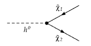
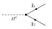
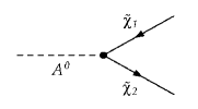
Figure 1: Tree-level diagrams for the decay of neutral Higgs bosons $h$, $H$ and $A$ to charginos $\tilde{\chi}^{+}_{1}$ and $\tilde{\chi}^{-}_{2}$.

The tree-level decay width for the two-body decay $h_{k}\rightarrow\tilde{\chi}^{+}_{i}\tilde{\chi}^{-}_{j}$ can therefore be written as

$$\mathit{\Gamma}^{\mathrm{tree}}(h_{k}\rightarrow\tilde{\chi}^{+}_{i}\tilde{\chi}^{-}_{j})=\, \frac{1}{16\pi m_{h_{k}}^{3}}\,\left((|C^{R}_{ijh_{k}}|^{2}+|C^{L}_{ijh_{k}}|^{2})\kappa(m_{h_{k}}^{2},m_{\tilde{\chi}^{\pm}_{i}}^{2},m_{\tilde{\chi}^{\pm}_{j}}^{2})\,\right.\big{(}m_{h_{k}}^{2}$$

$$-m_{\tilde{\chi}^{\pm}_{i}}^{2}-m_{\tilde{\chi}^{\pm}_{j}}^{2}\big{)}\left.-4C^{R}_{ijh_{k}}C^{L}_{ijh_{k}}(-1)^{\delta_{k3}}m_{\tilde{\chi}^{\pm}_{i}}m_{\tilde{\chi}^{\pm}_{j}}\right),$$ (92)

where

$$\kappa(x,y,z)=((x-y-z)^{2}-4yz)^{1/2}.$$ (93)

As explained in Sec. 2, we ensure the correct on-shell properties of the mixed neutral Higgs bosons by the use of finite wave function normalisation factors $\bf\hat{Z}_{ij}$, which contain universal propagator-type contributions up to the two-loop level. With the aim to investigate the effect of the genuine vertex contributions for this process, we will compare our full one-loop result to an improved Born result which incorporates the (process-independent) normalisation factors $\bf\hat{Z}_{ij}$. Accordingly, we define the improved Born result by summing over the tree-level amplitudes for the three neutral Higgs bosons $h_{k}$ weighted by the appropriate $\bf\hat{Z}$ factor,

$$\hat{G}_{\tilde{\chi}^{+}_{i}\tilde{\chi}^{-}_{j}h_{a}}^{\rm Imp.Born}=\sum_{k}\hat{\bf Z}_{ak}G^{\rm Born}_{\tilde{\chi}^{+}_{i}\tilde{\chi}^{-}_{j}h_{k}}(M^{2}_{h_{a}}).$$ (94)

As mentioned above, by definition the $\bf\hat{Z}$ factors do not include contributions due to mixing with the neutral Goldstone boson or the $Z$ boson, and therefore the relevant one-loop contributions of this type must be explicitly included in the calculation.

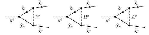
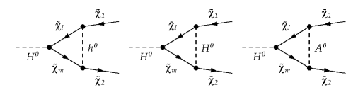
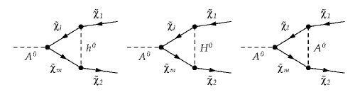
Figure 2: A selection of one-loop vertex diagrams for the decay of neutral Higgs bosons $h$, $H$ and $A$ to charginos $\tilde{\chi}^{+}_{1}$ and $\tilde{\chi}^{-}_{2}$.

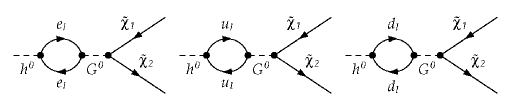
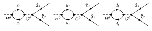
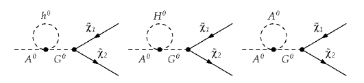
Figure 3: A selection of one-loop self-energy diagrams for the decay of neutral Higgs bosons $h$, $H$ and $A$ to charginos $\tilde{\chi}^{+}_{1}$ and $\tilde{\chi}^{-}_{2}$.

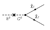
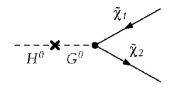
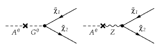
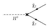
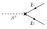
Figure 4: Counter-term diagrams for the decay of neutral Higgs bosons $h$, $H$ and $A$ to charginos $\tilde{\chi}^{+}_{1}$ and $\tilde{\chi}^{-}_{2}$.

The one-loop corrections therefore involve vertex diagrams, examples of which are shown in Fig. 2, and the self-energy diagrams involving the $Z$ and the Goldstone boson, examples of which are shown in Fig. 3. These are calculated following the procedure outlined earlier. In order to obtain UV finite results at the one-loop level, the three-point vertex function defined at tree-level in Eq. (89) must be renormalised, i.e. we need to calculate the diagrams shown in the bottom row of Fig. 4 for the vertex diagrams, and we also need to renormalise the self-energy corrections, i.e. we need to calculate the diagrams shown in the upper rows of Fig. 4.

The counterterm for the three-point vertex function defined in Eq. (89) is of the form

$$\delta G_{\tilde{\chi}^{+}_{i}\tilde{\chi}^{-}_{j}h_{k}}\equiv\omega_{R}\delta C^{R}_{ijh_{k}}+\omega_{L}(-1)^{\delta_{k3}}\delta C^{L}_{ijh_{k}},$$ (95)

and the coupling counterterms are given by

$$\delta C^{R/L}_{ijh_{k}}=\, \,C^{R/L}_{ijh_{k}}(\delta Z_{e}-\frac{\delta s_{W}}{s_{W}})+\frac{1}{2}\sum^{2}_{l=1}(\delta Z^{R/L}_{li}C^{R/L}_{ljh_{k}}+\delta\bar{Z}^{L/R}_{jl}C^{R/L}_{ilh_{k}})$$

$$+\frac{1}{2}(\delta Z_{h_{k}h}C^{R/L}_{ijh}+\delta Z_{h_{k}H}C^{R/L}_{ijH}+\delta Z_{h_{k}A}C^{R/L}_{ijA}+\delta Z_{h_{k}G}C^{R/L}_{ijG}),$$ (96)

where, in analogy to Eqs. (90) and (91),

$$C^{R}_{ijG}=\, \,C^{L^{\dagger}}_{ijG}=\frac{e}{\sqrt{2}s_{W}}c_{ijG},$$

$$c_{ijG}=\, i(-c_{\beta_{n}}U_{j2}V_{i1}+s_{\beta_{n}}U_{j1}V_{i2}).$$ (97)

Here $\delta Z_{e}$ and $\delta s_{W}$ are defined in Eqs. (43) and (41) respectively, and for the chargino field renormalisation constants, given in Eqs. (63) and (65), we have dropped the “$\pm$” as our tree-level diagrams do not contain any neutralinos. Note that the parameter renormalisation which enters these renormalisation constants is performed in the NCC scheme where the relevant counterterms are defined in Eqs. (85) to (87). The Higgs field renormalisation constants $\delta Z_{hh}$, $\delta Z_{hH}$, etc. appearing in Eq. (96) are linear combinations of the field renormalisation constants $\delta Z_{\mathcal{H}_{1}}^{\overline{\mathrm{DR}}}$, $\delta Z_{\mathcal{H}_{2}}^{\overline{\mathrm{DR}}}$ given in Eqs. (24) and (25), as specified in Ref. [69].

In order to account for the mixing of the neutral Higgs bosons, the result for the amplitude is obtained by summing over the contributions of the three neutral Higgs bosons, multiplied with the corresponding wave function normalisation factors $\bf\hat{Z}_{ij}$, and by furthermore adding the mixing contributions of the Higgs boson with the Goldstone boson and the Z boson,

$$\hat{G}_{\tilde{\chi}^{+}_{i}\tilde{\chi}^{-}_{j}h_{a}}^{\rm Imp.\,1-Loop}=\, \sum_{k}\hat{\bf Z}_{ak}\bigg{(}\hat{G}^{\rm 1PI}_{\tilde{\chi}^{+}_{i}\tilde{\chi}^{-}_{j}h_{k}}(M^{2}_{h_{a}})+\hat{G}^{\rm G,Z,se}_{h_{k}\tilde{\chi}^{+}_{i}\tilde{\chi}^{-}_{j}}(m^{2}_{h_{k}})\bigg{)}.$$ (98)

Here $\hat{G}^{\rm 1PI}_{\tilde{\chi}^{+}_{i}\tilde{\chi}^{-}_{j}h_{k}}$ contains both the tree-level and the complete one-loop contributions in the MSSM, and $M^{2}_{h_{a}},M^{2}_{h_{b}},M^{2}_{h_{c}}$ denote the loop-corrected masses, while $m^{2}_{h_{k}}$ refers to the tree-level masses, see Refs. [79, 80] for further details.

Since the virtual contributions to the decay width in Eq. (98) may involve virtual photons giving rise to IR divergences, we add the corresponding bremsstrahlung contribution from diagrams with real photon emission, as shown in Fig. 5. In this way we obtain the complete 1-loop result for the decay width,

$$\mathit{\Gamma}^{\rm Full}=\mathit{\Gamma}^{\rm\rm Imp.\,1-Loop}(h_{a}\to\tilde{\chi}^{+}_{i}\tilde{\chi}^{-}_{j})+\mathit{\Gamma}^{\rm Imp.\,Born}(h_{a}\to\tilde{\chi}^{+}_{i}\tilde{\chi}^{-}_{j}\gamma).$$ (99)

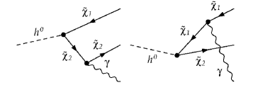
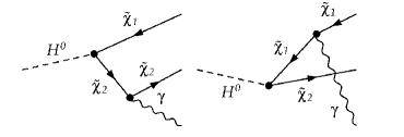
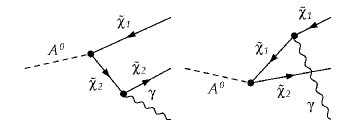
Figure 5: Diagrams for the decay of neutral Higgs bosons $h$, $H$ and $A$ to charginos $\tilde{\chi}^{+}_{1}$ and $\tilde{\chi}^{-}_{2}$ with real photon emission.

We have compared our result for the general case of complex parameters to the existing result that was restricted to the case of real parameters, given in Ref. [44], and obtainable via the package HFOLD [45]. There the renormalisation prescriptions used for the chargino and neutralino mixing matrices, for $\tan\beta$ (where the renormalisation condition given in Ref. [109] has been applied) and for the charge renormalisation differ from the ones used in the present work. The numerical evaluation in Ref. [44] was carried out in the SPS 1a benchmark scenario [110]. We find agreement between our result and the result of Ref. [44] within the expected accuracy.

For the numerical analysis of our results, we first consider the effects of the phases $\phi_{A_{t}}$, $M_{1}$ and $\mu$ for the parameters as defined in Tab. 2 (as mentioned above, we use the convention where the phase of the parameter $M_{2}$ is rotated away). In Fig. 6 we show our results for $\Gamma(h_{2}\to\tilde{\chi}_{1}^{+}\tilde{\chi}_{2}^{-})$ as a function of the phases $\phi_{A_{t}}$, $M_{1}$ and $\mu$. The full result corresponding to Eq. (99) is compared with the improved Born result based on the amplitude given in Eq. (94). As mentioned above, the improved Born result incorporates higher-order contributions not only from the calculation of the mass of the decaying Higgs boson, but we have also dressed the lowest-order result with the universal wave function normalisation factors $\bf\hat{Z}_{ij}$. As one can see in Fig. 6, the dominant contribution to the dependence of the decay width on the three phases $\phi_{A_{t}}$, $\phi_{M_{1}}$ and $\phi_{\mu}$ is already present in the improved Born result. Despite the fact that $\phi_{A_{t}}$ only enters at loop level, its numerical impact on the decay width is found to be very significant, which is a consequence of the large (Yukawa enhanced) stop loop corrections in the Higgs sector. Compared to the decay width at $\phi_{A_{t}}=0$, the full MSSM one-loop corrected decay width is modified by up to 11% and 40% upon varying $\phi_{A_{t}}$ for $M_{\tilde{q}_{3}}=600\,\,\mathrm{GeV}$ and 800 GeV, respectively. Note that here the larger impact of the phase at $M_{\tilde{q}_{3}}=800\,\,\mathrm{GeV}$ is due to a threshold effect, as the mass of the decaying Higgs lies very close to the mass of the stops. The deviations from the improved Born result amount up to 3% and 1% for $M_{\tilde{q}_{3}}=600\,\,\mathrm{GeV}$ and 800 GeV, respectively.

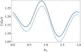
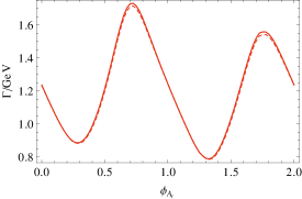
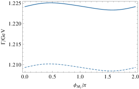
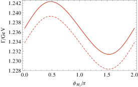
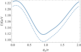
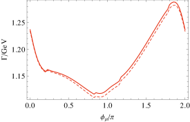
Figure 6: Decay width in GeV for $h_{2}\to\tilde{\chi}_{1}^{+}\tilde{\chi}_{2}^{-}$ as a function of the phases $\phi_{A_{t}}$ (upper), $\phi_{M_{1}}$ (middle) and $\phi_{\mu}$ (lower). The solid (dashed) lines show the 1-loop corrected (improved Born) results for $M_{\tilde{q}_{3}}=600$ (blue, left) and 800 (red, right) GeV.

The effects induced by the phase $M_{1}$, on the other hand, are relatively small. The shift compared to the decay width with $\phi_{M_{1}}=0$ and the deviations from the improved Born result are both at the percent level for $M_{\tilde{q}_{3}}=600\,\,\mathrm{GeV}$, and at the sub-percent level for $M_{\tilde{q}_{3}}=800\,\,\mathrm{GeV}$. As in the case of $\phi_{A_{t}}$, the phase of $M_{1}$ only arises in the expressions for the decay width at loop level, however the lower sensitivity of the decay width to this phase as compared to $\phi_{A_{t}}$ is expected as the pertinent loops are not Yukawa enhanced.

Variation of the phase of $\mu$ can in principle give rise to larger effects on the decay width of up to 8% and 10%, and deviations of 2% and 1% from the improved Born result, for $M_{\tilde{q}_{3}}=600\,\,\mathrm{GeV}$ and $M_{\tilde{q}_{3}}=800\,\,\mathrm{GeV}$, respectively, as it appears in the tree level couplings. However, taking into account the tight constraints on this phase from the EDM bounds discussed earlier, the impact of the phase variation on the decay width is reduced to the sub-percent level. The kinks seen in the bottom right-hand plot of Fig. 6 showing the dependence of the decay width on $\phi_{\mu}$ for $M_{\tilde{q}_{3}}=800\,\,\mathrm{GeV}$ arise due to the crossing of the masses of $h_{2}$ and $h_{3}$ at these points.

Accordingly, the phase having the most important impact on the decay width $\Gamma(h_{2}\to\tilde{\chi}_{1}^{+}\tilde{\chi}_{2}^{-})$ is $\phi_{A_{t}}$. Due to the prospective difficulty in resolving the decays of $h_{2}$ and $h_{3}$ experimentally, we have further investigated the dependence of the sum of the two decay widths, $\Gamma(h_{2}\to\tilde{\chi}_{1}^{+}\tilde{\chi}_{2}^{-})+\Gamma(h_{3}\to\tilde{\chi}_{1}^{+}\tilde{\chi}_{2}^{-})$, on $\phi_{A_{t}}$. As shown in Fig. 7, the marked dependence on $\phi_{A_{t}}$ is also present for the sum of the two decay widths, giving rise to shifts of up to 9% and 48% for $M_{\tilde{q}_{3}}=600\,\,\mathrm{GeV}$ and 800 GeV, respectively.

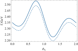
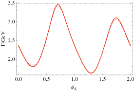
Figure 7: Sum of the decay widths in GeV for $h_{2}\to\tilde{\chi}_{1}^{+}\tilde{\chi}_{2}^{-}$ and $h_{3}\to\tilde{\chi}_{1}^{+}\tilde{\chi}_{2}^{-}$ as a function of the phase $\phi_{A_{t}}$. The solid (dashed) lines show the 1-loop corrected (improved Born) results for $M_{\tilde{q}_{3}}=600$ (blue, left) and 800 (red, right) GeV.

We now turn to the impact of the renormalisation procedure on our final result, i.e. we investigate the numerical relevance of the consistent treatment of the absorptive parts, which, as discussed in the previous section, affects in particular the field renormalisation prescription. In Fig. 8 we plot

$$\frac{\delta\mathit{\Gamma}}{\mathit{\Gamma}}=\frac{\mathit{\Gamma}^{\rm Full}-\mathit{\Gamma}^{\rm Imp.\,Born}}{\mathit{\Gamma}^{\rm Imp.\,Born}},$$ (100)

where we compare the result including the absorptive parts with an approximation where the absorptive parts are neglected. For unpolarised charginos in the final state, the proper treatment of the absorptive parts affects the decay width by, at most, 0.4%. In Fig. 8 we display the decay width for polarised charginos in the final state, $\Gamma(h_{2}\to\tilde{\chi}_{1,L}^{+}\tilde{\chi}_{2,R}^{-})$. We find that the numerical impact of the proper treatment of the absorptive parts can amount up to a 3% effect in the decay width. On the other hand, as expected, the effect is seen to vanish for the case of real parameters, i.e. $\phi_{A_{t}}=0,\pi$. The spikes seen in these plots arise due to the fact that at these values of $\phi_{A_{t}}$ the masses of the $h_{2}$ and $h_{3}$ bosons cross. The spikes are seen to vanish for example on changing $M_{\tilde{q}_{3}}$ to 520 GeV, as the Higgs masses no longer cross for any value of $\phi_{A_{t}}$, shown in the lower row of Fig. 8. While there may be a chance to determine the polarisation of charginos through the angular distribution of their decays products, a detailed study of the prospects at the LHC is yet to be undertaken.

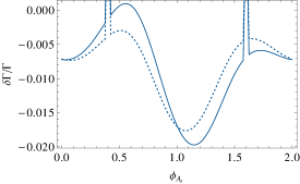
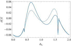
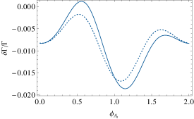
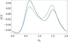
Figure 8: Ratio of the 1-loop corrected decay width to the tree-level decay width, as defined in Eq. (100), for $h_{2}\to\tilde{\chi}_{1,L}^{+}\tilde{\chi}_{2,R}^{-}$ as a function of the phase of $A_{t}$, $\phi_{A_{t}}$, showing the effect of absorptive parts of the self-energies in the chargino field renormalisation constants. The solid (dotted) line indicates the result with (without) taking the absorptive part into account. Parameters are as in Tab. 2, except $M_{\tilde{q}_{3}}=500\,\,\mathrm{GeV}$ for the upper plots and $M_{\tilde{q}_{3}}=520\,\,\mathrm{GeV}$ for the lower plots.

4.2 Chargino production at a future Linear Collider

As a second example, we now investigate chargino production at a Linear Collider, $\sigma(\mathit{e}^{+}\mathit{e}^{-}\to\tilde{\chi}_{i}^{+}\tilde{\chi}_{j}^{-})$. High-precision measurements of this process in the clean experimental environment of an $e^{+}e^{-}$ Linear Collider could be crucial for uncovering the fundamental parameters of this sector and for determining the nature of the underlying physics. A treatment addressing the most general case of complex parameters is mandatory in this context.

At leading order, in the limit of massless electrons, the process $\sigma(\mathit{e}^{+}\mathit{e}^{-}\to\tilde{\chi}_{1}^{+}\tilde{\chi}_{2}^{-})$ is described by the two diagrams shown in Fig. 9 (there is one additional diagram for the $\tilde{\chi}_{1}^{+}\tilde{\chi}_{1}^{-}$ and $\tilde{\chi}_{2}^{+}\tilde{\chi}_{2}^{-}$ final states). The transition matrix element can be written as [111],

$$\mathcal{M}_{\alpha\beta}(e^{+}e^{-}\to\tilde{\chi}^{+}_{i}\tilde{\chi}^{-}_{j})=i\frac{e^{2}}{s}Q_{\alpha\beta}\left[\bar{v}(e^{+})\gamma_{\mu}\omega_{\alpha}u(e^{-})\right]\left[\bar{u}(\tilde{\chi}^{-}_{j})\gamma^{\mu}\omega_{\beta}v(\tilde{\chi}^{+}_{i})\right],$$ (101)

in terms of the helicity amplitudes $Q_{\alpha\beta}$, where $\alpha$ refers to the chirality of the $e^{+}e^{-}$ current, $\beta$ to that of the $\tilde{\chi}_{i}^{+}\tilde{\chi}_{j}^{-}$ current, and summation over $\alpha$ and $\beta$ is implied.

$$Q_{LL}=\, \,\delta_{ij}+D_{Z}G_{L}C^{L}_{\tilde{\chi}^{+}_{i}\tilde{\chi}_{j}^{-}Z}$$

$$Q_{RL}=\, \,\delta_{ij}+D_{Z}G_{R}C^{L}_{\tilde{\chi}^{+}_{i}\tilde{\chi}_{j}^{-}Z}$$

$$Q_{LR}=\, \,\delta_{ij}+D_{Z}G_{L}\left(C^{R}_{\tilde{\chi}^{+}_{i}\tilde{\chi}_{j}^{-}Z}\right)^{*}+D_{\tilde{\nu}}\frac{1}{2s_{W}^{2}}\left(C^{R}_{\tilde{\nu}_{e}e^{+}\tilde{\chi}_{i}^{-}}\right)^{*}C^{R}_{\tilde{\nu}_{e}e^{+}\tilde{\chi}_{j}^{-}},$$

$$Q_{RR}=\, \,\delta_{ij}+D_{Z}G_{R}\left(C^{R}_{\tilde{\nu}_{e}e^{+}\tilde{\chi}_{i}^{-}}\right)^{*}.$$ (102)

The $Z\tilde{\chi}^{+}_{i}\tilde{\chi}^{-}_{j}$ and $e\tilde{\nu}_{e}\tilde{\chi}^{+}_{i}$ couplings are given by

$$C^{L}_{\tilde{\chi}^{+}_{i}\tilde{\chi}_{j}^{-}Z}=\, s_{W}^{2}\delta_{ij}-U^{*}_{j1}U_{i1}-\frac{1}{2}U^{*}_{j2}U_{i2},$$

$$C^{R}_{\tilde{\chi}^{+}_{i}\tilde{\chi}_{j}^{-}Z}=\, C^{L}_{\tilde{\chi}^{+}_{i}\tilde{\chi}_{j}^{-}Z}(U\to V^{*}),$$

$$C^{R}_{\tilde{\nu}_{e}e^{+}\tilde{\chi}_{i}^{-}}=\, -V_{i1},$$ (103)

and $G_{L}$, $G_{R}$, $D_{Z}$ and $D_{\tilde{\nu}}$ are defined via

$$G_{L}=\, \frac{s_{W}^{2}-\tfrac{1}{2}}{s_{W}^{2}c_{W}^{2}}, G_{R}=\, \frac{1}{c_{W}^{2}}\,,$$

$$D_{Z}=\, \frac{s}{s-M_{Z}^{2}}, D_{\tilde{\nu}}=\, \frac{s}{t-m_{\tilde{\nu}}^{2}}.$$ (104)

Here $D_{Z}$ and $D_{\tilde{\nu}}$ refer to the propagators of the $Z$ boson and sneutrino, respectively, in terms of the Mandelstam variables $s$ and $t$, and we can neglect the non-zero $Z$ width for the considered energies. The tree-level cross section in the unpolarised case is then obtained by summing over the squared matrix elements,

$$\sigma^{\rm tree}=\frac{\kappa^{1/2}(s,m_{\tilde{\chi}^{+}_{i}},m_{\tilde{\chi}^{-}_{j}})}{64\pi^{2}s^{2}}\int d\Omega\sum_{\alpha,\beta}|{\mathcal{M}_{\alpha\beta}}|^{2}.$$ (105)

Figure 9: Tree-level diagrams for the production of charginos $\tilde{\chi}^{+}_{1}$ and $\tilde{\chi}^{-}_{2}$ at the LC.

The one-loop corrections involve self-energy, vertex and box diagrams, examples of which are shown in Fig. 10. The diagrams are calculated following the procedure outlined earlier.

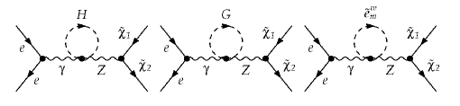
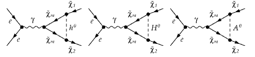
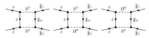
Figure 10: Example one-loop self-energy (upper), vertex (middle) and box (lower) diagrams for the production of charginos $\tilde{\chi}^{+}_{1}$ and $\tilde{\chi}^{-}_{2}$ at the LC.

In order to obtain finite results at one-loop, we need to renormalise the couplings defined at tree-level in Eq. (101), i.e. we need to calculate the diagrams shown in Fig.11.

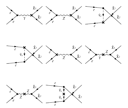
Figure 11: Counterterm diagrams for the production of charginos $\tilde{\chi}^{+}_{1}$ and $\tilde{\chi}^{-}_{2}$ at the LC.

This involves renormalising the $\gamma\tilde{\chi}^{+}_{i}\tilde{\chi}^{-}_{j}$, $Z\tilde{\chi}^{+}_{i}\tilde{\chi}^{-}_{j}$ and $e\tilde{\nu}_{e}\tilde{\chi}^{+}_{i}$ vertices as follows,

$$\delta\mathrm{G}^{L}_{\tilde{\chi}^{+}_{i}\tilde{\chi}_{j}^{-}\gamma}=\, \frac{ie}{2}\left(\delta_{ij}\left(2\delta Z_{e}+\delta Z_{\gamma\gamma}\right)-\frac{\delta Z_{Z\gamma}}{c_{W}s_{W}}C^{L}_{\tilde{\chi}^{+}_{i}\tilde{\chi}_{j}^{-}Z}+\delta Z^{L}_{ij}+\delta\bar{Z}^{L}_{ij}\right),$$

$$\delta\mathrm{G}^{L}_{\tilde{\chi}^{+}_{i}\tilde{\chi}_{j}^{-}Z}=\, \frac{-ie}{c_{W}s_{W}}\bigg{(}\delta C^{L}_{\tilde{\chi}^{+}_{i}\tilde{\chi}_{j}^{-}Z}+C^{L}_{\tilde{\chi}^{+}_{i}\tilde{\chi}_{j}^{-}Z}\left(\delta Z_{e}-\frac{\delta c_{W}}{c_{W}}-\frac{\delta s_{W}}{s_{W}}+\frac{\delta Z_{ZZ}}{2}\right)$$

$$-\delta_{ij}\frac{c_{W}s_{W}}{2}\delta Z_{\gamma Z}+\frac{1}{2}\sum_{n=1,2}\left(\delta Z^{L}_{nj}C^{L}_{\tilde{\chi}^{+}_{i}\tilde{\chi}_{n}^{-}Z}+C^{L}_{\tilde{\chi}^{+}_{n}\tilde{\chi}_{j}^{-}Z}\delta\bar{Z}^{L}_{in}\right)\bigg{)}.$$ (106)

where the analogous right-handed parts are obtained by the replacement $L\to R$. Furthermore,

$$\delta\mathrm{G}^{R}_{\tilde{\nu}_{e}e^{+}\tilde{\chi}_{i}^{-}}=\, \frac{ie\delta_{ij}}{s_{W}}\bigg{(}C^{R}_{\tilde{\nu}_{e}e^{+}\tilde{\chi}_{i}^{-}}\bigg{(}\delta Z_{e}-\frac{\delta s_{W}}{s_{W}}+\frac{1}{2}\left(\delta Z_{\tilde{\nu}_{e}}+\delta Z^{e^{*}}_{L}\right)$$

$$+\frac{1}{2}\left(\delta Z^{R}_{1i}V^{*}_{12}+\delta Z^{R}_{2i}V^{*}_{22}\right)\bigg{)}+\delta C^{R}_{\tilde{\nu}_{e}e^{+}\tilde{\chi}_{i}^{-}}\bigg{)},$$

$$\delta\mathrm{G}_{\overline{\tilde{\nu}}_{i}\tilde{\nu}_{j}}=\, i\delta_{ij}\left(\frac{1}{2}(\delta Z_{\tilde{\nu}_{i}}+\delta Z^{*}_{\tilde{\nu}_{i}})p^{2}-\delta m_{\tilde{\nu}_{i}}^{2}-\frac{m_{\tilde{\nu}_{i}}^{2}}{2}(\delta Z_{\tilde{\nu}_{i}}+\delta Z^{*}_{\tilde{\nu}_{i}})\right),$$ (107)

for $\tilde{\nu}_{i}=\tilde{\nu}_{e},\tilde{\nu}_{\mu},\tilde{\nu}_{\tau}$, and the counterterm contributions of the coupling factors are given by

$$\delta C^{L}_{\tilde{\chi}^{+}_{i}\tilde{\chi}_{j}^{-}Z}=\, \delta C^{R}_{\tilde{\chi}^{+}_{i}\tilde{\chi}_{j}^{-}Z}=2s_{W}\delta s_{W}\delta_{ij},$$

$$\delta C^{R}_{\tilde{\nu}_{e}e^{+}\tilde{\chi}_{i}^{-}}=\, 0.$$ (108)

Note that again for brevity we drop the $\pm$ for the chargino field renormalisation constants. Using this prescription to renormalise the vertices we obtain UV-finite results.

As the incoming and outgoing particles are charged, in order to obtain an infra-red finite result one must furthermore include soft photon radiation, which introduces the dependence on a cut-off. Using the phase-space slicing method the full phase space for the real photonic corrections can be divided into a soft, a hard collinear and a hard non-collinear (IR finite) region,

$$\sigma^{\rm brems}=\sigma^{\rm soft}(\Delta E)+\sigma^{\rm hard}_{\rm coll}(\Delta E,\Delta\theta)+\sigma^{\rm hard}_{\rm non-coll}(\Delta E,\Delta\theta).$$ (109)

Here the singular soft and hard collinear regions are defined by $E<\Delta E$ and $\theta<\Delta\theta$, respectively. Accordingly, the full cross section at next-to-leading order, including also the virtual contributions, is given by

$$\sigma^{\rm full}=\sigma^{\rm tree}+\sigma^{\rm virt+soft}(\Delta E)+\sigma^{\rm hard}_{\rm coll}(\Delta E,\Delta\theta)+\sigma^{\rm hard}_{\rm non-coll}(\Delta E,\Delta\theta).$$ (110)

Since in our analysis we are particularly interested in the relative size of the weak SUSY corrections, it is useful to consider a “reduced genuine SUSY cross-section”, as defined by the SPA convention [90], where the numerically large logarithmic terms of the QED-type corrections depending on $\Delta E$ and the terms proportional to $L_{e}\equiv\log s/m_{e}^{2}$ are subtracted in a consistent and gauge-independent way. Accordingly, our numerical analysis below is done for the quantity (see Refs. [90, 47])

$$\sigma^{\rm weak}=\, \,\sigma^{\rm tree}+\sigma^{\rm virt+soft}(\Delta E)+\sigma^{\Delta E},$$ (111)

$$\sigma^{\Delta E}=\, -\frac{\alpha}{\pi}\sigma^{\rm tree}\bigg{(}\frac{3}{2}L_{e}+\log\frac{4(\Delta E)^{2}}{s}(L_{e}-1+\Delta_{\gamma})\bigg{)},$$ (112)

where $\Delta_{\gamma}$ is given by the coefficient of the terms in the soft photon correction involving $\Delta E$ that arise from final state radiation (ISR) and from the interference between initial and final state radiation (IFI). To be more explicit, we express the soft photon contribution as a sum of initial state radiation (ISR), FSR and IFI,

$$\sigma^{\rm soft}\,=\,-\sigma^{\rm tree}\frac{\alpha}{4\pi^{2}}\left(\delta_{\rm soft}^{\rm ISR}+\delta_{\rm soft}^{\rm FSR}+\delta_{\rm soft}^{\rm IFI}\right).$$ (113)

Defining $\delta_{\rm ISR}$ etc., in terms of the soft photon integrals $I_{ij}$ [81],

$$\delta_{\rm soft}^{\rm ISR}\,=\, \,I_{p_{1}p_{1}}+I_{p_{2}p_{2}}-2I_{p_{1}p_{2}}\,,$$

$$\delta_{\rm soft}^{\rm FSR}=\, I_{k_{1}k_{1}}+I_{k_{2}k_{2}}-2I_{k_{1}k_{2}}\,,$$

$$\delta_{\rm soft}^{\rm IFI}\,=\, \,-2\left(I_{p_{1}k_{1}}+I_{p_{2}k_{2}}-I_{p_{1}k_{2}}-I_{p_{2}k_{1}}\right)\,,$$ (114)

the quantity $\Delta_{\gamma}$ can be obtained by taking the coefficient of $4\pi\log\frac{4(\Delta E)^{2}}{s}$ in $\delta_{\rm soft}^{\rm FSR}+\delta_{\rm soft}^{\rm IFI}$.

In the soft limit, the photonic contributions can be factorised into analytically integrable expressions proportional to the tree-level cross-section for $\sigma(\mathit{e}^{+}\mathit{e}^{-}\to\tilde{\chi}_{i}^{+}\tilde{\chi}_{j}^{-})$. In our calculation carried out with FormCalc the contributions from soft photon radiation have been incorporated using the soft photon factor as given explicitly in Ref. [81].

Restricting our general result for complex MSSM parameters to the special case of vanishing phases, we have compared with the results given in Refs. [47, 48], which were evaluated in the $\rm SPS1a^{\prime}$ benchmark scenario. The renormalisation prescription in Ref. [47] differs from the one used in the present work in the renormalisation of the chargino and neutralino mixing matrices as well as of the electric charge and $\tan\beta$. Furthermore, a different choice has been made in Ref. [47] for the masses chosen as input in the selectron / sneutrino sector (as a consequence, the sneutrino mass in Ref. [47] receives a shift at the one-loop level, while we have chosen an on-shell condition for the sneutrino mass). On the other hand, in the special case of real parameters our renormalisation prescription is the same as the one used in Ref. [48], with the exception of the renormalisation of $\tan\beta$. We find numerical agreement within the expected accuracy with the results given in Refs. [47, 48].

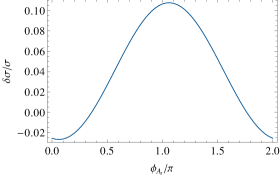
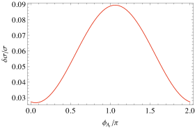
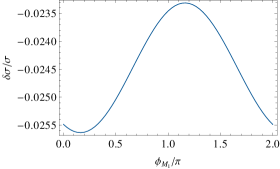
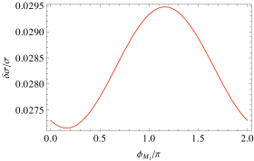
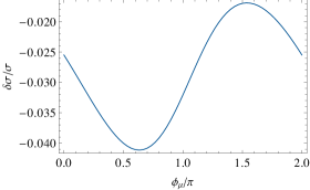
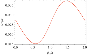
Figure 12: $\delta\sigma/\sigma$ for $e^{+}e^{-}\to\tilde{\chi}_{1}^{+}\tilde{\chi}_{2}^{-}$ as a function of the phases $\phi_{A_{t}}$ (upper), $\phi_{M_{1}}$ (middle) and $\phi_{\mu}$ (lower row) for $M_{\tilde{q}_{3}}=600$ (left) and 800 (right) GeV.

We now turn to the investigation of our results for the case of complex MSSM parameters. In particular, we study the relative size of the one-loop corrections,

$$\frac{\delta\sigma}{\sigma}=\frac{(\sigma^{\rm weak}-\sigma^{\rm tree})}{\sigma^{\rm tree}}$$ (115)

as a function of $\phi_{A_{t}}$, $\phi_{\mu}$ and $\phi_{M_{1}}$, for a $\sqrt{s}=800\,\,\mathrm{GeV}$ LC. In Fig. 12, the dependence on each of the phases is seen to be qualitatively the same for $M_{\tilde{q}_{3}}=600\,\,\mathrm{GeV}$ and 800 GeV. In the case of $\phi_{A_{t}}$, the dependence is sizeable, due to the Yukawa enhancement for the stop loops, leading to effects of up to $\sim 12\%$ for $M_{\tilde{q}_{3}}=600\,\,\mathrm{GeV}$ and up to $\sim 6\%$ for $M_{\tilde{q}_{3}}=800\,\,\mathrm{GeV}$. For the EDM-allowed regions of $\phi_{M_{1}}$, which enters only at loop-level, and $\mu$, which is highly constrained, the numerical impact of the phase variations is rather small, at most $\sim 0.2\%$ for $\phi_{M_{1}}$. Thus, particularly for low values of $M_{\tilde{q}_{3}}$, the phenomenologically most relevant effect arises from varying the phase $\phi_{A_{t}}$.

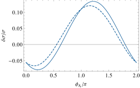
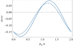
Figure 13: $\delta\sigma/\sigma$ for $e^{+}e^{-}\to\tilde{\chi}_{1}^{+}\tilde{\chi}_{2}^{-}$ (left) and $e^{+}e^{-}\to\tilde{\chi}_{1,L}^{+}\tilde{\chi}_{2,R}^{-}$ (right) as a function of the phase $\phi_{A_{t}}$, for $M_{\tilde{q}_{3}}=500\,\,\mathrm{GeV}$, including (solid) and ignoring (dashed) the absorptive part of the loop integrals in the field renormalisation.

In Fig. 13 we plot $\delta\sigma/\sigma$ as a function of $\phi_{A_{t}}$, comparing the results of including and ignoring the absorptive parts of the loop integrals in the field renormalisation. The left plot shows the unpolarised cross section for $e^{+}e^{-}\to\tilde{\chi}_{1}^{+}\tilde{\chi}_{2}^{-}$, while the right plot shows the result for specific polarisation states of the produced charginos, $e^{+}e^{-}\to\tilde{\chi}_{1,L}^{+}\tilde{\chi}_{2,R}^{-}$. The impact of properly accounting for the absorptive parts of the loop integrals in the field renormalisation is clearly visible in Fig. 13. The resulting difference amounts to up to $\sim 2\%$, which could be phenomenologically relevant at linear collider precisions. Thus, a consistent inclusion of the absorptive parts of loop integrals is not only desirable from a conceptual point of view, but can also give rise to phenomenologically relevant effects in the MSSM with complex parameters. Another feature that can be seen in Fig. 13 is the fact that for $\phi_{A_{t}}=\pi$ (in the present case where all other phases are set to zero) the results of including and ignoring the absorptive parts coincide. This is as expected, confirming that in the case of real parameters the absorptive parts can be neglected, see Sec. 4.1.

We find that the numerical impact of properly incorporating the absorptive parts increases with an increasing hierarchy between the parameters $M_{1}$, $M_{2}$ and $\mu$. This is illustrated in Fig. 14, where the cross section for $e^{+}e^{-}\to\tilde{\chi}_{1}^{+}\tilde{\chi}_{2}^{-}$ is shown as a function of $\mu$. The difference between the results including and neglecting the absorptive parts is seen to increase for increasing $\mu$. The behaviour of the results around $\mu=480\,\,\mathrm{GeV}$ is caused by a threshold effect due to the sneutrino mass lying in this region.

5 Conclusions

We have derived a renormalisation scheme for the chargino and neutralino sector of the MSSM that is suitable for the most general case of complex parameters. We have put particular emphasis on a consistent treatment of imaginary parts, which arise on the one hand from the complex parameters of the model and on the other hand from absorptive parts of loop integrals. We have demonstrated that products of imaginary parts can contribute to predictions for physical observables in the MSSM already at the one-loop level and therefore need to be taken into account in order to obtain complete one-loop results.

Concerning the parameter renormalisation in the chargino and neutralino sector, we have shown that the phases of the parameters in the chargino and neutralino sector do not need to be renormalised at the one-loop level. We have therefore adopted a renormalisation scheme where only the absolute values of the parameters $M_{1}$, $M_{2}$ and $\mu$ are subject to the renormalisation procedure. In order to perform an on-shell renormalisation for those parameters one needs to choose three out of the six masses in the chargino and neutralino sector that are renormalised on-shell, while the predictions for the physical masses of the other three particles receive loop corrections. We have demonstrated, using the examples of gaugino-like and higgsino like scenarios with complex parameters, that the appropriate choice for the mass parameters used as input for the on-shell conditions depends both on the process and the region of MSSM parameter space under consideration. In order to avoid unphysically large contributions to the counterterms and the mass predictions one needs to choose for the on-shell renormalisation one bino-like, one wino-like and one higgsino-like particle. We have provided full expressions for the renormalisation constants of $|M_{1}|$, $|M_{2}|$ and $|\mu|$ for the case where $M_{1}$ and $\mu$ can be complex (i.e., we have adopted the convention where the phase of $M_{2}$ has been rotated away) and for all possible combinations of charginos and neutralinos being chosen on-shell.

For the field renormalisation, the consistent incorporation of absorptive parts gives rise to the fact that full on-shell conditions, which ensure that all mixing contributions of the involved fields vanish on-shell, can only be satisfied if independent field renormalisation constants are chosen for incoming and outgoing fields. If instead one works with a scheme where those renormalisation constants are related to each other by the usual hermiticity relations, non-trivial corrections associated with the external legs of the considered diagrams (i.e., finite wave function normalisation factors) need to be incorporated in order to obtain the correct on-shell properties of the incoming and outgoing particles.

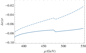
Figure 14: $\delta\sigma/\sigma$ for $e^{+}e^{-}\to\tilde{\chi}_{1}^{+}\tilde{\chi}_{2}^{-}$ as a function of $\mu$, for $M_{\tilde{q}_{3}}=500\,\,\mathrm{GeV}$ and $\phi_{A_{t}}=\pi/4$, including (solid) and ignoring (dashed) the absorptive part of the loop integrals in the field renormalisation.

Within the described renormalisation framework we have derived complete one-loop results for the processes $h_{a}\to\tilde{\chi}_{i}^{+}\tilde{\chi}_{j}^{-}$ (supplemented by Higgs-propagator corrections up to the two-loop level) and $e^{+}e^{-}\to\tilde{\chi}_{i}^{+}\tilde{\chi}_{j}^{-}$ in the MSSM with complex parameters. For both processes we have investigated the dependence of the results on the phases of the complex parameters. In particular, we have analysed in this context the numerical relevance of the absorptive parts of loop integrals.

Concerning our results for heavy Higgs decays to charginos, $h_{a}\to\tilde{\chi}_{i}^{+}\tilde{\chi}_{j}^{-}$, which may be of interest for SUSY Higgs searches at the LHC, we find that the phase variations have a significant numerical impact on the prediction for the decay width. In particular, varying the phase $\phi_{A_{t}}$, which is so far almost unconstrained by the EDMs, can lead to effects of up to 40% in the decay width. We find that the impact of the absorptive parts in the field renormalisation constants is most pronounced for the case of polarised charginos in the final state, for which the impact of a proper treatment of the absorptive parts can amount up to a 3% effect in the decay width.

For chargino pair-production at an $e^{+}e^{-}$ Linear Collider, $e^{+}e^{-}\to\tilde{\chi}_{i}^{+}\tilde{\chi}_{j}^{-}$, we find that the dependence of the cross-section on the phase $\phi_{A_{t}}$ is sizable, yielding effects of up to 12% in our example. The impact of a proper treatment of the absorptive parts in the field renormalisation constants turns out to be numerically relevant in view of the prospective experimental accuracy of measurements at a future Linear Collider. We find effects of 2–5% in our numerical example. Our results for the one-loop contributions to chargino pair-production at a Linear Collider for the general case of complex MSSM parameters may also be of interest for investigating the accuracy with which the parameters of the MSSM Lagrangian can be determined from high-precision measurements at a Linear Collider, since in this context the incorporation of higher-order effects in the theoretical predictions, which lead to a non-trivial dependence on a variety of MSSM parameters, is inevitable.

References

- [1] G. Aad et al. [ATLAS Collaboration], Phys. Lett. B [arXiv:1207.7214 [hep-ex]].
- [2] S. Chatrchyan et al. [CMS Collaboration], Phys. Lett. B [arXiv:1207.7235 [hep-ex]].
- [3] The Tevatron New-Phenomena and Higgs Working Group [CDF and D0 Collaborations], arXiv:1207.0449 [hep-ex].
- [4] H. Baer, V. Barger and A. Mustafayev, Phys. Rev. D 85 (2012) 075010 [arXiv:1112.3017 [hep-ph]], A. Arbey, M. Battaglia, A. Djouadi, F. Mahmoudi and J. Quevillon, Phys. Lett. B 708 (2012) 162 [arXiv:1112.3028 [hep-ph]], M. Carena, S. Gori, N. R. Shah and C. E. M. Wagner, JHEP 1203 (2012) 014 [arXiv:1112.3336 [hep-ph]], P. Draper, P. Meade, M. Reece and D. Shih, Phys. Rev. D 85 (2012) 095007 [arXiv:1112.3068 [hep-ph]], O. Buchmueller, R. Cavanaugh, A. De Roeck, M. J. Dolan, J. R. Ellis, H. Flacher, S. Heinemeyer and G. Isidori et al., Eur. Phys. J. C 72 (2012) 2020 [arXiv:1112.3564 [hep-ph]], M. Kadastik, K. Kannike, A. Racioppi and M. Raidal, JHEP 1205 (2012) 061 [arXiv:1112.3647 [hep-ph]], C. Strege, G. Bertone, D. G. Cerdeno, M. Fornasa, R. Ruiz de Austri and R. Trotta, JCAP 1203 (2012) 030 [arXiv:1112.4192 [hep-ph]], J. Cao, Z. Heng, D. Li and J. M. Yang, Phys. Lett. B 710 (2012) 665 [arXiv:1112.4391 [hep-ph]], F. Brummer and W. Buchmuller, JHEP 1205 (2012) 006 [arXiv:1201.4338 [hep-ph]], D. Carmi, A. Falkowski, E. Kuflik and T. Volansky, JHEP 1207 (2012) 136 [arXiv:1202.3144 [hep-ph]], J. Ellis and K. A. Olive, Eur. Phys. J. C 72 (2012) 2005 [arXiv:1202.3262 [hep-ph]], N. Desai, B. Mukhopadhyaya and S. Niyogi, arXiv:1202.5190 [hep-ph], J. -J. Cao, Z. -X. Heng, J. M. Yang, Y. -M. Zhang and J. -Y. Zhu, JHEP 1203 (2012) 086 [arXiv:1202.5821 [hep-ph]], T. Cheng, J. Li, T. Li, D. V. Nanopoulos and C. Tong, arXiv:1202.6088 [hep-ph], M. Asano, S. Matsumoto, M. Senami and H. Sugiyama, Phys. Rev. D 86 (2012) 015020 [arXiv:1202.6318 [hep-ph]], P. P. Giardino, K. Kannike, M. Raidal and A. Strumia, JHEP 1206 (2012) 117 [arXiv:1203.4254 [hep-ph]], M. A. Ajaib, I. Gogoladze, F. Nasir and Q. Shafi, Phys. Lett. B 713 (2012) 462 [arXiv:1204.2856 [hep-ph]], M. Carena, S. Gori, N. R. Shah, C. E. M. Wagner and L. -T. Wang, JHEP 1207 (2012) 175 [arXiv:1205.5842 [hep-ph]], A. Fowlie, M. Kazana, K. Kowalska, S. Munir, L. Roszkowski, E. M. Sessolo, S. Trojanowski and Y. -L. S. Tsai, Phys. Rev. D 86 (2012) 075010 [arXiv:1206.0264 [hep-ph]], K. Hagiwara, J. S. Lee and J. Nakamura, JHEP 1210 (2012) 002 [arXiv:1207.0802 [hep-ph]], A. Arbey, M. Battaglia, A. Djouadi and F. Mahmoudi, JHEP 1209 (2012) 107 [arXiv:1207.1348 [hep-ph]], M. R. Buckley and D. Hooper, Phys. Rev. D 86 (2012) 075008 [arXiv:1207.1445 [hep-ph]], S. Akula, P. Nath and G. Peim, Phys. Lett. B 717 (2012) 188 [arXiv:1207.1839 [hep-ph]], J. Cao, Z. Heng, J. M. Yang and J. Zhu, JHEP 1210 (2012) 079 [arXiv:1207.3698 [hep-ph]], O. Buchmueller, R. Cavanaugh, M. Citron, A. De Roeck, M. J. Dolan, J. R. Ellis, H. Flacher and S. Heinemeyer et al., arXiv:1207.7315 [hep-ph], Z. Heng, arXiv:1210.3751 [hep-ph], U. Haisch and F. Mahmoudi, arXiv:1210.7806 [hep-ph].
- [5] S. Heinemeyer, O. Stål and G. Weiglein, Phys. Lett. B 710 (2012) 201 [arXiv:1112.3026 [hep-ph]].
- [6] R. Benbrik, M. G. Bock, S. Heinemeyer, O. Stål, G. Weiglein and L. Zeune, arXiv:1207.1096 [hep-ph].
- [7] P. Bechtle, S. Heinemeyer, O. Stål, T. Stefaniak, G. Weiglein and L. Zeune, arXiv:1211.1955 [hep-ph].
-
[8]
A. Bottino, N. Fornengo and S. Scopel,
Phys. Rev. D 85 (2012) 095013
[arXiv:1112.5666 [hep-ph]],
M. Drees, arXiv:1210.6507 [hep-ph]. - [9] G. Aad et al. [ATLAS Collaboration], arXiv:1208.0949 [hep-ex], JHEP 1207 (2012) 167 [arXiv:1206.1760 [hep-ex]].
- [10] S. Chatrchyan et al. [CMS Collaboration], JHEP 1210 (2012) 018 [arXiv:1207.1798 [hep-ex]], Phys. Rev. Lett. 109 (2012) 171803 [arXiv:1207.1898 [hep-ex]].
- [11] G. Aad et al. [ATLAS Collaboration], arXiv:1208.1447 [hep-ex], arXiv:1208.2590 [hep-ex], arXiv:1208.2884 [hep-ex], arXiv:1208.3144 [hep-ex].
- [12] S. Chatrchyan et al. [CMS Collaboration], Phys. Rev. D 86 (2012) 072010 [arXiv:1208.4859 [hep-ex]], arXiv:1209.6620 [hep-ex].
- [13] J. Beringer et al. [Particle Data Group Collaboration], Phys. Rev. D 86 (2012) 010001.
- [14] H. K. Dreiner, S. Heinemeyer, O. Kittel, U. Langenfeld, A. M. Weber and G. Weiglein, Eur. Phys. J. C 62 (2009) 547 [arXiv:0901.3485 [hep-ph]].
- [15] T. Ibrahim and P. Nath, Rev. Mod. Phys. 80 (2008) 577 [arXiv:0705.2008 [hep-ph]].
- [16] O. Kittel, J. Phys. Conf. Ser. 171 (2009) 012094 [arXiv:0904.3241 [hep-ph]].
- [17] G. Moortgat-Pick, K. Rolbiecki and J. Tattersall, Phys. Rev. D 83 (2011) 115012 [arXiv:1008.2206 [hep-ph]].
- [18] H. Dreiner, O. Kittel, S. Kulkarni and A. Marold, Phys. Rev. D 83 (2011) 095012 [arXiv:1011.2449 [hep-ph]].
- [19] S. Bornhauser, M. Drees, H. Dreiner, O. J. P. Eboli, J. S. Kim and O. Kittel, Eur. Phys. J. C 72 (2012) 1887 [arXiv:1110.6131 [hep-ph]].
- [20] A. C. Fowler and G. Weiglein, JHEP 1001 (2010) 108 [arXiv:0909.5165 [hep-ph]].
- [21] T. Fritzsche, S. Heinemeyer, H. Rzehak and C. Schappacher, Phys. Rev. D 86 (2012) 035014 [arXiv:1111.7289 [hep-ph]].
- [22] S. Heinemeyer, F. von der Pahlen and C. Schappacher, Eur. Phys. J. C 72 (2012) 1892 [arXiv:1112.0760 [hep-ph]].
- [23] S. Heinemeyer and C. Schappacher, Eur. Phys. J. C 72 (2012) 2136 [arXiv:1204.4001 [hep-ph]].
- [24] A. Bharucha, S. Heinemeyer, F. von der Pahlen and C. Schappacher, Phys. Rev. D 86 (2012) 075023 [arXiv:1208.4106 [hep-ph]].
- [25] A. Bharucha, arXiv:1202.6284 [hep-ph].
- [26] A. Bharucha, J. Kalinowski, G. Moortgat-Pick, K. Rolbiecki and G. Weiglein, arXiv:1208.1521 [hep-ph].
- [27] A. B. Lahanas, K. Tamvakis and N. D. Tracas, Phys. Lett. B 324 (1994) 387 [arXiv:hep-ph/9312251].
- [28] D. Pierce and A. Papadopoulos, Phys. Rev. D 50 (1994) 565 [arXiv:hep-ph/9312248].
- [29] D. Pierce and A. Papadopoulos, Nucl. Phys. B 430 (1994) 278 [arXiv:hep-ph/9403240].
- [30] H. Eberl, M. Kincel, W. Majerotto and Y. Yamada, Phys. Rev. D 64 (2001) 115013 [arXiv:hep-ph/0104109].
- [31] T. Fritzsche and W. Hollik, Eur. Phys. J. C 24 (2002) 619 [arXiv:hep-ph/0203159].
- [32] W. Oller, H. Eberl, W. Majerotto and C. Weber, Eur. Phys. J. C 29 (2003) 563 [arXiv:hep-ph/0304006].
- [33] M. Drees, W. Hollik and Q. Xu, JHEP 0702 (2007) 032 [arXiv:hep-ph/0610267].
- [34] A. C. Fowler, PhD Thesis, 2010, http://etheses.dur.ac.uk/449/1/Thesis_AFowler.pdf.
- [35] A. Chatterjee, M. Drees, S. Kulkarni and Q. Xu, Phys. Rev. D 85 (2012) 075013 [arXiv:1107.5218 [hep-ph]].
- [36] F. Moortgat, S. Abdullin and D. Denegri, arXiv:hep-ph/0112046.
- [37] M. Bisset, J. Li, N. Kersting, R. Lu, F. Moortgat and S. Moretti, JHEP 0908 (2009) 037 [arXiv:0709.1029 [hep-ph]].
- [38] H. Baer, M. Bisset, D. Dicus, C. Kao and X. Tata, Phys. Rev. D 47, 1062 (1993).
- [39] H. Baer, M. Bisset, C. Kao and X. Tata, Phys. Rev. D 50, 316 (1994) [arXiv:hep-ph/9402265].
- [40] M. Bisset, M. Guchait and S. Moretti, Eur. Phys. J. C 19, 143 (2001) [arXiv:hep-ph/0010253].
- [41] G. L. Bayatian et al. [CMS Collaboration], J. Phys. G 34 (2007) 995.
- [42] S. Gennai, S. Heinemeyer, A. Kalinowski, R. Kinnunen, S. Lehti, A. Nikitenko and G. Weiglein, Eur. Phys. J. C 52 (2007) 383 [arXiv:0704.0619 [hep-ph]].
- [43] R. Y. Zhang, W. G. Ma, L. H. Wan and Y. Jiang, Phys. Rev. D 65 (2002) 075018 [arXiv:hep-ph/0201132].
- [44] H. Eberl, W. Majerotto and Y. Yamada, Phys. Lett. B 597 (2004) 275 [arXiv:hep-ph/0405187].
- [45] W. Frisch, H. Eberl, H. Hlucha, Comput. Phys. Commun. 182 (2011) 2219-2226. [arXiv:1012.5025 [hep-ph]].
- [46] K. Desch, J. Kalinowski, G. A. Moortgat-Pick, M. M. Nojiri and G. Polesello, [arXiv:hep-ph/0312069].
- [47] W. Oller, H. Eberl and W. Majerotto, Phys. Rev. D 71 (2005) 115002 [arXiv:hep-ph/0504109].
- [48] T. Fritzsche, PhD Thesis, Cuvillier Verlag, Göttingen 2005, ISBN 3-86537-577-4.
- [49] P. Osland and A. Vereshagin, Phys. Rev. D 76 (2007) 036001 [arXiv:0704.2165 [hep-ph]].
- [50] K. Rolbiecki and J. Kalinowski, Phys. Rev. D 76 (2007) 115006 [arXiv:0709.2994 [hep-ph]].
- [51] S. Dimopoulos and D. W. Sutter, Nucl. Phys. B 452 (1995) 496 [arXiv:hep-ph/9504415]
- [52] V. D. Barger, T. Falk, T. Han, J. Jiang, T. Li and T. Plehn, Phys. Rev. D 64 (2001) 056007 [arXiv:hep-ph/0101106].
- [53] C. A. Baker et al., Phys. Rev. Lett. 97 (2006) 131801 [arXiv:hep-ex/0602020].
- [54] B. C. Regan, E. D. Commins, C. J. Schmidt and D. DeMille, Phys. Rev. Lett. 88 (2002) 071805.
- [55] W. C. Griffith, M. D. Swallows, T. H. Loftus, M. V. Romalis, B. R. Heckel and E. N. Fortson, Phys. Rev. Lett. 102 (2009) 101601.
- [56] W. Hollik, J. I. Illana, S. Rigolin and D. Stockinger, Phys. Lett. B 416, 345 (1998) [arXiv:hep-ph/9707437]; Phys. Lett. B 425 (1998) 322 [arXiv:hep-ph/9711322].
- [57] D. A. Demir, O. Lebedev, K. A. Olive, M. Pospelov and A. Ritz, Nucl. Phys. B 680 (2004) 339 [arXiv:hep-ph/0311314].
- [58] D. Chang, W. Y. Keung and A. Pilaftsis, Phys. Rev. Lett. 82 (1999) 900 [Erratum-ibid. 83, 3972 (1999)] [arXiv:hep-ph/9811202]; A. Pilaftsis, Phys. Lett. B 471 (1999) 174 [arXiv:hep-ph/9909485].
- [59] O. Lebedev, K. A. Olive, M. Pospelov and A. Ritz, Phys. Rev. D 70 (2004) 016003 [arXiv:hep-ph/0402023].
- [60] Y. Li, S. Profumo and M. Ramsey-Musolf, JHEP 1008 (2010) 062 [arXiv:1006.1440 [hep-ph]].
- [61] J. Ellis, F. Moortgat, G. Moortgat-Pick, J. M. Smillie and J. Tattersall, Eur. Phys. J. C 60 (2009) 633 [arXiv:0809.1607 [hep-ph]].
- [62] T. Ibrahim and P. Nath, Phys. Lett. B 418 (1998) 98 [arXiv:hep-ph/9707409]; T. Ibrahim and P. Nath, Phys. Rev. D 57 (1998) 478 [arXiv:hep-ph/9708456].
- [63] M. Brhlik, G. J. Good and G. L. Kane, Phys. Rev. D 59 (1999) 115004 [arXiv:hep-ph/9810457].
- [64] Y. Li, S. Profumo and M. Ramsey-Musolf, Phys. Lett. B 673 (2009) 95 [arXiv:0811.1987 [hep-ph]].
- [65] G. Moortgat-Pick, K. Rolbiecki, J. Tattersall and P. Wienemann, JHEP 1001 (2010) 004 [arXiv:0908.2631 [hep-ph]].
- [66] F. F. Deppisch and O. Kittel, JHEP 1006 (2010) 067 [arXiv:1003.5186 [hep-ph]].
- [67] A. Bartl, H. Fraas, O. Kittel and W. Majerotto, Eur. Phys. J. C 36 (2004) 233 [arXiv:hep-ph/0402016].
- [68] O. Kittel, G. Moortgat-Pick, K. Rolbiecki, P. Schade and M. Terwort, Eur. Phys. J. C 72 (2012) 1854 [arXiv:1108.3220 [hep-ph]].
- [69] M. Frank, T. Hahn, S. Heinemeyer, W. Hollik, H. Rzehak and G. Weiglein, JHEP 0702 (2007) 047 [arXiv:hep-ph/0611326].
- [70] A. Brignole, Phys. Lett. B 281 (1992) 284.
- [71] M. Frank, S. Heinemeyer, W. Hollik and G. Weiglein, arXiv:hep-ph/0212037.
- [72] A. Freitas and D. Stockinger, arXiv:hep-ph/0210372.
- [73] S. Heinemeyer, W. Hollik, G. Weiglein, Eur. Phys. J. C9 (1999) 343-366. [hep-ph/9812472].
- [74] S. Heinemeyer, W. Hollik, G. Weiglein, Comput. Phys. Commun. 124 (2000) 76-89. [hep-ph/9812320].
- [75] G. Degrassi, S. Heinemeyer, W. Hollik, P. Slavich, G. Weiglein, Eur. Phys. J. C28 (2003) 133-143. [arXiv:hep-ph/0212020 [hep-ph]].
- [76] T. Hahn, S. Heinemeyer, W. Hollik, H. Rzehak, G. Weiglein, Comput. Phys. Commun. 180 (2009) 1426-1427.
- [77] R. Barate et al. [LEP Working Group for Higgs boson searches and ALEPH and DELPHI and L3 and OPAL Collaborations], Phys. Lett. B 565 (2003) 61 [hep-ex/0306033].
- [78] S. Schael et al. [ALEPH and DELPHI and L3 and OPAL and LEP Working Group for Higgs Boson Searches Collaborations], Eur. Phys. J. C 47 (2006) 547 [hep-ex/0602042].
- [79] K. E. Williams and G. Weiglein, Phys. Lett. B 660 (2008) 217 [arXiv:0710.5320 [hep-ph]].
- [80] K. E. Williams, H. Rzehak and G. Weiglein, Eur. Phys. J. C 71 (2011) 1669 [arXiv:1103.1335 [hep-ph]].
- [81] A. Denner, Fortsch. Phys. 41 (1993) 307-420. [arXiv:0709.1075 [hep-ph]].
- [82] J. Guasch, W. Hollik, J. Sola, JHEP 0210 (2002) 040. [hep-ph/0207364].
- [83] B. A. Kniehl, A. Pilaftsis, Nucl. Phys. B474 (1996) 286-308. [hep-ph/9601390].
- [84] A. Denner, T. Sack, Nucl. Phys. B347 (1990) 203-216.
- [85] P. Gambino, P. A. Grassi, F. Madricardo, Phys. Lett. B454 (1999) 98-104. [hep-ph/9811470].
- [86] Y. Yamada, Phys. Rev. D64 (2001) 036008. [hep-ph/0103046].
- [87] B. A. Kniehl and A. Sirlin, Phys. Lett. B 673 (2009) 208 [arXiv:0901.0114 [hep-ph]].
- [88] D. Espriu, J. Manzano and P. Talavera, Phys. Rev. D 66 (2002) 076002 [arXiv:hep-ph/0204085].
- [89] Y. Zhou, Mod. Phys. Lett. A 21 (2006) 2763 [arXiv:hep-ph/0502186].
- [90] J. A. Aguilar-Saavedra et al., Eur. Phys. J. C 46 (2006) 43 [arXiv:hep-ph/0511344].
- [91] J. Kublbeck, M. Bohm, and A. Denner, Comput. Phys. Commun. 60 (1990) 165–180.
- [92] A. Denner, H. Eck, O. Hahn, and J. Kublbeck, Nucl.Phys. B387 (1992) 467–484.
- [93] J. Kublbeck, H. Eck, and R. Mertig, Nucl.Phys.Proc.Suppl. 29A (1992) 204–208.
- [94] T. Hahn, Comput. Phys. Commun. 140 (2001) 418–431, [arXiv:hep-ph/0012260].
- [95] T. Hahn and C. Schappacher, Comput. Phys. Commun. 143 (2002) 54–68, [arXiv:hep-ph/0105349].
- [96] T. Hahn and M. Perez-Victoria, Comput. Phys. Commun. 118 (1999) 153–165, [arXiv:hep-ph/9807565].
- [97] T. Hahn, Comput. Phys. Commun. 178 (2008) 217–221, [arXiv:hep-ph/0611273].
- [98] T. Hahn and M. Rauch, Nucl. Phys. Proc. Suppl. 157 (2006) 236–240, [arXiv:hep-ph/0601248].
- [99] W. Siegel, Phys. Lett. B84 (1979) 193.
- [100] W. Siegel, Phys. Lett. B94 (1980) 37.
- [101] D. Stöckinger, JHEP 03 (2005) 076, [arXiv:hep-ph/0503129].
- [102] F. del Aguila, A. Culatti, R. Munoz Tapia, and M. Perez-Victoria, Nucl. Phys. B537 (1999) 561–585, [arXiv:hep-ph/9806451]
- [103] K. Nakamura et al. [ Particle Data Group Collaboration ], J. Phys. G G37 (2010) 075021.
- [104] M. Lancaster [Tevatron Electroweak Working Group and for the CDF and D0 Collaborations], arXiv:1107.5255 [hep-ex].
- [105] J. S. Lee, A. Pilaftsis, M. S. Carena, S. Y. Choi, M. Drees, J. R. Ellis and C. E. M. Wagner, Comput. Phys. Commun. 156 (2004) 283 [arXiv:hep-ph/0307377].
- [106] S. Berge, W. Bernreuther, B. Niepelt, H. Spiesberger, [arXiv:1108.0670 [hep-ph]].
- [107] S. Berge, W. Bernreuther, Phys. Lett. B671 (2009) 470-476. [arXiv:0812.1910 [hep-ph]].
- [108] S. Berge, W. Bernreuther, J. Ziethe, Phys. Rev. Lett. 100 (2008) 171605. [arXiv:0801.2297 [hep-ph]].
- [109] A. Dabelstein, Z. Phys. C67 (1995) 495-512. [arXiv:hep-ph/9409375 [hep-ph]].
- [110] B. C. Allanach, M. Battaglia, G. A. Blair, M. S. Carena, A. De Roeck, A. Dedes, A. Djouadi, D. Gerdes et al., Eur. Phys. J. C25 (2002) 113-123. [hep-ph/0202233].
- [111] S. Y. Choi, A. Djouadi, M. Guchait, J. Kalinowski, H. S. Song, P. M. Zerwas, Eur. Phys. J. C14 (2000) 535-546. [hep-ph/0002033].