Mass-degenerate Higgs bosons at 125 GeV in the Two-Higgs-Doublet Model

Abstract

The analysis of the Higgs boson data by the ATLAS and CMS Collaborations appears to exhibit an excess of $h\to\gamma\gamma$ events above the Standard Model (SM) expectations; whereas no significant excess is observed in $h\to ZZ^{*}\to\textrm{four lepton}$ events, albeit with large statistical uncertainty due to the small data sample. These results (assuming they persist with further data) could be explained by a pair of nearly mass-degenerate scalars, one of which is a SM-like Higgs boson and the other is a scalar with suppressed couplings to $W^{+}W^{-}$ and $ZZ$. In the two Higgs doublet model, the observed $\gamma\gamma$ and $ZZ^{*}\to\textrm{four lepton}$ data can be reproduced by an approximately degenerate CP-even ($h$) and CP-odd ($A$) Higgs boson for values of $\sin(\beta-\alpha)$ near unity and $0.7\mathrel{\;{\hbox{\raise 1.50696pt\hbox{$<$}}\kern-3.8889pt\kern-3.8889pt\hbox{\lower 2.79857pt\hbox{$\sim$}}}\;}\tan\beta\mathrel{\;{\hbox{\raise 1.50696pt\hbox{$<$}}\kern-3.8889pt\kern-3.8889pt\hbox{\lower 2.79857pt\hbox{$\sim$}}}\;}1$. An enhanced $\gamma\gamma$ signal can also arise in cases where $m_{h}\simeq m_{H}$, $m_{H}\simeq m_{A}$, or $m_{h}\simeq m_{H}\simeq m_{A}$. Since the $ZZ^{*}\to\textrm{four lepton}$ signal derives primarily from a SM-like Higgs boson whereas the $\gamma\gamma$ signal receives contributions from two (or more) nearly mass-degenerate states, one would expect a slightly different invariant mass peak in the $ZZ^{*}\to\textrm{four lepton}$ and $\gamma\gamma$ channels. The phenomenological consequences of such models can be tested with additional Higgs data that will be collected at the LHC in the near future.

1 Introduction

The ATLAS ATLASHiggs and CMS CMSHiggs collaborations have recently announced the discovery of a new boson with the properties approximating those of the Standard Model Higgs boson ($h$) hhg . The cleanest channels for the observation of the Higgs boson are via the rare decays $h\to\gamma\gamma$ and $h\to ZZ^{*}\to\ell^{+}\ell^{-}\ell^{\prime\,+}\ell^{\prime\,-}$ (where $\ell=e$ or $\mu$). Evidence for Higgs boson production and decay is also seen in $h\to WW^{*}\to\ell^{+}\nu\ell^{-}\overline{\nu}$. Using this data, both ATLAS and CMS have compared the observed values of $\sigma\times{\rm BR}$ for the Higgs boson production and decay into the various final states, relative to the corresponding Standard Model predictions. Including both the 2011 and 2012 data sets, both collaboration observe excesses of the $\gamma\gamma$ channels ATLASgg ; CMSgg , whereas the $WW^{*}$ and $ZZ^{*}$ channels are consistent with Standard Model expectations.

Although the excess in the $\gamma\gamma$ channel is not yet statistically significant, it is instructive to consider mechanisms that could enhance the $\gamma\gamma$ channel while not affecting the Standard Model–like results for $pp$ into vector boson pairs. Note that the Higgs boson couples to $\gamma\gamma$ through a one-loop process, whereas it couples to vector bosons at tree level. Thus, one could enhance the $\gamma\gamma$ signal by proposing new charged particles beyond the Standard Model that couple to the Higgs boson manyrefs1 . Such particles would contribute in the loop amplitude for $h\to\gamma\gamma$ and could potentially enhance the $h\to\gamma\gamma$ branching ratio. However, in such a scenario one must check that the same particles do not contribute significantly to the $gg\to h$ production mechanism (which is also generated by a one-loop process). Otherwise, one might find that $\sigma\times{\rm BR}$ for Higgs production and decay into $WW^{*}$ and $ZZ^{*}$ is enhanced or suppressed with respect to the Standard Model, which is disfavored by the observed data.

Alternatively, one could enhance the $\gamma\gamma$ signal by increasing the branching ratio for Higgs decay into $\gamma\gamma$ with respect to that of the Standard Model. One way to accomplish this is to reduce the corresponding Higgs branching ratios into other decay channels. The most effective mechanism of this type is one where the dominant Higgs decay rate into $b\bar{b}$ pairs is significantly reduced. Specific examples can be found in Ref. manyrefs2 .

In this paper, we investigate a third mechanism that can potentially enhance the $\gamma\gamma$ signal while not affecting the $WW^{*}$ and $ZZ^{*}$ signal. For simplicity, we assume that the Higgs sector is CP-conserving. Suppose that there exist two nearly mass-degenerate scalars, a CP-even state $h$ and a CP-odd state $A$. If the properties of $h$ are approximately given by those of the Standard Model Higgs boson, then the observed $\sigma\times BR(h\to VV^{*})$ [where $V=W$ or $Z$] should be consistent with Standard Model Higgs production and decay, due to the fact that there are no tree-level $AVV$ couplings. On the other hand, the production cross section for $gg\to A$ is typically larger than the production cross section for $gg\to h$, and the decay $A\to\gamma\gamma$ is mediated at one-loop by the top quark loop. Thus, if $m_{h}\simeq m_{A}$, then both the $h$ and the $A$ will appear in the $\gamma\gamma$ signal, thereby yielding an enhanced $\gamma\gamma$ signal.

The same mechanism of enhancing the $\gamma\gamma$ signal applies more generally to any Higgs sector that only contains Higgs doublets (and possibly Higgs singlets) with no higher Higgs multiplets. If there exists a CP-even state $h$ whose properties are approximately given by those of the Standard Model Higgs boson, then this one state will approximately saturate the sum rule for $hVV$ couplings sumrule , in which case the couplings of any other neutral Higgs boson (whether CP-even, CP-odd or an arbitrary mixture thereof) to $VV$ will be highly suppressed. In such a case, $h$ and a second scalar state are approximately mass-degenerate, then both can contribute to an enhanced $\gamma\gamma$ signal observed at the LHC, whereas only $h$ production and decay yields a significant $ZZ^{*}\to\rm{four~{}leptons}$ signal.

In this paper, we consider the implications of the CP-conserving two Higgs doublet extension of the Standard Model (2HDM). There is already a substantial literature that analyzes the implications of the present Higgs data in the framework of the 2HDM sher ; 2HDMrefs . We shall address the question of whether the presence of nearly mass-degenerate neutral scalars of the 2HDM can be responsible for an enhanced $\gamma\gamma$ signal. Such a mechanism was first proposed in Ref. Gunion:2012gc in the context of the non-minimal supersymmetric extension of the Standard Model (NMSSM), and was also recently applied in the context of the 2HDM in an independent study degenerate2 .

What is the origin of the approximate mass degeneracy of the two near-degenerate Higgs states? In most cases, the near-degeneracy is accidental. However, one could imagine that a near-mass-degenerate CP-even/CP-odd scalar pair might originate from a single complex scalar $\Phi^{0}$. The presence of a global U(1) symmetry would then yield identical masses for the real and imaginary parts of $\Phi^{0}$. If the explicit breaking of the global U(1) symmetry is small (perhaps due to loop corrections), the resulting CP-even and CP-odd scalars would end up as approximate mass-degenerate states. Whether the near-degeneracy is accidental or the result of an approximate symmetry, it is important to analyze the LHC Higgs data to determine if such a scenario is realized in nature or can be excluded. In Ref. Gunion:2012he , a set of diagnostic tools was developed that can be used to determine whether mass-degenerate Higgs states are present in the LHC Higgs data.

We begin our analysis by computing the $\sigma\times{\rm BR}$ for the production and decay of $h$ and $A$ separately, under the assumption that $m_{h}\simeq m_{A}\simeq 125$ GeV and the couplings of $h$ to $W^{+}W^{-}$ and $ZZ$ approximate the corresponding Standard Model Higgs boson couplings. We then determine the region of 2HDM parameter space in which the sum of the $h$ and $A$ signals into $\gamma\gamma$ match the enhanced rates suggested by the central values measured by the ATLAS and CMS Collaborations. We also check to see whether an excess in the $\gamma\gamma$ channel can be achieved with other mass degenerate scalars ($h$, $H$), ($H$, $A$) and ($h$, $H$, $A$). Under the assumption that mass-degenerate neutral Higgs states can be invoked to explain the excess in the $\gamma\gamma$ channel, we predict which additional Higgs channels must also exhibit deviations from their corresponding Standard Model predictions.

2 Setting up the 2HDM parameter scan

The 2HDM consists of two hypercharge-one scalar doublet fields, denoted by $\Phi_{a}$, where $a=1,2$ review . The Lagrangian of the most general 2HDM contains a scalar potential, with two real and one complex scalar squared-mass term and four real and three complex dimensionless self-couplings, and the most general set of dimension-4 Higgs-fermion Yukawa interactions. For example, the most general Yukawa Lagrangian, in terms of the quark mass-eigenstate fields, is:

$$-\mathscr{L}_{\rm Y}=\overline{U}_{L}\widetilde{\Phi}_{a}^{0}{\eta^{U}_{a}}U_{R}+\overline{D}_{L}K^{\dagger}\widetilde{\Phi}_{a}^{-}{\eta^{U}_{a}}U_{R}+\overline{U}_{L}K\Phi_{a}^{+}{\eta^{D\,\dagger}_{a}}D_{R}+\overline{D}_{L}\Phi_{a}^{0}{\eta^{D\,\dagger}_{a}}D_{R}+{\rm h.c.}\,,$$ (2.1)

where $\widetilde{\Phi}_{a}\equiv(\widetilde{\Phi}^{0}\,,\,\widetilde{\Phi}^{-})=i\sigma_{2}\Phi_{a}^{*}$ and $K$ is the CKM mixing matrix. In eq. (2.1), there is an implicit sum over the index $a=1,2$, and the $\eta^{U,D}$ are $3\times 3$ Yukawa coupling matrices. However, such models generically possess tree-level Higgs-mediated flavor-changing neutral currents (FCNCs), in conflict with experimental data that requires FCNC interactions to be significantly suppressed.

To avoid dangerous FCNC interactions in a natural way, we impose a $\mathbb{Z}_{2}$ symmetry on the dimension-4 terms of the Higgs Lagrangian in such a way that removes two of the four Yukawa coupling matrices of eq. (2.1). The corresponding symmetry consists of choosing one of the two Higgs fields to be odd under the $\mathbb{Z}_{2}$ symmetry. The resulting Higgs potential is given by:

$$V = m^{2}_{11}\Phi_{1}^{\dagger}\Phi_{1}+m^{2}_{22}\Phi_{2}^{\dagger}\Phi_{2}-\left(m^{2}_{12}\Phi_{1}^{\dagger}\Phi_{2}+{\rm h.c.}\right)+\tfrac{1}{2}\lambda_{1}\left(\Phi_{1}^{\dagger}\Phi_{1}\right)^{2}+\tfrac{1}{2}\lambda_{2}\left(\Phi_{2}^{\dagger}\Phi_{2}\right)^{2}$$ (2.2)

$$\qquad\qquad\qquad\qquad\qquad\qquad+\lambda_{3}\Phi_{1}^{\dagger}\Phi_{1}\Phi_{2}^{\dagger}\Phi_{2}+\lambda_{4}\Phi_{1}^{\dagger}\Phi_{2}\Phi_{2}^{\dagger}\Phi_{1}+\left[\tfrac{1}{2}\lambda_{5}\left(\Phi_{1}^{\dagger}\Phi_{2}\right)^{2}+{\rm h.c.}\right]\,,$$

where we have allowed for a softly-broken $\mathbb{Z}_{2}$ symmetry due to the presence of the term proportional to $m_{12}^{2}$. For simplicity, we shall assume that the potentially complex terms in eq. (2.2), $m_{12}^{2}$ and $\lambda_{5}$ are real, in which case the Higgs potential is CP-conserving. In addition, some of the fermion fields may also be odd under the $\mathbb{Z}_{2}$ symmetry, depending on which two of the four Yukawa coupling matrices are required to vanish. Different choices lead to different Yukawa interactions. In this paper, we focus on two different model choices, known in the literature as Type-I type1 ; hallwise and Type-II type2 ; hallwise . In the Type-I 2HDM, $\eta_{1}^{U}=\eta_{1}^{D}=0$ in eq. (2.1), which means that all quarks and leptons couple exclusively to $\Phi_{2}$. In the Type-II 2HDM, $\eta_{1}^{U}=\eta_{2}^{D}=0$ in eq. (2.1), which means that the up-type quarks couple exclusively to $\Phi_{2}$ and the down-type quarks and charged leptons couple exclusively to $\Phi_{1}$.

We assume that the parameters of the Higgs potential are chosen such that the SU(2)$\times$U(1) electroweak symmetry is broken to U(1) electromagnetism. The neutral Higgs fields then acquire vacuum expectation values, $\langle\Phi_{a}^{0}\rangle=v_{a}/\sqrt{2}$, where $v_{1}^{2}+v_{2}^{2}=4m_{W}^{2}/g^{2}=(246~{}{\rm GeV})^{2}$ and $\tan\beta\equiv v_{2}/v_{1}$. By convention, we choose $0\leq\beta\leq\tfrac{1}{2}\pi$. Expanding the Higgs potential about its minimum, we then diagonalize the resulting scalar squared-mass matrices. Three Goldstone boson states are eaten by the $W^{\pm}$ and $Z$ gauge bosons, leaving five physical degrees of freedom: a charged Higgs pair, $H^{\pm}$, two CP-even neutral Higgs states, $h$ and $H$ (defined such that $m_{h}\leq m_{H}$), and one CP-odd neutral Higgs boson $A$. In diagonalizing the CP-even neutral Higgs squared-mass matrix, one also obtains a CP-even Higgs mixing angle, $\alpha$. By convention, we take $|\alpha|\leq\pi/2$. In the Type-I and Type-II 2HDM, the Higgs-fermion couplings are flavor diagonal and depend on the two angles $\alpha$ and $\beta$ as shown in Table 1.

		Type-I							Type-II
		$h$		$A$		$H$			$h$		$A$		$H$
Up-type quarks		$\cos{\alpha}/\sin{{\beta}}$		$\phantom{-}\cot{\beta}$		$\sin{\alpha}/\sin{{\beta}}$			$\phantom{-}\cos{\alpha}/\sin{{\beta}}$		$\cot{\beta}$		$\sin{\alpha}/\sin{{\beta}}$
Down-type quarks and charged leptons		$\cos{\alpha}/\sin{{\beta}}$		$-\cot{\beta}$		$\sin{\alpha}/\sin{{\beta}}$			$-\sin{\alpha}/\cos{{\beta}}$		$\tan{\beta}$		$\cos{\alpha}/\cos{{\beta}}$

Table 1: Couplings of the fermions to the lighter and heavier CP-even scalars ($h$ and $H$), and the CP-odd scalar ($A$).

The aim of this paper is to scan the Type-I and Type-II 2HDM parameter spaces allowing the $\gamma\gamma$ signal resulting from the production of two near-mass-degenerate Higgs states to be enhanced above the Standard Model (SM) rate, while assuming that the corresponding $ZZ^{*}\to 4$ leptons (and $WW^{*}$) signal is approximately given by the corresponding SM rate. In general, given a final state $f$, we define $R_{f}$ as the ratio of the number of events predicted in the 2HDM with near-mass-degenerate Higgs states to that obtained in the SM:

$$R_{f}=\frac{N(pp\to f)_{\rm 2HDM}}{N(pp\to f)_{\rm SM}}.$$ (2.3)

Denoting the two near-mass-degenerate Higgs states by $h_{1}$ and $h_{2}$, we obtain

$$R_{f}=R^{h_{1}}_{f}+R^{h_{2}}_{f},$$ (2.4)

where

$$R^{S}_{f}=\frac{\sigma(pp\to S)_{\textrm{2HDM}}\ \textrm{BR}(S\to f)_{\textrm{2HDM}}}{\sigma(pp\to h_{\textrm{SM}})\ \textrm{BR}(h_{\textrm{SM}}\to f)},$$ (2.5)

for $S=h_{1}$, $h_{2}$ and $\sigma$ is the Higgs production cross section, BR the branching ratio, and $h_{\textrm{SM}}$ is the SM Higgs boson. In our analysis, we include all Higgs production mechanisms, namely, gluon-gluon fusion using HIGLU at NLO Spira:1995mt , vector boson fusion (VBF) LHCHiggs , Higgs production in association with either $W$, $Z$ or $t\bar{t}$ LHCHiggs , and $b\bar{b}$ fusion Harlander:2003ai .

Since we do not expect Higgs coupling measurements at the LHC to be better than about $20\%$ after the full 2012 data set is analyzed, we have performed our 2HDM scans under the assumption that

$$0.8<R_{ZZ}<1.2\,.$$ (2.6)

In the case where $h_{1}=h$ and $h_{2}=A$, the constraint imposed by our $R_{ZZ}$ assumption implies that the $ZZ^{*}\to 4$ leptons signal is due almost entirely to the production and decay of $h$, due to the absence of a tree-level $AZZ$ coupling. That is, the properties of the $h$ are SM-like. Remarkably, the same conclusions emerge in the case where both $h_{1}$ and $h_{2}$ are CP-even states. In this case, we find that one of the two CP-even states is SM-like, where the other has suppressed tree-level couplings to $ZZ$.

We perform our 2HDM scans separately for the Type-I and Type-II Higgs-fermion couplings, by scanning over the neutral and charged Higgs masses, the angles $\alpha$ and $\beta$ and the soft-breaking parameter $m_{12}^{2}$, subject to the constraint of eq. (2.6) and the near mass-degeneracy of two (or three) neutral Higgs bosons. If the two nearly mass-degenerate Higgs states are CP-even, then we shall assume that the mass difference of these states is large enough (compared to the corresponding Higgs boson widths) so that we can neglect possible interference effects in the production and decay process. This is not a significant constraint on our analysis, as the Higgs widths are significantly smaller than the experimental mass resolution of the ATLAS and CMS experiments.

In addition, the allowed points of our scans must also satisfy the known indirect experimental constraints on the Type-I and Type-II 2HDM. These constraints are described in Section 3. After imposing these requirements, we identify the surviving parameter regimes where the $\gamma\gamma$ signal is enhanced, and discuss additional Higgs phenomena that must be observed in order to confirm the scenarios advocated in this paper.

3 Constraints on the 2HDM parameters

In this section, we summarize the indirect experimental constraints on the CP-conserving 2HDM with Type-I and Type-II Higgs-fermion Yukawa couplings, respectively. First, we scan over the parameter space subject to the following three constraints: the Higgs scalar potential is (i) bounded from below vac1 ; (ii) satisfies tree-level unitarity unitarity ; and (iii) is consistent with constraints from the Peskin-Takeuchi $S$ and $T$ parameters Peskin:1991sw ; STHiggs as derived from electroweak precision observables lepewwg ; gfitter1 ; gfitter2 . Additional indirect 2HDM constraints arise from charged Higgs exchange contributions to processes involving the $b$ quark and $\tau$-lepton. Such processes yield constraints in the $m_{H^{\pm}}$–$\tan\beta$ plane. Consequently, if the rates for these processes are consistent with SM expectations, then the corresponding 2HDM constraints are (typically) relaxed in the limit of large $m_{H^{\pm}}$ due to the decoupling properties of the 2HDM decoupling . At present, there is an anomaly observed by the BaBar collaboration in the rate for $\overline{B}\to D^{(*)}\tau^{-}\overline{\nu}_{\tau}$ which deviates by 3.4 $\sigma$ (when $D$ and $D^{*}$ final states are combined) from the SM prediction Lees:2012xj . The observed deviation cannot be explained by a charged Higgs boson in the Type-II 2HDM. Indeed the analysis of Ref. Lees:2012xj excludes the Type-II 2HDM for any value of $\tan\beta/m_{H^{\pm}}$ at the $99.8\%$ CL. Until this observation is independently confirmed by the BELLE collaboration, we will not include this result among our 2HDM constraints.

A number of other observables in $B$ physics provide constraints in the $m_{H^{\pm}}$–$\tan\beta$ parameter plane. The most precise SM prediction for $R_{b}\equiv\Gamma(Z\to b\bar{b})/\Gamma(Z\to{\rm hadrons})$, including electroweak two-loop and QCD three-loop corrections, deviates by two standard deviations from the experimentally measured value Freitas:2012sy . The inclusion of 2HDM contributions could alleviate this discrepancy in particular regions of the parameter space Denner:1991ie ; Boulware:1991vp ; Grant:1994ak ; Haber:1999zh . Another constraining observable is the decay rate for $b\to s\gamma$. The theoretical prediction for $b\to s\gamma$ in the SM has been performed to order $\mathcal{O}(\alpha_{s}^{2})$ Misiak:2006zs and is in good agreement with the experimental result Asner:2010qj . However, due to theoretical uncertainties coming mainly from higher order QCD corrections and the uncertainties in the CKM matrix element, there is still some room for 2HDM contributions. Other $B$ observables such as $B$–$\bar{B}$ mixing data and the rate for $B^{+}\to\tau^{+}\nu_{\tau}$ also provide constraints on the 2HDM parameter space.

In the Type-II 2HDM, $R_{b}$ provides the most restrictive bound in the $m_{H^{\pm}}$–$\tan\beta$ plane in the small $\tan\beta$ region, as shown in Refs. Haber:1999zh ; gfitter1 . However, the strongest bound on the charged Higgs mass derives from the $b\to s\gamma$ measurement, which yields $m_{H^{\pm}}\gtrsim 360$ GeV at the $95\%$ CL almost independently of the value of $\tan\beta$ Mahm . In contrast, $B$–$\bar{B}$ mixing yields less constraining bounds in the $m_{H^{\pm}}$–$\tan\beta$ plane, whereas $B^{+}\to\tau^{+}\nu_{\tau}$ constrains mainly large values of $\tan\beta$ for small charged Higgs masses BB . In the Type-I 2HDM, the most restrictive bound in the $m_{H^{\pm}}$–$\tan\beta$ plane is due to $b\to s\gamma$ BB . In contrast to the Type-II model, there is no strong bound (independent of the value of $\tan\beta$) on the charged Higgs mass. Finally we note that all other experimental bounds on the Type-I 2HDM from $B$-physics observables were shown to be less restrictive BB ; gfitter1 .

With the exception of $B\to\tau^{+}\nu_{\tau}$ and $\overline{B}\to D^{(*)}\tau^{-}\overline{\nu}_{\tau}$ (where charged Higgs exchange contributes at tree-level), the 2HDM contributions to $B$ physics observables arise via one-loop radiative corrections. For such observables, it is always possible that constraints on the 2HDM parameter space could be relaxed due to cancellations in the loop from other sources of new physics. One of the well-known examples of this phenomenon is the partial cancellation of the charged Higgs loop and the chargino loop contributions to $b\to s\gamma$ in the MSSM bsgmssm . Thus, to be flexible in our presentation, we shall present results of our 2HDM scans with and without the bounds from $B$-physics and $R_{b}$. In the former case, the $95\%$ CL bounds from $B$-physics and $R_{b}$ are employed. We will denote our parameter scan as “constrained,” when all experimental and theoretical bounds are considered, and “unconstrained” when all except the $R_{b}$ and $B$-physics bounds are taken into account.

4 Degenerate $h$ and $A$

We begin by fixing $m_{A}=m_{h}=125\,\textrm{GeV}$. We scan over 2HDM parameters subject to eq. (2.6). As a consequence, the $h$ couplings to $W^{+}W^{-}$, $ZZ$ and $t\bar{t}$ cannot differ much from their SM values. The $\gamma\gamma$ signal is enhanced if the contribution from the $A$ is large; this can be achieved for values of $\tan{\beta}\mathrel{\;{\hbox{\raise 1.50696pt\hbox{$<$}}\kern-3.8889pt\kern-3.8889pt\hbox{\lower 2.79857pt\hbox{$\sim$}}}\;}1$. Thus, we focus our analysis on the region $0.5<\tan\beta<2$. Since $A$ does not couple to $ZZ$, the square of the $hZZ$ coupling, i.e. $\sin^{2}{(\beta-\alpha)}$, is constrained to be near its SM value. In the $\tan\beta$ parameter regime of interest, we find that $0.7\mathrel{\;{\hbox{\raise 1.50696pt\hbox{$<$}}\kern-3.8889pt\kern-3.8889pt\hbox{\lower 2.79857pt\hbox{$\sim$}}}\;}\sin^{2}{(\beta-\alpha)}<1$ for both Type-I and Type-II Higgs-fermion Yukawa couplings.

By convention (and without loss of generality), we define $\alpha$ and $\beta$ such that $-\tfrac{1}{2}\pi\leq\alpha\leq\tfrac{1}{2}\pi$ and $0\leq\beta\leq\tfrac{1}{2}\pi$. Thus, for $0.5<\tan\beta<2$ it follows that $0.84\mathrel{\;{\hbox{\raise 1.50696pt\hbox{$<$}}\kern-3.8889pt\kern-3.8889pt\hbox{\lower 2.79857pt\hbox{$\sim$}}}\;}\sin(\beta-\alpha)<1$. In particular, negative values of $\sin(\beta-\alpha)$ near $-1$ are not permitted. In this parameter regime, $|\cos(\beta-\alpha)|\mathrel{\;{\hbox{\raise 1.50696pt\hbox{$<$}}\kern-3.8889pt\kern-3.8889pt\hbox{\lower 2.79857pt\hbox{$\sim$}}}\;}0.55$ with both signs allowed. Given these constraints, the range of possible values of $\alpha$ is also constrained. Using the trigonometric identities,

$$\sin\alpha = \sin\beta\cos(\beta-\alpha)-\cos\beta\sin(\beta-\alpha)\,,$$ (4.1)

$$\cos\alpha = \cos\beta\cos(\beta-\alpha)+\sin\beta\sin(\beta-\alpha)\,,$$ (4.2)

one can easily determine the allowed range of possible $\alpha$ values in our scans.

In our 2HDM parameter scan, the mass of the heavier CP-even scalar ($m_{H}$) is kept between 200 and 1000 GeV, and $\alpha$ is allowed to vary subject to the constraints implicit in eqs. (4.1) and (4.2). As discussed in Section 3, we impose the requirements of a scalar potential that is bounded from below and satisfies unitarity, and apply the constraints from precision electroweak observables. We also vary the charged Higgs mass between 500 and 1000 GeV subject to all the constraints discussed in Section 3. After imposing all the relevant constraints, we note that the one-loop diagrams mediated by the charged Higgs boson contribute very little to $pp\to(h,A)\to\gamma\gamma$.

4.1 Type-I 2HDM

In the simulation of a mass-degenerate $h$, $A$ pair in the Type-I 2HDM, we find $\sin{(\beta-\alpha)}>0.88$ for $\tan{\beta}\sim 0.8$ and $\sin{(\beta-\alpha)}>0.93$ for $\tan{\beta}\sim 1.6$. These results are easy to understand in the approximation where Higgs production is due exclusively to gluon-gluon fusion via the top quark loop, and the total Higgs width is well approximated by $\Gamma(h\to b\bar{b})$. In this simplified scenario,

$$R_{ZZ}=\frac{\cos^{2}{\alpha}}{\sin^{2}{\beta}}\sin^{2}{(\alpha-\beta)}\frac{\sin^{2}{\beta}}{\cos^{2}{\alpha}}=\sin^{2}{(\alpha-\beta)}.$$ (4.3)

Using the Type-I couplings of Table 1, the first factor derives from the square of the $t\bar{t}h$ coupling that governs the gluon-gluon fusion cross section, the second from $\Gamma(h\to ZZ)$ and the third from $\Gamma_{\textrm{total}}\sim\Gamma(h\to b\bar{b})$ which appears in the denominator. Thus $\sin^{2}{(\alpha-\beta)}=R_{ZZ}>0.8$ as a result of the constraint imposed by eq. (2.6). This precludes small values for $\sin^{2}{(\alpha-\beta)}$, and we expect SM-like couplings of $h$ to gauge bosons.

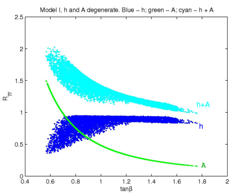
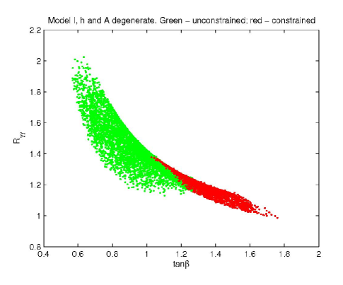
Figure 1: Left panel: $R_{\gamma\gamma}$ as a function of $\tan{\beta}$ for $h$ (blue/black), $A$ (green/gray), and the total observable rate (cyan/light-gray), obtained by summing the rates with intermediate $h$ and $A$, for the unconstrained scenario. Right panel: Total rate for $R_{\gamma\gamma}$ as a function of $\tan{\beta}$ for the constrained (red/black) and unconstrained (green/gray) scenarios.

We have generated a large sample of points in parameter space satisfying all constraints. The results for $R_{\gamma\gamma}$ as a function of $\tan{\beta}$ are presented in Fig. 1 for the unconstrained scenario (left panel) and the constrained scenario (right panel). We note that $R^{h}_{\gamma\gamma}$ lies below unity regardless of $\tan{\beta}$; the wide region of the distributed points reflects the variation as the CP-even mixing angle $\alpha$ is scanned. This result was previously obtained in Ref. sher in the limit of $m_{A}\gg m_{h}$, and in Ref. Barroso:2012wz , allowing for the mixing with the heavier CP-even and CP-odd scalars. In contrast, $R^{A}_{\gamma\gamma}$ increases as $\tan{\beta}$ decreases, as expected, due to the increase in the $At\bar{t}$ coupling [cf. Table 1]. Its value is uniquely determined by $\tan\beta$, as there is no $\alpha$ dependence in the coupling of $A$ to fermions. As a result, the observed rate for $pp\to(h,A)\to\gamma\gamma$ normalized to the corresponding SM rate can take values as large as $2$, for $\tan{\beta}\sim 0.6$. However, constraints from $B$-physics restrict the normalized rate for $pp\to(h,A)\to\gamma\gamma$ to a maximal value of approximately $1.4$, for $\tan{\beta}\sim 1$.

Since $A$ does not couple to $VV$, the $\gamma\gamma$ decays detected in VBF production can only be due to the $h$ intermediate state. The ATLAS and CMS experiments can isolate Higgs signal events with a set of additional criteria (e.g. events with two forward jets with certain transverse momentum cuts and a central jet veto) which they designate as VBF Higgs events. In practice the experimental VBF Higgs events have significant contamination of Higgs events produced by gluon–gluon fusion with the subsequent radiation of two additional jets. Nevertheless, in this work we find it convenient to define a theoretical quantity,

$$R_{\gamma\gamma}^{\rm VBF}=\frac{\sigma(pp\to VV\to h)_{\textrm{2HDM}}\ \textrm{BR}(h\to\gamma\gamma)_{\textrm{2HDM}}}{\sigma(pp\to VV\to h_{\textrm{SM}})\ \textrm{BR}(h_{\textrm{SM}}\to\gamma\gamma)}\,,$$ (4.4)

which would be appropriate if VBF Higgs events could be identified with no contamination. This will prove sufficient for our purposes in this initial study. Likewise, we shall denote $R_{\gamma\gamma}\equiv R^{h}_{\gamma\gamma}+R^{A}_{\gamma\gamma}$ following the definitions given in eq. (2.5).

Fig. 2 shows the allowed region in the $R^{\textrm{VBF}}_{\gamma\gamma}$–$R_{\gamma\gamma}$ plane, for our set of points, for the constrained (red/black) and unconstrained (green/gray) scenarios. In the unconstrained scenario, contrary to what happens for the total $R^{h}_{\gamma\gamma}$, the $h$ intermediate state can induce values of $R^{\textrm{VBF}}_{\gamma\gamma}$ larger than unity. The dispersion of points shows that, in the region of parameter space that we have studied, a comparison between $R^{\textrm{VBF}}_{\gamma\gamma}$ and $R_{\gamma\gamma}$ is unlikely to allow an exclusion of the Type-I 2HDM. Indeed, for $R_{\gamma\gamma}\sim 1.5$, this model allows for any value of $R^{\textrm{VBF}}_{\gamma\gamma}$ between $0.2$ and $1.7$. Only if $R_{\gamma\gamma}\sim 2.0$ can we exclude values of $R^{\textrm{VBF}}_{\gamma\gamma}$ above unity.

In the constrained scenario, $R^{\textrm{VBF}}_{\gamma\gamma}$ is now between $0.7$ and $1.6$, while $R_{\gamma\gamma}$ lies in the range from 1 to 1.4. The allowed values (red/black) clearly show that an enhancement in $R_{\gamma\gamma}$ can only be achieved for $R^{\textrm{VBF}}_{\gamma\gamma}$ close to 1. Conversely, large values of $R^{\textrm{VBF}}_{\gamma\gamma}$ are attained only for a SM-like $R_{\gamma\gamma}$. Naively, it seems puzzling that values of $R_{\gamma\gamma}^{\rm VBF}$ above 1 are possible. After all, this quantity is only sensitive to $h$ production and decay, and we are assuming that the $hVV$ coupling is close to its SM value. A closer examination of the parameter scan reveals that the range of allowed $\alpha$ is rather limited, $-0.9\mathrel{\;{\hbox{\raise 1.50696pt\hbox{$<$}}\kern-3.8889pt\kern-3.8889pt\hbox{\lower 2.79857pt\hbox{$\sim$}}}\;}\sin\alpha\mathrel{\;{\hbox{\raise 1.50696pt\hbox{$<$}}\kern-3.8889pt\kern-3.8889pt\hbox{\lower 2.79857pt\hbox{$\sim$}}}\;}-0.4$. For the values of $\sin\alpha$ close to $-1$, the Type-I couplings of $h$ to fermion pairs are suppressed relative to the corresponding SM couplings. Consequently, the partial width of $h\to b\bar{b}$ is reduced and so the corresponding branching ratio for $h\to\gamma\gamma$ is enhanced relative to its SM value.

Figure 2: Allowed region in the $R^{\textrm{VBF}}_{\gamma\gamma}-R_{\gamma\gamma}$ plane with (red/black) and without (green/gray) the $B$-physics constraints.

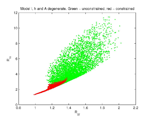
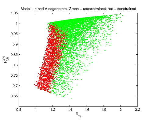
Figure 3: Left panel: Total $R_{\tau\tau}$ ($h$ and $A$ summed) as a function of $R_{\gamma\gamma}$ for the constrained (red/black) and unconstrained (green/gray) scenarios. QCD corrections aside, this figure also holds approximately for $R_{bb}$. Right panel: $R^{\textrm{VH}}_{bb}$ ($h$ and $A$ summed) as a function of $R_{\gamma\gamma}$ for the constrained (red/black) and unconstrained (green/gray) scenarios.

The left panel of Fig. 3 exhibits our results for the inclusive $\tau\tau$ final state, summing over all production mechanisms, for the constrained (red/black) and unconstrained (green/gray) scenarios. Note that both $R_{\tau\tau}$ and $R_{\gamma\gamma}$ include contributions from $h$ and $A$. For the unconstrained scenario, we see that if $R_{\gamma\gamma}\sim 1.5$ then the total $R_{\tau\tau}$ contribution cannot be smaller than about 3.5 and can be as large as 8. When the $B$-physics constraints are included the main difference is again that $R_{\gamma\gamma}\lesssim 1.4$, whereas $R_{\tau\tau}$ lies in a very narrow band heavily dependent on the particular value of $R_{\gamma\gamma}$ but always below about 3. The correlation between the enhanced $\gamma\gamma$ and $\tau\tau$ signals is a noteworthy prediction for this scenario.

There are only very slight differences between $R_{\tau\tau}$ and $R_{bb}$, due to QCD corrections that distinguish the two processes, so the left panel of Fig. 3 would apply as well to a hypothetical measurement of the inclusive $b\bar{b}$ final state. Unfortunately, the detection of $h\to b\bar{b}$ via gluon-gluon production at the LHC is swamped by background and is not possible in the inclusive mode. However, both the ATLAS and CMS collaborations expect some sensitivity to the $b\bar{b}$ final state in the production of the Higgs boson in association with a $W^{\pm}$ or $Z$ (where leptonic decays of the vector bosons can be used to tag the event). The right panel of Fig. 3 exhibits our results for the $b\bar{b}$ final state obtained through $VH$ production, $R^{\textrm{VH}}_{bb}$, with (red/black) and without (green/gray) the $B$-physics constraints. Since $A$ is not produced by this mechanism, we only get a contribution from the SM-like $h$ and the enhancement in the $b\bar{b}$ channel disappears. Furthermore, in the constrained scenario, even an enhancement in $R_{\gamma\gamma}$ corresponds to $R^{\textrm{VH}}_{bb}$ below 1.

4.2 Type-II 2HDM

In the analysis of a mass-degenerate $h$, $A$ pair in the Type-II 2HDM, we have generated a large sample of points satisfying all constraints. We again anticipate that $\sin(\beta-\alpha)$ should be near 1. Applying the same simplified scenario that yielded eq. (4.3) for the Type-I 2HDM, we now obtain

$$R_{ZZ}=\frac{\cos^{2}{\alpha}}{\sin^{2}{\beta}}\sin^{2}{(\alpha-\beta)}\frac{\cos^{2}{\beta}}{\sin^{2}{\alpha}}\,,$$ (4.5)

where we have employed the Type-II couplings of Table 1. Assuming that $\cos(\beta-\alpha)$ is small, we can expand in this small quantity by making use of

$$\frac{\cos^{2}{\alpha}}{\sin^{2}{\beta}}\cdot\frac{\cos^{2}{\beta}}{\sin^{2}{\alpha}}=\left[\frac{\sin(\beta-\alpha)+\cot\beta\cos(\beta-\alpha)}{\sin(\beta-\alpha)-\tan\beta\cos(\beta-\alpha)}\right]^{2}=1+\frac{4\cos(\beta-\alpha)}{\sin 2\beta}+\mathcal{O}\bigl{(}\cos^{2}(\beta-\alpha)\bigr{)}\,.$$ (4.6)

Inserting this result into eq. (4.5) yields

$$\cos(\beta-\alpha)\simeq\tfrac{1}{4}\sin 2\beta(R_{ZZ}-1)\,.$$ (4.7)

In light of eq. (2.6), the assumption that $\cos(\beta-\alpha)$ is small is justified. In our simulation we find that the constraint imposed by eq. (2.6) leads to $\sin{(\beta-\alpha)}>0.996$, which is an even tighter restriction than suggested by eq. (4.7).

Figure 4: $R_{\gamma\gamma}$ as a function of $\tan{\beta}$ for $h$ (blue/black), $A$ (green/gray), and the total observable rate, obtained by summing the rates with intermediate $h$ and $A$ (cyan/light-gray).

Fig. 4 shows $R_{\gamma\gamma}$ as a function of $\tan{\beta}$ for the Type-II 2HDM. Here the $h$ contribution by itself can only reach unity and, as in the Type-I 2HDM, the contribution from $A$ becomes dominant for low $\tan{\beta}$ values. The total $R_{\gamma\gamma}$ can be as large as $3.5$ for $\tan{\beta}\sim 0.7$. Moreover, the requirement that $0.8<R_{ZZ}<1.2$ leads to the exclusion of any point with $\tan{\beta}<0.7$ in our simulation. Because the most important constraint for the Type-II 2HDM is the one from $R_{b}$ and since the charged Higgs mass is varied from 500 to 1000 GeV, $\tan{\beta}$ will not be affected by any further constraints from $B$ physics. This means that all results presented for this Type-II scenario already incorporate all available experimental and theoretical constraints.

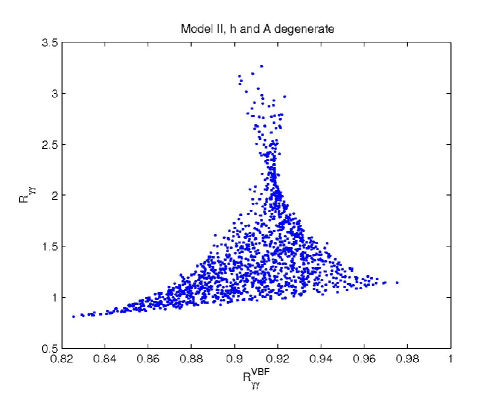
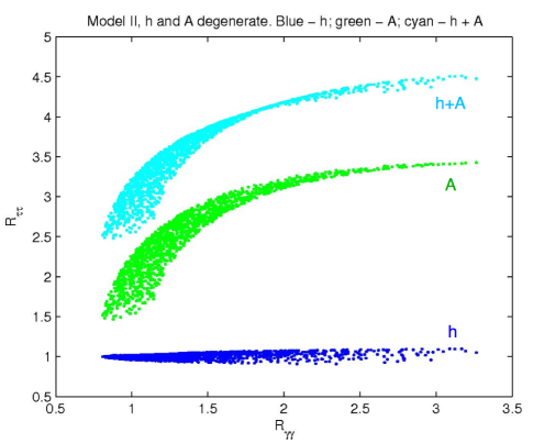
Figure 5: Left panel: Allowed region in the $R^{\textrm{VBF}}_{\gamma\gamma}-R_{\gamma\gamma}$. Right panel: $R_{\tau\tau}$ as a function of $R_{\gamma\gamma}$ for $h$ (blue/black), $A$ (green/gray), and the total observable rate, obtained by summing the rates with intermediate $h$ and $A$ (cyan/light-gray).

The left panel of Fig. 5 exhibits the allowed region in the $R^{\textrm{VBF}}_{\gamma\gamma}$–$R_{\gamma\gamma}$ plane, for our set of points. In stark contrast with the Type-I 2HDM, here $R^{\textrm{VBF}}_{\gamma\gamma}$ is predicted to lie in a rather narrow region close to $0.9$. This is due to the much narrower range obtained for $\sin{(\beta-\alpha)}$, which is constrained to be near 1 in the Type-II scenario, and implies that $\cos\alpha\simeq\sin\beta$ and $\sin\alpha\simeq-\cos\beta$ (i.e. the decoupling limit). Consequently, the Type-II couplings of $h$ to fermion pairs are close to their SM values. It immediately follows that $R^{\textrm{VBF}}_{\gamma\gamma}$ should be close to 1 as indicated by the left panel of in Fig. 5. If the experimental data were to indicate a similar and sizeable enhancement of both $R^{\textrm{VBF}}_{\gamma\gamma}$ and $R_{\gamma\gamma}$, then the $m_{h}\simeq m_{A}$ Type-II scenario would be excluded.

As for $R_{\tau\tau}$, the largest allowed values are less extreme than those of the Type-I model, as can be seen from the right panel of Fig. 5. The lower limit on $R_{\tau\tau}$ depends on the value of $R_{\gamma\gamma}$. For example, for $R_{\gamma\gamma}\sim 1.5$, the total $R_{\tau\tau}$ cannot be smaller than about $3.5$. Notice that the right panel of Fig. 5 shows a rather strong correlation between $R_{\tau\tau}$ and $R_{\gamma\gamma}$ in the Type-II model, while the Type-I model points exhibited in the left panel of Fig. 3 are much more dispersed in the $R_{\gamma\gamma}$–$R_{\tau\tau}$ plane.

5 Degenerate $h$ and $H$

We now turn to the possibility that $m_{h}\simeq m_{H}$. We have generated sets of parameters such that $m_{A}$ and $m_{H^{\pm}}$ lie above 500 GeV. For the case in which $h$ and $H$ are nearly degenerate in mass, we have found that the $S$, $T$, and $U$ constraints force $m_{H^{\pm}}\sim m_{A}$, to within 10%. In this case, an enhancement of the $\gamma\gamma$ signal rate is visible (although not as pronounced) even for values of $\tan{\beta}$ somewhat larger than 2. As a result, we have focused our scan in a $\tan\beta$ regime between $0.5$ and $5$.

5.1 Type-I 2HDM

We begin with the Type-I 2HDM. In the case of a mass degenerate $h$, $A$ pair discussed previously $\sin{(\beta-\alpha)}>0.85$ in both the Type-I and Type-II scenarios, with only a mild correlation with $\tan{\beta}$. In contrast, employing the same simplified scenario that was used in obtaining eq. (4.3), we now obtain

$$R_{ZZ}=R^{h}_{ZZ}+R^{H}_{ZZ}=\frac{\cos^{2}{\alpha}}{\sin^{2}{\beta}}\sin^{2}{(\beta-\alpha)}\frac{\sin^{2}{\beta}}{\cos^{2}{\alpha}}+\frac{\sin^{2}{\alpha}}{\sin^{2}{\beta}}\cos^{2}{(\beta-\alpha)}\frac{\sin^{2}{\beta}}{\sin^{2}{\alpha}}=1,$$ (5.1)

where we have used the couplings of Table 1. In fact, even using all production mechanisms, we find that $R_{ZZ}\sim 1$. Consequently, eq. (2.6) places almost no constraint on the value of $\sin{(\beta-\alpha)}$.

The left panel of Fig. 6 exhibits the allowed region in the $R^{\textrm{VBF}}_{\gamma\gamma}$–$R_{\gamma\gamma}$ plane, for the constrained (red/black) and unconstrained (green/gray) scenarios. The total $R_{\gamma\gamma}$ cannot differ significantly from its SM value. In particular, the maximal allowed $\gamma\gamma$ enhancement is about $1.3$ for the unconstrained scenario, and none of the enhanced values survive after imposing the constraints from $B$ physics. In contrast, $R^{\textrm{VBF}}_{\gamma\gamma}$ can be either very close to vanishing or take values as large as 4 in the unconstrained scenario and as large as 3 in the constrained scenario.

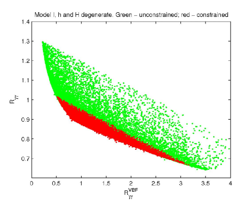
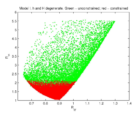
Figure 6: Left panel: Allowed region in the $R^{\textrm{VBF}}_{\gamma\gamma}-R_{\gamma\gamma}$ plane for the constrained (red/black) and unconstrained (green/gray) scenarios. Right panel: Allowed region in the $R_{\gamma\gamma}-R_{\tau\tau}$ plane for the constrained (red/black) and unconstrained (green/gray) scenarios.

The possibility of an enhanced $R^{\textrm{VBF}}_{\gamma\gamma}$ arises due to the fact that $\alpha$ is not especially constrained by the requirement of eq. (2.6). In particular, the limit of $\sin\alpha=\pm 1$ [$\sin\alpha=0$] corresponds to the fermiophobic limit for $h$ [$H$]. In this limit, the dominant fermiophobic Higgs boson decay channels are $WW^{*}$ and $ZZ^{*}$, in which case we expect the corresponding branching ratio into $\gamma\gamma$ (which should be approximately given by the ratio of the $\gamma\gamma$ and $WW^{*}$ partial widths) to be enhanced by a factor of roughly 5 relative to its value in the SM. Thus, even though the VBF production cross-section is roughly given by its SM value, it is not surprising that one can achieve values of $R^{\textrm{VBF}}_{\gamma\gamma}$ as large as shown in the left panel of Fig. 6. Moreover, one also expects a reduced value of $R_{\gamma\gamma}$, since in the fermiophobic limit the size of the gluon-gluon fusion cross section (which depends on the coupling of the Higgs boson to $t\bar{t}$) is significantly suppressed. Assuming that the VBF production mechanism now dominates, it follows that the Higgs production cross-section has been reduced by roughly a factor of 10 relative to the SM Higgs production cross-section via gluon-gluon fusion. This reduction factor of 10 cannot be completely compensated by an increase in the Higgs to $\gamma\gamma$ branching ratio, which implies that $R_{\gamma\gamma}<1$ in the fermiophobic regime, as shown in the left panel of Fig. 6.

The right panel of Fig. 6 exhibits $R_{\tau\tau}$ as a function of $R_{\gamma\gamma}$. It is interesting to compare the Type-I scenarios exhibited by the left panel of Fig. 3, which holds for the case of a mass-degenerate $h$, $A$ pair, with the right panel of Fig. 6, which holds for the case of a mass-degenerate $h$, $H$ pair. In contrast to the former scenario, where $R_{\gamma\gamma}$ could reach about $2$ while $R_{\tau\tau}$ could reach $11$, in the present scenario $R_{\gamma\gamma}$ can be at most $1.3$ while $R_{\tau\tau}$ is smaller than $5.5$. Nevertheless, the lower bound on $R_{\tau\tau}$ for $R_{\gamma\gamma}>1.1$ is more stringent in the latter scenario than in the former. Indeed, when $m_{h}\simeq m_{A}$ and $R_{\gamma\gamma}=1.2$, we predict $R_{\tau\tau}>2$, whereas when $m_{h}\simeq m_{H}$ and $R_{\gamma\gamma}=1.2$, we predict $R_{\tau\tau}>3.5$. Again, in the constrained scenario, $R_{\gamma\gamma}$ has to be below $1$ while $R_{\tau\tau}$ cannot be above $2$. The constrained scenario makes a very strong prediction: $R_{\gamma\gamma}$ has to be SM-like or smaller, whereas $R_{\tau\tau}$ must be above the SM prediction.

5.2 Type-II 2HDM

In this case there is a strong correlation between $\sin{(\beta-\alpha)}$ and $\tan{\beta}$. Employing the same simplified scenario that was used in obtaining eq. (4.3) and using the couplings of Table 1, we now obtain

$$R_{ZZ}=R^{h}_{ZZ}+R^{H}_{ZZ}=\frac{\cos^{2}{\alpha}}{\sin^{2}{\beta}}\sin^{2}{(\beta-\alpha)}\frac{\cos^{2}{\beta}}{\sin^{2}{\alpha}}+\frac{\sin^{2}{\alpha}}{\sin^{2}{\beta}}\cos^{2}{(\beta-\alpha)}\frac{\cos^{2}{\beta}}{\cos^{2}{\alpha}}\,.$$ (5.2)

The above result can be expressed directly in terms of $\tan\beta$ and $\sin(\beta-\alpha)$ by employing eqs. (4.1) and (4.2),

$$R_{ZZ}=\frac{[\tan^{2}\beta+\cot^{2}\beta+2]c^{2}_{\beta-\alpha}s^{2}_{\beta-\alpha}+[\tan\beta(c^{2}_{\beta-\alpha}-s^{2}_{\beta-\alpha})-2c_{\beta-\alpha}s_{\beta-\alpha}]^{2}}{[\tan\beta(c^{2}_{\beta-\alpha}-s^{2}_{\beta-\alpha})-(1-\tan^{2}\beta)c_{\beta-\alpha}s_{\beta-\alpha}]^{2}}\,,$$ (5.3)

where $c_{\beta-\alpha}\equiv\cos(\beta-\alpha)$ and $s_{\beta-\alpha}\equiv\sin(\beta-\alpha)$. Thus, eqs. (2.6) and (5.3) impose a complicated constraint in the $\sin(\beta-\alpha)$–$\tan\beta$ plane. For example, for model points where $0.8<R_{\gamma\gamma}<1.5$, the allowed regions in the $\sin(\beta-\alpha)$–$\tan\beta$ plane are shown in the left panel of Fig. 7. The uppermost (lowermost) two bands correspond to a dominant $h$ ($H$) contribution to $R_{\gamma\gamma}$. In the band around $\sin{(\beta-\alpha)}\sim 1$, $h$ is gaugephilic and $H$ is gaugephobic. In the second band below, the contribution of $h$ to $R_{\gamma\gamma}$ is still dominant, with a small contribution by $H$. In the next band, the roles of $h$ and $H$ are reversed, and in the band around $\sin{(\beta-\alpha)}\sim 0$, $H$ is gaugephilic while $h$ is gaugephobic.

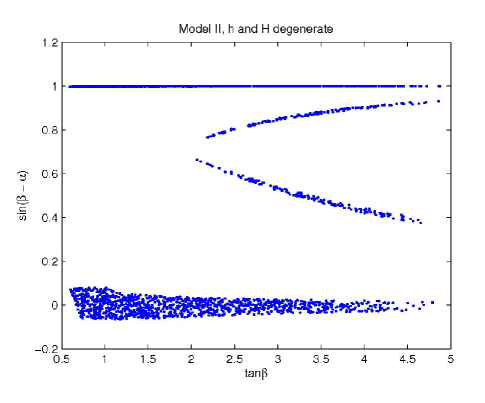
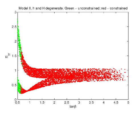
Figure 7: Left panel: Values obtained in the $\tan{\beta}-\sin{(\beta-\alpha)}$ plane for the points generated, which satisfy $0.8<R_{\gamma\gamma}<1.5$. Right panel: Values for $R_{\gamma\gamma}$ as a function of $\tan{\beta}$ for the constrained (red/black) and unconstrained (green/gray) scenarios.

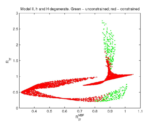
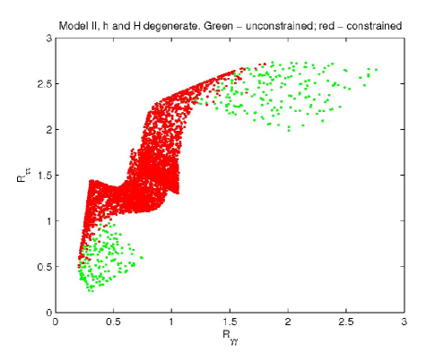
Figure 8: Left panel: Allowed region in the $R^{\textrm{VBF}}_{\gamma\gamma}$–$R_{\gamma\gamma}$ plane for the constrained (red/black) and unconstrained (green/gray) scenarios. Right panel: Allowed region in the $R_{\gamma\gamma}$–$R_{\tau\tau}$ plane for the constrained (red/black) and unconstrained (green/gray) scenarios.

The band structure exhibited in the left panel of Fig. 7 impacts the $R_{\gamma\gamma}$ dependence on $\tan{\beta}$, as shown in the right panel of Fig. 7. The generated set of points are plotted in the $R^{\textrm{VBF}}_{\gamma\gamma}$–$R_{\gamma\gamma}$ plane in the left panel of Fig. 8, whereas the allowed regions in the $R_{\gamma\gamma}$–$R_{\tau\tau}$ plane is shown in the right panel of Fig. 8 for the constrained (red/black) and unconstrained (green/gray) scenarios. It is instructive to compare the $m_{h}\simeq m_{H}$ type-II model analyzed in this section with the $m_{h}\simeq m_{A}$ type-II model examined in Section 4.2. Comparing left panels of Fig. 5 and Fig. 8, we see that the former scenario allows for larger values of $R_{\gamma\gamma}$. In contrast, the values of $R^{\textrm{VBF}}_{\gamma\gamma}$ are very constrained in the former scenario, while in the latter scenario these values can range from $0$ to $1.1$. Comparing the right panels of Fig. 5 and Fig. 8, we see that $2.5<R_{\tau\tau}<4.5$ in the case of $m_{h}=m_{A}$, whereas $0.2<R_{\tau\tau}<2.7$ in the case of $m_{h}=m_{H}$.

Once the constraints of $B$ physics are applied, the most striking difference from the results presented above is that the value of $R_{\gamma\gamma}$ in the constrained scenario must be below $1.5$. The allowed ranges of $R^{\textrm{VBF}}_{\gamma\gamma}$ and $R_{\tau\tau}$ are quite narrow. However, a definite measurement of $R_{\gamma\gamma}=1.5$ would force $R_{\tau\tau}\approx 2.5$. It is also interesting to compare the $m_{h}\simeq m_{H}$ Type-II model analyzed here with the $m_{h}\simeq m_{H}$ Type-I model examined in Section 5.1. Here the enhancement in $R_{\gamma\gamma}$ can be larger, whereas the upper bounds on the enhancements in $R^{\textrm{VBF}}_{\gamma\gamma}$ and $R_{\tau\tau}$ are somewhat reduced. In summary, it is more difficult to generate an enhancement of $R_{\gamma\gamma}$ in the $m_{h}\simeq m_{H}$ case as compared to the $m_{h}\simeq m_{A}$ case. On the other hand, the corresponding enhancement of $R_{\tau\tau}$ is also reduced.

6 Degenerate $H$ and $A$

Now we turn to the case where $m_{h}<m_{H}\simeq m_{A}\simeq$ 125 GeV. In the previous cases we have studied, we could keep $m_{H^{\pm}}>500\,\textrm{GeV}$. In this case, there are no points with $m_{H^{\pm}}>200\,\textrm{GeV}$ that survive the constraints coming from boundedness from below, unitarity, and precision electroweak measurements. Since the constraints from $b\to s\gamma$ imply $m_{H^{\pm}}>360\,\textrm{GeV}$ in the Type-II 2HDM, the whole of parameter space with $m_{H}\simeq m_{A}\simeq$ 125 GeV is excluded in the Type-II model. Thus we examine the $m_{A}\simeq m_{H}$ scenario in Type-I 2HDM, keeping $0.5<\tan{\beta}<5$.

Figure 9: Values obtained in the $\tan{\beta}$–$\sin{(\beta-\alpha)}$ plane for the points generated for the constrained (red/black) and unconstrained (green/gray) scenarios.

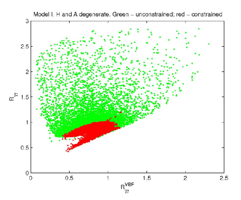
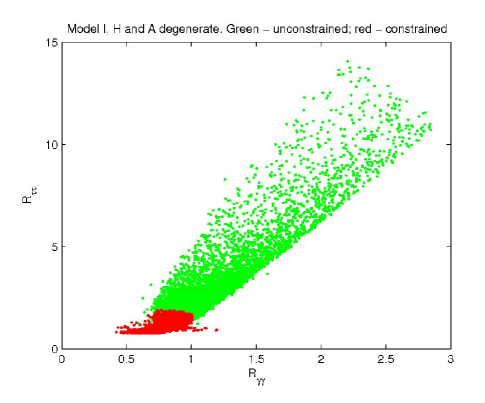
Figure 10: Left panel: Allowed region in the $R^{\textrm{VBF}}_{\gamma\gamma}$–$R_{\gamma\gamma}$ plane for the constrained (red/black) and unconstrained (green/gray) scenarios. Right panel: Allowed region in the $R_{\gamma\gamma}$–$R_{\tau\tau}$ plane for the constrained (red/black) and unconstrained (green/gray) scenarios.

If $m_{h}<m_{H}/2$, then the branching ratio for $H\to hh$ would be close to one, greatly suppressing the $ZZ^{*}$ signal (to which $A$ cannot contribute). As a result, we shall assume that $m_{h}>m_{H}/2$. In particular, we examine the mass range $65\,\textrm{GeV}<m_{h}<110\,\textrm{GeV}$. Such a low-mass $h$ could have been produced at LEP via the $ZZh$ vertex, which is suppressed by a factor of $\sin{(\beta-\alpha)}$ in the 2HDM. The model points surviving the LEP constraints mssmhiggs , in which eq. (2.6) is satisfied due to $H$ production and decay, are shown in the $\tan{\beta}$–$\sin{(\beta-\alpha)}$ plane of Fig. 9 for the constrained (red/black) and unconstrained (green/gray) scenarios. Note that because the charged Higgs boson in now forced to be light, the $B$-physics constraints imply a value of $\tan\beta$ above $2$. As expected, the points are centered around $\sin{(\beta-\alpha)}=0$, but values as large as $|\sin{(\beta-\alpha)}|\sim 0.5$ are possible.

The generated set of points are plotted in the $R^{\textrm{VBF}}_{\gamma\gamma}$–$R_{\gamma\gamma}$ plane in the left panel of Fig. 10 for the constrained (red/black) and unconstrained (green/gray) scenarios. Contrary to the previous scenarios with $m_{h}\simeq m_{A}$ or $m_{h}\simeq m_{H}$ in the Type-I model, both $R^{\textrm{VBF}}_{\gamma\gamma}$ and $R_{\gamma\gamma}$ now have a much wider range of variation and can reach $2.3$ simultaneously. However, in the constrained scenario the $R^{\textrm{VBF}}_{\gamma\gamma}$ values drop to a maximum of around $1.2$ while $R_{\gamma\gamma}$ drops to a maximum close to $1$. The allowed region in the $R_{\gamma\gamma}$–$R_{\tau\tau}$ plane for this set of points is shown in the right panel of Fig. 10. We note that the constrained scenario lives in a region very close to the SM prediction.

7 Degenerate $h$, $H$ and $A$

In this section we discuss the case where $m_{h}\simeq m_{H}\simeq m_{A}\simeq 125$ GeV, i.e. all three neutral scalars are nearly mass-degenerate. As in the previous scenario with $m_{H}\simeq m_{A}$, the electroweak precision constraints force the charged Higgs to be light (below approximately 200 GeV). Hence, due to the $b\to s\gamma$ bound on the charged Higgs mass, this scenario is ruled out in the Type-II 2HDM.

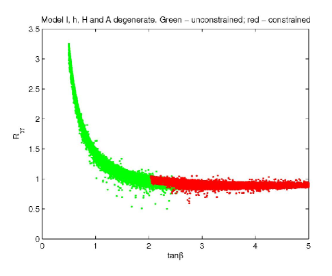
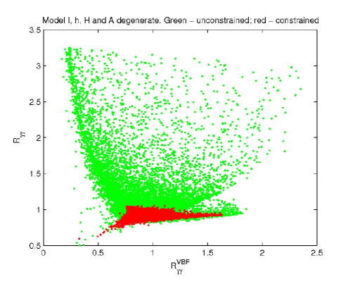
Figure 11: Left panel: Total $R_{\gamma\gamma}$ ($h$, $H$ and $A$ summed) as a function of $\tan\beta$ for the constrained (red/black) and unconstrained (green/gray) scenarios. Right panel: Allowed region in the $R^{\textrm{VBF}}_{\gamma\gamma}-R_{\gamma\gamma}$ plane for the constrained (red/black) and unconstrained (green/gray) scenarios.

In the left panel of Fig. 11 we present the total $R_{\gamma\gamma}$, with $h$, $H$ and $A$ summed, as a function of $\tan\beta$ for the constrained (red/black) and unconstrained (green/gray) scenarios in the Type-I 2HDM. This scenario does not differ much from the previous one where again only Type-I was allowed. In particular, when all constraints are imposed, the maximum value of $R_{\gamma\gamma}$ has to lie very close to $1$. In the right panel of Fig. 11 we present the allowed region in the $R^{\textrm{VBF}}_{\gamma\gamma}$–$R_{\gamma\gamma}$ plane for the constrained (red/black) and unconstrained (green/gray) scenarios. If we now compare this scenario with the three previous ones we conclude that the differences are not that striking, especially in the constrained case: $R^{\textrm{VBF}}_{\gamma\gamma}$ can be larger than the SM value reaching 1.7 while $R_{\gamma\gamma}$ has to be very close to the value predicted by the SM. However, a large value of $R^{\textrm{VBF}}_{\gamma\gamma}=1.7$ and $R_{\gamma\gamma}=1$ is only allowed in the present scenario and in the Type-I 2HDM with $m_{H}\simeq m_{h}$. In fact, the difference between these two scenarios is primarily due to the theoretical and experimental constraints: when $m_{H}\simeq m_{h}$ a nearly-fermiophobic scenario is allowed with values of $R^{\textrm{VBF}}_{\gamma\gamma}$ reaching 3. In contrast, when all the neutral Higgs masses are degenerate the fermiophobic limit cannot be attained, and $R^{\textrm{VBF}}_{\gamma\gamma}$ reaches a maximum value of $1.7$.

8 Conclusions

In this paper, we have addressed the possibility that an enhanced $\gamma\gamma$ signal in Higgs production at the LHC (under the assumption of a SM-like $ZZ\to 4~{}{\rm leptons}$ signal) can be explained in the context of the 2HDM by a pair of nearly mass-degenerate neutral Higgs bosons with a mass around 125 GeV. To analyze this scenario, we have examined the softly broken $\mathbb{Z}_{2}$-symmetric and CP-conserving 2HDM with either Type-I or Type-II Higgs-fermion Yukawa couplings. We have scanned the resulting 2HDM parameter spaces, subject to the constraints of all known experimental observables (excluding the recently observed anomaly of $\overline{B}\to D^{(*)}\tau^{-}\overline{\nu}_{\tau}$ by the BaBar collaboration, which has not yet been confirmed by the Belle collaboration).

We find that, in the degenerate mass scenario, it is only possible to produce an enhanced $\gamma\gamma$ signal in a region of parameter space where $\tan\beta$ is near 1. This result immediately implies that it is not possible to realize such a scenario in the MSSM, since the additional constraints imposed by supersymmetry combined with the LEP search for the Higgs bosons of the MSSM rule out values of $\tan\beta$ below about 2 mssmhiggs .

In particular, we have demonstrated that an enhanced $\gamma\gamma$ signal could be due to a nearly mass-degenerate $h$, $A$ pair or $h$, $H$ pair. (In the case where $H$ and $A$ are nearly mass-degenerate, it is much more difficult to achieve a significant enhancement in the $\gamma\gamma$ signal subject to all the experimental constraints.) In the parameter region corresponding to an enhanced $\gamma\gamma$ signal, we generically expect an enhanced inclusive $\tau^{+}\tau^{-}$ signal, due to the contribution of the second mass-degenerate Higgs state in addition to the $\tau^{+}\tau^{-}$ signal produced by the SM-like Higgs state.

The absence of an enhanced $\tau^{+}\tau^{-}$ signal would be strong evidence against the scenario proposed in this paper. However, if both a $\gamma\gamma$ and $\tau^{+}\tau^{-}$ enhancement are confirmed, then one can probe the nature of the Higgs–fermion Yukawa couplings by distinguishing $\gamma\gamma$ signal events that arise from vector boson fusion (VBF). For example, we find that an enhanced VBF $\gamma\gamma$ rate is possible in Type-I models but is not possible in Type-II models.

Of course, ultimately the verification of the mass-degenerate scenario would require the observation of two separate scalar states. As we do not expect these states to be exactly mass-degenerate, it is possible that the inherent experimental mass resolutions of the ATLAS and CMS experiments could eventually be sensitive to the presence of two (or more) approximately mass-degenerate scalar states. In particular, in the mass-degenerate scenarios studied in this paper, the $\gamma\gamma$ signal is a consequence of the production and decay of both mass-degenerate Higgs bosons, whereas the $ZZ^{*}\to 4$ lepton signal derives primarily from the production and decay of a single Higgs boson with SM-like couplings to vector boson pairs. Thus, an observation of slightly different invariant masses in the $\gamma\gamma$ and $ZZ^{*}\to 4$ lepton channels would be strong evidence that a scenario similar to the ones examined in this paper is realized in nature.