Grid-based exploration of cosmological parameter space with Snake

Abstract

We present a fully parallelized grid-based parameter estimation algorithm for investigating multidimensional likelihoods called Snake, and apply it to cosmological parameter estimation. The basic idea is to map out the likelihood grid-cell by grid-cell according to decreasing likelihood, and stop when a certain threshold has been reached. This approach improves vastly on the “curse of dimensionality” problem plaguing standard grid-based parameter estimation simply by disregarding grid-cells with negligible likelihood. The main advantages of this method compared to standard Metropolis-Hastings MCMC methods include 1) trivial extraction of arbitrary conditional distributions; 2) direct access to Bayesian evidences; 3) better sampling of the tails of the distribution; and 4) nearly perfect parallelization scaling. The main disadvantage is, as in the case of brute-force grid-based evaluation, a dependency on the number of parameters, $N_{\textrm{par}}$. One of the main goals of the present paper is to determine how large $N_{\textrm{par}}$ can be, while still maintaining reasonable computational efficiency; we find that $N_{\textrm{par}}=12$ is well within the capabilities of the method. The performance of the code is tested by comparing cosmological parameters estimated using Snake and the WMAP-7 data with those obtained using CosmoMC, the current standard code in the field. We find fully consistent results, with similar computational expenses, but shorter wall time due to the perfect parallelization scheme.

1. Introduction

Cosmological models are described in terms of a modest number of cosmological parameters that reflect the underlying physical processes of the universe. These are today routinely measured by experiments such as WMAP (Jarosik et al., 2011), Planck (2011) and the Sloan Digital Sky Survey (York et al., 2000) through likelihood techniques.

The most popular parameter estimation algorithm in the cosmology community to date is the CosmoMC package (Lewis & Bridle, 2002), which maps out the cosmological parameter space using a Metropolis-Hastings Markov Chain Monte-Carlo (MCMC) sampler. The computational cost of this method is almost exclusively determined by the external evaluation of the likelihood, which typically takes a few seconds per evalution; the expense of the internal book-keeping operation is completely negligible compared to this. A complete analysis of current data sets typically requires $\mathcal{O}(10^{5})$ evaluations, resulting in an overall computational cost of 100-10,000 CPU hours, depending on the particular problem.

This process can be sped up in two fundamentally different ways, namely either by reducing the cost per likelihood evaluation, or by reducing the number of likelihood evaluations required, and both cases have already been explored extensively in the literature. Examples of the former include CMBFit (Sandvik et al., 2004), PICO (Fendt & Wandelt, 2007), COSMONET (Auld et al., 2007), sparse grids (Frommert et al., 2010) and PkANN (Agarwal et al., 2012), all of which essentially build up a library of known cosmological models given a set of parameters, and interpolate within this library using some statistical method. Examples of the latter include MultiNest (Feroz et al., 2009) and APS (Daniel et al., 2012), both of which reduce the number of likelihood evalutions through more efficient sampling algorithms than the Metropolis-Hastings sampler.

In this paper, we present an algorithm that falls in the last category, aiming to reduce the total number of likelihood evaluations rather than the cost per evaluation. The initial idea of this paper is based on the following reasoning: If the problem under consideration involved only a one-dimensional likelihood, the mapping algorithm of choice would be obvious – one would simply evaluate the likelihood over a one-dimensional grid. The resulting function is both easier to work with than a set of samples, as produced by a MCMC algorithm, and more accurate. Furthermore, it generally requires fewer evaluations, because whereas an MCMC approach builds up the shape of the distribution by counting how many samples fall in a given parameter range (“bin”), the direct approach only needs to evaluate the likelihood in a given bin once. In other words, the MCMC approach spends most of the time evaluating the same likelihood points over and over again, which can give the direct evaluation approach a computational edge.

The vast majority of two-dimensional likelihoods are also mapped by grid methods rather than MCMC methods, while for three or four dimensions, the preferred approach is not clear. However, for higher dimensions, virtually all cases are so far handled by MCMC methods. At this stage, the so-called “curse of dimensionality” becomes highly relevant, as the number of likelihood evaluations depends exponentially on the number of dimensions. For instance, computing 100 grid points in each of five dimensions requires $100^{5}$ evaluation, which is generally far too many for most problems.

However, in this paper we point out that this is not necessarily true. The point is simply that the vast majority of the high-dimensionality volume typically has negligible likelihood, and therefore does not need to be evaluated in the first place. The trick is to figure out which grid cells are relevant and which are not. If this can be done both efficiently and robustly, all the useful properties of normal grids are retained, and computational cost is not compromised. Further, by virtue of not being a Markov chain, the algorithm parallelizes trivially, leading to shorter overall computational wall time, which is often even more critical for a given analysis problem than the total CPU time.

2. The Snake algorithm

2.1. Algorithm

The Snake algorithm is very simple, and easily explained in terms of a few basic steps. To do so succinctly, it is useful to first define some terminology:

The grid

The Snake algorithm operates in a virtual grid defined by an origo, $\theta_{0}$ and a grid cell size, $\Delta\theta$, for each parameter. All points in parameter space are referred to and stored as an $N_{\textrm{par}}$ array on the form $\theta_{0}+\mathbf{k}\Delta\theta$, where $\mathbf{k}$ is an integer vector describing the multidimensional bin number.

The surface

Each point in the grid can be assigned to one of three groups, namely external, internal and surface points. External points are those that have not yet been considered; internal points are those for which likelihoods have been computed for both the point itself and all its neighbors; surface points are points that have been considered, but have at least one unexplored neighbor.

The repository

Each considered parameter point is stored as an object in a data structure called the repository. This is a two-dimensional dynamic list in which each row defines one grid point, and contains $\mathbf{k}$, the likelihood value, the locations of its neighbors in the linked list, and a logical flag specifying whether the point is currently on the surface.

Given these definitions, the Snake algorithm may be summarized as follows:

1. Initialization: Insert $\theta_{0}$ into the repository.

2. Evaluation: Consider the surface point with the highest likelihood, $\mathbf{h}$, and randomly pick one of its unexplored neighbors, $\mathbf{h}+\Delta$. Evaluate $\mathcal{L}(\theta_{\mathbf{h}+\Delta})$.

3. Surface update: If $\mathbf{h}$ has no more unexplored neighbors, set its surface flag to false. Insert $\mathbf{h}+\Delta$ into the repository; if all its neghbors have already been explored set its surface flag to false.

4. Convergence check: If $\log\mathcal{L}(\theta_{\textrm{best-fit}})-\log\mathcal{L}(\theta_{i})$ is smaller than a predefined threshold for all surface points, $i$, then exit. If not, go to (2).

This stepping procedure leads to two distinct phases. First there is a burn-in period in which the solver performs a greedy maximum-likelihood search. Then, once the maximum has been found, the area around the peak is investigated such that the surface grows outwards according to the underlying likelihood distribution, until the threshold is reached. A larger threshold ensures that the tails are investigated more closely, but also means that more evaluations need to the performed which is computationally expensive, thus the threshold should be kept low, though still making sure the edges are properly investigated.

The likelihood evaluation is by far the most time consuming part in cosmological evaluations. This implies that the Snake algorithm can be very efficiently parallelized. In the current implementation we have adopted a master–slave parallelization strategy, in which one processor maintains the repository, and the remaining processors only perform likelihood evaluations for parameters provided by the master. This ensures both a simple implementation as well as close to perfect speed-up; after only a few initial iterations there are always more than enough available surface points to keep all processors occupied. Moreover, the communication between the master and slave is minimal, consisting only of a parameter multiplet and a likelihood return value.

As should be clear from the above, Snake is algorithmically trivial; this is nothing but an old-fashioned likelihood grid evaluation. The only somewhat intricate part is to implement efficient book-keeping, which is necessary in order to maintain computational efficiency as the number of data elements, $V$, in the repository increases. For this purpose, we implement dictionaries, based on the C++ standard map template. These maps store the combination of two values, the key and the mapped value, and enable access to the mapped value by using the corresponding key in constant time, as opposed to $\mathcal{O}(V)$ for unsorted lists or $\mathcal{O}(\log V)$ for sorted lists.

Two such maps are implemented for the master in Snake. The first is for keeping track of which points in parameter space correspond to which iteration, and is used to check if the neighbors of the current point have already been visited, and if so returns their iteration index. The second map keeps track of which likelihood value corresponds to which iteration and is sorted according to descending likelihood such that the first point on the list will always be that with the highest likelihood, and therefore the index of the maximum likelihood on the surface is just the mapped value at the top of the map. When a point becomes an interior point the corresponding entries are removed from the two maps in order to keep these as short as possible and to avoid getting stuck at the overall maximum likelihood.

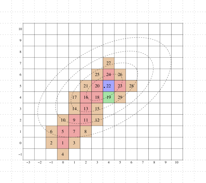
Figure 1.— A snapshot of a made up likelihood distribution after 29 iterations illustrating the repository of Snake. Beige boxes are surface points, red are internal points, blue is the overall maximum likelihood, and green is the maximum likelihood on the surface.

Table 12D book repository

$i$	$\mathbf{k}$		$\mathcal{L}$	Ind				Surface
	x	y		x:-1	x:+1	y:-1	y:+1
1	0	0	0.005	2	3	4	5	F
2	-1	0	0.003		1		6	T
3	1	0	0.002	1			7	T
4	0	-1	0.001				1	T
5	0	1	0.10	6	7	1	10	F
6	-1	1	0.05		5	2		T
7	1	1	0.15	5	8	3	9	F
8	2	1	0.10	7			11	T
22	4	5	0.95	20	23	19	24	F
23	5	5	0.75	22	28	29	26	F
24	4	6	0.70	25	26	22	27	F
25	3	6	0.60		24	20		T
26	5	6	0.70	24		23		T
27	4	7	0.45			24		T
28	6	5	0.55	23				T
29	5	4	0.55	19			23	T

2.2. Walk-through of two-dimensional example

Before testing the algorithm on realistic cases, it is useful to walk through it step-by-step for a simple case, to gain some intuition for its behaviour. In this section, we therefore first consider the small two-dimensional example illustrated in Figure 1 and Table 1. The unknown distribution to be mapped is marked in Figure 1 by dashed lines, corresponding to 1, 2 and $3\sigma$ contours, and the threshold to be reached is defined as the $3\sigma$ contour.

First, we initialize the code at $(0,0)$, which in this case happened to lie slightly below and to the left of the maximum-likelihood point. We evaluate the likelihood, and insert this point into the first row of the repository (Table 1). At this stage, the first four columns are finalized, the surface flag is set to true, and none of the neighbor indices (indicated by the ind array of length $2N_{\textrm{par}}$) are set, indicating that no neighbors have been evaluated yet.

Second, as specified by the algorithm we now find the surface point with the highest likelihood, which of course is the point just added. We select one of its neighbors, which in this case happened to be $(-1,0)$. We evaluate its likelihood, and insert this new point into the second row of the repository. We update the neighbor indices of both this new point and the original point to point to each others main index. We then repeat this process over and over again, adding more and more points to the repository, until the smallest difference between the likelihood of the overall maximum-likelihood point and that of any point on the surface is larger than a pre-defined threshold.

Table 1 gives a snap-shot of the repository (parameters, likelihood, current status of the ind array and the surface flag) at iteration number 29, matching the illustration seen in Figure 1. The beige boxes correspond to the points in parameter space which lie on the surface, red boxes are interior points and the blue box corresponds to the overall maximum likelihood. The green box is the parameter point on the surface with the highest likelihood and will be the start point for the next iteration. The numbers inside the boxes correspond to the iteration index, thus the path Snake takes to reach the maximum likelihood can be see, as well as the relation between neighbors and the values of the first and last eight points quoted in the ind array in Table 1. Iterations which have all ind columns filled have their surface flag set to false and the point no longer exists in the maps. The process continues until all boxes touching the $3\sigma$ contour have turned red, after which the surface lies fully below the threshold.

2.3. Exploration of double-peaked likelihood

A second illustration of how Snake investigates parameter space is given by the double-peaked 2-dimensional likelihood

$$\mathcal{L}=A_{1}\textrm{e}^{\frac{1}{2}(\boldsymbol{x}-\boldsymbol{\mu_{1}})^{T}C_{1}^{-1}(\boldsymbol{x}-\boldsymbol{\mu_{1}})}+A_{2}\textrm{e}^{\frac{1}{2}(\boldsymbol{x}-\boldsymbol{\mu_{2}})^{T}C_{2}^{-1}(\boldsymbol{x}-\boldsymbol{\mu_{2}})},$$ (1)

where $\boldsymbol{x}$ is the 2-dimensional parameter vector, $A_{1}$ and $A_{2}$ are the peak amplitudes, $C_{1}$ and $C_{2}$ the corresponding covariance matrices and $\boldsymbol{\mu_{1}}$ and $\boldsymbol{\mu_{2}}$ the vectors of the means.

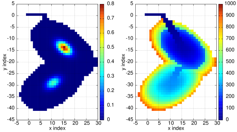
Figure 2.— Two-dimensional illustration of Snake’s sampling method. Left: The (unnormalized) target likelihood. Right: The path Snake takes through parameter space. It finds the closest peak, investigates the area around this peak, discovers the second peak, investigates the area around this one, and finally explores the joint boundary of both peaks.

The leftmost plot of Figure 2 shows a likelihood distribution that can be described by this equation for a particular set of covariance matrices and means. The path Snake takes in the two-dimensional parameter space is shown in the rightmost plot of Figure 2 and as can be seen Snake quickly finds the maximum likelihood of the closest peak, and then proceeds by investigating the area around this peak by visiting neighbors of the surface point with highest likelihood. When the likelihood being investigated falls to the value corresponding to the intersection of the two peaks Snake makes its way to the second peak, and continues by investigating the area around this peak in the same manner as the first peak. Once Snake returns to the likelihood equal to that at the intersection it will investigate the points around both peaks until the desired threshold is reached.

Note that if the two peaks had been so far apart that the likelihood at the intersection fell below the threshold cutoff the second peak would remain undiscovered. This problem can be solved in the same way as for standard Metropolis-Hasting samplers: Run several Snakes in parallel with different initial positions. Once two independent Snakes touch for the first time, merge the repositories and the CPU working groups into one master-slave organization.

3. Accuracy and efficiency with increasing dimensionality

The main outstanding question regarding the Snake algorithm is how well it scales with the number of dimensions in terms of efficiency. To study this question quantitatively, we consider a correlated Gaussian likelihood on the form

$$\mathcal{L}=\textrm{e}^{\frac{1}{2}(\boldsymbol{x}-\boldsymbol{\mu})^{T}C^{-1}(\boldsymbol{x}-\boldsymbol{\mu})},$$ (2)

where $\boldsymbol{x}$, $C$ and $\boldsymbol{\mu}$ are the multidimensional parameter vector, covariance matrix and vector of means, respectively. Both the mean and standard deviation of dimension number $i$ are arbitrarily chosen to be $i$.

Table 2Cosmological parameters

Parameter	CosmoMC		Snake		Shift in $\sigma$
$\Omega_{b}h^{2}$	0.02252	${}^{+0.00055}_{-0.00056}$	0.02252	${}^{+0.00057}_{-0.00056}$	0
$\Omega_{DM}h^{2}$	0.1110	${}^{+0.0055}_{-0.0054}$	0.1107	${}^{+0.0055}_{-0.0054}$	0.06
$\theta$	1.039	$\pm 0.003$	1.039	$\pm 0.003$	0
$\tau$	0.08849	${}^{+0.00632}_{-0.00754}$	0.08758	${}^{+0.01558}_{-0.01426}$	0.08
$n_{s}$	0.9682	${}^{+0.0138}_{-0.0136}$	0.9681	${}^{+0.0139}_{-0.0138}$	0.07
$\textrm{log}[10^{10}A_{s}]$	3.082	${}^{+0.034}_{-0.035}$	3.080	$\pm$ 0.035	0.06

Note. — Comparison of best-fit parameters derived by CosmoMC and Snake from the 7-year WMAP data.

Our goal is now to map out this distribution in $N_{\textrm{par}}$ dimensions, and determine the maximum number of dimensions that can be probed with high accuracy using reasonable computational resources. To do so, we impose a limit on the number of likelihood evaluations of $N=10^{6}$, a typical number for modern cosmological analyses. The grid cell width in dimension $i$ is chosen to be $8i\times N^{1/N_{\textrm{par}}}$, corresponding to distributing the $N$ evaluations roughly over a grid covering roughly $-4\sigma$ to $+4\sigma$ in each of the $N_{\textrm{par}}$ dimensions. (Of course, the actual shape probed by Snake will not be a rectangular grid, but rather conform to the shape of the underlying distribution.) We then run the algorithm for increasing $N_{\textrm{par}}$, and compare the resulting marginals to the known analytic input marginals; once the combined error in the derived mean or standard deviation is larger than $0.1\sigma$, we consider the algorithm to have broken down as a result of the sparse sampling of the underlying distribution.

In Figure 3 we plot the combined mean and standard deviation errors averaged over the number of dimensions, $N_{\textrm{par}}$, as a function of $N_{\textrm{par}}$. Here we clearly see that for $N_{\textrm{par}}<12$, the algorithm recovers the true distribution with high accuracy. Of course, given more computational resources these errors can be decreased arbitrarily, but since the cost faces an exponential growth with increasing $N_{\textrm{par}}$, it seems reasonable to define the operational range for Snake to be $N_{\textrm{par}}\leq 12-15$.

Figure 3.— Combined mean and standard deviation errors averaged over number of dimensions (solid) showing the $0.1\sigma$ cuttoff (dashed).

4. 7-year WMAP likelihood analysis

4.1. Parameter estimation

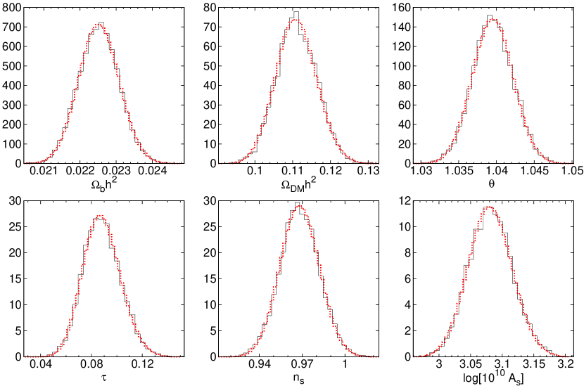
Figure 4.— Marginal cosmological parameter distributions derived with Snake (dashed red line) and CosmoMC (solid black line) from the 7-year WMAP likelihood.

We now apply this method to the 7-year WMAP likelihood, and estimate cosmological parameters within the well-established 6-parameter $\Lambda$CDM concordance model (Komatsu et el., 2011). The parameter set of choice is $\Omega_{b}h^{2}$, $\Omega_{DM}h^{2}$, $\theta$, $\tau$, $n_{s}$ and $\textrm{log}[10^{10}A_{s}]$. The same setup is analyzed using both Snake and CosmoMC for comparison purposes.

The resulting normalized marginal distributions are shown in Figure 4, and means and standard deviations are tabulated in Table 2. The agreement between the two methods is excellent, with a maximum difference between the two methods corresponding to a $0.08\sigma$ shift in $\tau$ and $0.07\sigma$ shift in $n_{s}$.

The CosmoMC results were obtained with an MPI convergence criterion of 0.03, while the Snake convergence threshold was defined to be -6.0. Both codes were run on 50 CPUs, and the resulting wall times were 1.42 and 1.24 hours, respectively.

4.2. Model selection by Bayesian evidence

A significant advantage of Snake over CosmoMC is its direct access to the Bayesian evidence (e.g., Gelman et al., 2003). For a given model $H$ with parameters $\theta$ and data $d$, this is simply the normalization factor, $E\equiv P(d|H)$, in Bayes’ theorem,

$$\textrm{P}(\theta|d,H)=\frac{\textrm{P}(d|\theta,H)\textrm{P}(\theta|H)}{\textrm{P}(d|H)}.$$ (3)

The other factors are the likelihood, $\mathcal{L}(\theta|H)=\textrm{P}(d|\theta,H)$, the prior, $\textrm{P}(\theta|H)$, and the posterior, $P(\theta|d,H)$. Different models can be compared in terms of their evidence, which for a model, $H_{n}$, is given by

$$\textrm{P}(d|H_{n})=\int\limits_{\Omega}\textrm{P}(d,\theta|H_{n})\textrm{d}\theta=\int\limits_{\Omega}\textrm{P}(d|\theta,H_{n})\textrm{P}(\theta|H_{n})\textrm{d}\theta,$$ (4)

where $\textrm{P}(d,\theta|H_{n})$ is the joint probability distribution of $d$ and $\theta$ given this model over all of parameter space, $\Omega$ with step sizes of $\textrm{d}\theta$.

Calculating the evidence for different models using results from Snake is rather straightforward as the parameter space is gridded into even cells of volume ${\int}d\theta$. The integral in equation 4 becomes a sum of the likelihood values within the threshold multiplied by the volume of one grid cell, where we assume a uniform prior which gives a factor of $1/L$ for each parameter, where $L$ is the range for each parameter.

To compare two different models, $H_{1}$ and $H_{2}$, it is common to consider the quantity

$$\delta\textrm{log}E=\textrm{log}E_{1}-\textrm{log}E_{2}$$ (5)

where $E_{1}$ and $E_{2}$ are the evidences of models $H_{1}$ and $H_{2}$, respectively. The larger the value of $\delta\textrm{log}E$ the higher the evidence in favour of model $E_{1}$. To calibrate this quantity, one commonly adopts the Jeffreys’ scale (Liddle et al., 2006; Trotta, 2008), { 1    evidence for $E_{1}$ is substantial $\delta\textrm{log}E>$ 2.5    evidence for $E_{1}$ is strong 5    evidence for $E_{1}$ is decisive.
However, one should note that this scale only provides a general guideline, and conclusions can be application specific; see, e.g., Nesseris & Garcia-Bellido (2012) for a recent discussion of this issue.

We now evaluate the evidence for both the standard six parameter model described above and for a reduced model obtained by enforcing $n_{s}=1$. We find that the individual evidences are $E_{1}=-3743.16$ and $E_{2}=-3744.56$, respectively, with an estimated uncertainty in each of 0.1. This corresponds to $\Delta\textrm{log}E$ of $1.40$ in favour of the 6-parameter model; the full model therefore provides a better fit to the data, even when accounting for the larger parameter volume. Similar results have already been published by Parkinson & Libble (2012). Note that given the full multi-dimensional Snake likelihood, evaluation the evidence of all nested models is trivial by similar calculations.

5. Summary and outlook

In this paper we have described a simple grid-based estimator for multi-dimensional likelihoods. This algorithm exploits the fact that by far most of the $N_{\textrm{par}}$-dimensional parameter volume in a general likelihood has negligible contributions, and spends its computational resources only where the likelihood itself is significant. However, in contrast to standard MCMC methods, it only considers each parameter point once, relying on the actual value of the likelihood.

The main advantages of this method are 1) trivial extraction of arbitrary conditional distributions; 2) direct access to Bayesian evidences; 3) better sampling of the tails of the distribution; and 4) nearly perfect parallelization scaling. The main disadvantage is a computational cost increasing exponentially with $N_{\textrm{par}}$. However, we have shown that the algorithm is fully capable of probing at least $N_{\textrm{par}}\lesssim 12-15$ with reasonable computational resources, which is sufficient for current cosmological models.

In the current implementation the total cost of the method is comparable to that of CosmoMC for similar convergence criteria. However, the cost for a full Snake analysis can be vastly reduced by introducing adaptive grids, in which the grid cell depends on the local properties of the likelihood, such that high-significance regions are sampled more densely than the tail regions. The results from this extension will be reported in a future publication.

References

- Agarwal et al. (2012) Agarwal, S., Abdalla, F. B., Feldman, H. A., Lahav, O., & Thomas, S. A. 2012, MNRAS, 424, 1409
- Auld et al. (2007) Auld, T., Bridges, M., Hobson, M. P., & Gull, S. F. 2007, MNRAS, 376, L11
- Daniel et al. (2012) Daniel, S. F., Connolly, A. J & Schneider, J. 2012, ArXiv e-prints, 1205.2708
- Fendt & Wandelt (2007) Fendt, W. A., & Wandelt, B. D. 2007, ApJ, 654, 2
- Feroz et al. (2009) Feroz, F., Hobson, M. P. & Bridges, M. 2009, MNRAS, 398, 1601
- Frommert et al. (2010) Frommert, M., Pflüger, D., Riller, T., et al. 2010, MNRAS, 406, 1177
- Gelman et al. (2003) Gelman, A., Carlin, J. B., Stern, H. S. & Rubin, D. B. 2003, Dayesian Data Analysis (2nd ed.; Champan & Hall/CRC)
- Jarosik et al. (2011) Jarosik, N. et al. 2011, ApJS, 192, 14
- Komatsu et el. (2011) Komatsu, E., Smith, K. M., Dunkley, J., et al. 2011, ApJS, 192, 18
- Lewis & Bridle (2002) Lewis, A., & Bridle, S. 2002, Phys. Rev. D, 66, 103511
- Liddle et al. (2006) Liddle, A., Mukherjee, P. & Parkinson, D. 2006, Astronomy and Geophysics, 47, 4, 040000-4
- Nesseris & Garcia-Bellido (2012) Nesseris, S., & Garcia-Bellido, J. 2012, arXiv:1210.7652
- Parkinson & Libble (2012) Parkinson, D. & Liddle, A. R. 2010, Phys. Rev. D, 82, 10, 103533
- Planck (2011) Planck Collaboration 2011, A&A, 536, 1
- Sandvik et al. (2004) Sandvik, H. B., Tegmark, M., Wang, X., & Zaldarriaga, M. 2004, Phys. Rev. D, 69, 063005
- Trotta (2008) Trotta, R. 2008, Contemporary Physics, 49, 71-104
- York et al. (2000) York, D. G., Adelman, J., Anderson, Jr., J. E., et al. 2000, AJ, 120, 1579