Angular momentum transfer to a Milky Way disk at high redshift

Abstract

An Adaptive Mesh Refinement cosmological resimulation is analyzed in order to test whether filamentary flows of cold gas are responsible for the build-up of angular momentum within a Milky Way like disk at $z\geq 3$. A set of algorithms is presented that takes advantage of the high spatial resolution of the simulation ($12\,\mathrm{pc}$) to identify: (i) the central gas disk and its plane of orientation; (ii) the complex individual filament trajectories that connect to the disk, and; (iii) the infalling satellites. The results show that two filaments at $z\gtrsim 5.5$, which later merge to form a single filament at $z\lesssim 4$, drive the angular momentum and mass budget of the disk throughout its evolution, whereas luminous satellite mergers make negligible fractional contributions. Combined with the ubiquitous presence of such filaments in all large-scale cosmological simulations that include hydrodynamics, these findings provide strong quantitative evidence that the growth of thin disks in haloes with masses below $10^{12}$ M_☉, which host the vast majority of galaxies, is supported via inflowing streams of cold gas at intermediate and high redshifts.

1 Introduction

Our understanding of the origin of angular momentum within galaxies dates back to the pioneering works of Hoyle (1951) and Peebles (1969), who modelled protogalaxies as spherical Eulerian patches and argued that torques are exerted on a given patch due to tidal interactions with neighbouring patches. Doroshkevich (1970) removed the assumption of spherical symmetry and demonstrated that as perturbations follow the expansion of the background, their total angular momentum evolves with the scale factor as $J(a)\propto a^{3/2}$ in an Einstein–de Sitter universe. An $N$-body simulation study by White (1984) later confirmed that this growth of angular momentum continues until the perturbation, modelled in a Lagrangian framework, breaks away from the background expansion and collapses to form a halo, whereupon its angular momentum remains constant. White (1984) hence argued that the magnitude of the angular momentum acquired for a given halo is set at the epoch of maximum expansion.

A decade after the seminal papers by Peebles (1969) and Doroshkevich (1970), Fall & Efstathiou (1980) expanded beyond the early predictions of tidal torque theory to account for the hierarchical growth of dark matter haloes described in White & Rees (1978), and consequently painted a simple picture of galaxy disk formation. These authors claimed that gas residing in the potential wells of collapsed density perturbations is shock heated to the virial temperature of the halo, and that the inner gas regions subsequently cool and lose their pressure, sinking to the halo centre on a free-fall timescale. Galaxy disks hence form from the ‘inside-out’, as the infalling gas retains its specific angular momentum. Several authors have since reported that the mean stellar age decreases (de Jong, 1996; MacArthur et al., 2004; Gogarten et al., 2010) and specific star formation rates increase (Muñoz-Mateos et al., 2007) as a function of radial position from the disk centre, thereby lending support to the inside-out paradigm of disk growth.

This standard model of disk galaxy formation makes two important assumptions: (i) the specific angular momentum distributions of the gas and virialised dark matter halo are initially equal, and; (ii) the specific angular momentum of the gas is conserved upon collapse to the central disk. This simple model has two appealing features. Firstly, by making a prediction for the relationship between the disk scale length and the host halo virial radius, it is able to recover locally observed distributions of disk scale lengths and the $I$-band Tully–Fisher relation (e.g. Dalcanton et al., 1997; Mo et al., 1998; de Jong & Lacey, 2000). The second success for this model lies in the discovery, using numerical simulations, of the remarkable property that the cumulative fraction of mass within a halo that has specific angular momentum less than $j$, denoted by $M(<j)$, is well fit by a universal function that depends on a single free parameter (Bullock et al., 2001). This result holds for both dark matter and (non-radiative) gas present in haloes of all masses, although the angular momentum vectors of these two components are not generally aligned (van den Bosch et al., 2002).

Despite these successes, recent years have witnessed a resurgence in tackling one of the defining characteristics of the standard theory of disk formation: that gas crossing a halo’s virial sphere is shock heated to the virial temperature of the halo, which typically corresponds to X-ray temperatures of a few $10^{6}\,$K. Binney (1977) was the first to claim that, contrary to the standard paradigm, high density gas in low mass haloes (i.e. most haloes at high redshift) probably crosses an isothermal shock front close to the disk rather than an adiabatic one at the host halo virial radius, and hence argued that the vast majority of gas is expected to stream in towards the disk in cold flows with temperatures close to $10^{4}\,$K. Birnboim & Dekel (2003) reignited this idea by demonstrating that for haloes less massive than $\mathord{\sim}10^{11.6}\,\mathrm{M_{\sun}}$, gas cools efficiently, loses some of its pressure, and is unable to support a virial shock. It was hence concluded that for haloes of mass $M_{\mathrm{H}}\lesssim 10^{11.6}\,\mathrm{M_{\sun}}$, gas flows to the disk in a cold mode as opposed to a hot mode. The lack of redshift evolution in this threshold mass and the penetration of cold streams deep inside the virial region of most haloes was later confirmed by several numerical studies (Kereš et al., 2005; Ocvirk et al., 2008). The existence of a bimodal gas accretion phase potentially has enormous implications for star formation, and may, as the above authors have speculated, account for the observed lack of soft X-ray flux and copious Lyman-$\mathrm{\alpha}$ emission in high redshift galaxies (Birnboim & Dekel, 2003), the bimodality in galaxy colours and its relation to galaxy morphology, including the existence of red galaxies at $z>1$ and massive bursts of star formation at $z\sim 2\mbox{--}4$ (Dekel & Birnboim, 2006), and possibly star formation rate downsizing (Kereš et al., 2005; Ocvirk et al., 2008). These are hence very exciting times for galaxy disk theory.

Having established that gas inflow in most haloes at high redshift proceeds via cold flows that often terminate in the outskirts of gaseous disks (Brooks et al., 2009; Powell et al., 2011), one naturally wonders about the processes governing the transport of angular momentum onto disks within these overdense regions. This is undoubtedly a complex, multiscale problem. On the largest scales of several Gpc, the Universe is thought to be arranged in a complex web of cosmic structure (Bond et al., 1996; Pogosyan et al., 1998), and simulations with differing spatial resolution have helped to decompose the intricate patterns of this web (e.g. Sousbie 2011). It appears that large sheets surrounding Gpc-scale voids intersect to form filaments that funnel gas from the voids to the intersection nodes of the web, where haloes of dark matter form. The amount of mass shared between these separate phases has recently been the subject of debate and involves examining the tidal field tensor that describes the second order derivatives of the gravitational field, in both the linear (Doroshkevich, 1970) and non-linear (Shen et al., 2006; Hahn et al., 2007; Aragón-Calvo et al., 2010) regimes of perturbation growth. Yet the general conclusions of these studies are in agreement: filaments dominate the mass budget. It is hence likely that this component also carries large amounts of angular momentum to the halo nodes of the cosmic web.

Several recent studies have shed some light on the subject of angular momentum transport by filaments on galactic scales. Danovich et al. (2012) performed a statistical study of $350$ Milky Way size dark matter haloes selected from the HORIZON-MARENOSTRUM simulation (details given in Ocvirk et al. 2008, Dekel et al. 2009 and Devriendt et al. 2010) at $z=2.5$ with mass $M_{\mathrm{H}}\simeq 10^{12}\,\mathrm{M_{\sun}}$, whose luminous components were simulated with a physical resolution of $1\,$kpc. They found that the streams of cold gas flowing towards the disk were oriented in a narrow plane, and that the angular momentum transported by this infalling component was highly misaligned with respect to the angular momentum direction of the disk, until the approximate disk boundary, whereupon it dramatically swung into close alignment. An earlier study by Pichon et al. (2011) analyzed several outputs from the same run and examined the nature of filament trajectories on kpc scales, in an attempt to understand the existence of thin gas disks at high redshift that are thought to have formed from the inside-out. These authors demonstrated that material accreted at the virial sphere carried more angular momentum at later times, and attributed this phenomenon to a ‘lever’ mechanism: recently accreted gas has a larger impact parameter owing to the velocity sway of filaments on large scales. It was further hypothesized that these large-scale drift velocities arise from the asymmetric cancellation of motions of gas pumped out of voids. Pichon et al. (2011) hence concluded that the angular momentum transported along cold gas flows into halo virial regions originates from the asymmetry of surrounding large-scale voids. Kimm et al. (2011) investigated these claims by probing an individual halo to a higher physical resolution of $\mathord{\sim}50\,$pc, and found that within the virial sphere, the specific angular momentum of the radiative gas was systematically larger than that of the dark matter. These authors argued that this was a manifestation of a dark matter angular momentum diffusion caused by the mixing of dark matter particles carrying different amounts of angular momentum at the time of accretion (this mixing is due to the dark matter undergoing shell-crossing as it passes through walls and filaments, before entering the host’s virial region). They justified this claim by demonstrating that there was a large distribution in the age of the dark matter particles at any given radius (see also the impact parameter distributions and backslash velocities measured at the virial radius in Figs. 15 and 20 of Aubert & Pichon 2007). On the other hand, the halo gas does not experience the same angular momentum diffusion since it streams almost exclusively along filaments (i.e. in a preferential direction) towards the central region where it eventually experiences an isothermal shock and remains trapped (Birnboim & Dekel, 2003; Kereš et al., 2005; Ocvirk et al., 2008). Kimm et al. (2011) demonstrated that this does indeed happen by showing that the amount of specific angular momentum transported by gas was constant with radius at both low ($0\leq z\leq 3$) and high ($z>3$) redshifts, except for $r\lesssim 0.1r_{\mathrm{vir}}$, whereupon it fell dramatically. This hints at unresolved complex dynamics within the ‘disk’ region (e.g. Book et al. 2011) of high redshift galaxies.

Yet due to physical resolution constraints, the Kimm et al. (2011), Pichon et al. (2011) and Danovich et al. (2012) studies were neither able to accurately resolve the disk scaleheight and scalelength at high redshift, nor the dynamics within the disk region. By analyzing outputs from one of the high resolution NUT simulations (see Powell et al., 2011), which tracks the high redshift evolution of a single Milky Way like galaxy with a physical resolution scale of $12\,$pc, this paper rises to the challenge of attempting to account for the amount of angular momentum locked-up in a Milky Way like disk that resides in a halo fed by streams of cold gas, and complements the papers listed above. The aim is to ascertain whether filaments dominate the angular momentum budget of the central disk across time. This would provide quantitative evidence in favour of the cold mode of disk growth, a theory currently lacking observational confirmation (Faucher-Giguère et al., 2010; Steidel et al., 2010, but see Fumagalli et al. 2011).

This paper is arranged as follows. In Section 2, the details of the simulation and the physics encoded within it are briefly discussed. The various algorithms that have been developed to: a) compute the orientation plane of the resimulated Milky Way like disk; b) resolve the individual gas filaments and satellites that merge onto it, and; c) quantify the angular momentum locked-up in each of these galaxy components, are then introduced in Sections 3 and 4. A more detailed description of the filament and satellite identification algorithms is provided in Appendices A and B respectively. Section 5 presents the results, Section 6 discusses their implications, and Section 7 summarizes our conclusions.

2 The simulation

2.1 The NUT cooling run

We examine one of the NUT simulations to understand how a Milky Way like disk acquires its angular momentum. The NUT suite (Powell et al., 2011) is a set of ultra-high resolution simulations that employ a zoom technique (see e.g. Navarro et al., 1995) to resimulate a Milky Way like galaxy and follow its evolution across redshift in a $\Lambda$CDM cosmology. The resolution and number of physical processes that are modelled vary from one simulation to the next. The highest resolution runs in the NUT suite have a maximum spatial resolution $\Delta x_{\mathrm{res}}$ of $0.5\,$pc but terminate at high redshifts ($z\simeq 6$) due to computational time restrictions, and so in this paper a lower resolution $\Delta x_{\mathrm{res}}=12\,$pc run is analyzed as it probes redshifts down to $z=3$. More specifically, the NUT cooling run, hereafter NutCO run, examined in this paper has been performed using the publicly available Adaptive Mesh Refinement (AMR) code RAMSES (Teyssier, 2002), incorporating the following physics:

1. Epoch of reionization—a spatially uniform, redshift-dependent ultraviolet (UV) background instantaneously switched on at $z=8.5$ (following the Haardt & Madau 1996 UV model).

2. Cooling and star formation.

The important technical details of the NutCO run are now briefly summarized. The chosen resimulated Milky Way like halo satisfies two conditions: it is a typical 2$\sigma$ density fluctuation, i.e. it is not embedded in a denser group or cluster environment at $z=0$, and its present day mass ($M_{\mathrm{H}}\simeq 5\times 10^{11}\,\mathrm{M_{\sun}}$) is comparable to the threshold mass ($M_{\mathrm{H}}\sim 4\times 10^{11}\,\mathrm{M_{\sun}}$) reported by Ocvirk et al. (2008) below which gas streams along filamentary structures at low temperatures of T $\lesssim 2\times 10^{4}\,$K. The entire simulation box has a comoving side length of $9\,h^{-1}\,$Mpc and starts at $z=499$, with the initial conditions generated using the package MPgrafic (Prunet et al., 2008). The resimulation box around the main halo has a comoving side length of $\mathord{\sim}2.7\,h^{-1}\,$Mpc, and the simulation evolves in a universe of WMAP5 cosmology (Dunkley et al., 2009) with $\Omega_{\mathrm{M}}=0.258,\Omega_{\Lambda}=0.742$, $\Omega_{b}=0.045,\sigma_{8}=0.8$ and $h=0.72$. The coarse root grid for the entire simulation has $128$ cells along each dimension of the $9\,h^{-1}\,$Mpc box, whereas the resimulated region contains three higher resolution nested grids yielding an equivalent particle resolution of $1024^{3}$ dark matter particles, each with mass $M_{\mathrm{DM}}=5.4\times 10^{4}\,\mathrm{M_{\sun}}$. A quasi-Lagrangian refinement scheme is used to maintain $\Delta x_{\mathrm{res}}=12\,$pc in physical coordinates as the simulation evolves. Higher levels of refinement are spawned once either: a) the baryonic mass in the cell exceeds $8m_{\mathrm{SPH}}$ ($m_{\mathrm{SPH}}=9.4\times 10^{3}\,\mathrm{M_{\sun}}$) or; b) the number of dark matter particles in the cell exceeds eight. This scheme therefore strives to achieve a roughly equal gas mass per cell.

The NUT simulation includes stars and so a brief discussion of the prescriptions used for modelling star formation, which are described in detail by Rasera & Teyssier (2006), is now provided. The gas in a cell can cool to temperatures $T\sim 10^{4}\,$K via bremsstrahlung radiation (effective until $T\sim 10^{6}\,$K), and via collisional and ionization excitation followed by recombination (dominant for $10^{4}\leq T/\mathrm{K}\leq 10^{6}$). The metallicity of the gas is fixed to $10^{-3}\,\mathrm{Z_{\sun}}$ to allow further cooling to molecular cloud temperatures of $\mathord{\sim}1\,$K via metal line emission, and once the gas is sufficiently dense (i.e. $\rho>\rho_{0}$, where $\rho_{0}$ is a density threshold and is chosen to represent the density of the interstellar medium, hereafter ISM), star formation naturally ensues, a process which is modelled by a Schmidt law (Schmidt, 1959). The star formation efficiency parameter $\epsilon$ is fixed at $1\%$ per free-fall time in concordance with observations (Krumholz & Tan, 2007) and $\rho_{0}$ is chosen to be equal to $400$ hydrogen atoms per cubic centimetre. If the Jean’s scale $\lambda_{\mathrm{J}}$ is close to or below the minimum resolved scale $\Delta x_{\mathrm{min}}$ (determined by the highest level of refinement $\ell_{\mathrm{max}}$), it is possible that gas clouds artificially fragment, leading to artificial star formation. Therefore, when in excess of the ISM density $\rho_{0}$, the gas is forced to follow a polytropic equation of state. The number $N$ of stellar particles that form in a cell whose gas is sufficiently cool and dense is drawn from a Poisson distribution, based on the cell mass, the local star formation timescale, and the minimum stellar mass allowed for a star particle $m_{\star,\mathrm{min}}$, which itself is proportional to the minimum cell volume. In order to prevent an overproduction of stellar particles in a given cell, all of the $N$ newly formed stellar particles are then merged into a single particle of mass $m_{\star}=Nm_{\star,\mathrm{min}}$. Stellar particles in the NutCO run analyzed in this study are therefore stellar clumps of up to several thousand stars.

2.2 Identifying (sub)haloes & galaxies and following their merger histories

The Most massive Sub-node Method subhalo-finding algorithm, hereafter MSM (Tweed et al., 2009), was used in order to detect the haloes, subhaloes, stellar clumps and stellar subclumps at each time output of the NutCO run. MSM assigns a local density estimate to each particle computed using the standard Smoothed Particle Hydrodynamics kernel (Monaghan & Lattanzio, 1985), which weights the mass contributions from the $N$ closest neighbouring particles ($N=20,32$ for the haloes and stellar clumps, respectively). Haloes are then resolved by imposing a density threshold criterion and by measuring local density gradients. In order to detect host haloes, stellar clumps and associated levels of substructure, MSM successively raises the density thresholds on the host until all of its node structure has been resolved. The most massive leaf is then collapsed along the node tree structure to resolve the main halo or the main stellar clump and the same process is repeated for the lower mass leaves, defining the embedded substructures.

Each resolved halo (stellar clump) object is forced to contain at least $40$ ($100$) particles to ensure reliable detections. Note that the stellar clump resolution limit is set above the dark halo limit to avoid identifying groups of stars within the disk as independent objects. The TreeMaker code (Tweed et al., 2009) is then used to link together all the time outputs by finding the fathers and sons of every halo and subhalo, and every stellar clump and subclump.

3 Resolving the galaxy components

This section describes the algorithms that have been used to identify the likely sources of the disk’s angular momentum within the host’s virial region. The following terms—$r_{\mathrm{vir}}$, disk, satellites and virial sphere—are henceforth made in reference to the NUT host halo.

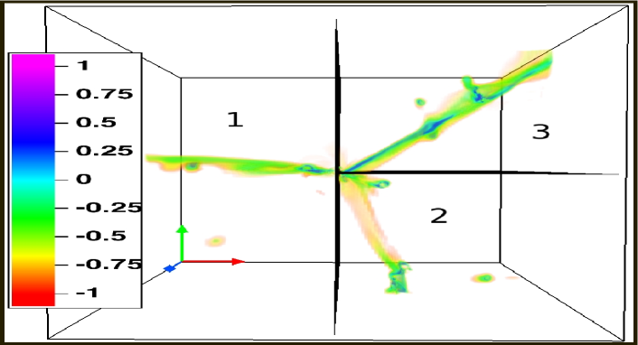
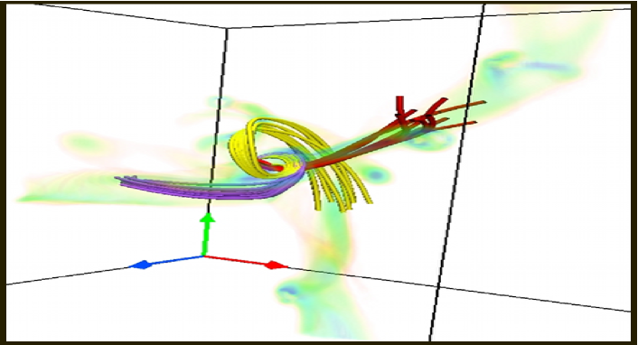
Figure 1: Images of the filament gas within a box centred on the main host at $z\sim 10$ (left) and $z\sim 8$ (right) in the NutCO run, generated using the Visualization and Analysis Platform for Ocean, Atmosphere, and Solar Researchers software (commonly referred to as VAPOR, see https://www.vapor.ucar.edu/ for details). The sidelength of the box in the left panel corresponds to $4r_{\mathrm{vir}}$ ($\mathord{\sim}17\,$kpc) and this face-on view illustrates the clear separation of the filaments into three distinct regions (labelled accordingly) at large scales and early times. The image in the right panel shows the inner virial region ($\mathord{\sim}7.5\,$kpc) at lower redshift when the dynamics of the system have changed, and the velocity flow tubes demonstrate the complex trajectories of gas flow within the gas disk region, colour coded according to the filament that they are likely to trace. The density of the gas has been dimmed and the viewing angle rotated to best highlight each trajectory. Both panels have been refined to $\ell=16$, corresponding to a physical cell width of $\mathord{\sim}17\,$pc (left) and $\mathord{\sim}22\,$pc (right), and the colour bar indicates the gas density in dimensionless units of $\mathrm{log_{10}(n/cm^{-3})}$, where $n$ is the number density of hydrogen atoms per cubic centimetre. Filament gas has been detected by applying the $nT$ criteria, but gas with density $\mathrm{log_{10}(n/cm^{-3})}<-1$ has been excluded from both figures for clarity. The rightward red, upward green and forward blue axes correspond to the $x$, $y$ and $z$ directions, and the vertical and horizontal black planes in the left panel show the spatial cuts in the $x$ and $y$ directions that have been used to start the colouring of the tracer particles, which is a technique that has been developed to separate each of the filaments at high redshift (see Section 3.2 and Appendix A).

3.1 Grid notations

This study analyzes cubic and spherical grids $\mathcal{G}_{x}$ centred on the galaxy (i.e. on its most dense cell) with physical half-lengths and radii equal to $xr_{\mathrm{vir}}$, where $x\in\{0.1,0.15,0.5,1.0,2.0\}$. The numerical subscript $x$ will be explicitly stated when discussing a certain grid type, but for comparisons between grid types (e.g. the gas grid $\mathcal{G}_{g}$ or the stellar grid $\mathcal{G}_{\star}$) it is replaced by a symbol denoting the type, and the extent of the grid is implicitly understood. All of the spherical (cubic) grids in this paper with physical diameter (full-length) $L$ are subdivided into $n$ cubic cells of equal physical sidelength $\Delta x$ and are hence ‘fixed’, obeying the relation:

$$\Delta x=\frac{L}{n}.$$ (1)

Since there are $2^{\ell}$ cells along each dimension of the physical simulation grid length $L_{s}(z)$ at level $\ell$, it follows that the refinement level of $\mathcal{G}_{x}$ is given by:

$$\ell=\frac{\ln\left(L_{s}/\Delta x\right)}{\ln\,2},$$ (2)

where $L_{s}(z)=9\,h^{-1}\,\mathrm{Mpc}/(1+z)$ and $\ell$ is rounded to its nearest integer value. The routines that generate fixed density, temperature and velocity grids at a given location by performing an interpolation from the simulation grid for gas properties and a Cloud-in-Cell smoothing technique for particle properties, require $L$ and $\ell$ as inputs at runtime. Memory and CPU time constraints mean that $n$ is not allowed to exceed $1024$, however, so we decrease $\ell$ successively in integer units in equation (2) until this constraint is satisfied. As a result, the resolution $\Delta x$ for the grids enclosing the $r_{\mathrm{vir}}$ and $2r_{\mathrm{vir}}$ regions deviates from the maximum resolution $\Delta x_{\mathrm{res}}$ for low redshift outputs, as the virial radius of the host (and hence $L$) expands. However, this ‘time bias’ does not affect the grids $\mathcal{G}_{0.1}$ and $\mathcal{G}_{0.15}$ used for performing the angular momentum computations (see Section 4), as their cell width remains equal to $\Delta x_{\mathrm{res}}$ at all times.

3.2 Disentangling the filaments using a tracer particle colouring algorithm

Powell et al. (2011) have shown that parcels of gas whose number density of hydrogen atoms $n$ and temperature $T$ simultaneously satisfy $0.1\leq n/\mathrm{cm}^{-3}\leq 10$ and $T/\mathrm{K}\leq 2\times 10^{4}$, are representative of gas belonging to filaments in the NUT simulations at high redshift ($z\geq 9$). The analysis in this work resolves the NUT filaments down to $z=3$, hence in order to tackle the possible time evolution in their density, this paper uses the prescription between the lower threshold and the background density introduced by Kimm et al. (2011), who argued that large-scale filament density is gravitationally coupled to the expansion of the Universe. They defined the lower number density bound $n_{\mathrm{L}}$ as:

$$n_{\mathrm{L}}\equiv\frac{\delta_{f}\bar{\rho}f_{b}X_{\mathrm{H}}}{m_{\mathrm{H}}},$$ (3)

where $\bar{\rho},\delta_{f},f_{b},X_{\mathrm{H}}$ and $m_{\mathrm{H}}$ are respectively the mean density of the background, the density contrast of the filament (measured with respect to $\bar{\rho}$), the fraction of the total mass in baryons ($\equiv\Omega_{b}/\Omega_{\mathrm{M}}$), the primordial relative mass abundance of hydrogen ($76\%$), and the mass of a hydrogen atom. A typical value of $n_{\mathrm{L}}$ from the NutCO run at $z=3$ is $\mathord{\sim}0.01\,\mathrm{cm^{-3}}$.

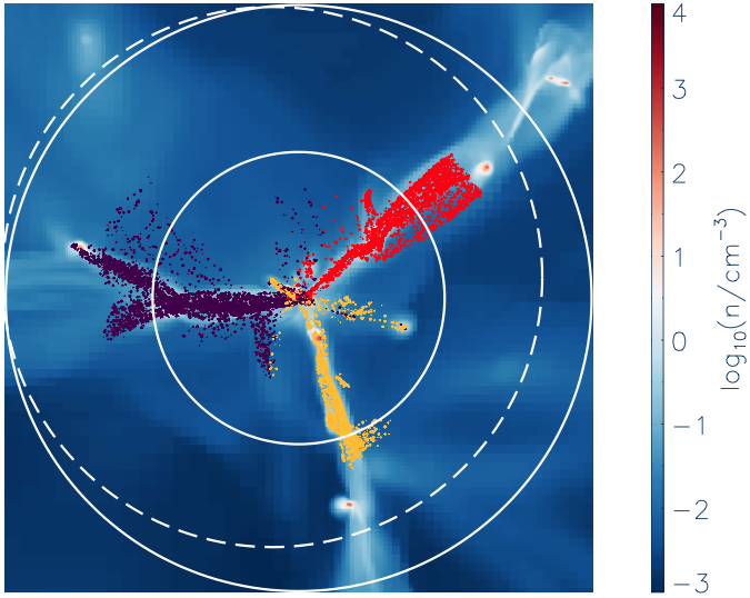
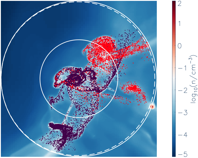
Figure 2: These gas density images are $z$ projections of the large-scale region surrounding the central disk in the NutCO run, and illustrate the spatial distribution of particles tracing the filaments at $z\sim 9$ (left panel) and $z=3$ (right panel). The inner and outer solid circles have radii equal to $r_{\mathrm{vir}}$ and $2r_{\mathrm{vir}}$ respectively, where $r_{\mathrm{vir}}\sim 5.3\,$kpc (left) and $r_{\mathrm{vir}}\sim 31\,$kpc (right). The dashed circles represent the $2r_{\mathrm{vir}}$ regions at the previous time output, corresponding to $z\sim 9.5$ ($r_{\mathrm{vir}}\sim 4.7\,$kpc) and $z\sim 3.04$ ($r_{\mathrm{vir}}\sim 30\,$kpc). All of the circles are centred at the location of the densest cell in the disk region at the relevant time output. Left panel: Those tracer particles that have been identified with each of the purple, yellow and red filaments at $z\sim 9.5$ and that coincide with filament cells refined to $\ell=15$ ($\Delta x\sim 38\,$pc) at $z\sim 9$, have been updated to their new positions. The offset in centres between the outer solid and dashed circles arises due to the motion of the centre of disk rotation, and the gap between each set of coloured tracers and the dashed circle highlights the displacement of the tracers over the time interval. Uncoloured new tracer particles that have crossed the $2r_{\mathrm{vir}}$ sphere over the interval and that move along filament trajectories at $z\sim 9$ have been omitted. Right panel: The filament configuration at $\ell=14$ ($\Delta x\sim 190\,$pc) for the final time output at $z=3$. This image includes both updated coloured tracers and new tracers that have been assigned a colour using the nearest neighbours method (see text). In Section 5 it is demonstrated that the purple and yellow filaments start to merge around $z\sim 5.5$, with the former filament surviving, and this is confirmed by the absence of yellow tracers in this panel. Only $5\%$ of all the coloured filament tracers are shown at this time output, for clarity.

It was also found that an upper temperature limit of $T_{u}\leq 2\times 10^{5}\,$K (e.g. Kereš et al. 2009; Faucher-Giguère et al. 2011) detected filaments to a higher level of accuracy for $z\geq 3$ in the NutCO run than the classical cold mode temperature of $T_{u}\leq 2\times 10^{4}\,$K (e.g. Kay et al. 2000; Birnboim & Dekel 2003; Kereš et al. 2005) at which gas is thought to cool via Lyman-$\alpha$ emission (e.g. Fardal et al. 2001). There are two reasons for this. Firstly, once reionization has completed ($z_{\mathrm{re}}=8.5$), the UV background heats all the gas uniformly, without taking into account its capacity to self-shield from UV photons in denser environments. Secondly, the absence of metal production sources in the NutCO run causes the gas metallicity to remain fixed at its very low initial value (10^-3 Z_☉). As a consequence, cooling is inefficient and filaments stay hotter for longer (e.g. Sutherland & Dopita 1993).

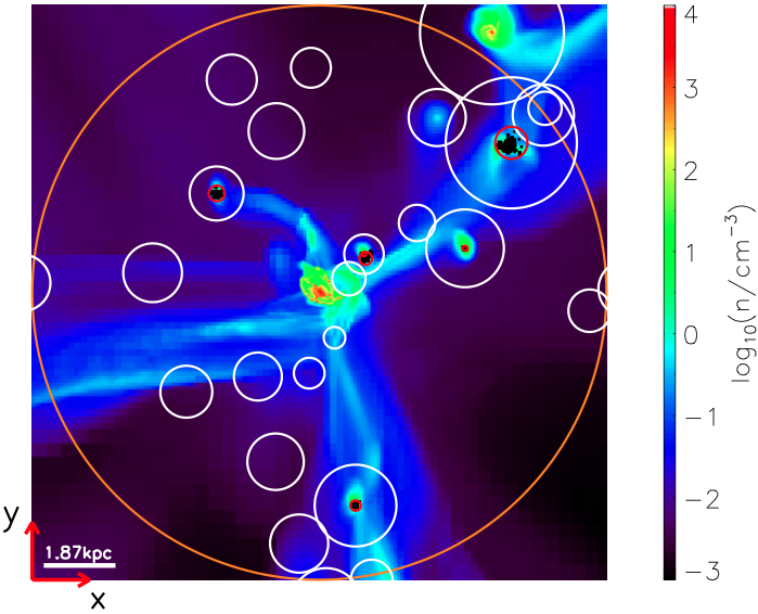
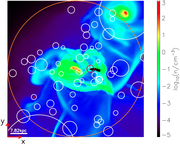
Figure 3: Projections along the $z$ direction of all the gas within a box of sidelength equal to $2r_{\mathrm{vir}}$, corresponding to the diameter of the orange circles. The centre of each image coincides with the centre of the stellar clump of the host galaxy at $z\sim 8$ (left) and $z=3$ (right), with $\ell=16$ ($\Delta x\sim 22\,$pc) and $\ell=15$ ($\Delta x\sim 95\,$pc). The virial regions of the stellar and dark halo satellites of the main host, as identified by the satellite-finding algorithm, are shown by the red and white circles respectively, with each circle centred at the densest member star identified as part of the satellite. The constituent satellite stars have been detected by the clump-finder, and are shown as small filled black circles. The white horizontal bars and vertical colour bars indicate the length scale (in physical kpc) and the density colour scale (in dimensionless units of $\mathrm{log_{10}}$ number of hydrogen atoms per cubic centimetre) respectively. Note that the large stellar satellites in the upper right corners of both panels have not been identified as luminous satellites because their stellar virial regions do not infringe the host’s virial sphere at these epochs.

Hence, in order to identify the neutral hydrogen and helium gas in the filamentary phase in the NutCO run, the density and temperature criteria, hereafter $nT$, reported by Powell et al. (2011) have been used for $z\geq 3$, but the lower density threshold has been replaced by the value given by equation (3) and the upper temperature limit has been increased to $T_{u}=2\times 10^{5}\,$K. The left panel in Fig. 1 shows an image of the three filaments within $2r_{\mathrm{vir}}$ of the host centre at $z\sim 10$ in the NutCO run, found by imposing these $nT$ criteria. The filaments occupy three distinct regions on large scales at this epoch and the flow appears to be ordered and mostly radial (a discussion of how gas that is shared by filaments and satellites is apportioned between these two phases is preserved for Section 3.3). The dynamics of the gaseous motions in the central region are far more complex, however, as demonstrated in the right panel, which shows the velocity flow vectors of filament gas within the virial region at a later time (corresponding to $z\sim 8$) when the system has evolved to a different configuration. The individual filament trajectories bend, twist and mix with each other in the central region, yet often remain intact. In order to test the hypothesis that the disk acquires its angular momentum from filamentary motions, it is critical to follow these separate individual filament trajectories. A suitable tool for performing this Lagrangian exercise is the use of tracer particles (e.g. Dubois et al., 2012), which have been demonstrated to preferentially trace filament flows in galaxy simulations (Pichon et al., 2011). The tracer particles in the NUT suite have an identical spatial distribution to dark matter at the beginning of the simulation, and are assigned zero mass. They are simply advected with the gas and can therefore be used to track its velocity field within the host virial region.

The algorithm that resolves each filament at high redshift is henceforth referred to as the ‘tracer propagation method’, and is described in detail in Appendix A, which also includes a discussion of the (negligible) uncertainties associated with the method. The main idea is to assign the tracer particles within each filament a unique colour at some early time, and then use a nearest neighbours scheme to construct the individual filament trajectories within the host virial region at later times. Throughout this paper reference is made to the purple, yellow and red filaments in regions $1,2$, and $3$ of the left panel of Fig. 1 respectively. The left panel of Fig. 2 shows tracer particles colour coded according to the filament they sample at $z\sim 9.5$, updated to their new filament positions at $z\sim 9$. The displaced tracers extend across the full virial region at $z\sim 9$ (given by the inner solid circle), and so new tracers entering the $2r_{\mathrm{vir}}$ region at this epoch (denoted by the outer solid circle) are appropriately coloured. Since colour is propagated across time, one is able to test the overall performance of the method by considering the final output. Coloured filament tracers within $2r_{\mathrm{vir}}$ at $z=3$ are hence shown in the right panel of Fig. 2 (only $5\%$ of all the coloured filament tracers are plotted for clarity, but this subsample is representative of the whole distribution). The purple and yellow filaments undergo a merger around $z\simeq 5.5$ in the simulation (this is discussed in more detail in Section 5), and the algorithm clearly captures the aftermath of this merger as only the purple and red tracer particles remain at $z=3$. The filaments are highly perturbed within the inner virial region and trace complex trajectories, no longer displaying the ordered gas inflow seen at higher redshift in the left panel.

3.3 Locating the satellites

There are two types of satellites in the simulation: ones with a dark matter halo and ones whose dark halo component has been stripped by tidal forces to the extent that it does not contain enough particles to be detected by the halo finder. One property all satellites share in common, however, is that they are substructures of the main host. As shown in the left panel of Fig. 3, luminous satellites in the simulation are often found to stream along filaments, eventually merging onto the central disk, perhaps transporting large amounts of angular momentum in the process. One is therefore faced with the following dilemma: should the angular momentum of gas gravitationally bound to a satellite, which itself is drifting along a filament, be solely attributed to the satellite? The answer to this question in this study is chosen to be ‘no’: only gaseous material within the virial region of a satellite that does not satisfy the $nT$ criteria in that it lies above the upper filament density cut, is apportioned to the satellite phase. ‘Satellite’ is therefore made in reference to the central dense galaxy component which dominates the ‘true’ satellite angular momentum signal. The advantages of this satellite definition are two-fold:

• only small regions are masked from the density field, leaving the filament trajectories largely unperturbed, and;

• the highest density material that is likely to dominate the satellite angular momentum budget is accounted for.

The satellite identification procedure used in this study locates subhaloes of the main host that were once themselves field haloes earlier in their accretion history. Fig. 3 shows $z$ projections of the gas density within the host virial region (orange circle) at $z\sim 8$ (left panel) and $z=3$ (right panel), and includes all the dark matter satellites (white circles) and stellar satellites (red circles) that have been found by applying the satellite identification technique, which is described in detail in Appendix B. Each of these circles is centred on the centre of the galaxy it represents, as identified by the halo and stellar clump-finder. The filled black circles correspond to the constituent stellar particles of each stellar satellite, which can violate the virial accuracy condition imposed by the MSM halo-finder and can hence lie beyond their host’s virial region, as illustrated for the elongated satellite in the right panel. Clearly the apparent luminous satellites in Fig. 3 are captured by the satellite-finding algorithm at the two extrema of the range in epochs examined in this study.

4 Angular momentum measurement techniques

4.1 Calculating angular momentum in the general case

Unless stated otherwise, the total angular momentum $\mn@boldsymbol{J}$ has been computed by using the following expression:

$$\mn@boldsymbol{J}=\sum_{i}m_{i}{(\mn@boldsymbol{r}_{i}-\mn@boldsymbol{r}_{c})\times(\mn@boldsymbol{v}_{i}-\mn@boldsymbol{v}_{c})},$$ (4)

where $i$ refers to either a stellar particle, a dark matter particle or a gas cell of mass $m_{i}$ at location $\mn@boldsymbol{r}_{i}$ with velocity $\mn@boldsymbol{v}_{i}$, and $\mn@boldsymbol{r}_{c}$ and velocity $\mn@boldsymbol{v}_{c}$ refer to the centre of rotation within the central galaxy. There are two suitable estimators for these latter quantities: 1) the densest cell, which is likely to correspond to the disk centre, and; 2) the centre of mass. Both of these definitions have been found to yield very similar estimates of $\mn@boldsymbol{r}_{c}$ and $\mn@boldsymbol{v}_{c}$ in the NutCO run, but at high redshifts where the main host undergoes major mergers, it sometimes happens that the centre of mass is located in a region relatively devoid of mass, which does not correspond to the centre of the disk. We therefore adopt the densest cell as the best estimate of $\mn@boldsymbol{r}_{c}$, which has been computed by simply summing the gas $\mathcal{G}_{g}$, stellar $\mathcal{G}_{\star}$ and dark matter $\mathcal{G}_{\mathrm{DM}}$ grids within $0.1r_{\mathrm{vir}}$ of the host centre and locating the member cell of their sum $\mathcal{G}_{0.1}$ with the most mass. The velocity of the centre of disk rotation $\mn@boldsymbol{v}_{c}$ has been approximated by the centre of mass velocity $\mn@boldsymbol{v}_{\mathrm{com}}$ of $\mathcal{G}_{0.1}$. Since there are a large ($\gg 10^{6}$) number of cells and particles that contribute to $\mn@boldsymbol{v}_{\mathrm{com}}$ at all times, noise is low and this velocity should thus be very close to the true bulk velocity of the disk.

4.2 Obtaining the equation of the gas disk’s plane of rotation

It is assumed that the rotation of the gas disk is confined to a single plane centred on $\mn@boldsymbol{r}_{c}$ at all times, and an estimate for the equation of this plane has been made by using equation (4) to compute the disk angular momentum $\mn@boldsymbol{J}_{d}$. All of the gas within $\mathcal{G}_{0.1}$ associated with the luminous satellites (identified using the satellite-finding technique) and the filaments (identified using the $nT$ criteria) has been flagged, and the remaining gas in this region is assigned to the disk. Fig. 4 shows a density image of the gas disk at $z=3$ in the NutCO run, and overplots the plane found by adopting the above disk definition. The excellent agreement between the computed disk plane and its apparent orientation in Fig. 4 provides confirmation that the disk definition and estimates of $\mn@boldsymbol{r}_{c}$ and $\mn@boldsymbol{v}_{c}$ in equation (4) are reliable.

4.3 Quantifying angular momentum transport to the disk

The material channelled inward along filaments $f$ in the simulation gets compressed once it settles into the disk $d$, and star formation ensues when the gas is sufficiently dense. Mass and angular momentum transported by these flows is hence assumed to be shared amongst the central baryons $b$, as shown below by the arrows. The central baryons refer to both the gas in the disk and the stars that form from the disk’s fragmentation:

$$m_{f}\to m_{b} = m_{d}+m_{\star}$$ (5)

$$\mn@boldsymbol{J}_{f}\to\mn@boldsymbol{J}_{b} = \mn@boldsymbol{J}_{d}+\mn@boldsymbol{J}_{\star}.$$ (6)

At a given time output, a list of identifiers of every particle that has ever been resolved as a member constituent of a satellite, as detected by the satellite-finding algorithm over the Milky Way host’s virial region, is updated. Hence $\mn@boldsymbol{J}_{\star}$ has been computed at each epoch by using equation (4) and including each particle within $0.1r_{\mathrm{vir}}$ that does not belong to this list. These non-satellite stars correspond to bulge and disk stars, but the former component has a weak angular momentum modulus (see e.g. van den Bosch et al. 2002) and so the stellar disk signal dominates $\mn@boldsymbol{J}_{\star}$. Hence, even though $m_{b}$ and $\mn@boldsymbol{J}_{b}$ refer to the total (stars plus gas) mass and angular momentum of the ‘baryonic galaxy’ in what follows, we will often abbreviate this to ‘the disk’. By excluding contributions from satellite stars, equations (5) and (6) focus on in situ disk formation.

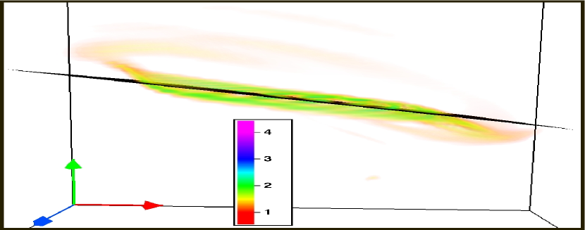
Figure 4: A VAPOR visualization in density of the gas disk refined to $\ell=18$ ($\Delta x\sim 12\,$pc) at $z=3$. The black slice shows the plane of disk rotation found by computing the disk angular momentum $\mn@boldsymbol{J}_{d}$ within $\mathcal{G}_{0.1}$ (equation 4). The scaled sidelength of the box in this image is approximately $6\,$kpc in physical coordinates, and the set of orthogonal axes and the units of the colour bar are the same as in Fig. 1.

We now compare $\mn@boldsymbol{J}_{b}$ at each time output with the accumulated angular momentum brought in by the satellite and cold filament gas within $0.1r_{\mathrm{vir}}$, since these components are thought to fuel the disk’s angular momentum budget. We also estimate the fraction of $\mn@boldsymbol{J}_{b}$ acquired via a hot mode of gas accretion, as this enables direct comparisons with the cold mode signals. This hot gas phase is populated by selecting all of the gas cells with a temperature above the imposed upper temperature limit of the cold phase (i.e. $T>2\times 10^{5}\,$K). Hot gas should not be regarded as a separate component, however, because these cells are included in the satellite and disk signals by construction (see Section 4.2).

4.3.1 The hot and cold phase contributions to $m_{b}$ and $\mn@boldsymbol{J}_{b}$

Estimates of the angular momentum accumulated onto the disk via the accretion of hot and cold gas have been made by time-integrating the instantaneous flow rates of these components across a thin spherical shell located on the periphery of the disk region. This is a suitable method to employ because the inflowing gas in the simulation settles onto the disk very rapidly after crossing the shell (the validity of this assumption is tested in the following section). The flow rates have been computed by using the technique described in Powell et al. (2011), and for simplicity, reference is made to the filament gas phase in the descriptions below (but the same equations apply to the hot mode):

$$\frac{\mathrm{d}\mn@boldsymbol{J}}{\mathrm{d}t} = \frac{\sum_{i}\rho_{i}v_{r,i}\left[(\mn@boldsymbol{r}_{i}-\mn@boldsymbol{r}_{c})\times(\mn@boldsymbol{v}_{i}-\mn@boldsymbol{v}_{c})\right](\Delta x)^{3}}{\sum_{j}(\Delta x)^{3}}4\pi r_{m}^{2}$$ (7)

$$\frac{\mathrm{d}M}{\mathrm{d}t} = \frac{\sum_{i}\rho_{i}v_{r,i}(\Delta x)^{3}}{\sum_{j}(\Delta x)^{3}}4\pi r_{m}^{2}.$$ (8)

The sum indexed by $j$ is performed over all of the cells in the shell, irrespective of their gas phase, and $\mn@boldsymbol{r}_{c}$ and $\mn@boldsymbol{v}_{c}$ are the same as in equation (4). The variables $\mn@boldsymbol{r}_{i},\mn@boldsymbol{v}_{i}$ and $\rho_{i}$ correspond respectively to the position, velocity and density of the $i^{\mathrm{th}}$ cell satisfying the relevant imposed condition, which in this case is the requirement that $i$ is a filament cell. Equations (7) and (8) hence yield the net radial flux transported across the spherical shell towards (negative sign) or away from (positive sign) the disk, where the radial velocity of each cell is given by:

$$v_{r,i}=(\mn@boldsymbol{v}_{i}-\mn@boldsymbol{v}_{c})\cdot\frac{\mn@boldsymbol{r}_{i}-\mn@boldsymbol{r}_{c}}{|\mn@boldsymbol{r}_{i}-\mn@boldsymbol{r}_{c}|}.$$ (9)

It follows that the total angular momentum (and mass) transferred towards the disk by each filament over the time interval $\Delta t=t-t_{i}$ is:

$$\Delta\mn@boldsymbol{J}_{\mathrm{flux}}(t) = \int_{t_{i}}^{t}\frac{\mathrm{d}\mn@boldsymbol{J}}{\mathrm{d}t}\,\mathrm{d}t$$ (10)

$$\simeq \left(\frac{\mathrm{d}\mn@boldsymbol{J}}{\mathrm{d}t}\bigg{|}_{t}+\frac{\mathrm{d}\mn@boldsymbol{J}}{\mathrm{d}t}\bigg{|}_{t_{i}}\right)\frac{\Delta t}{2},$$ (11)

where the latter step approximates the integral by a simple numerical trapezium integration, i.e. a linear interpolation of the unresolved flow rates between time outputs. The signal found using the ‘spherical flux technique’ of equation (11) at $t$ is then accumulated with the corresponding signals at earlier times.

The summations indexed by $i$ in equations (7) and (8) include all of the filament cells whose centres lie within a shell of inner, outer and mid radius $r_{\mathrm{in}}=r_{m}-\Delta r/2$, $r_{\mathrm{out}}=r_{m}+\Delta r/2$ and $r_{m}=0.1r_{\mathrm{vir}}$, respectively. The thickness of the shell $\Delta r$ is a free parameter and has been fixed to $1\%$ of $r_{\mathrm{vir}}$ (i.e. one tenth of the $0.1r_{\mathrm{vir}}$ radius) at each time output, as this choice strikes a good compromise between negligible Poisson error and the validity of the thin shell approximation (the shells typically included $\mathord{\sim}2\times 10^{5}$ cells at the highest redshifts around $z\sim 9$ and $\mathord{\sim}2\times 10^{7}$ cells at the lower redshifts around $z\sim 3$, where the shell is physically larger). Similar flux measurements were found for shell thicknesses between $\mathord{\sim}0.1\mbox{--}2.5\%$ of $r_{\mathrm{vir}}$, which implies that there is some flexibility in the value assigned to $\Delta r$. A larger grid than $\mathcal{G}_{0.1}$ is therefore required, in order to compensate for the half of the shell that spills beyond the $0.1r_{\mathrm{vir}}$ region. The filaments are thus constructed over a $0.15r_{\mathrm{vir}}$ region according to step $3$ of the colour propagation scheme described in Appendix A. This particular grid length is chosen because the physical width of the cells within $\mathcal{G}_{0.15}$ is still at the $12\,$pc limit for every time output, and so the extra grid length makes no difference to the accuracy of the mass and angular momentum computations.

It is clear from the above that a decision has been made to represent the quantities $r_{m}$ and $\Delta r$ as fractions of the host’s virial radius, which grows with time in the simulation. The spherical flux method hence sweeps up gas by construction, and a simple trapezium integration of radial flux signals across the shell could miss this component if the filament’s trajectory is mostly azimuthal. We therefore recalculate $\Delta M_{\mathrm{flux}}$ (and $\Delta\mn@boldsymbol{J}_{\mathrm{flux}}$) to explicitly take the swept up component into account by:

1. fixing the sphere radius $r(t_{1})$ over the given time interval $\Delta t_{21}(\equiv t_{2}-t_{1})$ between time outputs $t_{1}$ and $t_{2}$;

2. applying equations (7) and (8) to these identical spheres at the two time outputs, and performing the trapezium integration in equation (11), and;

3. combining the above spherical flux signals with the corresponding instantaneous mass ($\Delta M_{\mathrm{stat}}$) and angular momentum ($\Delta\mn@boldsymbol{J}_{\mathrm{stat}}$) of all the filament cells measured at the later time output $t_{2}$ within the small spherical shell spanning the volume between $r(t_{1})$ and $r(t_{2})$.

The integrated quantities at time $t$ hence correspond to:

$$M_{\mathrm{T}}(t) = \sum_{t_{i}}^{t}[\Delta M_{\mathrm{flux}}(t^{\prime}_{j})+\Delta M_{\mathrm{stat}}(t^{\prime}_{j})]$$ (12)

$$\mn@boldsymbol{J}_{\mathrm{T}}(t) = \sum_{t_{i}}^{t}[\Delta\mn@boldsymbol{J}_{\mathrm{flux}}(t^{\prime}_{j})+\Delta\mn@boldsymbol{J}_{\mathrm{stat}}(t^{\prime}_{j})],$$ (13)

where the first and second terms refer to the signals measured using the spherical flux method and the ‘static shell’ approximation used for the swept up gas, respectively. The ratio of these terms in equation (12) satisfies $\Delta M_{\mathrm{flux}}/\Delta M_{\mathrm{stat}}\gtrsim 10$ for every time output in the simulation, indicating that the amount of gas swept up over a given time interval is much smaller than the radial mass flux (which is somewhat expected if the output sampling is fine enough). The initial time output in equations (12) and (13) is denoted by $t_{i}$ and the sum is performed over all discrete time outputs $t_{i}\leq t^{\prime}_{j}\leq t$, yielding projections along the disk rotation axis:

$$J_{p}(t)=\mn@boldsymbol{J}_{\mathrm{T}}(t)\cdot\mn@boldsymbol{\hat{J}}_{b}(t).$$ (14)

4.3.2 The satellite contributions to $m_{b}$ and $\mn@boldsymbol{J}_{b}$

If equation (8) were applied to the satellites, it could yield zero mass accretion events as satellite mergers are discrete burst events that can easily pass undetected through the shell over a given time interval. The following simple prescription, which seeks to pinpoint mergers with the disk, has been used to measure the instantaneous mass and angular momentum of gas belonging to satellites before it is accreted onto the central galaxy (satellite stars are ignored in this study as they are excluded from the baryonic disk definition in equation 5). The algorithm begins by finding all the luminous satellites (according to the method described in Appendix B) that infringe the $0.1r_{\mathrm{vir}}$ and $r_{\mathrm{vir}}$ regions at $t$ and $t+\Delta t$ respectively. Each satellite identification number at $t$ is then compared with the list of satellite identifiers at $t+\Delta t$. Without a match, a given satellite has either fully merged with the disk or has been stripped of mass upon crossing the central region and has consequently passed below the minimum resolution limit of $100$ particles imposed by the clump-finder. The merger has hence already taken place or is due to take place very shortly, and so the satellite signals at $t$ are measured. If, however, the satellite is resolved at $t+\Delta t$ (it may have moved closer to the disk or outside the central region during the merger process), then it has evidently not yet been accreted, and so no signal is recorded. The gas within the satellite virial region is hence included in the cumulative signal at $t$ provided the satellite is:

1. encroaching the $0.1r_{\mathrm{vir}}$ region at $t$, and;

2. unresolved at $t+\Delta t$.

The satellite gas mass $M_{s}$ and angular momentum $\mn@boldsymbol{J}_{s}$ deposited within $0.1r_{\mathrm{vir}}$ at $t$ are subsequently computed using direct summation and equation (4) respectively, and are coupled with the totals from the previous epochs in an analogous fashion to equations (12) and (13):

$$M^{s}_{\mathrm{T}}(\leq 0.1r_{\mathrm{vir}}(t),t) = \sum_{t_{i}}^{t}M_{s}(\leq 0.1r_{\mathrm{vir}}(t^{\prime}_{j}),t^{\prime}_{j})$$ (15)

$$\mn@boldsymbol{J}^{s}_{\mathrm{T}}(\leq 0.1r_{\mathrm{vir}}(t),t) = \sum_{t_{i}}^{t}\mn@boldsymbol{J}_{s}(\leq 0.1r_{\mathrm{vir}}(t^{\prime}_{j}),t^{\prime}_{j}),$$ (16)

yielding a projected component along the disk rotation axis:

$$J^{s}_{p}(t)=\mn@boldsymbol{J}^{s}_{\mathrm{T}}(t)\cdot\mn@boldsymbol{\hat{J}}_{b}(t).$$ (17)

The explicit time dependences of $J_{p},\mn@boldsymbol{J}_{\mathrm{T}}$ and $\mn@boldsymbol{J}_{b}$ in equations (14) and (17) are henceforth dropped for brevity.

4.3.3 Assumptions

By comparing at each epoch the projected angular momentum of gas measured using equations (14) and (17) with the disk signal found using equation (6), two implicit assumptions are being made:

• the angular momentum of the material passing through the spherical shell at $0.1r_{\mathrm{vir}}$ as measured at $t$ reflects the amount deposited onto the disk at the time of contact $t+\delta t$ (i.e. $\delta t$ is assumed to be smaller than the time interval between two consecutive outputs of the simulation $\Delta t$), and;

• the time integrated filament and hot gas flux signals are well approximated by a trapezium integration.

The first condition draws attention to possible time lags between material crossing the shell and accreting onto the disk, and its importance can be estimated by comparing the free-fall time $t_{\mathrm{ff}}$ at $0.1r_{\mathrm{vir}}$ with the separation between consecutive time outputs in the simulation $\Delta t$ (for a defense of the view that filaments are indeed well approximated by radial free-fall, see e.g. Rosdahl & Blaizot 2012). In the NutCO run it was found that the range in ratio of these two timescales satisfied $0.1\lesssim t_{\mathrm{ff}}/\Delta t\lesssim 1$, and so it is likely that the change in system configuration during the interval does not yield a significantly different amount of angular momentum transferred to the disk compared with that measured at $0.1r_{\mathrm{vir}}$, thereby justifying the first assumption. The second assumption is considered in the following section.

5 Results

The techniques described in the previous section are now implemented in an attempt to examine whether: (i) filaments dominate $\mn@boldsymbol{J}_{b}$ at high redshift, and; (ii) there are any special episodes of disk angular momentum acquisition.

Fig. 5 plots the redshift evolution of the integrated net inflow of mass towards the disk in the upper panel, and the projection of the integrated angular momentum along the disk’s axis of rotation in the lower panel. All of the measurements have been performed at or within the $0.1r_{\mathrm{vir}}$ boundary as described in Section 4. Baryonic disk signals correspond to the solid black lines, while the satellite gas (equations 15 and 17) and hot gas (equations 12 and 14) signals are given by the green and cyan lines respectively, with the filled circles in the lower panel indicating negative cumulative angular momentum projections. Each filament is distinguished by its unique colour, and the dashed dark blue line represents their sum at each epoch (equations 12 and 14). The solid dark blue line shows the signals of all of the filament cells that have been found by applying the $nT$ criteria at each redshift, and serves as a consistency check for the individual filament computations. The dashed and solid dark blue lines are indistinguishable from one another in both panels, which implies that the vast majority of the filaments cells have been accounted for, and reinforces the high level of accuracy of the tracer colouring technique. Finally, it is expected that the total gas angular momentum and mass contributions from the filament and satellite gas phases are equal to the baryonic disk signals at each epoch. The dashed black lines in Fig. 5 test this hypothesis and should be compared with the corresponding solid black lines.

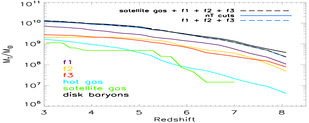
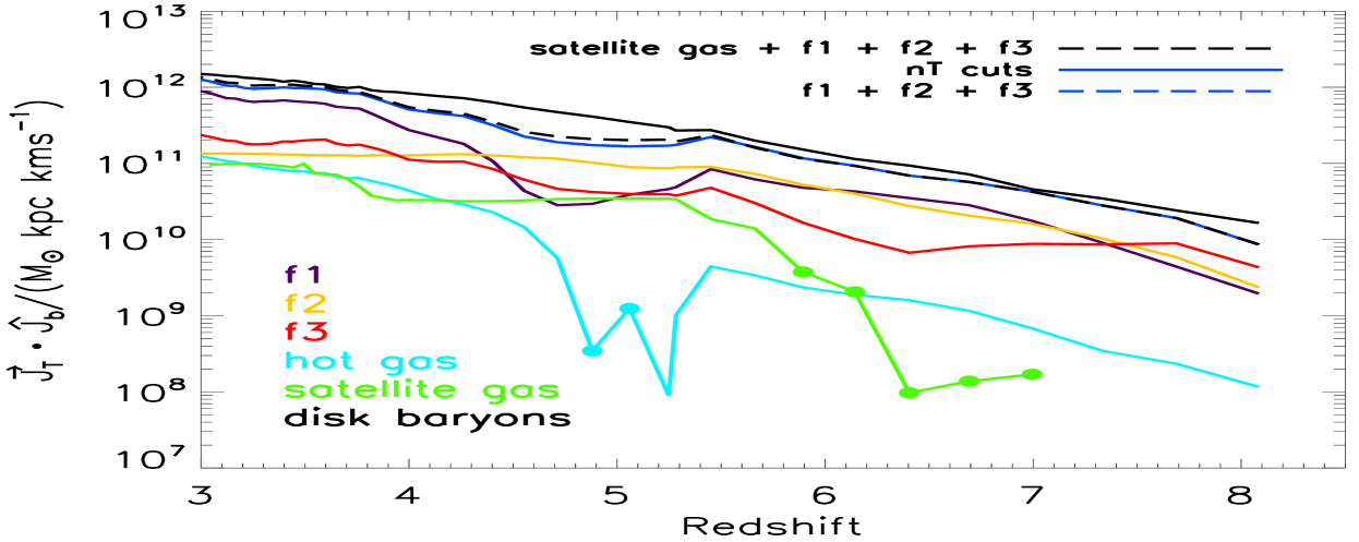
Figure 5: The relative importance of hot gas ($T>2\times 10^{5}\,$K), cold filament gas and satellite gas in establishing the mass and angular momentum budget of the central disk at high redshift. $M_{\mathrm{T}}$ (upper panel) and $\mn@boldsymbol{J}_{\mathrm{T}}$ (lower panel) have been accumulated with their corresponding signals from all prior epochs. The projection of $\mn@boldsymbol{J}_{\mathrm{T}}$ along the unit disk direction $\mn@boldsymbol{\hat{J}}_{b}$ then yields $J_{p}(z)$ in equation (14) for the filament and hot gas phases. A similar computation has been performed for the satellites, except that equations (15) and (16) have been used in place of equations (12) and (13), with the filled circles corresponding to negative $J_{p}(z)$ contributions. The dashed dark blue lines sum over the individual filament signals at each epoch, and cannot be distinguished from the solid dark blue lines, which show the accumulated signals for all of the filament gas found by applying the $nT$ cuts. The mass and angular momentum of the disk baryons defined by equations (5) and (6) have been computed at every time output and are given by the solid black lines.

The disk, filament, hot gas and satellite signals at $z_{\mathrm{in}}^{\prime}\sim 8.5$ are subtracted from their counterparts at $z<z_{\mathrm{in}}^{\prime}$ and are first recorded at $z\sim 8$ in Fig. 5 for reasons associated with the tracer colouring algorithm (which could not be applied until $z_{\mathrm{in}}\sim 10$, the earliest time output that displayed a smooth, distinct filament configuration in the NutCO run), and the subsequent trapezium integration of equations (7) and (8). This approach of shifting the origin of the entire system forward to $z_{\mathrm{in}}^{\prime}$ and modelling the $0.1r_{\mathrm{vir}}$ sphere as being empty at $z_{\mathrm{in}}^{\prime}$ is justified given: a) the desire to maintain consistency with the starting point of the tracer colouring algorithm, and; b) the negligible amount of time elapsed between $z_{1}$ (the very first output from the simulation) and $z_{\mathrm{in}}^{\prime}$ as compared to the time elapsed between $z_{1}$ and the final output at $z=3$.

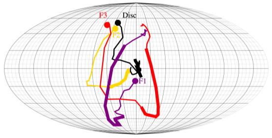
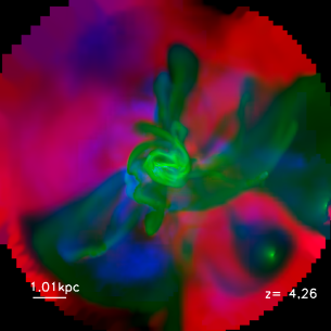
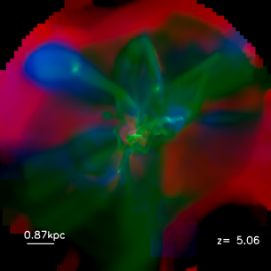
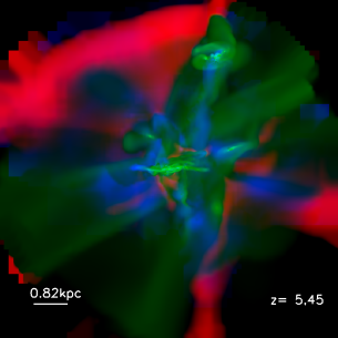
Figure 6: Top panel: A Mollweide projection of the trajectories followed by the cumulative angular momentum vectors of the disk and filaments as a function of redshift, colour coded as in Fig. 5. The filled circles indicate the starting point ($z=8$) and the thick parts of the curves mark the redshift interval $4.5\lesssim z\lesssim 5.5$ where the cumulative angular momenta of the filaments undergo a dip in Fig. 5. Bottom panels: RGB images showing the $z$-projected temperature (red channel), density (green channel), and radial velocity (blue channel) of the gas enclosed within half the virial radius of the host halo during the redshift interval $4.5\lesssim z\lesssim 5.5$. Redshifts and scales are indicated at the bottom of each panel. Note the extremely disordered gas density field at $z=5.06$ close to the (smaller) disk in the middle bottom panel, as compared to the previous (bottom right panel) and later (bottom left panel) epochs. This disorderliness is correlated with both the minimum of the dip in filament angular momentum shown in Fig. 5 and the dramatic change in the direction of the angular momenta of all the filaments visible in the top panel above.

5.1 The mass growth of the central disk component

It appears that the technical details surrounding the choice of starting point from the previous section are somewhat negligible because the upper panel of Fig. 5 indicates that the baryonic disk experiences rapid growth at high redshift, where its mass increases by a factor of $\mathord{\sim}8$ between $z\sim 8$ and $z\sim 6$. This growth is slower at later times, with a factor of $\mathord{\sim}2$ increase in disk mass between $z\sim 5$ and $z=3$. The periods of upturn in the green curves correspond to discrete luminous satellite merger events, which deposit $\mathord{\sim}1\%$ of the disk’s mass in the form of gas at early times ($z\sim 7$) and $\mathord{\sim}10\%$ at late times ($z=3$). Satellites do not therefore appreciably affect the mass budget of the disk in the redshift range $3\lesssim z\lesssim 8$. The amount of hot gas accreted onto the disk increases at a very stable rate owing to the long cooling times associated with a metal-poor intergalactic medium in the NutCO run, but by $z=3$, the hot phase only accounts for about one tenth of the disk’s accumulated mass. This phase thus plays a similarly subdominant role to the luminous satellites. Evidently the mass budget of the disk is largely controlled by the behaviour of filaments, and Fig. 5 suggests that it is the purple filament corresponding to region $1$ in the left panel of Fig. 1 that carries the most mass to the disk, typically transporting at least twice as much mass at a given epoch compared with the yellow and red filaments, whose contributions flow in approximately equal measure until $z\sim 5.5$ whereupon the purple and yellow filaments merge, with the former surviving (Fig. 2). The disappearance of the yellow filament is evident from the plateau in its accumulated mass evolution for $z\lesssim 5.5$.

By comparing the dashed black line with the solid black line in the upper panel of Fig. 5, it can be seen that the spherical flux method (which dominates the signal in equation 12), designed to predict the net radial inflow of gas accreted onto the disk, conserves mass to high precision across the disk’s evolution. This is remarkable given that the predicted flux rates across the shell could, in principle, vary quite dramatically between time intervals and hence not be well approximated by a trapezium integration. For example, it is possible that fast moving clumps of material that are accreted onto the disk pass through the thin shell undetected, which might lead one into thinking that the flux method has a systematic tendency to underestimate the accumulated mass signal. The forepart of this argument appears to hold for the very first recorded mass signal at $z\sim 8$, where the inflow of gas is just under a factor of $2$ below the disk signal in place at that epoch. Clearly this is only a phenomenon that occurs at high redshift, as it quickly becomes unimportant when the disk experiences rapid smooth growth via cold gas accretion over the subsequent time interval, which is captured by the flux method. Even so, for completeness, it is interesting to speculate on this high redshift discrepancy. One might propose that by increasing the thickness of the spherical shell from $\Delta r=1\%$ of $r_{\mathrm{vir}}$ to a larger value, there is a higher probability of capturing this apparent ‘missing’ filament mass. Yet it has been found that even when $\Delta r\sim 10\%$ of $r_{\mathrm{vir}}$ is used at the first few time outputs, there is a negligible difference in the filament (and hence filament plus satellite gas) signals. The insensitivity of the flux rate to these changes at high redshift symbolizes the robustness of the spherical flux method and implies that the offset is not caused by an underestimation of the amount of mass transported radially inward by the filaments. Given the large $100$ particle threshold imposed by the clump-finder and the technique adopted by the satellite-finding algorithm in Section 4.3.2 of identifying satellites within $0.1r_{\mathrm{vir}}$, there does appear to be some scope for suggesting that the luminous satellite component is underestimated at this epoch: less massive, darting satellites could be excluded from the light green curves in Fig. 5. After all, the satellite contributions may appear somewhat artificial in the sense that it is unlikely that there are no satellite merger events beyond $z\sim 7$. We therefore surmise that this issue could be resolved by including the contribution of satellite galaxies coming from further away than $0.1r_{\mathrm{vir}}$ at high redshift and possibly reducing the particle threshold of the clump-finder, although this latter option would impact the reliability of our satellite mass and angular momentum measurements. In light of these difficulties, and the fact that this single interval of seeming lack of mass conservation constitutes the least relevant high redshift interval in Fig. 5, further analysis probing this discrepancy is deemed unnecessary. Indeed, such an underestimate will only have a minor effect for $z\lesssim 7.5$ given the rapid rate of disk growth at early times.

5.2 Which components dominate the disk’s angular momentum budget?

The general trends of satellites and hot gas contributing a weak mass signal are also imprinted in their angular momentum evolution, shown in the lower panel of Fig. 5. At $z=3$, the hot gas signal (like the satellite signal) accounts for roughly one tenth of the disk’s accumulated angular momentum, and with the exception of its evolution between $4.5\lesssim z\lesssim 5.5$ (discussed in more detail below), increases at a steady, uniform rate towards late times. In terms of angular momentum modulus, it therefore appears that the relative contributions of the satellite and hot gas components to the disk angular momentum budget generally trace their relative disk mass contributions. In terms of angular momentum direction, the satellite material which ends up deposited onto the central disk has a tendency to be anti-aligned with respect to the disk’s angular momentum direction at high redshift, but because the signal strength is relatively weak, this mismatch only has a negligible effect. Certainly at redshifts below $z\sim 4.5$, the mass that is headed towards the disk in the satellite (and hot gas) phase appears to be more closely aligned with the disk’s direction.

When integrated across all three components (solid and dashed dark blue lines), the filament angular momentum signals show a similarly strong correlation with their corresponding mass trajectories. Clearly for the redshift ranges $3\leq z\lesssim 4$ and $5.5\lesssim z\lesssim 7.5$, the disk’s budget is driven by the transport of angular momentum from filaments. When decomposed into its individual separate trajectories, however, the cold phase shows noticeably different behaviour: (i) the yellow and red filaments transport unequal amounts of angular momentum along the disk’s direction for $z\gtrsim 4.5$, in contrast with their relative mass contributions, and; (ii) the purple and yellow filaments are equally dominant for $z\gtrsim 5.5$, unlike in the mass plot where the purple filament clearly dominates at all epochs. It should also be noted that the absence of a correlation between negative satellite signals and negative filament signals implies that satellites are not necessarily sensitive to the dynamics of the filament flow, despite often streaming along these flows (e.g. Fig. 3).

Arguably the most interesting feature of Fig. 5 is the lack of response the disk has to the sudden dip in the projected component of the purple filament’s cumulative angular momentum during the filament merger phase between $4.5\lesssim z\lesssim 5.5$. It was found that the change in the direction of the disk’s axis of rotation during successive intervals across this period was negligible (of the order a few degrees, as can be seen in the top panel of Fig. 6), and so the sharp drop-off implies that the purple filament transports angular momentum that is anti-aligned with the disk during the early phase of the merger (equation 14). The red filament’s disk-projected angular momentum contribution also abruptly changes around $z\sim 5.5$, which when combined with the purple filament’s, yields the flattened integrated dark blue curve that reflects the net small amounts of angular momentum being transported inwards by the filaments during this merger period. Looking at the bottom right and middle panels of Fig. 6, it becomes clear that this disruption is caused by the ongoing merger of the central disk with a quite massive satellite galaxy. This process leads to a complete reorganisation of the gas density field in the central region where the filaments connect to the disk, as shown in the bottom middle panel of Fig. 6. Whilst this does not affect the mass flow, as the gas must eventually pile up onto the disk in the absence of feedback and shock heating, it has dramatic consequences for the angular momentum of the gas embedded in the filaments.

One may therefore expect the new population of disk stars that form from this anti-aligned angular momentum filament material to slightly reduce the disk angular momentum growth rate that is observed in the lower panel of Fig. 5. However, a new ‘equilibrium’ configuration between filaments and disk rapidly arises, presumably through torquing (see bottom left panel of Fig. 6), in which the purple filament’s angular momentum contribution along the disk’s direction is restored. Moreover, at $z\lesssim 4$, the purple filament becomes the dominant filament contributor to the angular momentum budget by at least a factor of $\mathord{\sim}3$. This prominence is partly fuelled by the large-scale merger between the purple and yellow filaments that begins at $z\sim 5.5$ and induces a change in the mass, velocity and trajectory direction of the gas embedded within the surviving filament. Note that by $z=3$, which corresponds to the end of the simulation, the angular momentum directions of the gas present in the red and purple filaments are fairly well aligned with one another but not with the disk (see the top panel of Fig. 6), which we interpret as small-scale torquing of large-scale driven quantities.

Meanwhile, the angular momentum that our spherical flux method measures from filaments at $0.1r_{\mathrm{vir}}$ differs from the filament angular momentum deposited onto the disk during the satellite merger period because the inner dynamics within $0.1r_{\mathrm{vir}}$ are severely perturbed (note that the resultant complex inner gas trajectories appear to be imprinted in the hot gas signal too, which becomes anti-aligned in Fig. 5 around $z\sim 5$). It is likely that isothermal shocks in the disk boundary region are responsible for filtering aligned angular momentum to the disk during this phase, driving its angular momentum growth, because the baryonic disk angular momentum is dominated by its stellar component ($|\mn@boldsymbol{J}_{\star}|/|\mn@boldsymbol{J}_{\mathrm{gas}}|\sim 2.6$ at $z\sim 5$ for example), which seems to stabilise it against strong local perturbations. Should this effect apply to a large fraction of disk galaxies, one could conclude that contrary to dark matter haloes (e.g. Bett & Frenk, 2012), minor mergers of galaxies do not seem capable of significantly altering the direction of the angular momentum of the central disk.

6 Discussion

Perhaps the most defining feature of disks in galaxies with $M_{\star}\lesssim 3\times 10^{10}\,\mathrm{M}_{\sun}$ is the amount of angular momentum they possess, as it is this property that establishes many of their fundamental scaling relations such as the Tully–Fisher relation (e.g. Governato et al. 2007) and those linking velocity, metallicity, surface brightness and stellar mass (Dekel & Woo, 2003; Dekel & Birnboim, 2006). The Tully–Fisher relation, in particular, is an important constraint that many semi-analytic models of galaxy formation strive to satisfy (Hatton et al., 2003; Cattaneo et al., 2006; Croton et al., 2006; De Lucia et al., 2006). Understanding how the disk acquires its angular momentum is hence of central importance, and has been the subject of this paper.

6.1 The dominance of filaments at high redshift

The evidence favouring the growth of disks in low mass systems via a mode of cold gas accretion appears to be mounting. Kereš et al. (2005) performed SPH simulations of several hundred galaxies between $0\leq z\leq 3$ using a comoving gravitational softening scale of $5\,h^{-1}\,$kpc, and found evidence of a clear shift in the total fraction of gas accreted with temperatures $T<2.5\times 10^{5}\,$K around a galaxy stellar mass of $M_{\star}\sim 2.5\times 10^{10}\,\mathrm{M_{\sun}}$, with at most a factor of $\mathord{\sim}1.6$ deviation in $M_{\star}$ across this redshift range. Ocvirk et al. (2008) conducted a similar statistical analysis on haloes from the HORIZON-MARENOSTRUM simulation with $10^{10}<M_{\mathrm{H}}/\mathrm{M}_{\sun}<10^{13}$ at higher redshifts between $2\leq z\leq 5$, in an attempt to measure the temperature and density of the gas deposited onto the central galaxies of these systems, which were simulated using the RAMSES code at a physical resolution scale of $\sim 1h^{-1}\,$kpc. Their results demonstrated that the fraction of gas accreted at temperatures $T<2.5\times 10^{5}\,$K sharply increases for $M_{\mathrm{H}}\lesssim 4\times 10^{11}\,\mathrm{M}_{\sun}$, in concordance with the estimates provided by Birnboim & Dekel (2003) and Kereš et al. (2005). By resolving and examining the various components of the filamentary gas phase across a wide range in redshift, the results from Fig. 5 in this paper provide quantitive support for the cold mode paradigm of gas accretion onto a Milky Way like disk, advocated by the above studies. They also show that a single filament can be responsible for driving the mass budget of the baryonic disk, although this does not necessarily map to a dominance of the disk’s angular momentum budget, as two filaments appear to closely share priority at the higher redshifts ($z\gtrsim 5.5$), despite a clear difference in their mass contributions. The flow of cold gas onto the central disk is not necessarily a smooth, continuous process either. While satellites do not significantly perturb the filament trajectories in general (except in the region close to the central disk, and even then, not very often and only over short periods of time), large-scale motions of filaments can lead to mergers between these cold streams (Pichon et al., 2011) and this process is able to change the orientation of angular momentum advected along these flows, probably even if gas channelled along each of the filament mergers in question is co-planar with the disk’s rotation before the merger.

A quantitative result of this kind has remained elusive to many previous studies mostly due to the parsec-scale physical resolution required to resolve the satellites, filaments and disk components within the inner tenth of the virial region at $z>3$. Some authors have recently started to probe this resolution barrier, however. Kimm et al. (2011) measured the angular momentum of gas in radial bins as a function of redshift, for the same resimulated NUT Milky Way like halo analyzed in this paper. Upon stacking the radial profiles in two separate redshift regimes ($z\leq 3$ and $z>3$), they found evidence for a sudden loss in the amount of specific angular momentum transported by gas in the $0.1r_{\mathrm{vir}}$ region, but with a physical resolution scale of only $\mathord{\sim}50\,$pc, were unable to speculate on the cause of this loss. Although the analysis in this paper does not address this issue per se, it does show that the filaments supply enough angular momentum to the boundary of the disk region to be able to account for the angular momentum locked-up in the disk across most epochs at $z>3$, a result that has been found by using a filament tracer colouring technique.

Several studies have also demonstrated that the angular momentum vectors of dark matter and gas are not necessarily aligned within the virial region of galaxies at both low ($z=0$) and high ($z\leq 3$) redshift (Bett et al., 2010; Roškar et al., 2010). Danovich et al. (2012) reported a weak correlation between the angular momentum direction of gas in the inner ($\mathord{\sim}0.1r_{\mathrm{vir}}$) and outer ($\mathord{\sim}1r_{\mathrm{vir}}$) galaxy regions at $z=2.5$, and a large body of evidence has now been presented that confirms the existence of mismatches in gas angular momentum directions over scales of a few disk scalelengths, giving rise to the population of ‘warped’ disks (García-Ruiz et al., 2002; Shen & Sellwood, 2006). Despite being observed as a low redshift phenomena, the recent simulation study by Roškar et al. (2010) has argued that warps may exist around $z\sim 2\mbox{--}3$. In Fig. 5 of this paper, the amount of angular momentum transported along the disk’s direction by all the filaments is comparable to that locked-up in the disk, which would not be the case if large-scale misaligned signals reported above were preserved at the disk boundary. If the claim that the directions of the gas angular momentum vectors vary with distance from the central galaxy holds across the galaxy’s lifetime, some physical mechanism must be responsible for aligning the infalling angular momentum at the disk’s edge. For example, Roškar et al. (2010) have argued that freshly accreted gas at the virial radius is strongly torqued by the hot halo gas component, and cited this as a possible cause of the warps between inner and outer disk structure. Whilst hot gas torques are unlikely to be dominant in our case, it is nevertheless surmised that shocks and/or torques remove the components of the purple filament’s velocity that are misaligned with respect to the disk’s plane of rotation, thereby explaining why this filament is able to maintain a relatively stable transfer of aligned angular momentum to the disk between $3\lesssim z\lesssim 8$.

Despite the evidence from both Fig. 5 and the aforementioned simulation studies favouring the cold gas paradigm, not all authors are convinced that this phase is quite so dominant in growing the disk components of low mass galaxies. Murante et al. (2012) monitored the fractional accretion rate onto two Milky Way like haloes and found that $\mathord{\sim}50\%$ of the accreted gas onto the central galaxy between $3\leq z\leq 6$ was in a warm phase, with a temperature in the range $2.5\times 10^{5}<T/\mathrm{K}<10^{6}$. They attributed this apparent discrepancy to a supernovae feedback prescription that only modelled thermal heating, as opposed to thermal and kinetic heating. The effects of supernovae feedback on filament structure were also examined by van de Voort et al. (2011), who suggested that it reduces the growth rate of low mass central galaxies residing in haloes with mass $M_{\mathrm{H}}\lesssim 10^{12}\,\mathrm{M}_{\sun}$, implying that the filaments streaming cold gas at large inflow rates in Fig. 5 do not survive when supernovae feedback is included. Powell et al. (2011), however, argued that this result is probably an artefact of supernovae feedback implementation, because with individual Sedov–Taylor blasts from the ultra-high resolution ($\Delta x_{\mathrm{res}}\sim 0.5\,$pc) NUT feedback run simulation, the net mass inflow rates of gas in the filament phase were found to be an order of magnitude larger than the supernovae-driven mass outflow rates. The Powell et al. (2011) study hence implies that whilst the spatial distribution of filaments local to the disk is likely to be perturbed around sites of intensive stellar explosions, the amount of filament gas flowing towards the disk should largely be unaltered. Therefore, the amount of angular momentum aligned with the disk that is transported by filaments is probably unchanged too, given the general correlation between the filament mass and disk-projected angular momentum signals in Fig. 5. It is therefore expected that the difference between the supernovae feedback version of Fig. 5 and its counterpart presented in this paper is not significant, but we leave this comparison as a future exercise.

6.2 Understanding the impact of mergers

Fig. 5 shows that luminous satellite mergers constitute only a minor fraction of the disk’s mass and angular momentum modulus between $3\lesssim z\lesssim 8$. This result does not necessarily imply, however, that satellites as a general population have little effect on the disk’s evolution. Bett & Frenk (2012) analyzed present day Milky Way haloes of mass $M_{\mathrm{H}}\sim 10^{12}\mbox{--}10^{12.5}\,h^{-1}\,\mathrm{M}_{\sun}$ from one of the Millennium Simulation runs and examined the importance of ‘spin flips’, which are defined as abrupt changes of more than $45^{\circ}$ in the orientation of a component’s angular momentum vector. They argued that over $90\%$ of their detected host halo spin flips were caused by minor mergers, and demonstrated that the number of flip events increases in the inner halo where the central galaxy resides. They further speculated that these spin flips could destroy the host’s stellar disk (which is included in the baryonic disk signal of Fig. 5), or torque it (see, for example, Ostriker & Binney 1989). In both of these scenarios, one would expect a change in the angular momentum direction of the baryonic disk component. The validity of this hypothesis remains an open question because the existence of a simple correlation between dark halo spin flips and disk spin flips is yet to be confirmed: several recent studies have in fact hinted at a lack of correlation between the two (Scannapieco et al., 2009; Stinson et al., 2010; Sales et al., 2011). It will be interesting to test in more detail whether this claim by Bett & Frenk (2012) holds for the NUT host halo in this study, which experiences multiple minor mergers across its accretion history (as indicated by Fig. 3). However, we suggest that it is highly unlikely since the top panel of Fig. 6 clearly shows that the angular momentum direction of the disk varies very little throughout the majority of its lifetime.

6.3 High redshift contributions to the present day mass and angular momentum of the disk from the NutCO run

It is also informative to estimate the fraction of the disk’s mass and angular momentum at $z=0$ that is already in place at $z=3$, as large high redshift contributions would further highlight the importance of understanding the primordial phase of Milky Way like galaxy growth. Crude estimates are hence provided in this section, but it should be noted that more rigorous measurements could be made by analyzing all of the lower resolution outputs from the NutCO run between $0\leq z\leq 3$ and extending Fig. 5 to $z=0$.

Kimm et al. (2011) measured the total amount of baryonic mass (gas plus stars) within $0.1r_{\mathrm{vir}}$ from the $\Delta x_{\mathrm{min}}=48\,$pc NutCO run at $z=0$ and found that $M_{b}(z=0)\sim 8\times 10^{10}\,\mathrm{M}_{\sun}$. This measurement includes the central contributions from all of the gas phases (satellite, hot mode, cold mode and disk) and all of the stars (satellite, disk and bulge), and is a factor of $\mathord{\sim}6$ greater than the baryonic disk signal at $z=3$ from Fig. 5, which is $M_{b}(z=3)\sim 1.3\times 10^{10}\,\mathrm{M}_{\sun}$. Multiplying the modulus of the total baryonic specific angular momentum contributions within the $0.1r_{\mathrm{vir}}$ region at $z=0$ from the Kimm et al. (2011) study by the relevant component masses yields an estimate of the total baryonic angular momentum signal: $J_{b}(z=0)\sim 4.4\times 10^{13}\,\mathrm{M}_{\sun}\,\mathrm{kpc}\,\mathrm{km\,s^{-1}}$. This is a factor of $\mathord{\sim}30$ higher than the modulus of the baryonic disk angular momentum signal at $z=3$ shown in Fig. 5: $J_{b}(z=3)\sim 1.6\times 10^{12}\,\mathrm{M}_{\sun}\,\mathrm{kpc}\,\mathrm{km\,s^{-1}}$. Note that the mass (and most probably the angular momentum) ratios are upper limit estimates because the Kimm et al. (2011) measurements include the satellite star and non-disk gas contributions, whereas Fig. 5 just shows the baryonic disk signals defined according to equations (5) and (6).

In summary, at least $\mathord{\sim}16\%$ ($\mathord{\sim}4\%$) of the NUT disk’s final mass (angular momentum) is already in place by $z=3$, suggesting that high redshift epochs studied in this paper represent a non-negligible period of the disk’s accretion history.

7 Conclusions

We have analyzed an Adaptive Mesh Refinement cosmological resimulation with $12\,$pc resolution in order to address whether the angular momentum acquired by the baryonic disk of a Milky Way like galaxy at $z\geq 3$ is driven by filaments. The filaments have been identified by tagging Lagrangian tracer particles within a region of length $2r_{\mathrm{vir}}$ from the disk’s centre at each epoch. The method assigns one of three colours (one for each filament) to the tracer particles by using a nearest neighbours scheme, and subsequently locates the ‘pure’ cells within the spherical grid of radius $2r_{\mathrm{vir}}$ that contain tracer particles of identical colour. Individual filament trajectories are then grown around these pure sites. A satellite finding algorithm has also been presented, which operates under the principle that a given satellite substructure of the main host at time $t$ has at some earlier time been a separate field galaxy of its own. With the filaments and satellites resolved, the aim of this paper has been to measure their contributions to the host’s disk angular momentum budget at each epoch. For the filament and hot gas components, the mass and angular momentum transported to the central disk has been computed by recording both the net inward flux across an outwardly propagating spherical shell on the disk’s edge at $0.1r_{\mathrm{vir}}$, and the contribution from the material swept up by the shell’s outward radial motion. Satellite signals have been measured by adopting an alternative technique that pinpoints mergers with the disk and records their angular momentum at the final pre-accretion stage. The results suggest that:

• The cumulative effect of the cold filament gas phase dominates the mass and angular momentum budgets of the disk as a function of time, hence providing quantitative support for the cold gas paradigm of disk growth in low mass galaxies at high redshift.

• For $5.5\lesssim z\lesssim 7.5$, the largest portion of the filament angular momentum signal is transported by two filaments, which start to merge around $z\sim 5.5$. This is accompanied by the central disk merging with a satellite galaxy, which temporarily induces a dramatic change in the orientation of the angular momentum transported towards the disk, but the surviving filament remnant quickly realigns itself along the direction imposed by the large-scale flow and by $z\sim 4$ dominates the filament angular momentum budget by at least a factor of $3$.

• The luminous satellites account for at most one tenth of the disk mass and angular momentum modulus at any given epoch.

Appendix A Identifying the filaments using tracer particles

A.1 The algorithm

The tracer propagation method, first encountered in Section 3.2, consists of three principal stages:

1. Colouring the tracer particles across time. At some initial early time $t_{1}$ ($z_{1}\sim 10$), planar cuts are used to divide the filaments into distinct regions within a spherical grid $\mathcal{G}_{2.0}$ of radius $2r_{\mathrm{vir}}$ (black planes in the left panel of Fig. 1). Each region is assigned a unique colour and tracer particles are initially coloured according to the region in which they reside. Hence there is a single filament per region by construction, and we refer to the filaments in regions $1,2$, and $3$ of the left panel of Fig. 1 as the purple, yellow and red filaments respectively.

   The Lagrangian nature of the system poses two computational difficulties when assigning colour:

   • filaments mix in the vicinity of the disk (as can be seen in the right panel of Fig. 1), and;

   • filaments acquire a drift velocity on scales $r\gtrsim r_{\mathrm{vir}}$ (Pichon et al., 2011), which can lead to them switching between regions within $r_{\mathrm{vir}}$ as the host grows.

   

   

   

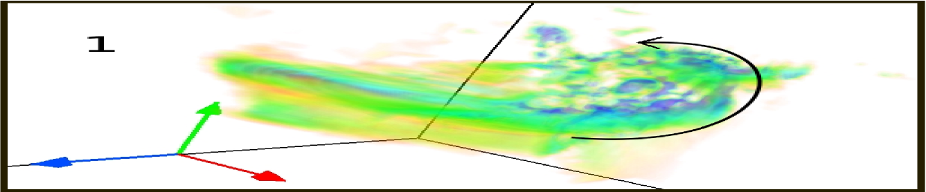
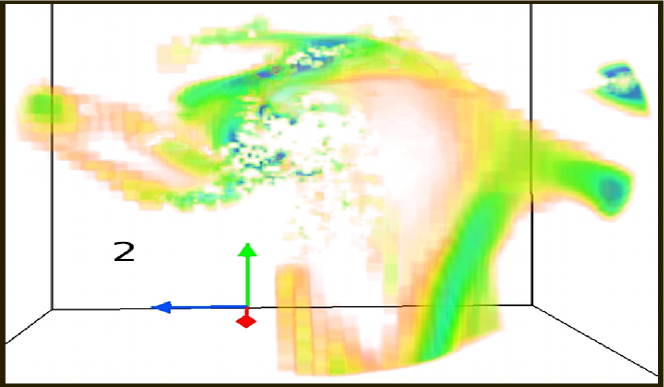
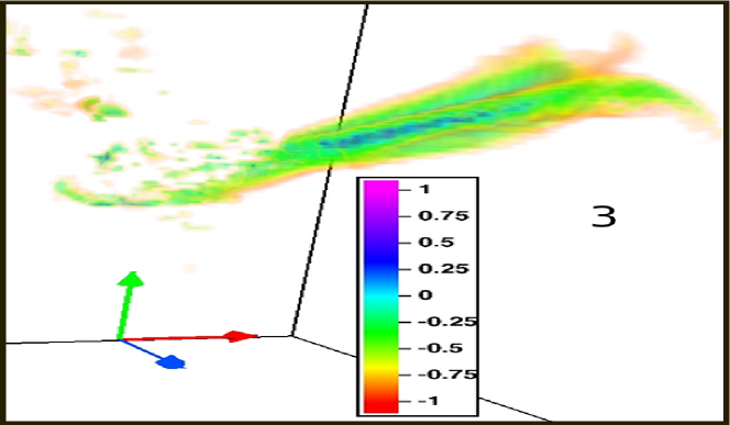
   Figure 7: These VAPOR images illustrate the trajectories of each gas filament on $\mathcal{G}_{0.5}$ ($r_{\mathrm{vir}}\sim 7.5\,$kpc) at $z\sim 8$ in the NutCO run with $\ell=17$ ($\Delta x\sim 12\,$pc), as identified by the colour propagation technique. Each panel corresponds to the updated versions of the purple, yellow and red filaments associated with regions $1,2$ and $3$ respectively in the left panel of Fig. 1, and follows the same density colour scaling as in previous figures. The black curved arrow in the top panel indicates the gas flow direction of the purple filament.

   The first issue is tackled by resolving the filament trajectories at the following time output $t_{2}$, by which time the vast majority of the incorrectly coloured particles within $0.1r_{\mathrm{vir}}$ at $t_{1}$ have accreted onto the disk during the $\Delta t=t_{2}-t_{1}$ interval, and are therefore no longer associated with a filament. To circumvent the second issue, previously flagged tracer particles $i$ at locations $\mn@boldsymbol{r}_{i}(t_{1})$ that have moved during the $\Delta t$ interval are updated according to their new instantaneous locations $\mn@boldsymbol{r}_{i}(t_{2})$ at the following time $t_{2}$, provided that they coincide with filament cells at $t_{2}$. All of the newly accreted tracer particles that are co-spatial with filaments within the (larger) host spherical region at $t_{2}$ that have not been assigned a colour are then given a colour according to their host region. At subsequent time outputs $t_{j}$ ($t_{3}$ onwards), the newly accreted tracer particles are instead assigned the majority colour of their $N$ nearest coloured tracer neighbours that sample the filaments at $\mn@boldsymbol{r}_{i}(t_{j})$ ($N$ was at least $100$). Note that the above neighbouring scheme cannot be used for $t_{2}$ because the constructed filament trajectories are not known until the end of the time output (see steps $2$ and $3$ below).

2. Colouring the grid. Once all of the filament tracer particles within $\mathcal{G}_{2.0}$ are coloured, the overall colours of the member tracer cells are determined (particles located in non-filament cells within $r_{\mathrm{vir}}$ are ignored, so that only filaments are resolved). The prescription used in this study enforces the condition that each coloured tracer cell is ‘pure’, consisting entirely of particles with identical colour. The advantage of this approach is that it avoids the use of ad hoc criteria to help decide the overall colour of a cell that contains a certain ratio of particles of different colours.

3. Individual filament growth. The final step propagates the pure cell colours to neighbouring uncoloured filament cells within $\mathcal{G}_{2.0}$. Filaments are simultaneously grown around the cells with pure colour and the procedure terminates once all neighbours of neighbours etc, are coloured and the only remaining neighbouring cells are non-filament cells or cells that already have a colour.

A.2 Uncertainties

While the $nT$ cuts are only approximate, Powell et al. (2011) have argued that the associated uncertainties in the bulk physical properties of the filaments (average mass, velocity etc) remain very small because: (i) these cuts successfully capture the dense core of the filaments (as confirmed by visual verification) around the disk in the NUT suite runs with $\Delta x_{\mathrm{res}}=0.5\,$pc, and; (ii) reducing the lower density threshold has little impact on these properties. Hence we also ignore the uncertainties associated with the $nT$ criteria in what follows, and the constructed filaments are calibrated against their $nT$ counterparts.

The uncertainties introduced by the filament colour propagation scheme can be of two types:

1. not attributing any colour to a valid filament cell, and;

2. attributing the wrong colour to a filament cell.

The relative importance of uncertainties of type (i) was assessed by recording the number of filament cells without a colour upon application of the propagation method, as a fraction of the total number of filament cells found by applying the $nT$ criteria, for different grid sizes at $z\geq 3$ in the NutCO run. These uncertainties were measured to be below the percent level at all times.

Type (ii) uncertainties are now examined. Since the aim of this paper is to quantify the amount of angular momentum transferred to the disk by filaments, it is key that the trajectories of these cold flows in the disk’s vicinity are reconstructed to a high level of precision. The filament reconstruction stage (step $3$ of the colour propagation algorithm) was hence repeated over the $0.15r_{\mathrm{vir}}$ region to ensure that the angular momentum calculations around the disk were performed at the resolution limit (this particular choice of grid radius is justified in Section 4.3.1). Once constructed, it is natural to wonder whether the filament trajectories are representative of their ‘true’ counterparts in the simulation. A rigorous quantification of the relative discrepancies has proven elusive, so we provide the reader with a powerful qualitative diagnostic instead: a computer assisted visual check where the filament density field identified by the tracer colouring algorithm is compared to calculated flow lines. Fig. 7 shows $3$D images of the density of each filament from the right panel of Fig. 1, as found by implementing the colour propagation technique on $\mathcal{G}_{0.5}$ with spacing $\Delta x\sim 12\,$pc at $z\sim 8$. By zooming into the larger $0.5r_{\mathrm{vir}}$ region at the resolution limit, it is possible to test the algorithm’s ability to follow each filament onto the disk. The viewing angle in each panel of Fig. 7 has been rotated to demonstrate the nature of the individual trajectories, and varies from filament to filament. By comparison with the right panel of Fig. 1, it is clear from Fig. 7 that the separate filament paths are correctly identified to the point of disk contact, and that the curvature about the disk region is particularly well-resolved, which is most evident for the yellow filament in region $2$. Note that the sudden upturn of the red filament’s inner trajectory in Fig. 1 after mixing in the central region is also captured by the colour propagation routine. Thus Fig. 7 strongly suggests that the algorithm is able to successfully construct the trajectories of individual filaments even though, contrary to type (i) uncertainties, it is difficult to argue that it does so at the percent level accuracy.

Appendix B Pinpointing the satellites

The details of the satellite-finding algorithm introduced in Section 3.3 are provided in this Appendix.

In this study, a substructure $i$ that is classed as a satellite of the host at a given time output $t_{i}$ satisfies both of the following criteria:

• it partially or fully infringes the host’s virial sphere at $t_{i}$, and;

• it has previously been a halo.

The former condition ensures that only substructures within the host’s virial region are considered, and is hence satisfied should any region within satellite $i$’s virial radius also be contained by the host’s virial sphere. If it is, then $i$ is flagged as a satellite candidate, otherwise it is skipped. Assuming $i$ is a satellite candidate, the latter condition involves computing its merger tree, and if at any time output along its main branch one of its main progenitors becomes a halo, then $i$ is flagged as a satellite.

In order to compute the main branch along $i$’s merger tree, the progenitor that donates the most mass to $i$ is identified: this progenitor, $j$, is called the ‘main progenitor’, and the link from $i$ to $j$ is referred to as the ‘main branch’ (following Tillson et al. 2011). The satellite-finding algorithm imposes the condition that in order for a subhalo to be a satellite at time $t$, it must have been a field halo at some point earlier in its merger history. Note that this method allows objects to share the same main progenitor and hence maximizes the number of possible satellites, resulting in the purest filamentary angular momentum signals once the central satellite galaxy regions have been masked according to the prescription in Section 3.3.

REFERENCES

- Aragón-Calvo et al. (2010) Aragón-Calvo M. A., van de Weygaert R., Jones B. J. T., 2010, MNRAS, 408, 2163
- Aubert & Pichon (2007) Aubert D., Pichon C., 2007, MNRAS, 374, 877
- Bett et al. (2010) Bett P., Eke V., Frenk C. S., Jenkins A., Okamoto T., 2010, MNRAS, 404, 1137
- Bett & Frenk (2012) Bett P. E., Frenk C. S., 2012, MNRAS, 420, 3324
- Binney (1977) Binney J., 1977, ApJ, 215, 483
- Birnboim & Dekel (2003) Birnboim Y., Dekel A., 2003, MNRAS, 345, 349
- Bond et al. (1996) Bond J. R., Kofman L., Pogosyan D., 1996, Nature, 380, 603
- Book et al. (2011) Book L. G., Brooks A., Peter A. H. G., Benson A. J., Governato F., 2011, MNRAS, 411, 1963
- Brooks et al. (2009) Brooks A. M., Governato F., Quinn T., Brook C. B., Wadsley J., 2009, ApJ, 694, 396
- Bullock et al. (2001) Bullock J. S., Kolatt T. S., Sigad Y., Somerville R. S., Kravtsov A. V., Klypin A. A., Primack J. R., Dekel A., 2001, MNRAS, 321, 559
- Cattaneo et al. (2006) Cattaneo A., Dekel A., Devriendt J., Guiderdoni B., Blaizot J., 2006, MNRAS, 370, 1651
- Croton et al. (2006) Croton D. J., Springel V., White S. D. M., De Lucia G., Frenk C. S., Gao L., Jenkins A., Kauffmann G., Navarro J. F., Yoshida N., 2006, MNRAS, 365, 11
- Dalcanton et al. (1997) Dalcanton J. J., Spergel D. N., Summers F. J., 1997, ApJ, 482, 659
- Danovich et al. (2012) Danovich M., Dekel A., Hahn O., Teyssier R., 2012, MNRAS, p. 2777
- de Jong (1996) de Jong R. S., 1996, A&A, 313, 377
- de Jong & Lacey (2000) de Jong R. S., Lacey C., 2000, ApJ, 545, 781
- De Lucia et al. (2006) De Lucia G., Springel V., White S. D. M., Croton D., Kauffmann G., 2006, MNRAS, 366, 499
- Dekel & Birnboim (2006) Dekel A., Birnboim Y., 2006, MNRAS, 368, 2
- Dekel et al. (2009) Dekel A., Birnboim Y., Engel G., Freundlich J., Goerdt T., Mumcuoglu M., Neistein E., Pichon C., Teyssier R., Zinger E., 2009, Nature, 457, 451
- Dekel & Woo (2003) Dekel A., Woo J., 2003, MNRAS, 344, 1131
- Devriendt et al. (2010) Devriendt J., Rimes C., Pichon C., Teyssier R., Le Borgne D., Aubert D., Audit E., Colombi S., Courty S., Dubois Y., Prunet S., Rasera Y., Slyz A., Tweed D., 2010, MNRAS, 403, L84
- Doroshkevich (1970) Doroshkevich A. G., 1970, Astrophysics, 6, 320
- Dubois et al. (2012) Dubois Y., Pichon C., Haehnelt M., Kimm T., Slyz A., Devriendt J., Pogosyan D., 2012, MNRAS, 423, 3616
- Dunkley et al. (2009) Dunkley J., Komatsu E., Nolta M. R., Spergel D. N., Larson D., Hinshaw G., Page L., Bennett C. L., Gold B., Jarosik N., Weiland J. L., Halpern M., Hill R. S., Kogut A., Limon M., Meyer S. S., Tucker G. S., Wollack E., Wright E. L., 2009, ApJS, 180, 306
- Fall & Efstathiou (1980) Fall S. M., Efstathiou G., 1980, MNRAS, 193, 189
- Fardal et al. (2001) Fardal M. A., Katz N., Gardner J. P., Hernquist L., Weinberg D. H., Davé R., 2001, ApJ, 562, 605
- Faucher-Giguère et al. (2010) Faucher-Giguère C.-A., Kereš D., Dijkstra M., Hernquist L., Zaldarriaga M., 2010, ApJ, 725, 633
- Faucher-Giguère et al. (2011) Faucher-Giguère C.-A., Kereš D., Ma C.-P., 2011, MNRAS, 417, 2982
- Fumagalli et al. (2011) Fumagalli M., Prochaska J. X., Kasen D., Dekel A., Ceverino D., Primack J. R., 2011, MNRAS, 418, 1796
- García-Ruiz et al. (2002) García-Ruiz I., Sancisi R., Kuijken K., 2002, A&A, 394, 769
- Gogarten et al. (2010) Gogarten S. M., Dalcanton J. J., Williams B. F., Roškar R., Holtzman J., Seth A. C., Dolphin A., Weisz D., Cole A., Debattista V. P., Gilbert K. M., Olsen K., Skillman E., de Jong R. S., Karachentsev I. D., Quinn T. R., 2010, ApJ, 712, 858
- Governato et al. (2007) Governato F., Willman B., Mayer L., Brooks A., Stinson G., Valenzuela O., Wadsley J., Quinn T., 2007, MNRAS, 374, 1479
- Haardt & Madau (1996) Haardt F., Madau P., 1996, ApJ, 461, 20
- Hahn et al. (2007) Hahn O., Porciani C., Carollo C. M., Dekel A., 2007, MNRAS, 375, 489
- Hatton et al. (2003) Hatton S., Devriendt J. E. G., Ninin S., Bouchet F. R., Guiderdoni B., Vibert D., 2003, MNRAS, 343, 75
- Hoyle (1951) Hoyle F., 1951, in Problems of Cosmical Aerodynamics The Origin of the Rotations of the Galaxies. p. 195
- Kay et al. (2000) Kay S. T., Pearce F. R., Jenkins A., Frenk C. S., White S. D. M., Thomas P. A., Couchman H. M. P., 2000, MNRAS, 316, 374
- Kereš et al. (2009) Kereš D., Katz N., Fardal M., Davé R., Weinberg D. H., 2009, MNRAS, 395, 160
- Kereš et al. (2005) Kereš D., Katz N., Weinberg D. H., Davé R., 2005, MNRAS, 363, 2
- Kimm et al. (2011) Kimm T., Devriendt J., Slyz A., Pichon C., Kassin S. A., Dubois Y., 2011, Preprint (arXiv:1106.0538)
- Krumholz & Tan (2007) Krumholz M. R., Tan J. C., 2007, ApJ, 654, 304
- MacArthur et al. (2004) MacArthur L. A., Courteau S., Bell E., Holtzman J. A., 2004, ApJS, 152, 175
- Mo et al. (1998) Mo H. J., Mao S., White S. D. M., 1998, MNRAS, 295, 319
- Monaghan & Lattanzio (1985) Monaghan J. J., Lattanzio J. C., 1985, A&A, 149, 135
- Muñoz-Mateos et al. (2007) Muñoz-Mateos J. C., Gil de Paz A., Boissier S., Zamorano J., Jarrett T., Gallego J., Madore B. F., 2007, ApJJ, 658, 1006
- Murante et al. (2012) Murante G., Calabrese M., De Lucia G., Monaco P., Borgani S., Dolag K., 2012, ApJL, 749, L34
- Navarro et al. (1995) Navarro J. F., Frenk C. S., White S. D. M., 1995, MNRAS, 275, 720
- Ocvirk et al. (2008) Ocvirk P., Pichon C., Teyssier R., 2008, MNRAS, 390, 1326
- Ostriker & Binney (1989) Ostriker E. C., Binney J. J., 1989, MNRAS, 237, 785
- Peebles (1969) Peebles P. J. E., 1969, ApJ, 155, 393
- Pichon et al. (2011) Pichon C., Pogosyan D., Kimm T., Slyz A., Devriendt J., Dubois Y., 2011, MNRAS, p. 1739
- Pogosyan et al. (1998) Pogosyan D., Bond J. R., Kofman L., 1998, JRASC, 92, 313
- Powell et al. (2011) Powell L. C., Slyz A., Devriendt J., 2011, MNRAS, 414, 3671
- Prunet et al. (2008) Prunet S., Pichon C., Aubert D., Pogosyan D., Teyssier R., Gottloeber S., 2008, ApJS, 178, 179
- Rasera & Teyssier (2006) Rasera Y., Teyssier R., 2006, A&A, 445, 1
- Rosdahl & Blaizot (2012) Rosdahl J., Blaizot J., 2012, MNRAS, p. 2837
- Roškar et al. (2010) Roškar R., Debattista V. P., Brooks A. M., Quinn T. R., Brook C. B., Governato F., Dalcanton J. J., Wadsley J., 2010, MNRAS, 408, 783
- Sales et al. (2011) Sales L. V., Navarro J. F., Cooper A. P., White S. D. M., Frenk C. S., Helmi A., 2011, MNRAS, 418, 648
- Scannapieco et al. (2009) Scannapieco C., White S. D. M., Springel V., Tissera P. B., 2009, MNRAS, 396, 696
- Schmidt (1959) Schmidt M., 1959, ApJ, 129, 243
- Shen et al. (2006) Shen J., Abel T., Mo H. J., Sheth R. K., 2006, ApJ, 645, 783
- Shen & Sellwood (2006) Shen J., Sellwood J. A., 2006, MNRAS, 370, 2
- Sousbie (2011) Sousbie T., 2011, MNRAS, 414, 350
- Steidel et al. (2010) Steidel C. C., Erb D. K., Shapley A. E., Pettini M., Reddy N., Bogosavljević M., Rudie G. C., Rakic O., 2010, ApJ, 717, 289
- Stinson et al. (2010) Stinson G. S., Bailin J., Couchman H., Wadsley J., Shen S., Nickerson S., Brook C., Quinn T., 2010, MNRAS, 408, 812
- Sutherland & Dopita (1993) Sutherland R. S., Dopita M. A., 1993, ApJS, 88, 253
- Teyssier (2002) Teyssier R., 2002, A&A, 385, 337
- Tillson et al. (2011) Tillson H., Miller L., Devriendt J., 2011, MNRAS, p. 1293
- Tweed et al. (2009) Tweed D., Devriendt J., Blaizot J., Colombi S., Slyz A., 2009, A&A, 506, 647
- van de Voort et al. (2011) van de Voort F., Schaye J., Booth C. M., Haas M. R., Dalla Vecchia C., 2011, MNRAS, 414, 2458
- van den Bosch et al. (2002) van den Bosch F. C., Abel T., Croft R. A. C., Hernquist L., White S. D. M., 2002, ApJ, 576, 21
- White (1984) White S. D. M., 1984, ApJ, 286, 38
- White & Rees (1978) White S. D. M., Rees M. J., 1978, MNRAS, 183, 341