Cosmological MHD Simulations of Galaxy Cluster Radio Relics: Insights and Warnings for Observations

Abstract

Non-thermal radio emission from cosmic ray electrons in the vicinity of merging galaxy clusters is an important tracer of cluster merger activity, and is the result of complex physical processes that involve magnetic fields, particle acceleration, gas dynamics, and radiation. In particular, objects known as radio relics are thought to be the result of shock-accelerated electrons that, when embedded in a magnetic field, emit synchrotron radiation in the radio wavelengths. In order to properly model this emission, we utilize the adaptive mesh refinement simulation of the magnetohydrodynamic evolution of a galaxy cluster from cosmological initial conditions. We locate shock fronts and apply models of cosmic ray electron acceleration that are then input into radio emission models. We have determined the thermodynamic properties of this radio-emitting plasma and constructed synthetic radio observations to compare to observed galaxy clusters. We find a significant dependence of the observed morphology and radio relic properties on the viewing angle of the cluster, raising concerns regarding the interpretation of observed radio features in clusters. We also find that a given shock should not be characterized by a single Mach number. We find that the bulk of the radio emission comes from gas with $\mathrm{T}>5\times 10^{7}\mathrm{K}$, $\mathrm{\rho}\sim 10^{-28}-10^{-27}\mathrm{g/cm^{3}}$, with magnetic field strengths of $0.1-1.0\mathrm{\mu G}$ and shock Mach numbers of $\mathcal{M}\sim 3-6$. We present an analysis of the radio spectral index which suggests that the spatial variation of the spectral index can mimic synchrotron aging. Finally, we examine the polarization fraction and position angle of the simulated radio features, and compare to observations.

1. Introduction

Galaxy clusters are hosts to a variety of thermal and non-thermal phenomena, many of which are the result of cosmological structure formation. The study of relativistic particles in galaxy cluster environments was motivated by the observation of the radio halo in the Coma cluster by Large et al. (1959), and has since grown into an industry of observations, theory, and simulation. For a review on current radio observations of galaxy clusters see Ferrari et al. (2008); Feretti et al. (2012), and for a review on the non-thermal processes see Dolag et al. (2008). Here we review the basic characteristics of galaxy cluster radio “halos” and giant radio “relics,” to use the classification in Ferrari et al. (2008). Radio halos are usually $\sim\mathrm{Mpc-}$sized features in galaxy clusters, closely following the X-ray morphology in the central regions of the cluster. They are generally characterized by very low ($<$ few percent) linear polarization fractions, and are found in galaxy clusters with disturbed morphology and no evidence for a cool core (Ferrari et al., 2008; Giovannini et al., 2009; Feretti et al., 2012). The origin of the emission is thought to be from relativistic ($\gamma\sim 10^{4}$) electrons emitting synchrotron radiation. The source of the energy in these electrons, however, is debated. It may originate from the decay of pions (the “secondary” or “hadronic” model), created by interactions between cosmic ray protons and the thermal population (Dennison, 1980; Dolag & Enßlin, 2000; Miniati et al., 2001), which would be strengthened by the observation of gamma-ray emission in cluster cores. However, initial studies of many galaxy clusters using the FERMI satellite (Ackermann et al., 2010), as well as for fewer objects with other instruments (e.g. MAGIC observations of Perseus Aleksić et al., 2010, 2012), combined with radio data (Jeltema & Profumo, 2011; Brunetti et al., 2012) constrain the energy in cosmic rays to be very low $(\ll 10\%)$ of the thermal energy in most cases. Others believe that the electrons are turbulently accelerated either from the thermal population or from aging populations of electrons either from shock acceleration or AGN/supernova injection (Brunetti & Lazarian, 2011).

Radio relics, on the other hand, are thought to be accelerated by first-order Fermi acceleration through the process of Diffusive Shock Acceleration (DSA) (Blandford & Ostriker, 1978). They have a relatively steep radio, and therefore inferred electron, spectrum where $S\propto\nu^{-\alpha}$ with $\alpha\approx 1-2$. These radio sources are not associated with any of the cluster galaxies or AGN bubbles. They are also not associated with any point sources in other wavelengths, and are usually found in the outskirts of clusters. Their location can be up to $\sim 2~{}\mathrm{Mpc}$ from the cluster core, and can be extended up to $\sim 1.5~{}\mathrm{Mpc}$ in length (van Weeren et al., 2010, 2011c, 2012). In some cases these radio features are coincident with X-ray surface brightness and temperature jumps, potentially indicating the presence of a shock front (Finoguenov et al., 2010; Akamatsu et al., 2012). While more rare, double radio relics are observed in several systems. Double radio relics are unique in that they provide tighter constraints on the geometry and kinematics of the merging clusters(van Weeren et al., 2011a). Upcoming radio telescopes such as LOFAR, the Jansky VLA, and eventually the SKA will provide an increase in sensitivity and resolution (both spectral and spatial) that will allow for discoveries in blind surveys. Because of this, we are at an important time to use simulation and theory to predict the number and the properties of relics in cosmological samples. Past simulations have focused on both single clusters (Roettiger et al., 1999; Pfrommer et al., 2008; Battaglia et al., 2009) as well as ensembles of clusters (Hoeft et al., 2008; Skillman et al., 2011; Vazza et al., 2012; Nuza et al., 2012). Both are needed in order to constrain the plasma physics and how varying environments lead to observational quantities such as luminosity functions.

In this paper we investigate the origins, properties, and observational implications of a merging galaxy cluster using a numerical simulation. For the first time, we start from cosmological initial conditions and self-consistently evolve the cluster magnetic field from an AGN source the equations of magnetohydrodynamics rather than assuming a magnetic field strength and topology. This allows us to explore one scenario in which the magnetic field forms, evolves, and interacts with the radio relic emission. We describe, in detail, the plasma environment of the radio-emitting regions.

After investigating the properties of the cluster gas, we analyzed the resulting radio emission using novel approaches to explore systematic effects present in current radio observations. We used a new tool to view this Eulerian grid simulation from arbitrary directions in order to demonstrate the effect of viewing angle on the derived properties. We then developed the capability to integrate the polarized radio emission along the line of sight to provide the closest comparison to observations. We then use this technique to produce polarization fraction and position angle maps from our MHD AMR simulation, and provide comments on the relevance of our results to current observations of radio features in galaxy clusters. Finally, we discuss the impact of using previous assumptions about the magnetic field compared to the values that are self-consistently evolved from an AGN source. We use this to provide insight into observational results.

2. Methods

2.1. Simulations

Our simulation was run using a modified version of the Enzo cosmology code (Bryan & Norman, 1997a, b; Norman & Bryan, 1999; O’Shea et al., 2004). Enzo uses block-structured adaptive mesh refinement (AMR; Berger & Colella, 1989) as a base upon which it couples an Eulerian hydrodynamic solver for the gas with an N-Body particle mesh (PM) solver (Efstathiou et al., 1985; Hockney & Eastwood, 1988) for the dark matter. In this work we utilize the MHD solver described in Collins et al. (2010). The solver employed here is spatially second order, while the PPM solver (Colella & Woodward, 1984) commonly used in Enzo is spatially 3rd order. The net effect on the shock-finding algorithm will be to broaden a single shock by a small amount. However it will be impossible to disentangle this effect from the changes in shock structure due to the addition of magnetic forces in the evolution. None of the results we present here will be sensitive to these small differences. We have extended this version of Enzo to include temperature-jump based shock-finding as described in Skillman et al. (2008) and used in Skillman et al. (2011).

The galaxy cluster studied in this work is the same as cluster U1 in Xu et al. (2011). In this work, clusters were formed from cosmological initial conditions, and magnetic fields were injected by the most massive galaxy at a variety of stages in the cluster evolution. It was found that different injection parameters of magnetic fields have little impact on the cluster formation history. This simulation models the evolution of dark matter, baryonic matter, and magnetic fields self-consistently. The simulation uses an adiabatic equation of state for gas, with the ratio of specific heat being 5/3, and does not include heating or cooling physics or chemical reactions. While studies have been done including these physical models and their role in characterizing shocks (Kang et al., 2007; Pfrommer et al., 2007), we chose to ignore them due to both computational cost as well as possible confusion between structure formation shocks and those arising from star/galaxy feedback. Additionally, Kang et al. (2007) found little effect on the overall kinetic energy dissipation between simulations with adiabatic gas physics and those including cooling and feedback, and while Pfrommer et al. (2007) show changes at high Mach number, as we will see these have little consequence for the shocks involved with producing radio relics.

The initial conditions of the simulation are generated at redshift $z=30$ from an Eisenstein & Hu (1999) power spectrum of density fluctuations in a $\Lambda$CDM universe with parameters $h=0.73$, $\Omega_{m}=0.27$, $\Omega_{b}=0.044$, $\Omega_{\Lambda}=0.73$, $\sigma_{8}=0.77$, and $n_{s}=0.96$. These parameters are close to the values from WMAP3 observations (Spergel et al., 2003). While these parameters differ from the latest constraints, it is largely irrelevant for this particular project. The simulated volume is ($256$ $h^{-1}$Mpc)³, and it uses a $128^{3}$ root grid and $2$ nested static grids in the Lagrangian region where the cluster forms. This gives an effective root grid resolution of $512^{3}$ cells ($\sim$ 0.69 Mpc) and dark matter particle mass resolution of $1.07\times 10^{10}M_{\odot}$. During the course of the simulation, $8$ levels of refinements are allowed beyond the root grid, for a maximum spatial resolution of $7.8125$ $h^{-1}$ kpc. The AMR is applied only in a region of ($\sim$ 43 Mpc)³ where the galaxy cluster forms near the center of the simulation domain. The AMR criteria in this simulation are the same as in Xu et al. (2011). During the cluster formation but before the magnetic fields are injected, the refinement is only controlled by baryon and dark matter density, refining on overdensities of 8 for each additional level. After magnetic field injections, in addition to the density refinement, all the regions where magnetic field strengths are higher than 5 $\times$ 10${}^{-8}\mathrm{G}$ are refined to the highest level. The importance of using this magnetic field refinement criterion in cluster MHD simulations is discussed in Xu et al. (2010).

The magnetic field initialization used is the same method in Xu et al. (2008, 2009) as the original magnetic tower model proposed by Li et al. (2006), and assumes the magnetic fields are from the outburst of AGN. The magnetic fields are injected at redshift $z=3$ in two proto-clusters, which belong to two sub-clusters. The injection locations are the same locations in simulations U1a and U1b in Xu et al. (2011). There is $\sim$ 6 $\times$ 10⁵⁹ erg of magnetic energy placed into the ICM from each injection, assuming that $\sim$ 1 percent of the AGN outburst energy of a several 10⁸ M_⊙ SMBH is in magnetic fields. Previous studies (Xu et al., 2010) have shown that the injection redshifts and magnetic energy have limited impact on the distributions of the ICM magnetic fields at low redshifts.

The simulated cluster is a massive cluster with its basic properties at redshift $z=0$ as follows: R_virial = 2.5 Mpc, M_virial(total) = 1.9 $\times$ 10¹⁵ M_⊙, M_virial(gas) = 2.7 $\times$ 10¹⁴ M_⊙, and T_virial = 10.3 keV. This cluster is in an unrelaxed dynamical state at $z=0$ with its two magnetized sub-clusters of similar size undergoing a merger. The total magnetic energy in the simulation at $z=0$ is 9.6 $\times$ 10⁶⁰ erg, nearly all of which is within the cluster virial radius. The details about the cluster formation are described in Xu et al. (2011).

2.2. Synchrotron Emission

We use the same technique as was presented in Skillman et al. (2011) and based on Hoeft & Brüggen (2007), except we no longer rely on the assumption that the magnetic field is a simple function of density and instead use the magnetic field from the simulation. This method assumes that a fraction of the incoming kinetic energy of the gas is accelerated by the shock up to a power-law distribution in energy, which extends from the thermal distribution. This distribution is that predicted by diffusive shock acceleration theory in the test-particle limit (Drury, 1983; Bell, 1978; Malkov & O’C Drury, 2001; Achterberg & Wiersma, 2007; Blandford & Ostriker, 1978; O’C. Drury, 2012). At the high energy end, it also assumes that there is an exponential cutoff determined by the balance of acceleration and cooling. The total radio power from a shock wave of area $A$, frequency $\nu_{obs}$, magnetic field $B$, electron acceleration efficiency $\xi_{e}$, electron power-law index $s$ ($n_{e}\propto E^{-s}$), post-shock electron density $n_{e}$ and temperature $T_{2}$ is (Hoeft & Brüggen, 2007)

$$\frac{dP(\nu_{obs})}{d\nu}=6.4\times 10^{34}erg\ s^{-1}\ Hz^{-1}\frac{A}{\mathrm{Mpc}^{2}}\frac{n_{e}}{10^{-4}\mathrm{cm}^{-3}}$$ (1)

$$\frac{\xi_{e}}{0.05}(\frac{\nu_{obs}}{1.4GHz})^{-s/2}\times(\frac{T_{2}}{7keV})^{3/2}$$ (2)

$$\frac{(B/\mu G)^{1+(s/2)}}{(B_{CMB}/\mu G)^{2}+(B/\mu G)^{2}}\Psi(\mathcal{M}).$$ (3)

where $\Psi(\mathcal{M})$ is a dimensionless shape function that rises steeply above $\mathcal{M}\sim 2.5$ and plateaus to $1$ above $\mathcal{M}\sim 10$. In all work presented we use a fiducial value of $\xi_{e}=0.005$, as suggested in Hoeft et al. (2008), and the same as used in Skillman et al. (2011).

There are several important things to notice about this model, which will help guide our interpretations of the results throughout this paper. First, the emission scales linearly with the downstream electron density, and with the downstream temperature to the $3/2$ power. Additionally, in regions where the magnetic field is less than the equivalent magnetic field strength from the CMB energy density, $B_{CMB}$, the emission scales with $B^{1+s/2}$, where $s\sim 3$ for most relic situations.

2.3. Analysis Tools

In this work we relied heavily on the data analysis and visualization toolkit, yt (Turk et al., 2011), to produce the derived data products presented. Here we describe the tools used specifically in our analysis, and leave further description to the yt documentation . Derived Quantities, such as WeightedAverageQuantity and TotalQuantity, are used to calculate weighted averages and totals of fluid quantities. For example, we use WeightedAverageQuantity to calculate the average temperature, weighted by cell mass. To analyze properties such as the radio and X-ray emission from our simulations, we use Derived Fields to define the functional form of our new fields, which is then calculated on a grid-by-grid basis as needed. To calculate distribution functions, either as a function of position or fluid quantity, we utilize 1-D Profiles and 2-D Phase Plots. By specifying a binning field, we are then able to calculate either the total of another quantity or the average (along with the standard deviation). These are used to create radial profiles as well as characterize quantities such as the average magnetic field strength as a function of density and temperature. We also take advantage of adaptive slices and projections. Slices sample the data at the highest resolution data available, and return an adaptive 2D image that can then be re-sampled into fixed resolution images. Similarly, we use weighted and unweighted projections of quantities to provide average or total quantities integrated along the line of sight. Again, these adaptive 2D data objects can then be re-sampled to create images at various resolutions. We also utilize and extend off-axis projections for use in integrating the polarization vectors of radio emission, to be described further in Section 2.4. Finally, we use the spectral frequency integrator to calculate the X-ray emission based on the Cloudy code, as was done in Skillman et al. (2011) and Hallman & Jeltema (2011), and was described in detail in Smith et al. (2008).

2.4. Polarization

In addition to calculating the synchrotron emission, in this paper we investigate the polarization fraction and position angles of the emission. In order to compare our simulations to observations, we have developed several new tools, including the ability to calculate the polarization properties of the radio emission. In this section, we describe how we calculate Stokes I, Q, and U parameters from any viewing angle of our simulation. For a review of these topics, see Burn (1966); Longair (1994); Heiles (2002). While previous analyses of polarized emission were capable of viewing along the coordinate directions, to our knowledge, this is the first presentation of off-axis polarized radio emission from AMR simulations. This capability presents several challenges. Whereas the total radio emission is calculated as a direct sum of the emission multiplied with the path length, the calculation of the polarized emission requires simultaneous integration of each polarized component along the line of sight due to their mixing through Faraday rotation.

We have built this capability on top of the analysis package yt. We began with the “off-axis projection” operation, which is an off-axis ray-casting mechanism. It operates by creating a fixed-resolution image plane for which each pixel is then integrated through the simulation volume. To do this correctly, first the AMR hierarchy is homogenized into single-resolution bricks that uniquely tile the domain. This ensures that only the highest resolution data is used for a given point in space. These bricks are ordered and traversed by the image plane. The result of this is that we are able to integrate along the line of sight through the AMR hierarchy sampling only the highest-resolution cells for that given point in space.

We have furthermore modified this framework such that the RGB channels of the image act as the total emission, I, and polarized emission along the x, $I_{x}$, and y, $I_{y}$, axes. $I_{x}$ and $I_{y}$ can be thought of as the emission-weighted electric field. The details of this calculation can be found in Appendix A. We first create derived fields that correspond to the magnetic field projected onto the unit vectors $\vec{v_{x}}$, $\vec{v_{y}}$ and $\vec{v_{||}}$, where $\vec{v_{x}}$ and $\vec{v_{y}}$ are defined with respect to east and north vectors defined by the viewing direction, $\vec{v_{||}}$. We label these magnetic fields as $B_{x}$, $B_{y}$, and $B_{||}$, respectively. We then define the polarization angle $\chi$ of the electric field as the angle made between $B_{x}$ and $B_{y}$ rotated by $\pi/2$. Finally, we define a Faraday rotation field $\Delta\phi=2.62\times 10^{-17}\times\lambda^{2}n_{e}B_{||}\mathrm{dl}$, where all variables are in cgs units. Using a similar notation to Otmianowska-Mazur et al. (2009), we then integrate along the line of sight the I, $I_{x}$, and $I_{y}$ values using the following discrete step:

$$\left[{\begin{array}[]{cc}I_{i+1}\\ I_{x,i+1}\\ I_{y,i+1}\\ \end{array}}\right]=\left[{\begin{array}[]{ccc}dl&\ 0&\ 0\\ dl\ f_{p}\ (\vec{v_{x}}\cdot\vec{E})&\ cos(\Delta\phi)&\ -sin(\Delta\phi)\\ dl\ f_{p}\ (\vec{v_{y}}\cdot\vec{E})&\ sin(\Delta\phi)&\ cos(\Delta\phi)\\ \end{array}}\right]\left[{\begin{array}[]{cc}\epsilon_{i}\\ I_{x,i}\\ I_{y,i}\\ \end{array}}\right]$$ (13)

where $\Delta\phi$ is the Faraday rotation, $\vec{v_{x}}$ and $\vec{v_{y}}$ are the image plane coordinate vectors, $f_{p}$ is the fractional polarization of the synchrotron radiation of a given power-law slope of electrons, $dl$ is the ray segment length between the incoming and outgoing face of each cell, and $\vec{B}$ is the magnetic field. Once integrated through the volume, we are then able to create intensity, polarization fraction, and polarization direction maps. This capability is available to download using the changeset with hash fc3acb747162 here: https://bitbucket.org/samskillman/yt-stokes.

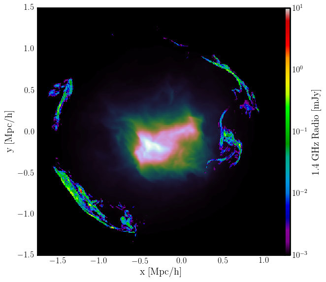
Figure 1.— Simulated X-ray and radio emission. The X-ray in the central regions shows a dynamic range of 100. The radio emission is calculated by placing the simulated cluster at $100Mpc/h$, and masked to show a dynamic range of $10^{4}$.

3. Radio Relic Properties

In this section we describe the general properties of the simulated galaxy cluster. We begin by comparing the morphological similarities between our simulated cluster and several observed clusters. We then move on to describe the other gas properties in an effort to constrain the properties of the radio-emitting plasma. Finally, we will look at the time evolution of these quantities in order to understand their coupling during the merger process.

3.1. Simulated Radio & X-ray

We begin by comparing the radio and X-ray emission from our simulation with the radio relics present in A3376 (see Figure 1a. in Bagchi et al. (2006)) and CIZA J2242.8+5301 (see Figure 1 in van Weeren et al. (2010)). In this work we calculate the X-ray emission using Cloudy to integrate the emission from $0.5-12~{}\mathrm{keV}$ assuming a metallicity of $Z/Z_{solar}=0.3$. The resulting $1.4~{}\mathrm{GHz}$ radio and $0.5-12~{}\mathrm{keV}$ X-ray emission is overlaid in Figure 1. The X-ray is shown in color with a dynamic range of $100$. The radio flux is calculated by placing the simulated cluster at a distance of $100Mpc/h$. We then mask the radio emission such that $10^{-3}-10^{1}~{}\mathrm{mJy}$ is visible. The total integrated flux for the left and right relics are $9.67\times 10^{24}$ and $3.11\times 10^{24}W/Hz$ at $1.4GHz$, which is similar to many of the observed single and double radio relics (Feretti et al., 2012).

There are a few specific details that we highlight here due to their similarities to many observed radio relics. First, we note that this appears as a double radio relic. These are relatively rare compared to their single-sided counterparts. This snapshot is following a major merger roughly $300~{}\mathrm{Myr}$ after core passage. The primary cluster is moving to the lower-left, with the secondary moving primarily to the right. After core passage, a merger shock develops, moving both to the lower left and upper right, and as will be seen in later figures, aligns with strong jumps in temperature and density. The two relic features are aligned with the direction of the merger as well as the shape of the X-ray emission. This alignment of the X-ray morphology and radio emission is characteristic of double radio relics (see Skillman et al. (2011)), as well as many single relics (e.g. van Weeren et al., 2011b; Bonafede et al., 2012).

The second key feature to this simulated double relic is the apparent aspect ratio of the radio emission. The length of the left relic (if we connect the two pieces that are separated by a short distance) is more than $2~{}\mathrm{Mpc/h}$, while the right-moving relic is $1.5-2.0~{}\mathrm{Mpc/h}$. While these relics are quite elongated, they are very thin. In many regions it is at most $100-200~{}\mathrm{kpc/h}$ wide, even in projection. We note here, however, that this width is most likely underestimated since we are not tracking the aged populations of electrons that would exist for some amount of time behind the shock front.

Comparing to A3376 (Bagchi et al., 2006), we see many striking resemblances, including the complex morphology of the Eastern portion of the relic as well as the ring-like structure to the outline of the radio emission. This, at the very least, suggests that the radio-emitting electrons are indeed related to the shock structures formed in merging galaxy clusters. We see a similar structure in CIZA J2242.8+5301 (van Weeren et al., 2010), where the elongation of the X-ray emission points in the direction of the merger, aligning with the double radio relic. We also note the resemblance here with our simulation in terms of the very thin region of radio emission along the relic. This suggests that the cooling times of the relativistic electrons must be short.

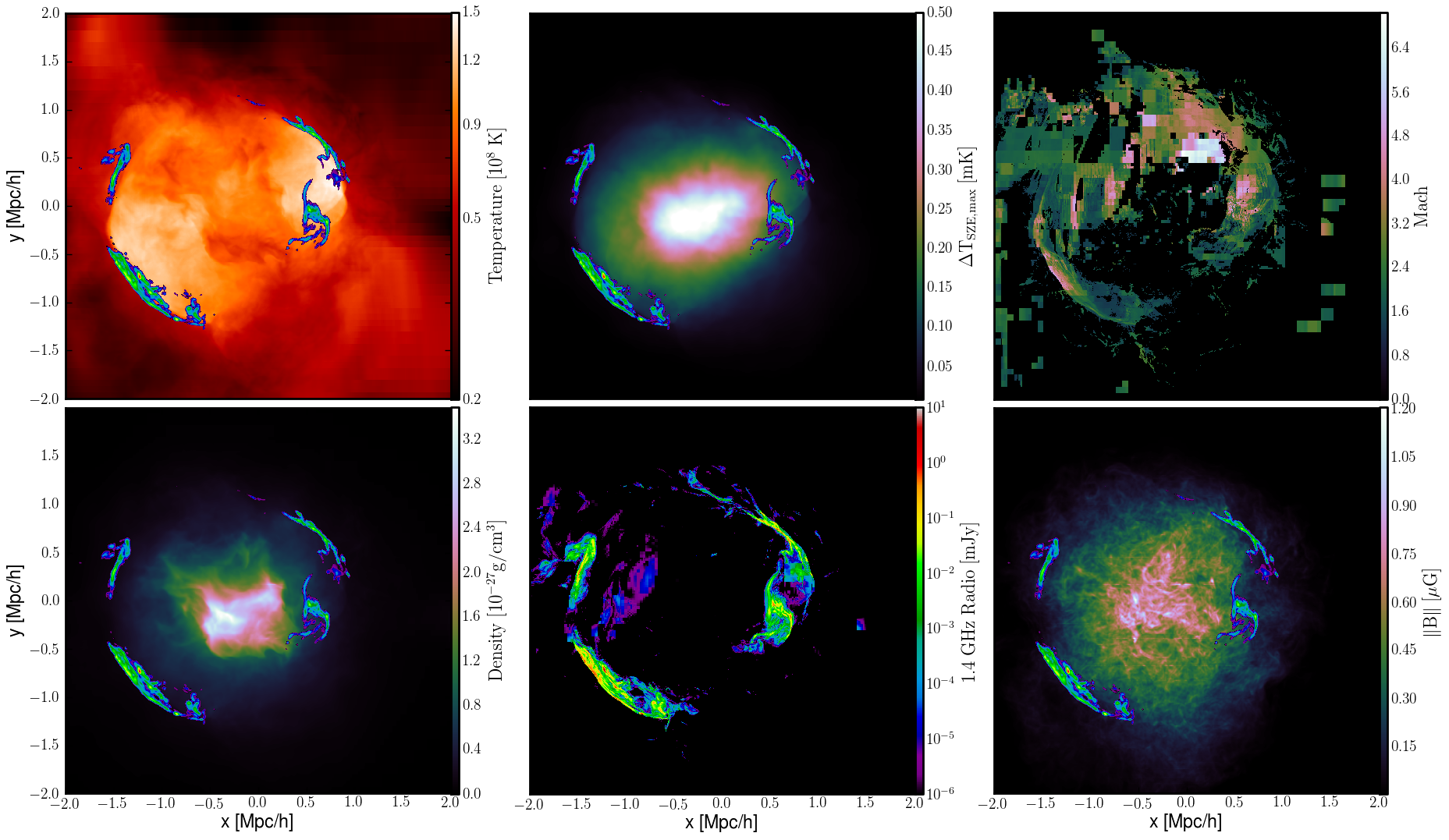
Figure 2.— Projections of gas quantities. Upper left: Temperature, weighted by density. Upper middle: Sunyaev-Zel’dovich Compton-y value converted to the maximum temperature decrement. Upper right: Mach number,weighted by radio emission. Lower left: Density, weighted by density. Lower middle: Integrated radio emissivity. Lower right: Magnetic field strength, weighted by density. Radio emission is overplotted on all panels except the Mach number, and is masked to show between $10^{-3}-10~{}\mathrm{mJy}$. Radio emission assumes cluster is at a distance of $100~{}\mathrm{Mpc/h}$.

Figure 2 shows the fundamental quantities such as density, temperature, Mach number, and magnetic field strength, along with observable quantities such as the 1.4 GHz radio and temperature fluctuations in the CMB due to the thermal Sunyaev-Zel’dovich effect. The radio flux assumes a distance to the simulated cluster of $100~{}\mathrm{Mpc/h}$. Each panel shows the same field-of-view and depth of $4.0~{}\mathrm{Mpc/h}$ at z=0. In all panels except for the radio and Mach number maps, we have overplotted the radio emission to help guide the reader’s eye in determining the location of the emission relative to the underlying plasma. The top left panel shows the density-weighted temperature. Here the correlation between the radio emission and the temperature structure is very strong, as the outward moving shocks are heating the gas to several $\times 10^{8}\mathrm{K}$. Note that the sharp edges in the temperature structure, as well as the maximum in the temperature distribution, occurs $1.5-2\mathrm{Mpc/h}$ away from the center of the cluster. This highlights the unrelaxed nature of this merging cluster.

The bottom-left panel shows the density-weighted density, and has a similar structure to the X-ray image shown in Figure 1, as is expected since the X-ray emission is a strong function of gas density. We note that unlike the temperature, the density is strongly peaked towards the center of the cluster, though the unrelaxed nature is evident by the elongation along the merger axis. The top-right panel shows the kinetic energy flux-weighted Mach number. In addition, we masked out all pixels that contributed $<10^{-10}$ of the peak radio emission. This was done to eliminate some of the shocks along the line of sight that are external to the cluster. The bottom-right panel shows a projection of the absolute magnitude of the magnetic field, weighted by density. Here we weight by density since in many regions there is no relic emission,which would lead to difficult-to-interpret values in the those regions. Notice that the magnetic field also peaks in the center of the cluster around $1~{}\mathrm{\mu G}$. There appears to be a drop in field strength outside the radio relics. This makes sense because the merger shock is just reaching those regions, and then compresses the field behind the shock.

We now use these four quantities to produce the images in the middle bottom column. First, the middle-bottom image shows the radio emission calculated as outlined in Section 2.2. Notice that as expected, the radio emission traces the regions that combine all four of the quantities in the left and right columns. This snapshot of the cluster properties suggests that radio emission requires a combination of dense, hot, magnetically threaded gas in the presence of moderately strong shocks. There are regions in the Mach panel of shocks in the $\mathcal{M}=5-7$ range that only contribute a small amount of radio emission. This region, which can be seen by rotating the viewpoint (not shown in this presentation), happens to lie outside the cluster a bit further where the magnetic field, temperature, and density have dropped considerably. We also notice that the strongest regions of radio emission correspond to Mach numbers in the $3-5$ range with temperatures above $10^{8}K$, similar to findings in Skillman et al. (2011).

Finally, in the top-middle panel, we have overlaid the radio emission on top of the thermal Sunyaev Zel’dovich effect (tSZE). We have taken out the frequency dependence in the $f(x)$ function, and multiplied the tSZE Compton y-parameter by the temperature of the CMB in order to get units of $\mathrm{mK}$. Finally we multiply by $2.0$, the maximum of $f(x)$, to get the maximum decrement value. Notice the very strong correlation with the jump in tSZE and the presence of radio emission. Also note that this image is shown in linear-scale, and the dynamic range in this image is $<20$. This has interesting implications for ongoing and future high-resolution tSZE measurements with MUSTANG (Mroczkowski et al., 2011). CARMA (Plagge et al., 2012), and CCAT (Radford et al., 2009). Since the tSZE is sensitive to the integral of the pressure along the line of sight, it may be preferable to X-ray studies of galaxy cluster shocks because of it’s linear dependence on density and temperature instead of a roughly quadratic dependence on density and sub-linear dependence on temperature. This also minimizes the effects of gas clumping and increases sensitivity to low density gas. This advantage is amplified in the outer regions of galaxy clusters where many of these radio relic shocks are located.

3.2. Density & Magnetic Field Strength Relationship

In the next two sections we will describe the physical properties of the radio emitting plasma in order to compare to what has been found observationally. In the following analysis, we use the inner-most nested refined region of the simulation $(32~{}\mathrm{Mpc/h})^{3}$ and ignore the lower-resolution regions in the remainder of the simulation. We choose to study this entire sub-volume instead of regions defined by the virial radius because the cluster is undergoing a major merger. Within this region, we bin various quantities such as radio emission, density, temperature, and magnetic field.

Before we discuss the radio emission, we first describe the structure of the magnetic field. In Figure 3, we show the average magnetic field strength as a function of density, along with the $1-\sigma$ standard deviation where the average is weighted by density. This is similar to plots found in Dubois & Teyssier (2008), though in their study they also followed gas cooling. Contrary to what has been assumed in prior studies such as Hoeft et al. (2008); Skillman et al. (2011), we find that the magnetic field does not scale with $\rho^{2/3}$, but instead with $\rho$ at low density and has an inner core with roughly flat magnetic field at high density. This was discussed previously in Xu et al. (2011), casting doubt on assumptions of any tight relationship between density and magnetic field strength. This suggests that the manner in which we inject the magnetic fields may ultimately determine quantities such as the total radio luminosity. Future work should explore the effects of varying the magnetic field injection mechanism. For example, we may expect a shallower slope and more evenly distributed field strength if we inject magnetic fields from multiple sources instead of seeding each cluster with a single source.

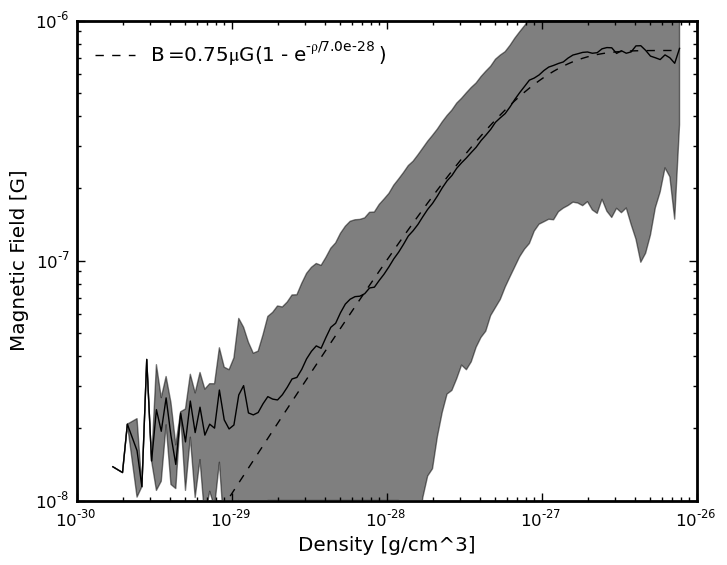
Figure 3.— Average magnetic field strength as a function of density, where each cell is weighted by the density, with the shaded area denoting the standard deviation. For reference, we show an analytic function that is linear with $\rho$ at low density and flattens at high density.

Because of the steep drop in magnetic field strength at low densities, we expect that the radio emission will similarly decrease towards the outskirts of the cluster. Additionally, because the field strength flattens out at high density, we expect to see radio emission that is not necessarily biased to the highest density regions near the center of the cluster.

3.3. Kinetic Energy & Radio Emission Distributions

The next quantity we will use to describe the gas properties of the cluster are the kinetic energy flux through shocks and the radio emission based on the Hoeft & Brüggen (2007) model. We find it useful to show both of these quantities with respect to density, Mach number, magnetic field strength, and temperature in order to characterize the gas that is most responsible for the conversion of kinetic energy to cosmic-ray electrons. For this particular study, we choose to show both kinetic energy flux as well as the radio emission. As seen in Section 2.2, the radio emission is a complex function of many quantities, and it is difficult to disentangle each variable. The kinetic energy flux, however, is a much simpler quantity, relying only on the density, velocity, and temperature of the incoming gas: $F_{KE}=0.5\rho v^{2}\mathcal{M}c_{s}$.

The top left panel of 4 shows the kinetic energy flux through shocks as a function of Mach number on the x-axis, and the magnetic field strength on the y-axis. Note that all un-shocked cells in the volume are ignored. For each bin, we calculate the kinetic energy, and normalize by the maximum value from all the bins. This distribution is shown in logarithmic space, as only a small number regions dominate the kinetic energy flux. In this figure there appears to be 3 primary populations of gas that contribute to the kinetic energy flux. The first is a very low Mach number ($\mathcal{M}<1.5$), high-magnetic field, region of the simulation, which corresponds to the turbulent flow in the center of the galaxy cluster. This slightly supersonic flow processes a large amount of kinetic energy because of the high density and high temperature (and therefore sound speed), even though the Mach numbers are low. On the upper end of the shock Mach number scale, there are shocks around a Mach number of 6-8 with a magnetic field strength below $0.01~{}\mathrm{\mu G}$. These, as we will discuss later, are associated with shocks onto filaments.

The third population in the kinetic energy flux is at Mach numbers between $3-5$ with a magnetic field strength of between $0.1-1.0~{}\mathrm{\mu G}$. These are the two primary merger shocks, which we will see are the main source of the radio emission. Note that this is not a single or even pair of distinct Mach numbers, meaning that observationally, a given merger shock should not be characterized by a single Mach number. If the properties of shock-accelerated electrons are strongly dependent on the Mach number, ascribing a single Mach number may lead to inconsistencies in the fitting to the observed radio emission.

The lower-left panel shows the same quantity in color, but now decomposed into density and temperature bins. Here we get a different view of the same result. In this panel there are several knot-like regions in phase space, which likely correspond to each of the primary shocks in our cluster. However, in this case we see that there are 3-4 regions. There is a very low-density, $10^{6}-10^{7}~{}\mathrm{K}$ region that likely corresponds to outer accretion shocks onto the filaments. The other regions of high kinetic energy at more intermediate densities correspond to each of the primary merger shocks in the cluster. The large clump at very high temperatures and a density of roughly $10^{-28}~{}\mathrm{g/cm^{3}}$ corresponds to the left-moving shock at $\mathcal{M}\sim 4$. This will become even more apparent when we examine the right panels of this figure. The primary results of this study of the kinetic energy flux agrees well with prior studies of the distribution of kinetic energy flux in shocks (Ryu et al., 2003; Pfrommer et al., 2006; Skillman et al., 2008; Vazza et al., 2009, 2011). However, this is the first time they have also been correlated with the magnetic field distribution.

Now we contrast the distributions in kinetic energy flux with the radio emission. In the right panels of Figure 4, we use the color scale to signify the total radio emission. In the top right panel, we again show radio emission as a function of Mach number and magnetic field strength. Here we see that of the three features present in the kinetic energy flux, only one remains in the radio emission. This corresponds to the regions where the three ingredients needed to create radio emission are all present. The Mach number is above the threshold for accelerating high energy electrons, the gas is dense enough, and the magnetic field strength is high enough. We note that the falloff at low Mach numbers is due to the functional form of $\Psi(\mathcal{M})$ from Equation 1. For this simulation, we find that the majority of the radio emission in this cluster comes from shocks with Mach numbers of $3.0-6.0$ and magnetic field strengths of $0.1-1.0~{}\mathrm{\mu G}$.

The same general conclusions are found from the lower right panel. We see that, instead of a fairly broad distribution in kinetic energy flux across densities and temperatures, the radio emission is confined to regions of relatively high densities and temperatures near $10^{8}~{}\mathrm{K}$. By combining this with the upper-right panel, we have determined the exact makeup of the gas responsible for the synchrotron radiating electrons in radio relics.

It is important to note that the magnetic field in our simulation does not reach the levels calculated from observations of several radio relics (Clarke et al., 2001; Clarke, 2004; van Weeren et al., 2010). This suggests that the magnetic field injection mechanism used in this study may not correspond to how it occurs in observed galaxy clusters. Alternatively, amplification of pre-existing fields prior to AGN injection, primordial magnetic fields, and several other processes such as turbulent dynamo (Iapichino & Brüggen, 2012) in the post-shock region and the streaming instability (e.g. Achterberg & Wiersma, 2007) may lead to higher magnetic field values, all of which could be investigated in future work. Finally, observations should be re-examined to determine if a lower value of magnetic field is possible, such as what has recently been found in Carretti et al. (2012).

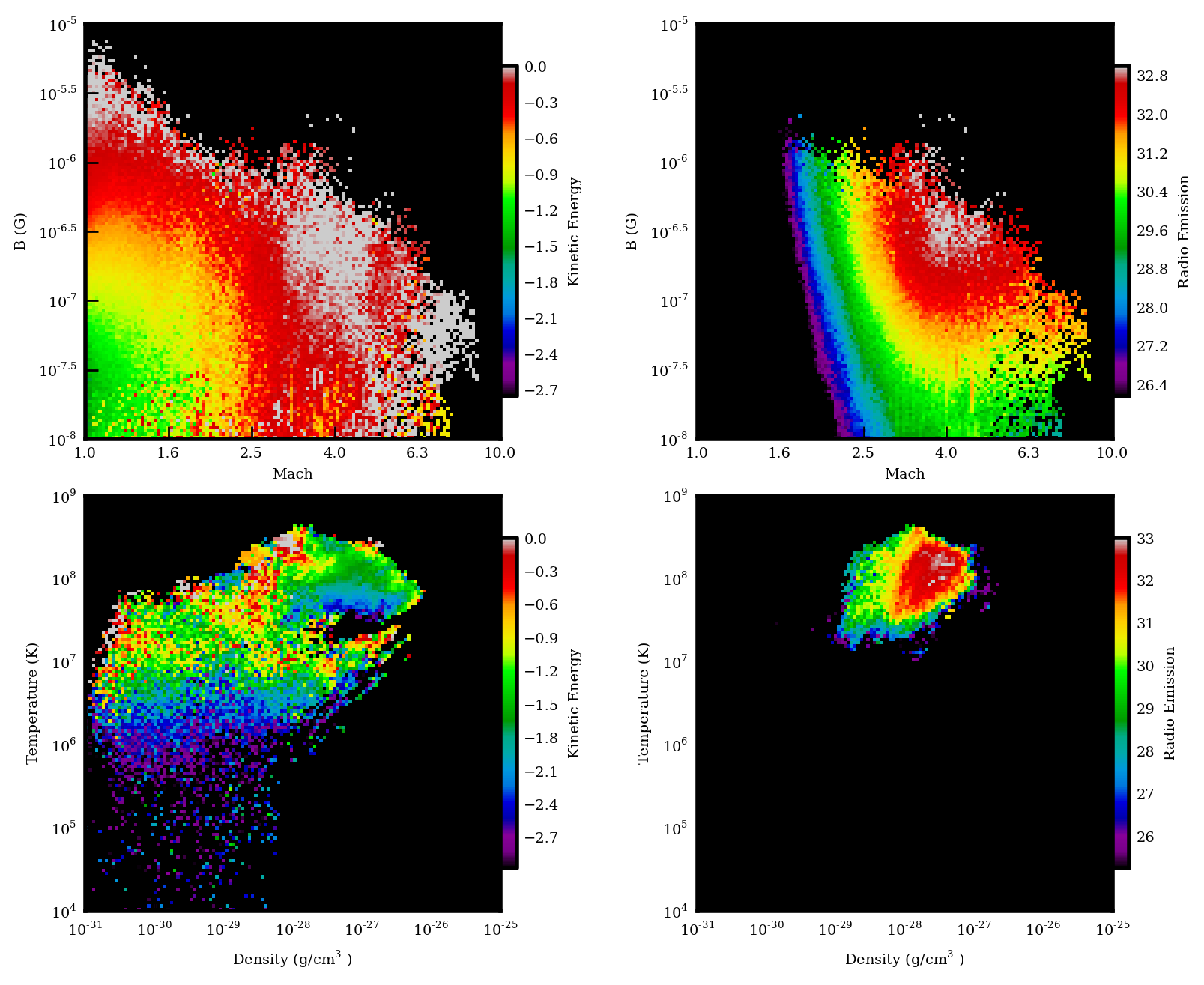
Figure 4.— Phase plots of gas properties indicating the location of the kinetic energy flux and radio emission at shock fronts. The left plots show the kinetic energy distribution, while the right plots follow the radio emissivity. The top panels show the distributions as a function of magnetic field strength on the y-axis, and Mach number on the x-axis. The lower panels show them as a function of temperature on the y-axis, and density on the x-axis.

3.4. Merger Evolution

Observationally, we are limited to a single snapshot in time, from which we must deduce the prior and future evolution of a given galaxy cluster. Fortunately this is not the case for simulations. In this section we describe in detail the evolution of the gas properties throughout the history of the clusters we are modeling. Figure 5 shows the evolution of bulk properties in the nested region of the simulation from redshift $z=2.95$ to $z=0.0$. There are five quantities shown here.

1. Density: Average density, weighted by density.

2. Temperature: Average temperature, weighted by density.

3. Magnetic Field: Average magnetic field strength, weighted by density.

4. Radio: Total 1.4 GHz Radio Emission

5. Xray: Total 0.5-12 keV X-ray luminosity

In each case we select the inner-nested region of the simulation, and use WeightedAverageQuantity or TotalQuantity “derived quantities”. Each of these averages and totals are then saved for future analysis. In the case of Figure 5, we normalize each of the quantities by their maximum value in order to fit them all on the same scale. In the case of the X-ray and radio luminosity, the emission is calculated using the blueshifted frequencies as these would be redshifted into the observer’s frame to be at the correct values ($0.5-12\mathrm{keV}$ and $1.4\mathrm{GHz}$ for X-ray and radio, respectively).

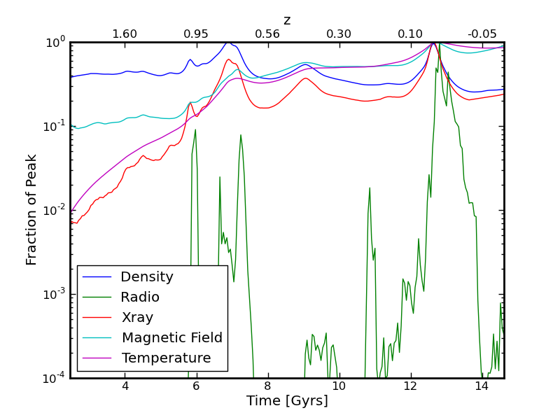
Figure 5.— Time evolution of integrated gas properties in the volume surrounding the structures of interest. For density, temperature, and magnetic field, we calculate a weighted average, using density as the weight. For radio and X-ray values, we calculate the total emission within the innermost nested region of the simulation. Note the simulation was run beyond $z=0$ to allow the merger to finish.

We find a very interesting correlation with all of the fundamental and derived quantities. First, it is clear that there was not only the late-time merger near $z=0$, but also earlier merger evolution near $z=1$. First, we see that the density and temperature both start to rise $0.2-0.5\mathrm{Gyr}$ before the radio emission spikes. Analogously, the magnetic field and X-ray luminosity also follow this slow rise to a peak. Near the peak, the radio emission jumps up several orders of magnitude. This corresponds to the formation of the shock front that then moves outwards from the cluster center towards the outskirts of the cluster. After the core passage, the density and temperature returns to a lower but elevated level with respect to the pre-merger values.

This suggests that the radio emission lags the merger event by a few $\times 10^{8}$ years while the shock is setting up and expanding into the intracluster medium. It again highlights the dependence on not only the local characteristics of the emitting plasma, but also the shock surface area. Another key point is that the short timescales over which the radio luminosity varies implies that for a given mass or X-ray luminosity, there may be very large scatter in the radio luminosity. Overall, the radio emission is only above $10\%$ of its peak value for $\sim 0.5~{}\mathrm{Gyr}$. This could help explain the observed lack of radio emission from clusters with obvious mergers such as Abell 2146 (Russell et al., 2011). One caveat to this result is that we do not follow the electrons as they cool. However, because the cooling timescale,

$$\tau\approx 2\times 10^{12}\gamma^{-1}((1+z)^{4}+(B/3.3\mu G)^{2})^{-1}~{}\mathrm{years}$$ (14)

for these electrons with $\gamma\sim 1000-5000$ is short (Ferrari et al., 2008), this additional time has little effect. Therefore the characteristics of this time evolution should not change substantially with a proper treatment of the aging electron population.

4. Observational Implications

In this section we set out to provide a theoretical perspective on the analysis of observed radio relics. In particular, we comment on some of the assumptions that are often employed, and in several cases point out how these may be dubious. We begin by examining how the viewing angle of a radio relic can impact its interpretation. We expand on this point in the context of spectral index analysis, where not only does viewpoint play a role, but small-scale fluctuations in the shock properties can lead to observational signatures that mimic an aging population of cosmic ray electrons. Finally, we point out the limitations of our models; specifically, we must include aging populations of electrons in future calculations in order to capture accurate polarization fraction and direction.

4.1. Viewpoint

Observationally, we are limited to a single viewing angle for each object. Unfortunately, because radio relic emission is not spherically symmetric, there will be a viewing angle-dependent emission strength and morphology. In this section we set out to demonstrate this fact and how it can affect our interpretation of radio emitting regions in galaxy clusters. We begin by taking our original viewpoint and rotate the viewing angle by 180 degrees over 18 frames. The result is shown in Figure 6, where radio emission is projected along each viewing angle.

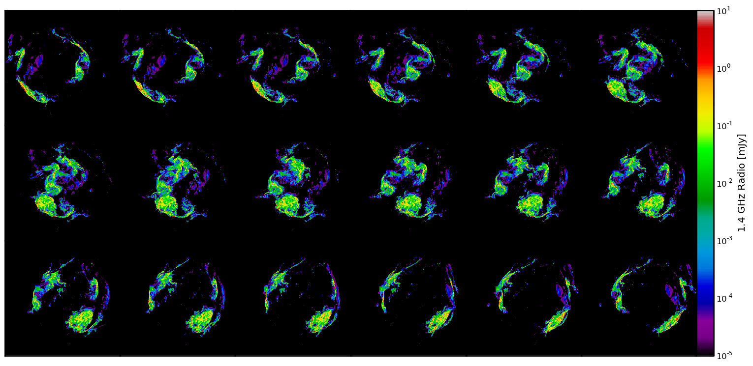
Figure 6.— 180 degree rotation of radio emission. Flux computed by assuming a distance of 100 Mpc. Each panel is rotated by 10 degrees from the previous, moving left to right, top to bottom. Note that this panel of images acts as a autostereogram, and can be used to see the 3D structure of the radio emission. For an animation, see http://www.youtube.com/watch?v=WNez-h3uOPA

What can be seen from Figure 6 is that, while for some orientations the radio emission forms an obvious “double relic” configuration, other orientations yield what seems to be a single, more diffuse, object. However, given a single frame, it would be difficult to determine the true structure of the emission. In fact, this may lead to a misinterpretation of the radio emission to be that of radio halo origin. We will expand upon this line of reasoning in Section 4.2. There are several other things to note here in the rotation of the radio emission. We see that in some orientations (see top row, 5th & 6th columns), we reproduce morphologies that include two outer relics, with one of the relics ending up between the two, close to the center of the cluster. This is very similar to observed clusters such as $\mathrm{MACS\ J1752.0+4440}$ (van Weeren et al., 2012), $\mathrm{CIZAJ2242.8+5301}$ (van Weeren et al., 2011d), and $\mathrm{MACS\ J0717.5+3745}$ (van Weeren et al., 2009). It may be possible that the emission in these clusters be not of radio halo origin, but simply radio relic emission viewed coincident with the cluster center. Similar work has been done with hydrodynamic simulations of galaxy clusters and viewing them along the coordinate axes in Vazza et al. (2012), where they found that the low emissivity due to the small size along the line of sight may explain the lack of central radio relics.

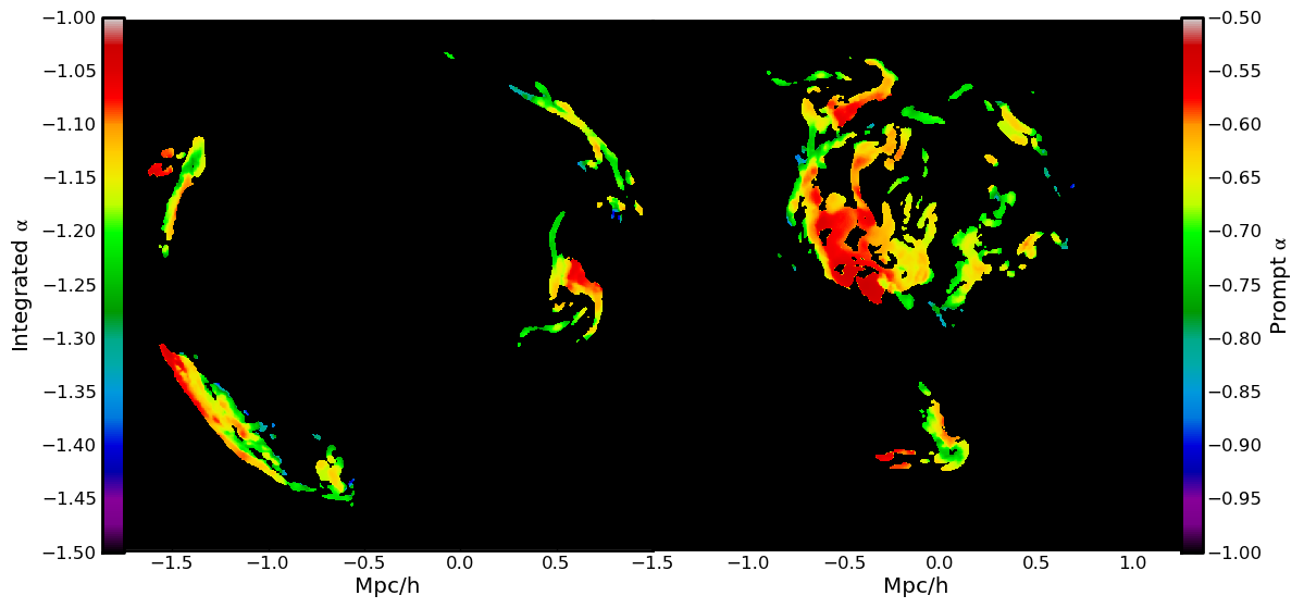
Figure 7.— Spectral index of simulated radio relic emission. The left portion of the image shows the “edge-on” view, whereas the right shows the “face-on” view. Both views are on the same scale. The left colorbar shows the mapping of color to the integrated spectral index including particle aging. The right colorbar shows the mapping of color to the prompt spectral index. Both colorbars apply to both views, providing a rough estimate of the uncertainty in our models of the spectral index.

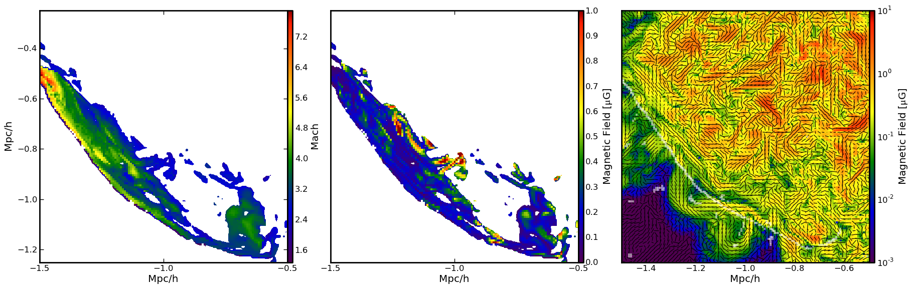
Figure 8.— A zoom in of the lower left radio relic. The left two panels show radio emission-weighted projections of the Mach number (left), and magnetic field strength (middle). The right panel shows a slice of the magnetic field strength, with black lines indicating the local magnetic field direction in the plane of the slice and the white overlay show the location of cells identified to be shocks.

4.2. Spectral Index

Observationally, the spectral index of cluster radio relics is measured by comparing the emission at several different observed frequencies. In our work, we calculate the spectral index by first calculating the radio emission at two frequencies (here we use 1.4 GHz and 330 MHz). After smoothing by a Gaussian with a full-width half maximum size of 4 pixels, we then use these two maps to calculate the spectral index, similar to what would be done observationally. Because we use the Hoeft & Brüggen (2007) model, we will recover a spectral index from comparing these two maps that is equal to the cumulative spectral index due to the emission from electrons over their entire lifetime. This is steeper than the spectral index that would be predicted from the prompt emission from a shock front, which is related by $\alpha_{prompt}=(1-2\alpha_{integrated})/2$.

In reality, what is thought to happen is the leading edge of the shock front should accelerate electrons to $\alpha_{prompt}$. As the radio emitting electrons move downstream from the shock they cool and the spectrum steepens. Qualitatively, we would expect that “edge-on” observations should produce values near $\alpha_{prompt}$, whereas a “face-on” view would be sensitive to the entire lifetime of the electrons, and therefore be closer to $\alpha_{integrated}$.

Spectral steepening is found to happen in several observed clusters (van Weeren et al., 2011a) and measuring the steepening of the electrons as they progress away from the shock can help constrain the local magnetic field, as was done in van Weeren et al. (2011a). However, the assumption in these calculations is that the spectral steepening is due entirely to the aging of the electrons. However, we see similar steepening even though we do not include the spectral aging of the electrons as they advect downstream! These variations are entirely due to a varying magnetic field and shock strength in a non-uniform medium. The spectral indices of the prompt and integrated spectra are shown in Figure 7, and the fluctuations in the underlying fields for the lower-left “edge-on” relic are shown in the right panel of Figure 8.

In Figure 7, we see that the “edge-on” view shows a spectral steepening whereas the “face-on” view shows the spatially variant spectral shape due to the shock properties. For completeness we have mapped the colormap of both viewing angles to both the prompt and integrated spectral indices. The same qualitative behavior is seen with both calculations. These fluctuations are explained in Figure 8, where we see that the radio emission-weighted Mach number can vary between $2-8$, and the magnetic field can vary from $0.1-1\mu G$. Therefore we warn that extrapolating from the measured spectral steepening to calculate gas properties should be done with care, as projection effects and spatial variation of the gas properties are important. It may be insufficient to prescribe a single Mach number or magnetic field to a given radio relic.

4.3. Polarization Fraction & Direction

Using our newly developed method, we have created radio polarization fraction and direction maps for our galaxy cluster from two viewing positions. The first gives an “edge-on“ view of the radio relic, whereas the second is aligned such that the relics are viewed “face-on.” We will examine, in detail, the polarization signatures of the “edge-on,” and then describe the differences in the “face-on” view.

In Figure 9, we show the linear polarization fraction and direction of $1.4\mathrm{GHz}$ radio emission. Lines denote the local linear polarization direction, the length of which corresponds to the polarization fraction. For clarity, the polarization fraction is also shown in color. The polarization fraction is calculated using

$$f_{p}=\frac{\sqrt{I_{x}^{2}+I_{y}^{2}}}{I}$$ (15)

In this case we use a $512\times 512$ pixel image plane to project through a cube of length $4~{}\mathrm{Mpc/h}$ on a side. At full resolution $(7.8\mathrm{kpc/h})$, we see that the polarization fraction reaches a maximum of $\sim 75\%$, and that the polarization direction is correlated along the relic, primarily perpendicular to the shock. This is very similar to what is found observationally in CIZA J2242.8+5301 (van Weeren et al., 2011a). The authors find strong (50-75%) polarization at what is presumed to be the leading edge of the shock. Additionally, they find that the polarization direction is fairly constant over the length of the relic. We do, however, see greater variation in the polarization fraction and direction both across and along the relic. These fluctuations in our simulation may suggest that there are additional physical processes which lead to a more ordered field. In order to investigate the small scale fluctuations in the polarization direction, we examined a slice of the magnetic field strength and direction through this relic. This is shown in Figure 8. What we found is that while the shock (overlaid in white) cuts through regions which have fairly strong variations in the magnetic field direction, the region “behind” the shock has a magnetic field that is compressed along the shock propagation direction. Therefore, it may be possible that if we were to follow the evolution of the cooling electrons as they moved downstream across the shock, the magnetic field that they reside in may become more ordered parallel to the shock, leading to a longer coherence length as more constant polarization direction. Therefore we would expect that in future work when we examine the emission from an evolving population of cosmic rays, we should see even better agreement with observations of polarization direction.

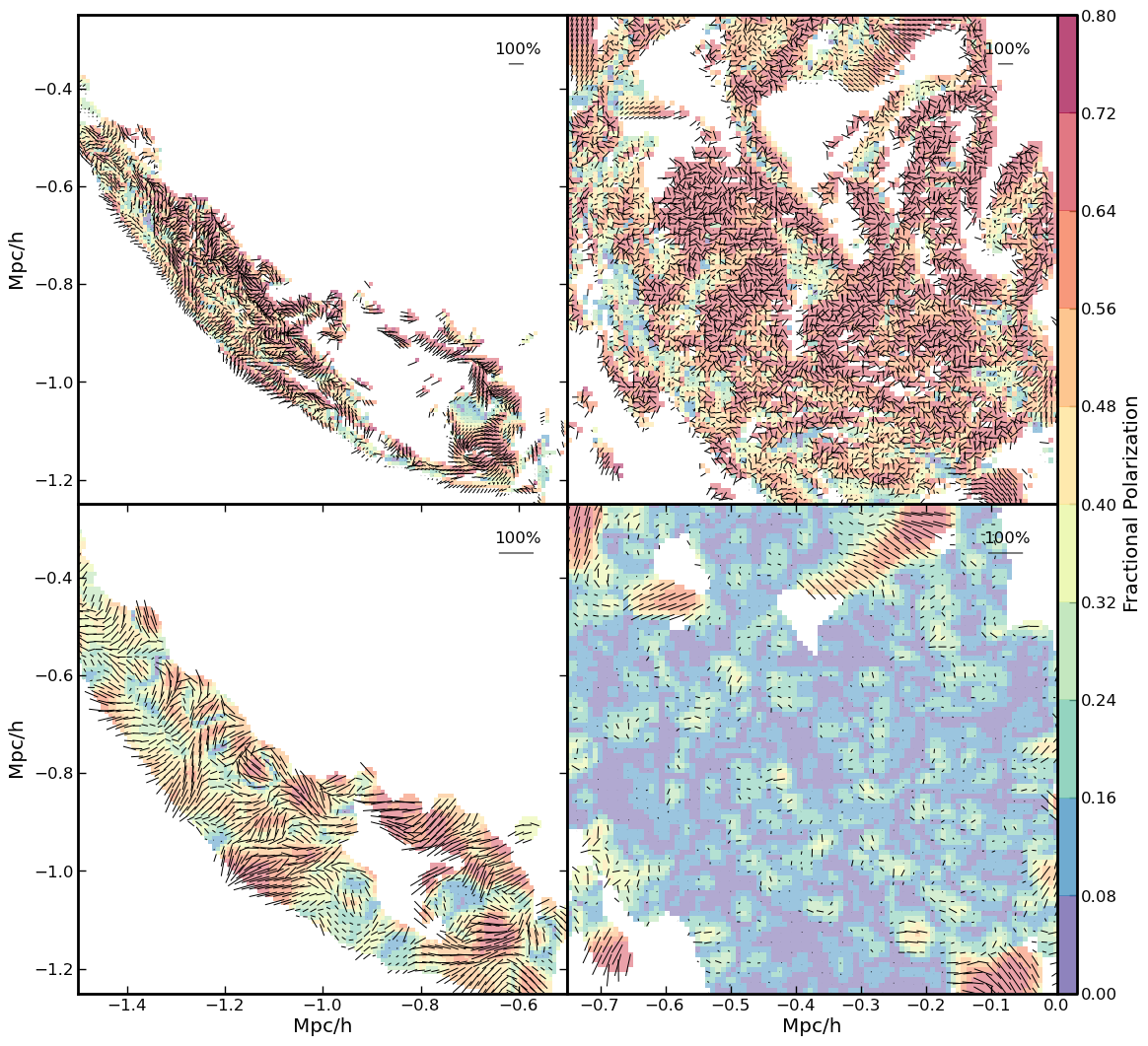
Figure 9.— Polarization fraction and direction. In each panel, the polarization direction is denoted by the black quivers, while the polarization fraction is represented by both the color scale as well as quiver length. The top panel shows the relic at full resolution $(7.8\mathrm{kpc/h})$, while the lower panels show the same view at 4 times worse resolution. At $z=0.2$, the redshift of CIZA J2242.8+5301, this corresponds to angular resolutions of $3.36^{\prime\prime}$ and $13.44^{\prime\prime}$, respectively. The left panels show the polarization for the “edge-on” (top) while the right shows the “face-on” view.

In the top-right panel of Figure 9, we show the same polarization map, but this time for when the relic is viewed “face-on”. We again see a very high polarization fraction. However, this time the polarization direction is significantly less coherent. This is due to the magnetic field not being modified as strongly in the plane of the shock as it is perpendicular to the shock. Therefore the turbulent structure is preserved in the image plane and the polarization vectors are not preferentially modified.

However, the behavior of the polarization fraction and direction drastically changes if we then apply a guassian kernel with a size of 4 pixels. In the “edge-on” view, the polarization fraction and direction is fairly well preserved. The fraction only drops to between $30-65\%$ and the direction is still fairly correlated across the relic. In contrast, for the “face-on” view the polarization has dropped to between $0-15\%$ in most regions. This is a classic example of beam depolarization. Because the polarization direction is highly disordered, smoothing the image drastically reduces the overall polarization.

Currently our simulations do not exhibit as much of a constant polarization as that found in observations of clusters such as CIZA J2242.8+5301, where the polarization direction is constant over Mpc-scale distances. There are several possible explanations. Because we are not tracking the electron distribution as it cools behind the shock, we may be missing the emission from the more ordered field line regions behind the shock. Simulations capable of tracking these electrons are therefore needed to explore that possibility, and will be addressed in future work. If doing so is still incapable of producing Mpc-scale ordered polarization maps, it may suggest that the injection mechanism or magnetic field evolution is different than what we have simulated.

5. Discussion & Future Directions

We have carried out high resolution MHD AMR cosmological simulations using an accurate shock finding algorithm with a radio emission model for shock-accelerated electrons to examine the properties of radio relics in galaxy clusters. We summarize the physical conditions of the cluster, and several of the warnings for the interpretations of observed radio features:

• Cosmological initial conditions lead naturally to the formation of giant radio relics whose properties are very similar to observed relics. This is a natural result of the process of mergers that create galaxy clusters, where the magnetized intracluster medium is subject to a series of strong, large-area shocks.

• We find that the radio emission in our simulated clusters is strongest in plasma that has $0.1-1.0~{}\mathrm{\mu G}$ magnetic fields with a shock Mach number between $3-6$, with densities near $10^{-28}~{}\mathrm{g/cm^{3}}$ and temperatures of $10^{8}~{}\mathrm{K}$.

• If the shock acceleration efficiency for electrons is higher than assumed at low Mach numbers, a large reservoir of kinetic energy becomes available in hot $(10^{7}~{}\mathrm{K})$ gas at both lower and higher densities than what is currently producing emission in our simulations.

• We find a magnetic field distribution that does not follow the often assumed $B\propto\rho^{2/3}$ relation. Instead, it follows $B\propto\rho$ at low densities, and flattens out to $\mathrm{sub-\mu G}$ levels above densities of $10^{-27}\mathrm{g/cm^{3}}$.

• Warning: Without a model of spectral aging of electrons, we still recover a spectral index gradient, indicating that observed gradients should not necessarily be interpreted as the spectral aging of electrons. It may simply be due to the projection of a curved shock front with varying Mach number.

• Warning: From the time evolution of our simulated galaxy cluster, it is clear that only a small portion of its lifetime may be spent in a regime where it is bright in the radio wavelengths. This may explain the apparent lack of observed radio emission in some massive galaxy clusters with early or late phase merger.

• Warning: The viewing angle of a given galaxy cluster may have significant impact on the classification of its radio emission. Double radio relics viewed at some orientations are difficult to differentiate from radio halo emission.

• Warning: Future simulations of galaxy cluster radio relics must follow the temporal evolution of the electron population in order to reproduce valid polarization results, as the downstream conditions from the shock may include more ordered magnetic fields, leading to different polarization maps than when the emission is assumed to come only from the shock center.

Many of these warnings apply both to observational and theoretical studies, and the classification and analysis of radio relics in all contexts must be done with care to avoid confusion with radio halo emission. There are several advancements that can be made theoretically. We are in the process of developing and testing the numerical framework necessary to follow the cosmic ray electron and proton populations, using a method similar to Miniati (2001) and Jones & Kang (2005). Doing so will allow us to probe the spectral distribution of these non-thermal populations in the context of high-resolution cosmological simulations. Once this is merged with our ability to produce synthetic emission and polarization maps, we will be able to more directly compare to current observations. Additionally, we do not explicitly include any magnetic field source terms at the shock fronts. Exploring local field generation mechanisms such as the Weibel instability (Weibel, 1959; Fried, 1959) may allow for alternate magnetic field strength and structure behind the shock front from what we present here. Finally, we may need to push to higher resolution studies at the shock fronts to be able to follow the shock-amplification of magnetic fields. Doing so in a cosmological simulation is currently intractable; however, improvements in computational speed and parallelization may allow for future studies.

Observationally we are entering a golden age of radio telescopes with the upgraded Jansky VLA, GMRT, and LOFAR, and are looking forward to the SKA, and possibly a lunar farside radio telescope(Burns & Lazio, 2012; Lazio et al., 2009). These improvements will lead to greater sensitivity and bandwidth, allowing for multifrequency studies of galaxy cluster environments in unprecedented detail. However, only through a coordinated effort between simulations and observations will we be able to fully understand the plasma physics in these cosmic environments.

Appendix A Polarized Emission Integration

In this section we detail the integration methods used to calculate the total and polarized radio emission Faraday rotation. Where possible, we follow the conventions listed in Longair (1994) and Otmianowska-Mazur et al. (2009). As input to the system, we will assume that there is an emissivity, $\epsilon~{}[erg/s/cm^{3}/Hz]$; magnetic field, $\vec{B}~{}[G]$; electron number density $n_{e}~{}[cm^{-3}]$; and viewing angle, $\vec{L}$.

From the viewing angle and magnetic field, we first decompose the magnetic field into components along the line of sight $B_{||}$ and perpendicular to it $B_{\perp}$. We use $\theta$ to represent the angle between the $\vec{L}$ and $\vec{B}$, where we $\theta$ has a range of $0-\pi$.

$$B_{||}=\vec{B}\cdot\vec{L}=|B|cos(\theta)$$ (A1)

$$B_{\perp}=|B|sin(\theta)$$ (A2)

We then further decompose $B_{\perp}$ into components aligned with the east and north vectors in the image plane, here referred to as $B_{x}$ and $B_{y}$. Using $B_{x}$ and $B_{y}$, we then define an angle field, $\chi$,

$$\chi=(tan^{-1}(B_{y}/B_{x})~{}+~{}\pi/4)~{}\%~{}\pi$$ (A3)

where we explicitly cast the $tan^{-1}$ into $[0..\pi]$. $\chi$ represents the local direction of the electric field in the image plane. We then use this value to calculate the fractional polarized emission along the east and north vectors,

$$f_{p}=(s+1)/(s+7/3)$$ (A4)

$$\epsilon_{px}=\epsilon f_{p}|\frac{B_{\perp}}{B}|cos(\chi)$$ (A5)

$$\epsilon_{py}=\epsilon f_{p}|\frac{B_{\perp}}{B}|sin(\chi)$$ (A6)

where $f_{p}$ is the polarization fraction, defined using the spectral index of the relativistic electrons, $s$.

Once these emission terms have been defined, we then integrate through a simulation, accounting for the Faraday rotation,

$$\Delta\psi=2.62\times 10^{-17}n_{e}\lambda^{2}B_{||}dl$$ (A7)

where $\mathrm{dl}$ is in units of cm. All of this is then integrated to calculate the total intensity $I$, and the polarized components $I_{x}$ and $I_{y}$, which is written using the discrete approximation:

$$\left[{\begin{array}[]{cc}I_{i+1}\\ I_{x,i+1}\\ I_{y,i+1}\\ \end{array}}\right]=\left[{\begin{array}[]{ccc}dl&\ 0&\ 0\\ dl\ f_{p}\ (\vec{v_{x}}\cdot\vec{E})&\ cos(\Delta\phi)&\ -sin(\Delta\phi)\\ dl\ f_{p}\ (\vec{v_{y}}\cdot\vec{E})&\ sin(\Delta\phi)&\ cos(\Delta\phi)\\ \end{array}}\right]\left[{\begin{array}[]{cc}\epsilon_{i}\\ I_{x,i}\\ I_{y,i}\\ \end{array}}\right]$$ (A17)

where the index $i$ represents the i’th cell along the line of sight.

As a test of this method, as implemented using yt, we initialize a completely polarized background at the simulation domain boundary, with the polarization angle pointing horizontal in the image plane. To do so, we override the emission, polarization fraction, density, and magnetic field strengths in the simulation presented in this paper. In this case, we set the magnetic field equal to 0 (though for numerical reasons we use a very small number), except for a sphere of with a radius equal to one-quarter of the simulation domain size. Inside this sphere, we allow the magnetic field parallel to the line of sight to be exactly that which will, for rays passing through the center of the sphere towards the “observer”, be enough to rotate the polarization vector by $\pi$. We show the results of this test using $128^{2}$ pixels in Figure 10 for both on-axis $(\vec{L}=(1,0,0))$ and off-axis $(\vec{L}=(1.0,0.3,0.7))$, where we find excellent agreement with the expected behavior. For both viewing angles, the maximum of $f_{p}-1.0\approx 10^{-14}$, and the polarization angle has a fractional error in the center of the image of $1.7\times 10^{-5}$ for on-axis, and $1.3\times 10^{-2}$ for off-axis. Given the coarse nature of the sampling of this image and the likelihood that the center pixel doesn’t exactly traverse the center of the sphere, these should be viewed as upper limits.

As a second test, we initialize two $y-z$ planes of radiation each with electric field vectors that are perpendicular to each other along. For the first plane, we set $B_{x}=B_{z}=0.0$, and $B_{y}=1.0$. The second plane has $B_{x}=By=0.0$ and $B_{z}=1.0$. Each plane has a width equal to $\frac{1}{32}$ of the simulation width, centered at $x=\frac{1}{64}$ and $\frac{63}{64}$ in units of the simulation width. We set the image width equal to $2.0$ and use $256^{2}$ pixels. Finally, we begin by looking from $(-1,0,0)$ towards $(1,0,0)$, centered on $(0.5,0.5,0.5)$, and rotate in the $x-y$ plane. Therefore in all cases plane 2 has a magnetic field that is vertical and plane 1 begins with a horizontal magnetic field but then proceeds to have a component along the line of sight. For this test we disable the Faraday rotation, and examine only the effects of combining two planes of radiation on off-axis lines of sight. We vary the rotation from the original viewpoint to have angles of $\theta=(0,5,15,30,60)$. In Figure 11, we show the fractional polarization as a function of image pixel. In all cases for the portions of the planes that overlap along the line of sight, the calculated polarization fraction is within double precision fractional error of the expected polarization fraction.

All of these capabilities are demonstrated in a public repository, found using the changeset with hash fc3acb747162 here: https://bitbucket.org/samskillman/yt-stokes. Future improvements to this code as well as tighter integration in the primary yt repository is expected, both in performance and usability.

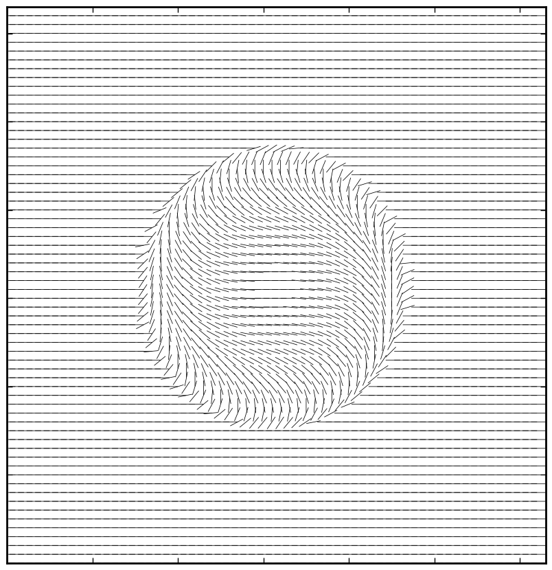
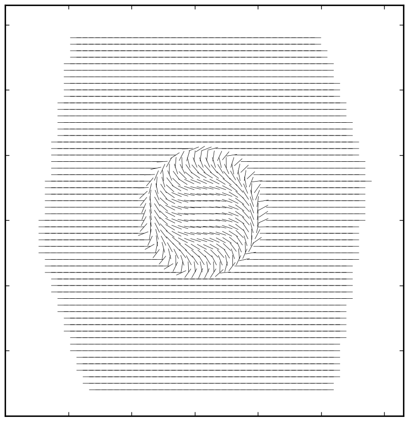
Figure 10.— On and off-axis Faraday rotation test. The left panel shows the on-axis Faraday rotation through a magnetized sphere, with an image width equal to the domain size. The right panel shows the same rotation, but off-axis and with a width of $1.6$ larger than the left, to show the off-axis nature of the domain. The electron number density and magnetic field strength of the sphere are chosen to rotate the polarization angle $\pi$ radians for the rays passing through the center of the sphere.

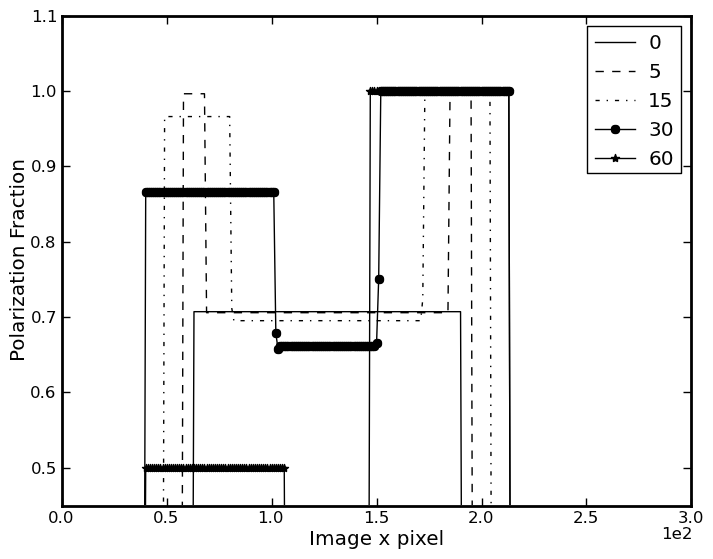
Figure 11.— Dual plane polarization test. The polarization fraction as a function of image pixel across the mid-plane of the image, shown for varying viewing angles that are measured as an offset in the $x-y$ plane from a viewing direction of $\vec{L}=(1,0,0)$.

References

- Achterberg & Wiersma (2007) Achterberg, A. & Wiersma, J. 2007, A&A, 475, 1
- Ackermann et al. (2010) Ackermann, M. et al. 2010, ApJ, 717, L71
- Akamatsu et al. (2012) Akamatsu, H., Takizawa, M., Nakazawa, K., Fukazawa, Y., Ishisaki, Y., & Ohashi, T. 2012, PASJ, 64, 67
- Aleksić et al. (2012) Aleksić, J. et al. 2012, A&A, 541, A99
- Aleksić et al. (2010) —. 2010, ApJ, 710, 634
- Bagchi et al. (2006) Bagchi, J., Durret, F., Neto, G. B. L., & Paul, S. 2006, Science, 314, 791
- Battaglia et al. (2009) Battaglia, N., Pfrommer, C., Sievers, J. L., Bond, J. R., & Enßlin, T. A. 2009, MNRAS, 393, 1073
- Bell (1978) Bell, A. R. 1978, MNRAS, 182, 147
- Berger & Colella (1989) Berger, M. J. & Colella, P. 1989, Journal of Computational Physics, 82, 64
- Blandford & Ostriker (1978) Blandford, R. D. & Ostriker, J. P. 1978, ApJ, 221, L29
- Bonafede et al. (2012) Bonafede, A. et al. 2012, MNRAS, 426, 40
- Brunetti et al. (2012) Brunetti, G., Blasi, P., Reimer, O., Rudnick, L., Bonafede, A., & Brown, S. 2012, MNRAS, 426, 956
- Brunetti & Lazarian (2011) Brunetti, G. & Lazarian, A. 2011, MNRAS, 410, 127
- Bryan & Norman (1997a) Bryan, G. L. & Norman, M. L. 1997a, ArXiv Astrophysics e-prints
- Bryan & Norman (1997b) Bryan, G. L. & Norman, M. L. 1997b, in Astronomical Society of the Pacific Conference Series, Vol. 123, Computational Astrophysics; 12th Kingston Meeting on Theoretical Astrophysics, ed. D. A. Clarke & M. J. West, 363
- Burn (1966) Burn, B. J. 1966, MNRAS, 133, 67
- Burns & Lazio (2012) Burns, J. & Lazio, J. 2012, ArXiv e-prints
- Carretti et al. (2012) Carretti, E. et al. 2012, ArXiv e-prints
- Clarke (2004) Clarke, T. E. 2004, Journal of Korean Astronomical Society, 37, 337
- Clarke et al. (2001) Clarke, T. E., Kronberg, P. P., & Böhringer, H. 2001, ApJ, 547, L111
- Colella & Woodward (1984) Colella, P. & Woodward, P. R. 1984, Journal of Computational Physics, 54, 174
- Collins et al. (2010) Collins, D. C., Xu, H., Norman, M. L., Li, H., & Li, S. 2010, ApJS, 186, 308
- Dennison (1980) Dennison, B. 1980, ApJ, 239, L93
- Dolag et al. (2008) Dolag, K., Bykov, A. M., & Diaferio, A. 2008, Space Sci. Rev., 134, 311
- Dolag & Enßlin (2000) Dolag, K. & Enßlin, T. A. 2000, A&A, 362, 151
- Drury (1983) Drury, L. O. 1983, Reports on Progress in Physics, 46, 973
- Dubois & Teyssier (2008) Dubois, Y. & Teyssier, R. 2008, A&A, 482, L13
- Efstathiou et al. (1985) Efstathiou, G., Davis, M., White, S. D. M., & Frenk, C. S. 1985, ApJS, 57, 241
- Eisenstein & Hu (1999) Eisenstein, D. J. & Hu, W. 1999, ApJ, 511, 5
- Feretti et al. (2012) Feretti, L., Giovannini, G., Govoni, F., & Murgia, M. 2012, A&A Rev., 20, 54
- Ferrari et al. (2008) Ferrari, C., Govoni, F., Schindler, S., Bykov, A. M., & Rephaeli, Y. 2008, Space Sci. Rev., 134, 93
- Finoguenov et al. (2010) Finoguenov, A., Sarazin, C. L., Nakazawa, K., Wik, D. R., & Clarke, T. E. 2010, ApJ, 715, 1143
- Fried (1959) Fried, B. D. 1959, Physics of Fluids, 2, 337
- Giovannini et al. (2009) Giovannini, G., Bonafede, A., Feretti, L., Govoni, F., Murgia, M., Ferrari, F., & Monti, G. 2009, A&A, 507, 1257
- Green (2011) Green, D. A. 2011, Bulletin of the Astronomical Society of India, 39, 289
- Hallman & Jeltema (2011) Hallman, E. J. & Jeltema, T. E. 2011, MNRAS, 418, 2467
- Heiles (2002) Heiles, C. 2002, in Astronomical Society of the Pacific Conference Series, Vol. 278, Single-Dish Radio Astronomy: Techniques and Applications, ed. S. Stanimirovic, D. Altschuler, P. Goldsmith, & C. Salter, 131–152
- Hockney & Eastwood (1988) Hockney, R. W. & Eastwood, J. W. 1988, Computer simulation using particles
- Hoeft & Brüggen (2007) Hoeft, M. & Brüggen, M. 2007, MNRAS, 375, 77
- Hoeft et al. (2008) Hoeft, M., Brüggen, M., Yepes, G., Gottlöber, S., & Schwope, A. 2008, MNRAS, 391, 1511
- Iapichino & Brüggen (2012) Iapichino, L. & Brüggen, M. 2012, MNRAS, 423, 2781
- Jeltema & Profumo (2011) Jeltema, T. E. & Profumo, S. 2011, ApJ, 728, 53
- Jones & Kang (2005) Jones, T. W. & Kang, H. 2005, in International Cosmic Ray Conference, Vol. 3, International Cosmic Ray Conference, 269
- Kang et al. (2007) Kang, H., Ryu, D., Cen, R., & Ostriker, J. P. 2007, ApJ, 669, 729
- Large et al. (1959) Large, M. I., Mathewson, D. S., & Haslam, C. G. T. 1959, Nature, 183, 1663
- Lazio et al. (2009) Lazio, J. et al. 2009, in ArXiv Astrophysics e-prints, Vol. 2010, astro2010: The Astronomy and Astrophysics Decadal Survey, 50
- Li et al. (2006) Li, H., Lapenta, G., Finn, J. M., Li, S., & Colgate, S. A. 2006, ApJ, 643, 92
- Longair (1994) Longair, M. S. 1994, High energy astrophysics. Vol.2: Stars, the galaxy and the interstellar medium
- Malkov & O’C Drury (2001) Malkov, M. A. & O’C Drury, L. 2001, Reports on Progress in Physics, 64, 429
- Miniati (2001) Miniati, F. 2001, Computer Physics Communications, 141, 17
- Miniati et al. (2001) Miniati, F., Jones, T. W., Kang, H., & Ryu, D. 2001, ApJ, 562, 233
- Mroczkowski et al. (2011) Mroczkowski, T. et al. 2011, Mem. Soc. Astron. Italiana, 82, 485
- Norman & Bryan (1999) Norman, M. L. & Bryan, G. L. 1999, in Astrophysics and Space Science Library, Vol. 240, Numerical Astrophysics, ed. S. M. Miyama, K. Tomisaka, & T. Hanawa, 19
- Nuza et al. (2012) Nuza, S. E., Hoeft, M., van Weeren, R. J., Gottlöber, S., & Yepes, G. 2012, MNRAS, 420, 2006
- O’C. Drury (2012) O’C. Drury, L. 2012, ArXiv e-prints
- O’Shea et al. (2004) O’Shea, B. W., Bryan, G., Bordner, J., Norman, M. L., Abel, T., Harkness, R., & Kritsuk, A. 2004, ArXiv Astrophysics e-prints
- Otmianowska-Mazur et al. (2009) Otmianowska-Mazur, K., Soida, M., Kulesza-Żydzik, B., Hanasz, M., & Kowal, G. 2009, ApJ, 693, 1
- Pfrommer et al. (2008) Pfrommer, C., Enßlin, T. A., & Springel, V. 2008, MNRAS, 385, 1211
- Pfrommer et al. (2007) Pfrommer, C., Enßlin, T. A., Springel, V., Jubelgas, M., & Dolag, K. 2007, MNRAS, 378, 385
- Pfrommer et al. (2006) Pfrommer, C., Springel, V., Enßlin, T. A., & Jubelgas, M. 2006, MNRAS, 367, 113
- Plagge et al. (2012) Plagge, T. J. et al. 2012, ArXiv e-prints
- Radford et al. (2009) Radford, S. J. E., Giovanelli, R., Sebring, T. A., & Zmuidzinas, J. 2009, in Astronomical Society of the Pacific Conference Series, Vol. 417, Submillimeter Astrophysics and Technology: a Symposium Honoring Thomas G. Phillips, ed. D. C. Lis, J. E. Vaillancourt, P. F. Goldsmith, T. A. Bell, N. Z. Scoville, & J. Zmuidzinas, 113
- Roettiger et al. (1999) Roettiger, K., Burns, J. O., & Stone, J. M. 1999, ApJ, 518, 603
- Russell et al. (2011) Russell, H. R. et al. 2011, MNRAS, 417, L1
- Ryu et al. (2003) Ryu, D., Kang, H., Hallman, E., & Jones, T. W. 2003, ApJ, 593, 599
- Skillman et al. (2011) Skillman, S. W., Hallman, E. J., O’Shea, B. W., Burns, J. O., Smith, B. D., & Turk, M. J. 2011, ApJ, 735, 96
- Skillman et al. (2008) Skillman, S. W., O’Shea, B. W., Hallman, E. J., Burns, J. O., & Norman, M. L. 2008, ApJ, 689, 1063
- Smith et al. (2008) Smith, B., Sigurdsson, S., & Abel, T. 2008, MNRAS, 385, 1443
- Spergel et al. (2003) Spergel, D. N. et al. 2003, ApJS, 148, 175
- Turk et al. (2011) Turk, M. J., Smith, B. D., Oishi, J. S., Skory, S., Skillman, S. W., Abel, T., & Norman, M. L. 2011, ApJS, 192, 9
- van Weeren et al. (2012) van Weeren, R. J., Bonafede, A., Ebeling, H., Edge, A. C., Brüggen, M., Giovannini, G., Hoeft, M., & Röttgering, H. J. A. 2012, MNRAS, 425, L36
- van Weeren et al. (2011a) van Weeren, R. J., Brüggen, M., Röttgering, H. J. A., & Hoeft, M. 2011a, MNRAS, 418, 230
- van Weeren et al. (2011b) van Weeren, R. J., Brüggen, M., Röttgering, H. J. A., Hoeft, M., Nuza, S. E., & Intema, H. T. 2011b, A&A, 533, A35
- van Weeren et al. (2011c) van Weeren, R. J., Hoeft, M., Röttgering, H. J. A., Brüggen, M., Intema, H. T., & van Velzen, S. 2011c, A&A, 528, A38
- van Weeren et al. (2011d) van Weeren, R. J., Intema, H. T., Röttgering, H. J. A., Brüggen, M., & Hoeft, M. 2011d, Mem. Soc. Astron. Italiana, 82, 569
- van Weeren et al. (2009) van Weeren, R. J., Röttgering, H. J. A., Brüggen, M., & Cohen, A. 2009, A&A, 505, 991
- van Weeren et al. (2010) van Weeren, R. J., Röttgering, H. J. A., Brüggen, M., & Hoeft, M. 2010, Science, 330, 347
- Vazza et al. (2012) Vazza, F., Brüggen, M., van Weeren, R., Bonafede, A., Dolag, K., & Brunetti, G. 2012, MNRAS, 421, 1868
- Vazza et al. (2009) Vazza, F., Brunetti, G., & Gheller, C. 2009, MNRAS, 395, 1333
- Vazza et al. (2011) Vazza, F., Dolag, K., Ryu, D., Brunetti, G., Gheller, C., Kang, H., & Pfrommer, C. 2011, MNRAS, 418, 960
- Weibel (1959) Weibel, E. S. 1959, Physical Review Letters, 2, 83
- Xu et al. (2008) Xu, H., Li, H., Collins, D., Li, S., & Norman, M. L. 2008, ApJ, 681, L61
- Xu et al. (2009) Xu, H., Li, H., Collins, D. C., Li, S., & Norman, M. L. 2009, ApJ, 698, L14
- Xu et al. (2010) —. 2010, ApJ, 725, 2152
- Xu et al. (2011) —. 2011, ApJ, 739, 77