On The Road To More Realistic Galaxy Cluster Simulations: The Effects of Radiative Cooling and Thermal Feedback Prescriptions on the Observational Properties of Simulated Galaxy Clusters

Abstract

Flux limited X-ray surveys of galaxy clusters show that clusters come in two roughly equally proportioned varieties: “cool core” clusters (CCs) and non-“cool core” clusters (NCCs). In previous work, we have demonstrated using cosmological $N$-body + Eulerian hydrodynamic simulations that NCCs are often consistent with early major mergers events that destroy embryonic CCs. In this paper we extend those results and conduct a series of simulations using different methods of gas cooling, and of energy and metal feedback from supernovae, where we attempt to produce a population of clusters with realistic central cooling times, entropies, and temperatures. We find that the use of metallicity-dependent gas cooling is essential to prevent early overcooling, and that adjusting the amount of energy and metal feedback can have a significant impact on observable X-ray quantities of the gas. We are able to produce clusters with more realistic central observable quantities than have previously been attained. However, there are still significant discrepancies between the simulated clusters and observations, which indicates that a different approach to simulating galaxies in clusters is needed. We conclude by looking towards a promising subgrid method of modeling galaxy feedback in clusters which may help to ameliorate the discrepancies between simulations and observations.

1. Introduction

A wide variety of X-ray surveys (e.g., Sanderson et al., 2006; Chen et al., 2007; Johnson et al., 2009) of galaxy clusters give the interesting result that the proportion of “cool core” (CC) clusters and non-“cool core” (NCC) clusters is roughly equal. While authors use different specific definitions for CC clusters, they are fundamentally differentiated from NCC clusters by bright, cuspy central X-ray profiles indicative of high central densities and correspondingly short cooling times ($<H_{0}^{-1}$), and low central temperatures ($\approx 30\%$–$40\%$ of the virial temperature; Ikebe et al., 1997; Lewis et al., 2002; Peterson et al., 2003). Early observations of CC clusters (Lea et al., 1973; Cowie & Binney, 1977; Fabian & Nulsen, 1977; Mathews & Bregman, 1978) motivated the creation of the “cooling flow” model (see Fabian (1994) for a review) to explain the existence of CCs within galaxy clusters, wherein central gas quasi-hydrostatically cooled to low temperatures, and was replenished with hot gas flowing in from the intracluster medium (ICM). However, the cooling flow model suggests a higher star formation rate than is observed (McNamara & O’Connell, 1989; Cardiel et al., 1998; Edge, 2001), predicts a high mass deposition rate (Makishima et al., 2001), and cooler central temperatures (Peterson et al., 2001; Sanders et al., 2008), and therefore newer ideas have been created to explain the bimodality.

Theories to explain the discrepancies often include additional sources and methods of transport of heat in a cluster. These ideas include thermal heat conduction (Zakamska & Narayan, 2003; Voit, 2011) combined with sound waves (Ruszkowski et al., 2004) or with turbulence (Dennis & Chandran, 2005), conduction combined with cosmic rays (Loewenstein et al., 1991; Guo & Oh, 2008), and active galactic nuclei (AGN) (Binney & Tabor, 1995; Rephaeli & Silk, 1995; McNamara & Nulsen, 2007). Numerical simulations have demonstrated that AGN may be important sources of feedback energy and significantly impact the energy balance in clusters. Simulations show that AGN bring simulations closer to observations by preventing overcooling, which lowers cluster central densities (Sijacki et al., 2007; Teyssier et al., 2011), improves the distribution of metals (Fabjan et al., 2010; McCarthy et al., 2010), and regulates star formation rates and triggers quenching (Di Matteo et al., 2005; Sijacki & Springel, 2006).

Other phenomena that may explain the observed cluster population properties include those methods that disturb the gas at the centers of clusters, or which disrupt the cool core. This class of phenomena is most naturally explained by merger events between halos. It is, of course, impossible to observationally follow cluster mergers from start to finish and measure its effect on cluster cores, but there is some evidence that NCC clusters are associated with past merger events. By measuring the offset between the brightest cluster galaxy and the X-ray centroid, Sanderson et al. (2009) find that clusters with larger offsets, which imply a state of dynamical disturbance, have weaker CCs. In their sample, Rossetti et al. (2011) find no clusters with giant radio halos (which are associated with past merger events) that can be classified as CC. Using detailed density profiles of observed CC and NCC clusters, Eckert et al. (2012) find that as compared to CC, the outskirts of NCC clusters have flatter profiles, which they argue is evidence of past major merger events which redistribute gas between all regions of the cluster more effectively than centrally-dominated sources of entropy, such as AGN. Henning et al. (2009) find that observed NCC clusters are warmer in the periphery than CC clusters, and that an analogous population of NCC clusters sampled from numerical simulations have a richer history of early merger events compared to their simulated CC cluster counterparts.

Previously, our group has used cosmological simulations to explore the idea that mergers influence the creation of NCC clusters. In Burns et al. (2008) (hereafter B08) we performed simulations that included gas cooling plus star formation with supernovae feedback, and we found that galaxy clusters are born cool, but may warm up when impacted by a major merger at some point in their early histories. Interestingly, Rossetti & Molendi (2010) find most of their sampled observed NCC clusters have regions of high metallicity and low entropy gas, which they interpret as indicators of a past cool phase for NCC clusters. Using simulations, ZuHone et al. (2010) show that when the core of a cluster interacts with a merging subcluster, the core gas can enter a “sloshing” phase that can delay the development of the cool core for one or more Gyr. In a related paper, ZuHone (2011) finds that cluster mergers over a wide range of mass ratios and impact parameters act to mix up the phases of gas and raise the overall entropy floor, making CC formation (or preservation) more difficult.

The assumption that the galaxy cluster population is approximately evenly split between cool core and non-cool core clusters is likely too simplistic. It is probable that there is an observational bias in the CC/NCC cluster ratio in surveys because flux-limited X-ray observations will naturally over-sample the centrally brighter CC groups. Observations by Eckert et al. (2011) suggest that there is a bias towards CC clusters of as much as 30%. Hudson et al. (2010) (hereafter H10) used HIFLUGCS (HIghest X-ray FLUx Galaxy Clusters Sample) data (Reiprich & Böhringer, 2002) to do a statistical analysis on a large number of cluster measureables in an attempt to establish cutlines between the CC and NCC subgroups. For a few of the observables, most notably central cooling time and entropy (see their Fig. 4), they find that the best statistical fit in fact divides the population into three groups: NCCs, Weak CCs (WCCs), and Strong CCs (SCCs). We discuss the work presented in H10 in more detail in §3.

In B08 we defined a CC cluster as one with a $\geq 20\%$ drop in central gas temperature compared to the surrounding gas. Using this definition, we produced both CC and NCC clusters in a single cosmological simulation for the first time. The work presented in this paper builds on the results of B08 in two ways. First, we focus on comparing our results with observations to understand the effects of the different physical models, and use these comparisons to modify our simulations in an effort to make more realistic cluster populations. Second, we include two physically-motivated numerical models, one for gas cooling and one for metal and energy feedback, that we use in an attempt to address shortcomings in our previous work. We compare and contrast our simulations in order to understand how the physical models affect the clusters, in a way inspired by the pioneering work of Lewis et al. (2000) that examined in detail the effect of gas cooling on simulated galaxy clusters. Many groups have investigated the simulation of clusters with gas cooling and supernovae feedback (e.g. Valdarnini, 2003; Borgani, 2004; Kravtsov et al., 2005; Kay et al., 2007; Nagai et al., 2007; Tornatore et al., 2007; Fabjan et al., 2011), but in this paper, we use similar physics - however we use a large set of clusters ($\sim 65-70$ per simulation) and focus on only the properties of core of the clusters. As we will show, when additional cluster observables are considered, the B08 simulations fail to reproduce other observed cluster characteristics such as the central entropy. Therefore, our motivations for including the new models of cooling and feedback are to address clear deficits in the methods used in B08, improve the concordance with observations for our simulated clusters, and discover the shortcomings of current methods and how they might motivate future numerical models.

We note that the simulations discussed in this paper do not include a prescription for AGN formation and feedback. We have already listed some of the benefits of AGN in cluster simulations, and it is well known that simulations that include only cooling + star formation do not do a good job of reproducing all of the observed properties of clusters (Sijacki & Springel, 2006; Sijacki et al., 2007; Puchwein et al., 2008). This paper is, therefore, an exploration of the limitations of models that use only stellar feedback, and quantifies how well (or poorly) this type of simulation performs when compared against standard cluster observable quantities.

In Section 2 we describe our simulations and numerical methods, including the details of the gas cooling and feedback mechanisms. We base our comparisons to observations using the results presented in H10 of HIFLUGCS data, which we describe in detail in §3. Our first four simulations, presented in §4, investigate the effects of a variety of methods for gas cooling and stellar feedback between simulations, and we also compare to observations. In response to the results of §4, we perform three additional simulations and compare them to observations in §5. In §6 we summarize the results and shortcomings of our simulations, and in §7 we present our conclusions and a discussion regarding the steps that must be taken in order to produce more realistic clusters.

2. Numerical Methods

Our simulations are performed using Enzo (O’Shea et al., 2005a; Norman et al., 2007), an open-source, community-developed code that solves hydrodynamics on an Eulerian mesh. In these simulations, we use the ZEUS scheme for solving hydrodynamics (Stone & Norman, 1992), with an N-body scheme for evolving the dark matter and star particles. Enzo includes adaptive mesh refinement (AMR) capability, which we discuss in more detail below. Enzo has been compared to other cosmological codes with favorable results for ICM physics (Frenk et al., 1999; O’Shea et al., 2005b; Agertz et al., 2007; Tasker et al., 2008; Vazza et al., 2011). We use a $\Lambda$CDM cosmology, and our initial conditions are generated at $z=99$ using the CDM transfer function from Eisenstein & Hu (1999) using the parameters $\Omega_{m}=0.268$, $\Omega_{\Lambda}=0.732$, $\Omega_{b}=0.0441$, h$=0.704$, $\sigma_{8}=0.82$, and $n_{s}=0.97$ (WMAP3; Spergel et al., 2007).

Our simulations employ a $128^{3}$ ($h^{-1}$ Mpc)³ volume with $256^{3}$ top-level grid zones and dark matter particles. Dark matter particles are given a mass of $7.8\times 10^{9}$ h^-1M_⊙, and the mean baryon mass of a root-grid cell is $3.1\times 10^{9}$ h^-1M_⊙. AMR is enabled throughout the entire volume on cells containing baryonic and/or dark matter density 8.0 times the mean at that level, for up to 5 additional levels. This results in a peak co-moving spatial resolution of 15.6 $h^{-1}$ kpc, which is sufficient to resolve features having a scale of $\sim 50-100$ $h^{-1}$ kpc such as the cool cores of clusters, but is insufficient to resolve any more detailed structure.

2.1. Cooling Physics

Radiative cooling of gas is applied on every cell at every time step. Using one of the two cooling methods described below, an amount of energy to be radiated away is calculated, and that energy is subtracted from the cell. For all simulations using the metal-dependent Cloudy cooling method (described below), a uniform, metagalactic ionizing UV background ($q_{\alpha}=1.5$, Haardt & Madau, 1996) from quasars is applied after z=7.

Two of our simulations use metallicity-independent Raymond-Smith cooling (hereafter “RS cooling”; Raymond et al., 1976), the identical method to the one used in the B08 simulations. RS cooling rates are computed from an optically thin fully-ionized plasma emission model (Brickhouse et al., 1995; Sarazin & White, 1987) that assumes a constant metallicity of 0.5 relative to solar ($Z_{\odot}$). Analytical approximations of cooling rates are stored in a lookup table as a function of temperature, and the cooling rate of a cell is found by multiplying by the density squared of the cell. We have run a simulation with RS cooling using rate tables computed assuming a constant $Z/Z_{\odot}=0.25$ metallicity and did not find any significant changes from $Z/Z_{\odot}=0.5$. Using a cooling function dependent only on temperature is simplistic – in particular, the assumption of constant metallicity is questionable. As we will show in Section 4.1, the assumption of a constant, high metallicity leads to overcooling of gas at high redshift and substantially affects cluster observables.

To address this issue, we replace RS cooling with a cooling model partially based on the photoionization code Cloudy (Ferland et al., 1998). Throughout this paper, we use the term “Cloudy cooling” to describe this model that includes metallicity-dependent cooling rates (Smith et al., 2008, 2011). The simulations that utilize Cloudy cooling actually combine two methods to calculate cooling rates, and the total rate is the sum of the two. For atomic H and He, the individual abundances are tracked and the non-equilibrium cooling rates are computed directly via a network of coupled equations (Abel et al., 1997; Anninos et al., 1997). The metal cooling rates from all atomic species between Li and Zn (assuming solar abundances for relative species fractions), and many molecular species as well, are found by referencing pre-computed tables that depend on temperature, density, electron fraction, and (crucially) metallicity up to z=7, and also the UV background after z=7. The tables are built by using the Cloudy code to compute the equilibrium rates of cooling over a grid of values in the phase space of the aforementioned dependencies, and the rates are interpolated from the grid of values by Enzo as the simulation runs. The range of the dependencies used to build the tables covers all the relevant physical values for our simulations.

2.2. Star Formation and Feedback

Just as radiative cooling is an important part of the energetics of a galaxy cluster, so is star formation and the associated feedback. As in B08, we include a prescription for star formation in our simulation using the formulation described in Cen & Ostriker (1992), which we briefly describe here. In all grid cells that are locally at the most highly-refined level, a collisionless “star particle” is created in a cell if the following conditions are met in that cell: 1) the gas density is at least 100 times higher than the mean gas density in the volume; 2) the flow of gas is locally converging; 3) the gas cooling time is less than the total (gas + dark matter) dynamical time; and, 4) and the mass of gas in the cell exceeds the Jean’s mass. The mass of the star $M_{\mathrm{star}}=M_{\mathrm{cell}}\Delta t/t_{\mathrm{dyn}}$ depends on the mass of gas in the cell $M_{\mathrm{cell}}$, the length of the time step $\Delta t$, and the dynamical time of the gas in the cell $t_{\mathrm{dyn}}$, which is calculated for every cell and has a minimum of 1 Myr. A star particle is formed only if the minimum mass constraint is satisfied (due to computational limitations), which we set to $M_{\mathrm{star}}\geq 10^{9}$ M_⊙. The star particle is given a metallicity $Z_{\mathrm{star}}$ where the value is same as the metallicity of the gas from which the particle is formed.

After the star is formed, energy is deposited back into the gas to simulate feedback from Type II supernovae. The amount of energy feedback

$$e=\epsilon_{E}M_{\mathrm{star}}c^{2}$$ (1)

is controlled by the dimensionless input parameter $\epsilon_{E}\ll 1$. In all our simulations star particles also return metals to the gas in order to model enrichment from supernovae. Recall that RS cooling assumes a constant metallicity, and although star particles increase the metallicity of the surrounding gas in simulations employing RS cooling, the calculated cooling rates are completely independent of this effect. However, we will show that gas metallicity is very important in calculations that use the metallicity-dependent Cloudy cooling model. The total mass of metals $M_{Z}$ returned from the star particle to the gas phase is described by the equation

$$M_{Z}=M_{\mathrm{star}}\left[(1-Z_{\mathrm{star}})\epsilon_{Z}+0.25Z_{\mathrm{star}}\right],$$ (2)

where $\epsilon_{Z}<1$ is a dimensionless input to our simulations. Both the energy and metal feedback is applied over a $12t_{\mathrm{dyn}}$ time period after the particle is formed, where the rates rise linearly for $t<t_{\mathrm{dyn}}$ and then decrease exponentially after $t_{\mathrm{dyn}}$. The total feedback quantities are independent of simulation time step, but the increased heat in the gas may shorten the time steps due to the Courant condition. The value of $t_{\mathrm{dyn}}$ varies for each star particle (it is assigned at creation), and in the cluster simulations discussed in this paper it ranges from roughly 10 to 30 Myr. See Table 1 for the values of $\epsilon_{E}$ and $\epsilon_{Z}$ used in each of our simulations.

Table 1Simulation Parameters

Simulation Label	Cooling	# of Feedback Cells	$\epsilon_{E}$	$\epsilon_{Z}$	# of Clusters
RS-Single	RS	1	$1.0\times 10^{-5}$	0.1	78
RS-Dist	RS	27	$1.0\times 10^{-5}$	0.1	79
Cloudy-Single	Cloudy	1	$1.0\times 10^{-5}$	0.1	67
Cloudy-HZ-LE	Cloudy	27	$1.0\times 10^{-5}$	0.1	78
Cloudy-LZ-LE	Cloudy	27	$1.0\times 10^{-5}$	0.02	79
Cloudy-LZ-ME	Cloudy	27	$8.0\times 10^{-5}$	0.02	76
Cloudy-LZ-HE	Cloudy	27	$2.0\times 10^{-4}$	0.02	71
Adiabatic	N/A	N/A	N/A	N/A	80

In most grid-based simulations that include star formation with feedback (including those in B08), energy and metals are deposited entirely within the cell that contains a particular star. As discussed in Smith et al. (2011), dumping all of the thermal or kinetic feedback into a single high density cell may result in calculated cooling times significantly shorter than a hydrodynamical time step, which results in overcooling the gas in the cell. In particular, overcooled gas prevents the stellar feedback from being spread out into the intracluster medium. In order to address this, Smith et al. implemented in Enzo the “distributed feedback” method, wherein energy and metal feedback are deposited into more than one cell surrounding the star particle. The same total quantity of feedback is injected into the gas regardless of the number of cells, and each cell receives an equal share. Smith et al. show (e.g., their Fig. 2) that simulations that use Cloudy cooling + distributed feedback produce star formation rates that more closely resemble the mean cosmic star formation history than those that use single-cell feedback. For all of our simulations that use it (see Table 1), distributed feedback is applied over a $3\times 3\times 3$ cube of cells at the highest resolution centered on the cell containing the star.

2.3. Analysis Methods

All simulations are evolved to and analyzed at z=0. Our analyses are performed using the yt toolkit (Turk et al., 2011). Cluster dark matter halos are located using a parallel version of the HOP halo finder (Skory et al., 2010), and only virialized clusters with total (gas + dark matter) mass M₂₀₀ greater than $10^{14}$ M_⊙ are kept for our samples. We define M₂₀₀ as the mass enclosed inside a sphere centered on the cluster with average density 200 times the mean background density.

Central quantities and radial profiles of observed clusters are typically found first by centering on the peak of X-ray emission. X-ray emission is roughly proportional to $\rho^{2}T^{1/2}$, therefore we center our profiles on a gas density peak close to the center of the cluster, but not necessarily the absolute gas density peak, for the following reason. In many of our simulated clusters, infalling clumps of gas are dense enough such that their cold centers are not shock heated immediately as they pass through the outer virialized gas of the cluster. This means that the absolute point of maximum gas density can be offset from the actual central X-ray peak of the cluster. The proper center of a cluster can be located by eye. However, this is tedious and slow, so we have developed an automated method that in our tests is nearly always (better than 99%) identical to manual identification.

First, we find gas density “clumps” inside the cluster defined by regions of gas of at least 0.025 times the maximum gas density in the cluster. Within a factor of a few, the results are not very sensitive to the choice of density threshold, but values much higher or lower will result in incorrect identification of cluster centers. The clumps defined by the threshold are not necessarily gravitationally bound; they are simply defined by the volume enclosed by the density contour. Next, we identify the location and value of maximum density inside each clump. For smooth clusters, the point of absolute maximum density is coincident with the maximum inside the single clump. For clusters with significant substructure, however, there are multiple discrete clumps, and each has its own maximum density point. To choose the proper X-ray peak, we pick the maximum density point of the clump that minimizes the equation

$$C=\left(\frac{R}{R-d}\right)\frac{\left|\mathbf{v}_{\mathrm{cluster}}-\mathbf{v}_{\mathrm{clump}}\right|^{2}}{\left|\mathbf{v}_{\mathrm{cluster}}\right|}\left(\frac{M_{\rm cluster}}{M_{\rm clump}}\right),$$ (3)

where $R$ is the radius of the cluster, $d$ is the distance from the center of dark matter mass of the cluster to the maximum density point of that clump, $\mathbf{v_{\mathrm{cluster}}}$ is the bulk velocity of the cluster, $\mathbf{v}_{\mathrm{clump}}$ is the bulk velocity of the clump, $M_{\rm clump}$ is the total mass of the clump (gas + dark matter), and $M_{\rm cluster}$ is the total mass of the cluster. The first term enforces a preference for clumps closer to the overall center of mass, the second attempts to eliminate clumps of gas moving quickly compared to the bulk of the cluster (such as infalling clumps of gas), and the third chooses larger clumps over smaller (which has the effect of eliminating small clumps of infalling gas and is complementary to the second term).

3. Comparison Observational Dataset: HIFLUGCS

Our main comparisons against observations use the set of clusters analyzed in H10, which includes all in the HIFLUGCS sample (originally defined in Reiprich & Böhringer, 2002). The HIFLUGCS is a statistically complete, flux-limited sample of clusters with $S_{0.5-2keV}\geq 2\times 10^{-11}$ ergs/sec/cm². This sample is comprised of 64 of the X-ray brightest clusters at high galactic latitudes. The average redshift for the rich clusters in the sample is 0.053. All clusters in the HIFLUGCS sample have been observed by both Chandra and XMM-Newton with good signal/noise, and most have been observed multiple times. The median Chandra and XMM-Newton integration times are 65 ksec and 68 ksec, respectively. HIFLUGCS has a significant number of both cool core and non-cool core clusters, mostly Abell clusters, but also includes a sample of galaxy groups, as well. The HIFLUGCS observations are analyzed in H10 by a CIAO + CALDB pipeline described in detail in Hudson et al. (2006). The pipeline produces mosaiced X-ray images that are used to calculate 16 observable quantities for each cluster.

The goal of work presented in H10 is to investigate which physical properties of clusters can be used, and with what confidence, to differentiate between types of clusters. Using a statistical test for Gaussian bimodality (or trimodality if the algorithm gave it a higher confidence; Ashman et al. 1994) the clusters are divided into two (or three) subgroups.

The subgroups for each observable are labeled according to the physical interpretation of the differences between subgroups. In the case of a bimodal distribution, the clusters are divided into the usual CC and NCC subgroups. For trimodal distributions, the CC subgroup is divided into Strong-Cool Core (SCC) and Weak-Cool Core (WCC) subgroups. The cut(s) between subgroups are defined by the Gaussian test, and clusters are assigned to subgroups based on where they fall relative to the cuts.

The main results of H10 are summarized with histograms and Gaussian fits for each quantity in their Fig. 4. All quantities show high confidence of at least bimodality. Two quantities, central cooling time and entropy, are further deemed to be most likely trimodal. In order to establish the “defining” subgroups (those to which the Gaussian test gives the highest statistical likelihood) between types of clusters, they compare the likelihood of all bimodal distributions (including a bimodal distribution of central cooling time and entropy). They find that using bimodal distributions of cooling time and entropy give the most statistically likely subgroups, and therefore they describe these two as the defining parameters of cluster type. As previously mentioned, they find that further dividing central cooling time and central entropy into three subgroups is actually more likely than two, resulting in the trimodal central cooling time and entropy subgroups as the defining subgroups for cluster type. The trimodal cuts for cooling time as defined by H10 are SCC $\leq$ 1 $h^{-1/2}$ Gyr, 1 $h^{-1/2}$ Gyr $<$ WCC $\leq$ 7.7 $h^{-1/2}$ Gyr, and 7.7 $h^{-1/2}$ Gyr $<$ NCC. For entropy they are SCC $\leq$ 22 $h^{-1/3}$ keV cm², 22 $h^{-1/3}$ keV cm² $<$ WCC $\leq$ 150 $h^{-1/3}$ keV cm², and 150 $h^{-1/3}$ keV cm² $<$ NCC. Most clusters lie in matching central cooling time and central entropy subgroups, but 5 clusters lie just across dividing lines and have different designations (see Fig. 5 of H10).

In B08 we define a CC cluster as one with a $\geq 20\%$ drop in temperature to the center when compared to the temperature of the gas where the drop begins (i.e. where the inward radial temperature profile slope becomes negative). This is qualitatively similar to the definition used in H10, which we will adopt in this paper. They define the central temperature ratio as $T_{0}/T_{\rm vir}$, where $T_{0}$ is the central temperature, and $T_{\rm vir}$ is the “temperature of the X-ray emitting gas that is in hydrostatic equilibrium with the cluster potential.” $T_{\rm vir}$ is found using a mass-scaling relation (see §3.2.4 for details). They find that a single bimodal cut between CC/NCC clusters of $T_{0}/T_{\rm vir}=0.7$ gives them one of their most statistically confident bimodal distributions.

Due to the high confidence of these three parameters (central cooling time, entropy, and temperature ratio) as defining characteristics, and our previous use of one of them, we will focus our observational comparisons on these quantities.

We make use of several other observational datasets for additional comparisons, but these are not used to constrain our simulations. We compare our simulated cluster metallicities to results presented in Matsushita (2011), and our star formation rates to values from Bouwens et al. (2007) and Hopkins (2004, 2007).

3.1. The Definition of Central Region

The definition of the central region in H10 is the volume enclosed inside the innermost annular bin of the radial profiles derived from the X-ray maps. The physical size of this region depends on many things, in particular the size of the cluster itself and the number of source counts. We cannot use this method for our simulated data – we can, however, infer an upper limit. The central cooling time is calculated by H10 (see their Eqn. 15, and our §3.2.2) using the average temperature inside $r\leq 0.048$ $R_{500}$, which implies that the central region is no larger than this. For some of the smaller simulated clusters, using this radius for the central region would result in calculating quantities over just a few cells. To avoid stochasticity due to the inclusion of very small numbers of cells, we define the central region as the inner $r\leq 50$ kpc for all clusters, which covers $\sim 50$ maximum-resolution cells. This radius was chosen after investigating the values of our observables over a range of central region radii. Using a radius less than 50 kpc gives a scatter of values that covers many orders of magnitude, and is much larger scatter than observations. Choosing a radius larger than 50 kpc showed very little change in cooling time beyond the 50 kpc values; no larger than a factor of two out to several hundred kpc. 50 kpc was therefore chosen as a compromise between volumes too small and volumes much larger than used in the observational data analyses. In fact, for the majority of the clusters, 50 kpc is within a factor of two of $0.048$ $R_{500}$, and is therefore a reasonable estimate for the central radius.

3.2. Our Three Main Observables

In the previous section, we identified the central cooling time, entropy, and temperature ratio as the three quantities upon which we will focus our comparisons. In this section, we describe how we calculate each observable quantity.

3.2.1 Spectroscopic-Like Temperature

In place of the simulated gas temperature $T$, we use the spectroscopic-like temperature $T_{\textrm{spec}}$, calculated as follows:

$$T_{\textrm{spec}}\equiv\frac{\int\rho^{2}T^{(\alpha-0.5)}dV}{\int\rho^{2}T^{(\alpha-1.5)}dV},$$ (4)

over the volume of interest, where $\alpha=0.75$. Previous work has shown that spectroscopic-like temperature (see Mazzotta et al., 2004; Rasia et al., 2005) is a reasonable proxy for the measured X-ray spectral temperature. When making mock temperature maps, we perform a similar calculation, but use this weighting for the line-of-sight integral, as has been used in earlier studies (e.g., Hallman et al., 2010). This weighting has been shown to reproduce the fitted spectral temperature better than standard emission weighting or mass weighting of the temperature in simulations (Mazzotta et al., 2004).

We have discovered in prior work that $T_{spec}$ has some critical limitations in the context of simulations with radiative cooling. $T_{spec}$ in its original incarnation is a calibrated weighting, using simulations of clusters with mean temperatures greater than $T=2keV$. Additionally, when calculating $T_{spec}$, Mazzotta et al. (2004) ignored gas particles with $T<0.5keV$. In regions in some of our simulated clusters where cooling dominates, the gas reaches much lower temperatures than this. Because gas at these low temperatures contributes negligibly to the X-ray emission, including these zones in the $T_{spec}$ calculation results in temperatures that are not representative of the X-ray temperature for these clusters. Therefore, in order to more accurately model the X-ray temperature for the clusters, the cold gas should be removed from the calculation. We discuss the implications of this and our choice to include or not include the cold gas in clusters in §4.5.

3.2.2 Central Cooling Time

We calculate central cooling time $t_{0,\mathrm{cool}}$ over the central region $V_{0}$ as follows (adapted from Eqn. 15 of H10):

$$t_{0,\mathrm{cool}}=\frac{3}{2}\zeta\frac{(n_{e}^{\prime}+n_{i}^{\prime})\int_{V_{0}}kT_{\mathrm{spec}}dV}{n_{e}^{\prime 2}\int_{V_{0}}\Lambda(T_{\mathrm{spec}})dV}$$ (5)

where $n^{\prime}_{e}=\sqrt{\left<n_{e}^{2}\right>}$ is the number density of electrons (a volume-weighted average), $n^{\prime}_{i}=n^{\prime}_{e}/\zeta$ is the number density of ions, $\zeta$ is the ratio of electrons to ions and is set to 1.2 following H10, and $\Lambda(T_{\mathrm{spec}})$ is the cooling function. Values of $\Lambda$ come from the same cooling function table used in the RS simulations, which is very similar to the APEC (Smith et al., 2001) cooling function used in H10 for optically thin plasmas. Using a metallicity-independent cooling function for the cooling time calculation is an extra approximation for the simulations that use Cloudy cooling, but given that most of the free-free emission at high temperatures comes from primordial gas, this is a reasonable approximation. We use $n_{e}^{\prime}$, instead of the average of the simulated electron number density $n_{e}$, since X-ray observations directly measure the value of $\langle n_{e}^{2}\rangle$ from the thermal emission in the cluster, not $\langle n_{e}\rangle$ (see, e.g., Simionescu et al., 2011). This measurement therefore produces a bias in the X-ray inferred electron density equal to the clumping factor, C, of the gas, where

$$C=\frac{\langle n_{e}^{2}\rangle}{\langle n_{e}\rangle^{2}},$$ (6)

where the averages are volume-weighted.

3.2.3 Central Entropy

For the purpose of comparing the entropy in the simulated clusters to the observationally deduced entropy as in the H10 sample, we calculate a slightly modified version of the entropy from our simulation grid. While for the most part, the variation from the standard thermal entropy are small using this method, it is not identical. The standard thermal central entropy calculation for the simulation thermal properties is

$$K_{0}=\frac{\langle kT\rangle}{n_{e}^{2/3}},$$ (7)

where $T$ is the thermal temperature of each simulation zone in the central region, and $n_{e}$ is the mass-weighted average of the central electron density in those same regions. When comparing to observational data, however, this is not precisely analogous. The deduced temperature from X-ray data is the spectroscopic temperature, which is not exactly equal to the mass-weighted mean gas temperature in our simulations. Therefore, we replace the average of $kT$ in this calculation with the value of $kT_{\textrm{spec}}$, which is the spectroscopic-like temperature of Rasia et al. (2005), described in §3.2.1. We also use $n_{e}^{\prime}$ (defined in §3.2.2) in the entropy calculation to account for the bias introduced by X-ray determinations of the electron density, and allow a clean comparison with observations. A more observationally analogous quantity to be generated from our simulations is then

$$K_{0}=\frac{kT_{\mathrm{spec}}}{n^{\prime 2/3}_{e}}$$ (8)

over the central region of interest, which we use for our comparisons to observations.

3.2.4 Central Temperature Ratio

We calculate the central temperature ratio as the ratio of the central temperature $T_{0}=T_{\mathrm{spec,}0}$ over the virial temperature $T_{\mathrm{vir}}$. The virial temperature is calculated from a scaling relation of $M_{500}$ ($500\times$ the mean background density; Eqn. 4 of H10):

$$T_{\textrm{vir}}=\frac{1\mathrm{keV}}{k}\log_{1.676}\left[\frac{M_{500}}{2.5\times 10^{13}h^{-1}M_{\odot}}\right].$$ (9)

We use this mass scaling relation instead of calculating it from the mass or spectroscopic-like weighted temperature because it eliminates the need to remove cold gas (see §4.5) in some of the clusters (which is equivalent to determining a cluster has a cool core before we try to categorize it later). It is appropriate for clusters at low redshift with masses similar to our simulated clusters, and it is also how observationally-derived masses are calculated in H10.

4. Understanding the Effects of Varied Numerical Methods

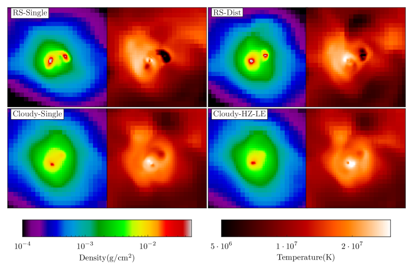
Figure 1.— Projections of gas column density (left panel in each pair) and gas density-weighted temperature (right panel) of the corresponding halo from the four simulations as labeled. The density and temperature color bars apply to all four pairs. “RS-Single” and “RS-Dist” employ metallicity-independent gas cooling, while “Cloudy-Single” and “Cloudy-HZ-LE” use metallicity-dependent cooling. Star particles in “RS-Single” and “Cloudy-Single” deposit all their feedback into the single cell that surrounds them, while stars in “RS-Dist” and “Cloudy-HZ-LE” use distributed feedback and deposit their feedback over the 27 cells that surround them. The projections are through a cube 2 Mpc on a side. The cluster has R${}_{200}\approx 1.9$ Mpc, M${}_{200}\approx 3.9\times 10^{14}$ M_⊙ and $T_{\rm vir}\approx 3.7\times 10^{7}$ K (using Eqn. 9).

Our first suite of simulations focus on the effects of Cloudy cooling (i.e., metal-dependent) and distributed feedback on simulations and observables. This is accomplished with four simulations beginning with an initial simulation similar to what was performed in B08. The only functional difference is a somewhat higher energy feedback parameter $\epsilon_{E}$: $4.11\times 10^{-6}$ in B08 versus $1.0\times 10^{-5}$ here. Our current value releases an amount of energy per unit stellar mass within a factor of two of several other similar studies of clusters (e.g. Kravtsov et al., 2005; Tornatore et al., 2007). A further difference is that in B08 each cluster is simulated in a separate zoom-in simulation, while in this work we simulate all of the clusters at once. This should not, however, lead to any meaningful differences because the mass and peak spatial resolutions, refinement criteria, and the physics modules are identical in the two cases.

We label the first simulation “RS-Single” (i.e. metal-independent cooling with feedback deposited in a single cell) to make clear which cooling and feedback modules are in use. The remaining three simulations (see Table 1) swap RS cooling in favor of Cloudy cooling (“Cloudy-Single”), swap single cell for distributed feedback (“RS-Dist”), or swap both (“Cloudy-HZ-LE”, which can be read as “Cloudy-High Metal Feedback-Low Energy Feedback”). We do not change anything else between simulations, and in particular, $\epsilon_{E}$ and $\epsilon_{Z}$ are kept constant between simulations. The figures in this section include all the gas in the central regions of the clusters, which may include cold gas invisible to X-ray observatories. We discuss the impact of the cold gas on our calculations in §4.5.

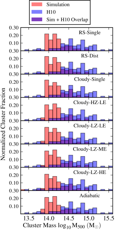
Figure 2.— Normalized distribution of M₅₀₀ for simulated and observed clusters. The colors are semi-transparent – dark blue indicates overlap between observation and simulation. The values of M₅₀₀ for H10 data are found using their Eqn. 4 and $kT_{\mathrm{vir}}$ from their Table 2. The simulations in the lower four panels are introduced and discussed in Sections 5 and 6.

Additionally, below we compare the observable quantities of our simulated clusters against the observations presented in H10. Figure 2 shows that our most massive clusters are less massive than the most massive observed clusters. Therefore, for purposes of comparing simulations to observations, a subset of the H10 sample has been selected to exclude clusters with M₅₀₀ values greater than the most massive simulated clusters. However, as we will discuss in §5.1, more massive simulated clusters do not exhibit substantially different behavior than the clusters discussed in this section. This selection eliminates 3 of 28 SCC clusters, 4 of 18 WCCs, and 5 of 18 NCCs from the observational sample, but does not greatly affect the overall ranges, nor distribution of observed central cooling time, entropy, or temperature ratio.

4.1. The Impact of Metallicity-Dependent Cooling

The left column of panels in Figure 1 visually compares RS-Single with Cloudy-Single using a representative cluster. This particular cluster is used because it is undergoing a single merger, which allows us to illustrate several important differences between simulations, but it is not overly complicated by multiple simultaneous mergers. It is clear that the choice of cooling method has a pronounced effect on the cluster. The Cloudy-Single cluster is less centrally dense than the same cluster in the other three models, and the infalling clump that is very cold in the RS-Single case is much warmer with smoother gradients in, e.g., Cloudy-Single. These differences are also evident in the temperature profiles shown in Fig. 3. At all radii, the mean Cloudy-Single cluster is warmer than the mean RS-Single cluster. Outside $0.1R_{500}$, the profiles are shifted by a nearly constant amount ($\sim 0.1$), which is a direct result of Cloudy cooling preventing unenriched gas at high redshift from becoming too cold. The large differences in temperatures inside $0.1R_{500}$ are also a result of the early overcooling of the RS method due to its assumption of relatively high metallicity at all times.

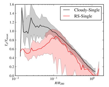
Figure 3.— The mean (solid lines) normalized temperature profiles for all Cloudy-Single (blue) and RS-Single (red) clusters and the $1\sigma$ scatter (semi-transparent filled regions).

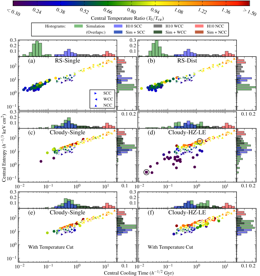
Figure 4.— Comparison of central cooling time, entropy, and temperature ratio for both simulated and observed clusters. Please see text for a detailed description of this figure. The circled points in panel (d) correspond to the two clusters in Fig. 9.

In Fig. 4 we compare simulations against observations, and by extension, to one other. Figure 4 contains a great deal of information and therefore warrants a detailed description. For a given simulation, there are three elements: the main panel and two histograms. The main panel (which has the largest area and contains the simulation label) shows the central cooling time versus entropy for both simulations and observations, with the simulated clusters represented by circles and the sub-selected H10 cluster sample represented by triangles. The H10 triangles are oriented according to the central cooling time subgroup cuts (SCC $\leq 1$ h^-1/2 Gyr, 1 $<$ WCC $\leq 7.7$, and 7.7 $<$ NCC). The colors of the glyphs in the main panel correspond to the central temperature ratio following the color scale along the top of the figure. Both above and to the right of each main panel are normalized histograms of central cooling time (above) and entropy (right) for simulations and H10 data. The colors of the histogram bars indicate the type of data plotted (simulated or H10 subgroups) following the histogram color key, which is above all the figure panels and below the color bar. The entropy histograms are cut according to SCC $\leq$ 22 $h^{-1/3}\ \mathrm{keV}\ \mathrm{cm}^{2}$, 22 $<$ WCC $\leq$ 150, and 150 $<$ NCC. Histogram bars are semi-transparent, and overlap between simulation and H10 data are indicated by the three darker colors in the histogram color key. Note that the entropy distributions for panels (a),(b), and (e) are highly peaked and one or more histogram bar extends beyond the displayed fractional range (0.25).

We can now remark on the profound effect Cloudy cooling has on the observables between panels (a) and (c) of Fig. 4. While central cooling times are much shorter than observed in the RS-Single case, Cloudy-Single clusters exhibit a much wider distribution of cooling times that are shifted to higher, more physically realistic values. A similar effect is seen in the central entropy values as well. However, despite the apparent visual improvement, non-parametric Kolmogorov-Smirnov (KS) (Kolmogorov, 1933; Smirnov, 1939) tests between data and simulation for these two observables gives $p$-values less than 0.01 (the typical lower cutoff for statistical similarity) for both RS-Single and Cloudy-Single, which indicates that none of the simulated distributions are statistically similar to observations. The short cooling times and low entropies with RS cooling are a direct result of early universal overcooling. The overall colder gas produces higher central cluster densities (Fig. 5), and lower central temperatures (e.g., Fig. 3) which, in the relevant temperature range ($\sim 10^{7}$ K), result in higher cooling rates (Eqn. 5). Note that Fig. 5 shows that outside the core, both methods of cooling produce cluster density profiles in rough agreement with observations, but that towards the core all simulations show central densities higher than observations, which is a typical problem with these kinds of simulations. The use of Cloudy cooling creates clusters with less unphysically high central densities than with RS cooling, but additional physical models (e.g. AGN feedback) may be required to address this discrepancy fully.

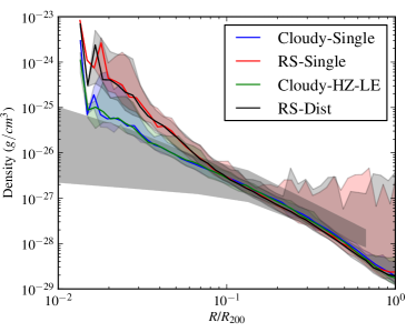
Figure 5.— Mean density profiles for each simulation (solid lines) with $1\sigma$ scatter (semi-transparent filled regions). The range of observed densities from Planck Collaboration et al. (2011) is over-plotted in grey.

In Figure 6 we compare the central temperature ratios of simulated and observed clusters. It’s clear that neither RS-Single (a) nor Cloudy-Single (c) are similar to observations. RS-Single is too cool and produces few NCC clusters, while Cloudy-Single is the opposite, with too many NCC clusters. Neither of the KS tests between these two simulations and the observed distribution of central temperature ratios give $p$-values greater than 0.01.

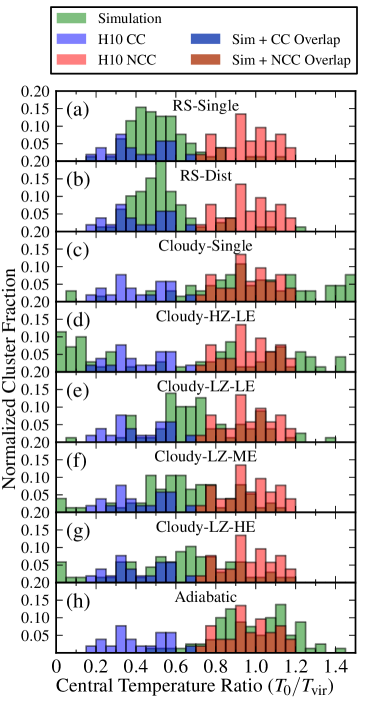
Figure 6.— Central temperature ratio histograms for simulated clusters (green) and observed clusters of comparable mass. The calculations for the simulated clusters do not include a temperature cut. The colors for observed data correspond to the bimodal groups NCC (red) and CC (blue) as defined by H10 (CC $\leq$ 0.7 = $T_{0}/T_{\mathrm{vir}}$). The simulations in the lower four panels are introduced and discussed in Sections 5 and 6.

4.2. The Impact of Distributed Supernova Feedback

Next, we study the effect of varying the spatial extent of thermal and metal feedback from supernovae (using RS cooling in both simulations). Figure 7 shows that the mean temperature profiles of RS-Single and RS-Dist are indistinguishable. This is a reasonable result because the addition of distributed feedback does not change the total amount of energy deposited into the gas by a given star particle. Interestingly, there are some differences that can be seen when the temperature projections are compared in Fig. 1. From RS-Single to RS-Dist, it appears that the amount of very cold gas in the infalling clump is somewhat diminished. This is consistent with the distributed energy feedback of merger-driven star formation more effectively heating the cold gas of the clump over a wider region. This same effect is seen in projections of other merging cold clumps in RS-Dist clusters. Note that although although the infalling clump has less cold gas with distributed feedback, the mass of the clump is low enough (and other merging clumps like it) that averaged over all the clusters, the warming effect is not enough to dramatically change the mean temperature profile between the two simulations.

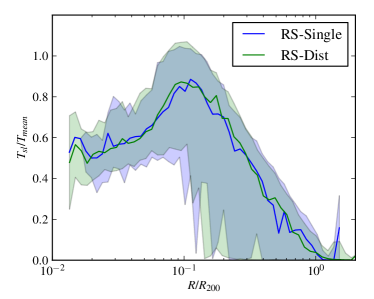
Figure 7.— Similar to Fig. 3, except the simulations used are RS-Single (blue line) and RS-Dist (green line).

The effect of distributed feedback on observables is smaller than the changes when Cloudy cooling is used, which is illustrated in Fig. 4. The distributions of central cooling times and entropies of the RS-Dist clusters are slightly widened, but do not resemble observations. Likewise, the spread of temperature ratios (Fig. 6) is slightly greater with distributed feedback, but again is not very similar to observations. Like RS-Single, none of the KS tests for RS-Dist indicate that the simulated distributions are statistically similar to observations. Considering all three observables together, it appears that distributed feedback has a slightly similar, but much less strong effect on the observables as does Cloudy. Namely, by distributing feedback over wider regions, including cold, tight clumps (like in Fig. 1) it acts to partially counter the RS overcooling and widen the distributions of the observables. The entropies for both RS simulations are low because nearly all the clusters have cool central temperatures and central densities higher than Cloudy simulations (Fig. 5). These two effects are both a consequence of early overcooling, and are complementary in Eqn. 8, resulting in low entropies.

4.3. The Impact of Combining Distributed Feedback + Metallicity-Dependent Cooling

Finally, we examine the result when both distributed feedback and Cloudy cooling are used simultaneously. Morphologically, the combination of Cloudy cooling and distributed feedback appears to only make small differences when compared to the substitution of only Cloudy. Indeed, the qualitative differences between rows of Fig. 1 are greater than the differences between columns. This highlights the importance of the addition of metallicity-dependent cooling due to its greater effect on the clusters when compared to the addition of distributed feedback. This is reasonable because distributed feedback is only operational when and where star particles are being formed, while Cloudy cooling makes substantial changes to cooling rates compared to RS cooling over the whole simulation at all times.

Figure 8 illustrates this point. Outside $0.1R_{500}$, which accounts for the bulk of the cluster, the temperature profiles are nearly identical. However, inside $0.1R_{500}$, where the star particles are applying feedback, the differences between Cloudy-Single and Cloudy-HZ-LE become much larger. In particular, the $1\sigma$ scatter of Cloudy-HZ-LE temperatures is much larger than it is for Cloudy-Single. Although Cloudy-Single produces approximately 25% more star particles by mass than Cloudy-HZ-LE (see Fig. 13 in §6.1), the ratio of total mass of metals (in star particles and in the gas) to the total mass of stars is the same within few percent in both simulations. The difference is that in Cloudy-HZ-LE, 19% of the metals by mass are stored in the gas, while this figure is only 10% for Cloudy-Single, which implies that the Cloudy-HZ-LE has $\sim 50$% more metals by mass in the gas than Cloudy-Single. The increased metals in the gas allows for much higher rates of cooling, giving rise to the scatter seen in Fig. 8.

The fact that more metals are stored in star particles in Cloudy-Single is very important. Although some of the metals given to star particles are recycled and enriched back into the gas after the particle is formed (see Eqn. 2), the metals that remain in star particles after the feedback is applied (e.g., after $12t_{\mathrm{dyn}}$) are locked in forever. Crucially, these metals are no longer available to contribute to cooling of the intracluster medium. The net effect is that, in comparison to the Cloudy-HZ-LE star particles, the Cloudy-Single star particles behave as a kind of “metal sink.”

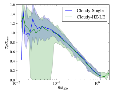
Figure 8.— Similar to Fig. 3, except the simulations used are Cloudy-Single (blue line) and Cloudy-HZ-LE (green line).

This result of enhanced metal feedback in the gas is a curious secondary effect of distributed feedback. It appears that without distributed feedback, the metals returned by star particles in each star-forming region stay contained within that region, and are re-captured by the next generation of star particles. Distributed feedback appears to disrupt this cycle because it deposits much of the metal-enriched gas outside star formation regions, preventing metals from being locked in star particles, and resulting in more metal mass in the intracluster medium. We compare the metallicities for these two simulations to observations in §4.4.

The impact of the higher metallicity and cooling in Cloudy-HZ-LE is starkly visible in Fig. 4(c,d). Instead of a tight linear grouping like the Cloudy-Single clusters, the Cloudy-HZ-LE clusters are scattered widely in central cooling time, entropy, and temperature ratio. Many clusters exhibit quite low cooling times, entropies, and extremely low central temperatures, and some of these “cold-core” clusters have $T_{0}/T_{\mathrm{vir}}$ much less than 0.01 and have central temperatures that drop below $10^{6}$ K. The cold-cores are tightly bunched at the low end of the distribution in Fig. 6(d). It is these cold-cores that give rise to the scatter in Cloudy-HZ-LE cluster temperature profiles inside 0.1 $R_{200}$ (Fig. 8). As with the earlier simulations, none of the Cloudy-HZ-LE distributions are statistically similar to observations according to the KS test. We note that in reality, X-ray observations cannot detect the cold gas present in the cold-cores, which we discuss in more detail in §4.5.

Using a halo merger tree we examine the evolution of the clusters, and, in particular, focus on the central temperature histories of the cold-core clusters. As we found in B08, after formation all of the clusters in our calculations eventually become CC clusters with low central temperatures. Later on, some of the clusters experience major mergers, which may disrupt the embryonic cool core, and raises the central temperatures permanently. However, some clusters grow by only minor mergers and smooth accretion early on, and the low central temperatures can be preserved to z=0, although they may encounter large impact parameters and/or minor mergers at late times. These later mergers are insufficient to destroy the large and tightly-bound cool core, and only act to add more cool gas to the core.’ With the addition of Cloudy cooling, and the enhanced distribution of metals from distributed feedback algorithm, the Cloudy-HZ-LE clusters that might have stayed simply cool are in fact able to become cold. This is illustrated for two Cloudy-HZ-LE clusters in Fig. 9, where the central temperature ratio is shown along with major merger events over time. Note that the mass-scaling relation used to calculate T_vir elsewhere in this paper is not used in this figure because at early times the mass and redshift of the clusters falls outside the applicable range of the scaling relation. Instead, T_vir is calculated by finding the spectroscopic-like temperature inside $R_{200}$, but with the core removed. At z=0 this T_vir is roughly similar to the mass-scaled T_vir. In Fig. 9 the cluster that ends up warm at z=0 is cool from z$\approx$3 to z$\approx$1.3, but then undergoes two mergers in quick succession around z$\approx$1.3. After a period of mixing, over which the core temporarily drops in temperature, the central temperature rises and never re-cools. In contrast, the cold cluster experiences no major mergers early in its formation, which allows the cold core to be established. It does experience several mergers later in its evolution, but they happen after the cold core has become established and too gravitationally bound to be destroyed by the energy of the various mergers. We stress that while this scenario of the simulated cool/cold-core clusters surviving late major mergers may be inconsistent with observations that show clusters with recent major mergers lack cool cores (e.g., Rossetti et al., 2011), late mergers impacting CCs is not a requirement of our model.

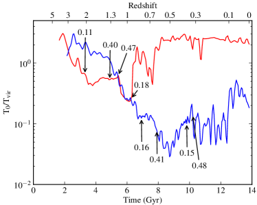
Figure 9.— T₀/T_vir as a function of time for the two Cloudy-HZ-LE clusters indicated by circles in Fig. 4(d). The red line corresponds to the warm cluster in the upper right, and the blue to the cold cluster in the lower left. The downward-pointing arrows show major (M_subhalo/M_cluster $\geq$ 0.1) merger events for the warm cluster. Likewise, the upward arrows are for the cold cluster. The number with each arrow is the M_subhalo/M_cluster ratio for that merger. At z=0 the warm cluster has M${}_{200}\approx 6.0\times 10^{14}$ M_⊙, and the cold cluster has M${}_{200}\approx 1.5\times 10^{14}$ M_⊙.

4.4. Metallicity

We have just shown that simulations using RS (metallicity-independent) cooling fail to reproduce the observed central quantities due to unphysically high levels of cooling early in the cluster evolution. Unfortunately, using a metal-dependent cooling algorithm does not result in realistic clusters either. It is known that a bimodality exists between CC and NCC clusters in which NCC clusters exhibit a flat metallicity profile towards the center while CC clusters show an enhancement in the core (De Grandi & Molendi, 2001; Böhringer et al., 2004; Baldi et al., 2007; Johnson et al., 2011). Clearly, gas metallicity is a very important quantity to examine when attempting to understand CC/NCC clusters, and in Fig. 10 we compare the metal profiles of both Cloudy simulations to observations (Matsushita, 2011). These observations, done with the using XMM-Newton satellite, estimate metallicity by measuring the strength of iron lines as function of radius in 28 clusters, 20 of which are also in H10 sample. Fig. 10 mirrors the earlier finding that the Cloudy-HZ-LE simulation has higher mean metallicity than Cloudy-Single, but it also shows two important differences between simulations and observations. First, the central ($\lesssim 0.07R_{200}$) metallicities of both Cloudy simulations are far too high, and second, the slopes of the profiles are far too steep with too little metallicity outside $\gtrsim 0.07R_{200}$. Both effects have been noted before in simulations with star formation + cooling and without AGN feedback (e.g., Sijacki & Springel, 2006).

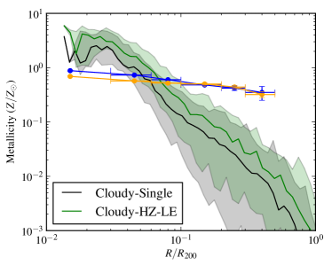
Figure 10.— Mean Cloudy-Single and Cloudy-HZ-LE metallicity profiles (solid lines) and $1\sigma$ scatter (semi-transparent shaded regions). Observed data from Matsushita (2011) is shown with error bars; blue for clusters with a cD galaxy, and orange for those without.

Both effects are caused by star formation that is too centrally concentrated. Nearly all of the star formation occurs inside $0.1R_{200}$ in the region of the cluster with the highest gas density, which implies that essentially all of the thermal feedback is contained within this region. This effect is still present when distributed feedback is used, since the region over which feedback takes place for each star particle is a cube $\approx 47h^{-1}$ kpc on a side – significantly smaller than the volume contained within $0.1R_{200}$. Given the high density of the gas, cooling takes place rapidly, lowering the entropy of metal-enriched gas and keeping it contained within the center of the cluster. In principle, star formation in galaxies near the outskirts of clusters could result in substantial additional enrichment of the gas. In practice, however, the relatively low resolution of these calculations prohibits star formation in all but the largest galaxies in a cluster, resulting in highly centralized star formation. As a result of these two factors, the metallicity profile in all of our simulated galaxy clusters is heavily tilted, with the inner regions of the clusters having far too much metal, and the outer regions having too little.

4.5. The Effect of Cold Gas on Observables

The orbiting X-ray observatories Chandra and XMM-Newton have little to no sensitivity below $\approx 0.5$ keV, which means that they are unable to accurately detect gas colder than a few million K (Garmire et al., 2003; Jansen et al., 2001). The simulated cold-core clusters discussed earlier in this section contain gas at their center well below this temperature threshold, which means that the cold gas would be invisible to the observatories. Therefore, to more accurately model observables as they might be measured by the aforementioned observatories, it is appropriate for the calculations of the observables to remove the cold central gas from consideration (Nagai & Lau, 2011). As described in Section 3.2.1, mock X-ray measurements like $T_{spec}$ are unphysical at these low temperatures. Calculations of the metallicity and other X-ray derived quantities from simulations are likewise skewed if this non-X-ray emitting gas is included.

The removal of cold gas from the calculation is accomplished for each cluster by first finding the total central X-ray emissivity in the 0.5-7.0 keV bandpass. Next, we find the temperature for which gas below that temperature accounts for only 5% of the total emissivity. We then eliminate the gas below this threshold from our calculations of all three main observables. The mean temperature cut across all clusters is roughly $1-2\times 10^{7}$ K, which is very similar to the lower temperature limit of the observatories quoted earlier. We show the result of these temperature cuts for two simulations, Cloudy-Single and Cloudy-HZ-LE, in Fig. 4(e, f). We note that when we perform this same temperature cut procedure on the other simulations (not plotted), the differences in the observables are negligible because those simulations contain very little or no gas below $1-2\times 10^{7}$ K in the centers of the clusters.

With the temperature cuts, the cold-core clusters disappear, and the simulations appear more similar to observations (see panels (e, f) of Fig. 4). In fact, Cloudy-HZ-LE without cold gas produces a distribution of central cooling times just on the cusp of being likely to be consistent with observations ($p$=0.01). However, we argue that this improvement is of mixed value for analyzing these simulations. While the cold-core clusters do appear more realistic using the temperature cuts, it hides the true nature of the cold gas which is unlikely to be physical. For example, Hicks et al. (2010) find using UV GALEX observations of CC clusters (some of which are in the H10 sample) that star formation rates in the inner 50-100 kpc are generally well under 1 M_⊙/yr. The low rate of star formation in observed CC clusters indicates that there is not a large amount of very cold gas present in the centers of CC clusters. Because the cold gas is therefore unlikely to be physical, and clusters without the unphysical cold gas are unaffected by the temperature cuts, the inclusion of the cold gas in our calculations is actually more informative for purposes of understanding the simulations and identifying problematic clusters. Therefore, we will include the cold gas in our calculations for the remainder of our analyses.

5. The Effect of Varied Feedback and Cluster Mass on Observables

The results presented in the previous demonstrate that simply changing radiative cooling methods and the way that stellar feedback is deposited into the intracluster medium cannot produce physically-reasonable simulated clusters that agree with observations. Therefore, we move on to varying the quantities of feedback into the ICM from supernovae, which are remaining free parameters in our model. The results from Section 4 indicate that the RS cooling results (using a metallicity-independent cooling table) fail to produce realistic clusters, which leaves the Cloudy (e.g., metallicity-dependent cooling) simulations as options for a platform for further exploration. It is arguable which of the two Cloudy cooling simulations better reproduce observations, but we choose to use Cloudy-HZ-LE as the basis for further testing because it employs both metallicity-dependent cooling and the distributed stellar feedback algorithm. The Cloudy cooling has no adjustable parameters, leaving only the feedback parameters $\epsilon_{E}$ and $\epsilon_{Z}$.

Because the central metallicity of Cloudy-HZ-LE is so much higher than observations, and it is clear that the high metallicity has a large effect on the observable properties of the simulated cluster cores, we run three simulations in which we lower the metal feedback parameter ($\epsilon_{Z}$) by a factor of five, and we vary the value of the energy feedback parameter ($\epsilon_{E}$) (see Table 1). These three simulations are labeled “Cloudy-LZ-LE” (“Cloudy-Low Metal Feedback-Low Energy Feedback”), “Cloudy-LZ-ME” (Medium Energy Feedback), and “Cloudy-LZ-HE” (High Energy Feedback). The first of the three has the same value of $\epsilon_{E}$ as Cloudy-HZ-LE, while the next two increase $\epsilon_{E}$ by a factor of 8 and 20, respectively.

Figure 11 shows that the lower $\epsilon_{Z}$ has dramatically reduced the central metallicities in all three simulations. Indeed, inside roughly $0.05R_{200}$ (which includes our defined central region), the Cloudy-LZ-LE metallicities agree fairly well with observations. However, outside that region the metallicity still declines far too rapidly for all three simulations. This is not surprising since, to first order, we have simply reduced the amount of metal that is produced overall in the simulation, but not the locations or timing of star formation.

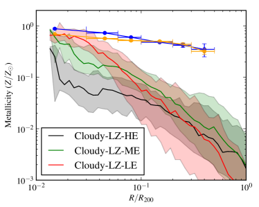
Figure 11.— Mean metallicity profiles for all three low metal Cloudy runs (solid lines) and $1\sigma$ scatter (semi-transparent filled regions). Observed data from Matsushita (2011) is shown with error bars; blue for clusters with a cD galaxy, and orange for those without.

In Figure 12 we show the results of varying the feedback energy on our observables. The figure shows that the lower and more realistic central metallicities have a profound effect on the observables. From Cloudy-HZ-LE (Fig. 4(d)) to Cloudy-LZ-LE, the very low entropy tail of Cloudy-HZ-LE has vanished, and in its place the central entropy distribution is now peaked solidly, but too strongly, in the observed SCC range. Additionally, lowering the metal feedback has significantly altered the distribution of central temperature ratios (Fig. 6(e–g)), and brought them closer to agreement with observations. In particular, the KS test between observations and the Cloudy-LZ-LE central temperature ratio distribution gives $p=0.03$, which is the best match out of all the distributions presented in this paper.

The other two low-metallicity runs show that by adjusting the feedback parameters, we are able to produce more realistic clusters, at least as measured by these three observables. In particular, except for a few simulated cold-core clusters (which we discuss below), the agreement between the observed SCC+WCC distributions of central cooling time and of entropy and the Cloudy-LZ-HE clusters is visually better than any of the other simulations. As in all other simulations, KS tests produce $p$-values less than 0.01, but this is largely due to our inability to produce clusters with NCC-like cooling times and entropies.

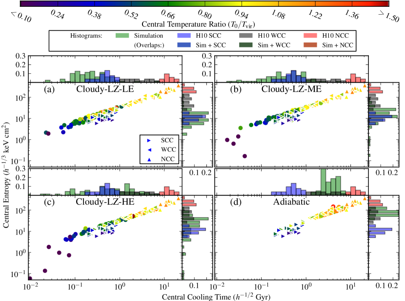
Figure 12.— Plots and histograms of central cooling time and entropy for simulated and observed clusters; similar to Fig. 4. See §4 for a detailed description of the aspects of this figure. Gas temperature cuts have not been applied to the calculations in this figure. The “Adiabatic” simulation is discussed in Section 6.3.

These three low metallicity simulations produce a few interesting trends that allow us to highlight the interconnectedness of star formation, gas enrichment, and gas cooling that is at the core of our inability to produce a realistic distribution of clusters. First, the simple act of reducing the metal feedback from Cloudy-HZ-LE to Cloudy-LZ-LE noticeably shifts the distributions of cooling times and entropies to lower values. This is a direct result of the fact that lowering the amount of metals in the gas reduces gas cooling, and this in turn reduces the star formation rate (see Fig. 13). Lower rates of star formation reduces the amount of energy feedback available for raising the central cooling times and entropies. We discuss Figure 13 in more detail in Sections 6.1 and 6.2.

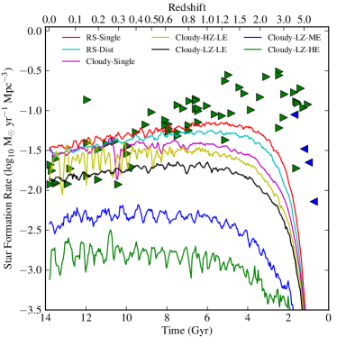
Figure 13.— Star formation rates over time for each simulation. We plot observed rates as a visual guide, but we do not expect concordance. The simulated rates have been smoothed by averaging over a moving window $\sim 200$ Myr wide. The blue left-pointing triangles are observed rates from Bouwens et al. (2007), and the green right-pointing are from Hopkins (2004, 2007). Error bars have been omitted from the observations for clarity.

Second, as $\epsilon_{E}$ is increased, the bulk of the central cooling times and entropies moves to greater values, and becomes more in line with the SCC+WCC portion of the observed distributions. This is not a surprising effect. Raising the energy feedback of star formation acts to heat up the gas, which raises cooling time, and also increases the entropy. Note that despite increasing $\epsilon_{E}$ by a factor of 20, we still fail to produce fully-NCC (i.e. in the NCC range of all three central quantities) clusters.

Curiously, increasing the energy feedback also increases the number of very low entropy, cold-core clusters from Cloudy-LZ-LE to Cloudy-LZ-HE. In contrast to the Cloudy-HZ-LE cold cores, which are primarily due to the high metallicity of the ICM in the center of the cluster, the increase in the number of cold cores seen in the Cloudy-LZ-HE simulation are due to a combination of low metallicities and low amounts of formation of stars and their associated feedback energy. Figure 14 shows that the coldest Cloudy-LZ-HE clusters also have relatively low total stellar masses. In the higher energy feedback run, it appears that the high thermal feedback of a given generation of stars inhibits the formation of the next generation of stars, forming a feedback loop. In some clusters this feedback loop is very strong, and despite (and due to) the high value of $\epsilon_{E}$, the star formation is not enough to warm up the core. This suppression of star formation as feedback energy is increased is also illustrated in Fig. 13.

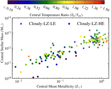
Figure 14.— The central mean metallicity versus total central stellar mass for Cloudy-LZ-LE and Cloudy-LZ-HE.

Third, while the central cooling times and entropies shift as the thermal feedback is modified, the central temperature ratios (Fig. 6(e–g)) do not change nearly as much (except for the addition of the few cold-core clusters at the cold end of the distributions). The reasons why the central temperatures do not change very much with $\epsilon_{E}$, while the cooling times and entropies do, are complex. Figures 11 and 13 show that the increase in $\epsilon_{E}$ lowers both the central metallicities and star formation rates. This results in lower cooling rates which prevents central densities from becoming quite as high (see 15). Keeping roughly equal temperatures, but having lower densities, results in longer cooling times and higher entropies. Across the three simulations the temperatures stay roughly equal because, despite the factor of 20 increase in the amount of thermal energy returned to the intracluster medium per solar mass of star formed, the amount of feedback energy returned to the gas stays strikingly constant (Fig 16). From Cloudy-LZ-LE to Cloudy-LZ-HE, there is less than a factor of two increase in total energy deposited in the gas. Figure 16 is discussed in more detail in §6.3.

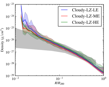
Figure 15.— Mean density profiles for each simulation as labeled (solid lines) with $1\sigma$ scatter (semi-transparent filled regions). The range of observed densities from Planck Collaboration et al. (2011) is over-plotted in grey. These density profiles are essentially unchanged from the earlier simulations using Cloudy cooling (Fig. 5).

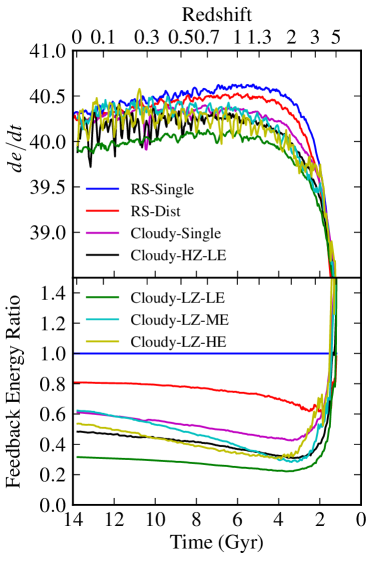
Figure 16.— Top panel: Instantaneous feedback energy over time averaged over a moving window $\sim 200$ Myr wide. The units are in $\log_{10}($ergs s^-1 Mpc${}^{-3})$. Bottom panel: Full-box total energy feedback integrated over time, as a function of time, for each simulation divided by the same for RS-Single (hence RS-Single in blue is a flat line).

5.1. Higher Mass Clusters

Above and in §4 we removed 12 clusters from the H10 sample because their masses are higher than the most massive ones in our simulations. Due to their deeper potential wells and likely richer history of mergers, it is reasonable to expect that higher-mass clusters would tend toward having NCCs when compared to less massive clusters. In order to test if higher-mass clusters behave differently than the ones already discussed, we ran a suite of follow-up simulations of higher-mass clusters. The higher mass clusters do not show any meaningful changes in their physical observables when compared to their lower mass analogues, indicating that simply producing higher mass clusters does not produce more realistic clusters.

6. Discussion

In this paper, we have shown that Cloudy (metallicity-dependent) cooling and distributed thermal feedback can be used to create simulated galaxy clusters with somewhat more realistic ICM properties than in previous generations of simulations. Even our best models, however, fail to accurately reproduce the observed cluster properties – in particular, the distribution of clusters into cool core and non-cool core clusters and related properties: the central entropy and cooling time of the intracluster gas, the ratio in temperature of this central gas from the cluster’s virial temperature, and the distribution of metals within the cluster itself. In particular, virtually none of our simulated clusters fall into the non-cool core ranges of central cooling time and entropy. In this section, we discuss possible reasons for the continued difference between our simulation clusters and real galaxy clusters.

As discussed in the introduction to this paper, there is a large body of numerical work that shows that AGN can help to alleviate some of the problems exhibited by our simulations, including regulating star formation and promoting the distribution of metals. In Section 7 we discuss a sub-grid feedback method that we believe will allow us to address the some of problems discussed in this section and should allow us to include AGN feedback to our clusters as well.

6.1. Lack of Resolution

Due to finite computational resources and the need to simulate a large volume of the Universe, our galaxy cluster simulations have relatively poor mass and spatial resolution compared to the current cutting-edge in galaxy or single-cluster (e.g., Li & Bryan 2012) formation simulations. This has a negative effect on the accuracy of our model, and is especially true at early times, when cooling and star formation is taking place in real galaxies with masses below the resolution of these simulations. For example, at z$\approx 6$ the dominant galaxy population in terms of feedback is $\approx 10^{10}-10^{11}$ M_⊙ (Bouwens et al., 2007; González et al., 2011), and at z=2 it is $\approx 10^{12}$ M_⊙ (Conroy & Wechsler, 2009). Given that the dark matter particle mass in our simulations is $7.8\times 10^{9}$ M_⊙, we simply cannot resolve galaxies at high z, and therefore we do not make stars at that epoch. This is clearly illustrated in Fig. 13. Furthermore, in Enzo, as in hydrodynamical simulations in general, gas cooling within halos only becomes significant once once the gravitational potential is well-resolved, and thus can compress gas to high densities and form stars. From a practical standpoint, this means that a halo must contain a relatively large number of dark matter particles before star formation can occur – substantially more than is required to simply register the existence of a halo. This is illustrated by the fact that in these simulations the average halo has a mass of $7.3\times 10^{12}$ M_⊙ when a star is first formed inside it, which corresponds to $\approx 1,000$ dark matter particles. Because the halos that form stars for the first time are so massive, star formation occurs later in time and in objects with deeper potential wells (and thus denser gas) than is typical in the real Universe. The denser gas is able to cool more readily, which means that the thermal feedback from star formation does not warm up gas as effectively, and the overall result is an excess of cooling and a deficit of entropy at low redshifts. The injection of metals into the intergalactic medium is similarly affected by our lack of resolution, with metal-enriched gas being more strongly concentrated than is observed. This leads to an unfortunate feedback loop – stars form too late and in over-dense regions, which are then over-polluted with metals. This excess of metal in the gas causes cooling to occur too rapidly, reducing or eliminating the pressure gradients that would drive metal-enriched gas to large cluster radii.

The star formation rate in our simulations is illustrated in Figure 13. Observed data from Bouwens et al. (2007) (from the HST HUDF and GOODS fields) and Hopkins (2004, 2007) (combined from the literature) are included in the figure for comparison. This illustrates that all of the calculations discussed in this paper differ substantially from observed rates at z$>$0.3, and in some cases do so quite dramatically. Of course, as mentioned above, the simulations do not resolve the galaxies that are responsible for a large fraction of star formation, and therefore it is unreasonable to expect precisely matching rates. Rather, the figure confirms that star formation begins later than the cosmic mean, which is exactly the opposite of what one would expect from observations of galaxy clusters, where the bulk of stars form earlier than the cosmic average due to clusters being substantially over-dense regions at high redshift.

6.2. Interconnectedness of Star Formation and Feedback

A striking feature of the different stellar histories in Fig. 13 is how much they change as the models for radiative cooling and subgrid star formation are adjusted. Every deliberate choice we made to improve the distributions of our three core observables has, in fact, caused the timing of the peak rate of star formation to occur later and later. Recall that this is contrary to what is desired, which is a cluster star formation rate peak that occurs earlier than the overall universal peak. This effect, and the effects noted earlier of adjusting $\epsilon_{E}$ and $\epsilon_{Z}$, illustrate the interconnectedness of star formation and feedback in our simulations.

An example of this effect are the low-metallicity runs discussed in §5. The first run, Cloudy-LZ-LE, that only reduces the metal feedback, results in clusters that have systematically low central entropies and cooling times. Increasing the energy feedback does somewhat ameliorate those particular discrepancies, but the result is an even less realistic history of star formation. It is clear that the star formation $\rightarrow$ metal feedback $\rightarrow$ gas cooling cycle is a self-reinforcing cycle. A logical change to one aspect of our subgrid stellar model results in other aspects drifting further from the observational results we are attempting to match. As mentioned previously, the cold-core clusters seen in Cloudy-LZ-HE are evidence of an incorrectly modeled cycle of star formation and metal enrichment. This same behavior exists in all the other simulations discussed in this work, and it is impossible to disentangle a change in one part of that cycle without affecting all the others, often negatively.

More broadly, the fundamental challenge with our subgrid models for star formation and feedback is their strong dependence on the mass and spatial resolution of the simulation, as was discussed in Section 6.1. Using our current technique, we will not be able to correctly resolve the early evolution of the galaxy populations in proto-cluster regions, which limits our ability to bring the observable properties of our simulated clusters in line with real galaxy clusters. Given this unresolvable issue, it is clear that a fundamentally different approach needs to be taken, which we will elaborate upon below.

6.3. Energetics

Our lack of fully-NCC clusters indicate that we are not correctly applying thermal feedback to these simulations. As an experiment, we run a simulation that has identical initial conditions and simulation parameters to the other calculations described in this paper, except that radiative cooling, star formation, and stellar feedback are all disabled. We label this calculation “Adiabatic,” and the results are shown in Figures 6(h) and 12(d). The only source of cooling in this calculation is from adiabatic expansion of the plasma, and the only sources of heating comes from adiabatic compression and from shock heating, powered by gravitational potential energy. As can be seen in Figures 6(h) and 12(d), the Adiabatic simulation results in warm galaxy cluster cores, with the majority of simulated clusters solidly in the NCC range of the central temperature ratio distribution (Fig. 6(h)). However, the central cooling times (as before, calculated using a cooling curve based on an optically thin plasma with a metallicity of 0.5) and entropies are only in the WCC ranges (Fig. 12(d)), which shows that simply heating the core to NCC-like temperatures is not enough to produce fully-NCC clusters. The Adiabatic results also highlight the requirement that clusters include both heating and cooling because without the early cool phase of clusters, some of which become may NCC clusters following mergers, it is impossible to create the full spectrum of cluster types.

We now turn to Figure 16, which demonstrates the insensitivity of the observables in our simulations to our choice of cooling algorithm and magnitude of both metal and thermal feedback. The instantaneous energies are calculated for each simulation by convolving the star formation rate (Fig. 13) with Eqn. 1 and the value of $\epsilon_{E}$ (Table 1). Following the rates in the top panel, the maximum instantaneous ratio between any two simulations is under an order of magnitude. The bottom panel is perhaps even more interesting. This shows that across all seven simulations the total feedback energies deposited in the gas are remarkably similar. From the highest total in RS-Single, to the lowest in Cloudy-LZ-LE, there is only about a factor of three change in the amount of energy deposited, which stands in stark contrast to the large changes in physics modules and feedback parameters. This shows that using our current tools it is very difficult to change the energy feedback history, and that it is likely very challenging to simulate the required energy feedback history to produce realistic clusters with the parameters we are able to adjust.

Despite the assertions above about little energetic differences between simulations, there are significant differences in the observables across the simulations. The fact that even small changes in energetics lead to major shifts in (especially) entropy and cooling time highlights the importance of accurately modeling energy physics in cluster simulations. As mentioned before, we discuss in §7 a method that should allow us to more accurately model the energetics in clusters and reproduce more realistic results.

7. Conclusions and Future Work

Where are we along the road to making realistic galaxy clusters? In Table 2 we summarize qualitatively the successes and failures of our seven main simulations, basing our statements on the data contained in Figures 4, 6, and 12. Since no simulations produced fully-non-cool clusters (as defined by the measured cooling times and entropies), we omit that as a comparison from the table, and note that it is a failure of all the simulations. However, we also note that all simulations, except those using metal-independent RS cooling, did produce a substantial fraction of NCC clusters as measured by central temperature ratio. Where we feel the judgment is warranted, we have labelled assessments with either a “best” or a “worst.” Our assessments of the three main observables illustrate that overall none of the simulations did particularly well at reproducing the observed distributions. The simulations using cooling tables that assume a constant, high metallicity (the RS series of runs) are the furthest from matching observations, primarily due to over-cooling of gas. Among runs using metal-dependent cooling (the Cloudy series of runs), the simulation with the low metal feedback and high thermal energy feedback (Cloudy-LZ-HE) overall produces the best match to observations, with reasonable agreement for both cooling time and decent agreement for both cooling times and entropies, and central temperatures almost entirely within the observed range, although the full spectrum of cool-core and non-cool core cluster is not reproduced.

Table 2Simulation Successes and Failures

Simulation Label	Cooling Time	Entropy	Temperature Ratio	Metallicity Profile	Star Formation
RS-Single	Worst, Entirely	Mainly Too Low	Mostly CCs,	N/A	Best Overall, Too Low
	Too Short		Too Few NCCs		Early, Too Slow Rolloff
RS-Dist	Mainly Too Short	Mainly Too Low	Mostly CCs,	N/A	Too Low Early,
			Too Few NCCs		Too Slow Rolloff
Cloudy-Single	Best SCC+WCC	Too Peaked Between	Too Many NCCs,	High in Center,	Too Low Early,
	agreement	SCCs and WCCs	Too Few CCs	Profile Too Steep	Too Slow Rolloff
Cloudy-HZ-LE	Decent SCC+WCC,	Many Cold-Cores With	Too Bimodal	Worst, Far Too High in	Far Too Low Early,
	But A Few Too Low	Too Low Values		Center, Profile Too Steep	Too Slow Rolloff
Cloudy-LZ-LE	Generally Too Short	Mainly SCCs,	Peaked Between the	Best in Center, Low in	Far Too Low Early,
		A Few WCCs	CC & NCC Groups	Periphery, Profile Too Steep	Too Slow Rolloff
Cloudy-LZ-ME	Mainly SCC,	Almost Entirely	Peaked Between the	Low in Periphery,	Far Too Low Early,
	A Few WCCs	WCCs	CC & NCC Groups	Profile Too Steep	No Rolloff
Cloudy-LZ-HE	Decent SCC+WCC,	Decent SCC+WCC,	Peaked Between the	Low Overall,	Worst, Abysmal Always,
	A Few Too Short	A Few Too Low	CC and NCC Groups	Profile Too Steep	No Rolloff

Note. — The entries are qualitative assessments of how well the simulations agree with observations.

We have also included assessments of the metallicities and star formation histories of the simulations in Table 2. In short, they generally fail to agree with observations. In terms of metallicity, Cloudy-LZ-LE is the best because it has central metallicities that are in relatively good agreement with observations. That said, this calculation, like all the other simulations, shows too steep a gradient in the metal profile at larger radii. With regards to star formation rate, none of our simulations accurately capture the star formation history one expects from galaxy clusters: the overall rate of star formation is too low, and peaks at too late of a time, compared to the rates inferred from observations of cluster galaxies.

Notwithstanding the qualitative assessments above and in the table, some of our results are encouraging. The inclusion of metallicity-dependent cooling rates significantly improves upon previous work that uses a cooling table that assumes a fixed, relatively high metallicity, and we show that it is possible to adjust simulations to achieve better specific agreement with observations. Clearly, a metal-dependent cooling method, like the method of Smith et al. (2008, 2011), is essential to prevent early overcooling of unenriched gas. Using a distributed feedback model, rather than depositing all of the thermal energy from supernovae into a single cell, does not have as large of an effect on cluster properties as cooling. In addition, we find that while metallicity profiles as a function of radius can be altered somewhat based on choices of feedback parameters, the metallicity profiles never resemble cluster observations. This points to the need for a more sophisticated feedback model that may include AGN feedback. Taken as a whole, these results begin to indicate a way forward that uses metallicity-dependent cooling, and which also addresses the shortcomings of the star formation and feedback model employed in this paper.

We conclude that our current methodologies are not capable of reproducing all observed properties of real clusters. Therefore, the next step on the road to more realistic clusters is to employ new physical models that address the shortcomings discussed in this paper. In particular, it is clear that we must address the unrealistic star formation histories and metallicity profiles of the clusters. Without improvements to both, it will be impossible to simulate the energetics of heating and cooling of observed clusters.

The method we believe will provide substantial improvements to our current methods are “galaxy particles” (also called “galaxy constructs”, or “galcons,” Arieli et al., 2008, 2010). Galaxy particles employ a model where the the time evolution of mass, metal, and energy feedback of galaxies are derived from the observed globally-averaged star formation rate, and the feedback quantities are deposited into the intergalactic medium isotropically and over a sphere whose radius is substantially larger than the cell size of the simulation, thus potentially avoiding the over-cooling. Arieli et al. (2010) compares a cluster simulation employing galaxy particles to one similar to RS-Single (in particular, in terms of cooling and feedback models). They find that galaxy particles are more effective at depositing mass, energy, and metals into the intracluster medium which results in more realistic temperature, density, metallicity, and entropy profiles. They find that galaxy particles help reduce the amount of subhalo “over-merging” in clusters, which reduces the central dominance of the simulated cluster. An additional advantage of such a technique is that it will allow us to include, in a parametric way, more complex physics such as AGN feedback and merger-driven starburst events. If successful, one could then use a wider range of cluster observables (e.g., the Sunyaev-Zel’dovich effect or L_X-T relationship) to further constrain calculations. Galaxy particles are presently being worked on by the Enzo development community, and we will present the results of cluster simulations using galaxy particles in a future paper.

References

- Abel et al. (1997) Abel, T., Anninos, P., Zhang, Y., & Norman, M. L. 1997, New A, 2, 181
- Agertz et al. (2007) Agertz, O., Moore, B., Stadel, J., et al. 2007, MNRAS, 380, 963
- Anninos et al. (1997) Anninos, P., Zhang, Y., Abel, T., & Norman, M. L. 1997, New A, 2, 209
- Arieli et al. (2008) Arieli, Y., Rephaeli, Y., & Norman, M. L. 2008, ApJ, 683, L111
- Arieli et al. (2010) —. 2010, ApJ, 716, 918
- Ashman et al. (1994) Ashman, K. M., Bird, C. M., & Zepf, S. E. 1994, AJ, 108, 2348
- Baldi et al. (2007) Baldi, A., Ettori, S., Mazzotta, P., Tozzi, P., & Borgani, S. 2007, ApJ, 666, 835
- Binney & Tabor (1995) Binney, J., & Tabor, G. 1995, MNRAS, 276, 663
- Böhringer et al. (2004) Böhringer, H., Matsushita, K., Churazov, E., Finoguenov, A., & Ikebe, Y. 2004, A&A, 416, L21
- Borgani (2004) Borgani, S. 2004, Ap&SS, 294, 51
- Bouwens et al. (2007) Bouwens, R. J., Illingworth, G. D., Franx, M., & Ford, H. 2007, ApJ, 670, 928
- Brickhouse et al. (1995) Brickhouse, N. S., Raymond, J. C., & Smith, B. W. 1995, ApJS, 97, 551
- Burns et al. (2008) Burns, J. O., Hallman, E. J., Gantner, B., Motl, P. M., & Norman, M. L. 2008, ApJ, 675, 1125
- Cardiel et al. (1998) Cardiel, N., Gorgas, J., & Aragon-Salamanca, A. 1998, MNRAS, 298, 977
- Cen & Ostriker (1992) Cen, R., & Ostriker, J. P. 1992, ApJ, 399, L113
- Chen et al. (2007) Chen, Y., Reiprich, T. H., Böhringer, H., Ikebe, Y., & Zhang, Y.-Y. 2007, A&A, 466, 805
- Conroy & Wechsler (2009) Conroy, C., & Wechsler, R. H. 2009, ApJ, 696, 620
- Cowie & Binney (1977) Cowie, L. L., & Binney, J. 1977, ApJ, 215, 723
- De Grandi & Molendi (2001) De Grandi, S., & Molendi, S. 2001, ApJ, 551, 153
- Dennis & Chandran (2005) Dennis, T. J., & Chandran, B. D. G. 2005, ApJ, 622, 205
- Di Matteo et al. (2005) Di Matteo, T., Springel, V., & Hernquist, L. 2005, Nature, 433, 604
- Eckert et al. (2011) Eckert, D., Molendi, S., & Paltani, S. 2011, A&A, 526, A79
- Eckert et al. (2012) Eckert, D., Vazza, F., Ettori, S., et al. 2012, A&A, 541, A57
- Edge (2001) Edge, A. C. 2001, MNRAS, 328, 762
- Eisenstein & Hu (1999) Eisenstein, D. J., & Hu, W. 1999, ApJ, 511, 5
- Fabian (1994) Fabian, A. C. 1994, ARA&A, 32, 277
- Fabian & Nulsen (1977) Fabian, A. C., & Nulsen, P. E. J. 1977, MNRAS, 180, 479
- Fabjan et al. (2011) Fabjan, D., Borgani, S., Rasia, E., et al. 2011, MNRAS, 416, 801
- Fabjan et al. (2010) Fabjan, D., Borgani, S., Tornatore, L., et al. 2010, MNRAS, 401, 1670
- Ferland et al. (1998) Ferland, G. J., Korista, K. T., Verner, D. A., et al. 1998, PASP, 110, 761
- Frenk et al. (1999) Frenk, C. S., White, S. D. M., Bode, P., et al. 1999, ApJ, 525, 554
- Garmire et al. (2003) Garmire, G. P., Bautz, M. W., Ford, P. G., Nousek, J. A., & Ricker, Jr., G. R. 2003, in Society of Photo-Optical Instrumentation Engineers (SPIE) Conference Series, Vol. 4851, Society of Photo-Optical Instrumentation Engineers (SPIE) Conference Series, ed. J. E. Truemper & H. D. Tananbaum, 28–44
- González et al. (2011) González, V., Labbé, I., Bouwens, R. J., et al. 2011, ApJ, 735, L34
- Guo & Oh (2008) Guo, F., & Oh, S. P. 2008, MNRAS, 384, 251
- Haardt & Madau (1996) Haardt, F., & Madau, P. 1996, ApJ, 461, 20
- Hallman et al. (2010) Hallman, E. J., Skillman, S. W., Jeltema, T. E., et al. 2010, ApJ, 725, 1053
- Henning et al. (2009) Henning, J. W., Gantner, B., Burns, J. O., & Hallman, E. J. 2009, ApJ, 697, 1597
- Hicks et al. (2010) Hicks, A. K., Mushotzky, R., & Donahue, M. 2010, ApJ, 719, 1844
- Hopkins (2004) Hopkins, A. M. 2004, ApJ, 615, 209
- Hopkins (2007) —. 2007, ApJ, 654, 1175
- Hudson et al. (2010) Hudson, D. S., Mittal, R., Reiprich, T. H., et al. 2010, A&A, 513, A37
- Hudson et al. (2006) Hudson, D. S., Reiprich, T. H., Clarke, T. E., & Sarazin, C. L. 2006, A&A, 453, 433
- Ikebe et al. (1997) Ikebe, Y., Makishima, K., Ezawa, H., et al. 1997, ApJ, 481, 660
- Jansen et al. (2001) Jansen, F., Lumb, D., Altieri, B., et al. 2001, A&A, 365, L1
- Johnson et al. (2011) Johnson, R., Finoguenov, A., Ponman, T. J., Rasmussen, J., & Sanderson, A. J. R. 2011, MNRAS, 413, 2467
- Johnson et al. (2009) Johnson, R., Ponman, T. J., & Finoguenov, A. 2009, MNRAS, 395, 1287
- Kay et al. (2007) Kay, S. T., da Silva, A. C., Aghanim, N., et al. 2007, MNRAS, 377, 317
- Kolmogorov (1933) Kolmogorov, A. N. 1933, Gior. Ist. Ital. Attuari, 4, 83
- Kravtsov et al. (2005) Kravtsov, A. V., Nagai, D., & Vikhlinin, A. A. 2005, ApJ, 625, 588
- Lea et al. (1973) Lea, S. M., Silk, J., Kellogg, E., & Murray, S. 1973, ApJ, 184, L105
- Lewis et al. (2002) Lewis, A. D., Stocke, J. T., & Buote, D. A. 2002, ApJ, 573, L13
- Lewis et al. (2000) Lewis, G. F., Babul, A., Katz, N., et al. 2000, ApJ, 536, 623
- Li & Bryan (2012) Li, Y., & Bryan, G. L. 2012, ApJ, 747, 26
- Loewenstein et al. (1991) Loewenstein, M., Zweibel, E. G., & Begelman, M. C. 1991, ApJ, 377, 392
- Makishima et al. (2001) Makishima, K., Ezawa, H., Fukuzawa, Y., et al. 2001, PASJ, 53, 401
- Mathews & Bregman (1978) Mathews, W. G., & Bregman, J. N. 1978, ApJ, 224, 308
- Matsushita (2011) Matsushita, K. 2011, A&A, 527, A134
- Mazzotta et al. (2004) Mazzotta, P., Rasia, E., Moscardini, L., & Tormen, G. 2004, MNRAS, 354, 10
- McCarthy et al. (2010) McCarthy, I. G., Schaye, J., Ponman, T. J., et al. 2010, MNRAS, 406, 822
- McNamara & Nulsen (2007) McNamara, B. R., & Nulsen, P. E. J. 2007, ARA&A, 45, 117
- McNamara & O’Connell (1989) McNamara, B. R., & O’Connell, R. W. 1989, AJ, 98, 2018
- Nagai et al. (2007) Nagai, D., Kravtsov, A. V., & Vikhlinin, A. 2007, ApJ, 668, 1
- Nagai & Lau (2011) Nagai, D., & Lau, E. T. 2011, ApJ, 731, L10
- Norman et al. (2007) Norman, M. L., Bryan, G. L., Harkness, R., et al. 2007, Petascale Computing: Algorithms and Applications, ed. D. Bader (CRC Press LLC)
- O’Shea et al. (2005a) O’Shea, B. W., Bryan, G., Bordner, J., et al. 2005a, Adaptive Mesh Refinement: Theory and Applications, ed. T. Plewa, T. Linde, & V. G. Weirs (Berlin: Springer), 341
- O’Shea et al. (2005b) O’Shea, B. W., Nagamine, K., Springel, V., Hernquist, L., & Norman, M. L. 2005b, ApJS, 160, 1
- Peterson et al. (2003) Peterson, J. R., Kahn, S. M., Paerels, F. B. S., et al. 2003, ApJ, 590, 207
- Peterson et al. (2001) Peterson, J. R., Paerels, F. B. S., Kaastra, J. S., et al. 2001, A&A, 365, L104
- Planck Collaboration et al. (2011) Planck Collaboration, Aghanim, N., Arnaud, M., et al. 2011, A&A, 536, A9
- Puchwein et al. (2008) Puchwein, E., Sijacki, D., & Springel, V. 2008, ApJ, 687, L53
- Rasia et al. (2005) Rasia, E., Mazzotta, P., Borgani, S., et al. 2005, ApJ, 618, L1
- Raymond et al. (1976) Raymond, J. C., Cox, D. P., & Smith, B. W. 1976, ApJ, 204, 290
- Reiprich & Böhringer (2002) Reiprich, T. H., & Böhringer, H. 2002, ApJ, 567, 716
- Rephaeli & Silk (1995) Rephaeli, Y., & Silk, J. 1995, ApJ, 442, 91
- Rossetti et al. (2011) Rossetti, M., Eckert, D., Cavalleri, B. M., et al. 2011, A&A, 532, A123
- Rossetti & Molendi (2010) Rossetti, M., & Molendi, S. 2010, A&A, 510, A83
- Ruszkowski et al. (2004) Ruszkowski, M., Brüggen, M., & Begelman, M. C. 2004, ApJ, 611, 158
- Sanders et al. (2008) Sanders, J. S., Fabian, A. C., Allen, S. W., et al. 2008, MNRAS, 385, 1186
- Sanderson et al. (2009) Sanderson, A. J. R., Edge, A. C., & Smith, G. P. 2009, MNRAS, 398, 1698
- Sanderson et al. (2006) Sanderson, A. J. R., Ponman, T. J., & O’Sullivan, E. 2006, MNRAS, 372, 1496
- Sarazin & White (1987) Sarazin, C. L., & White, III, R. E. 1987, ApJ, 320, 32
- Sijacki & Springel (2006) Sijacki, D., & Springel, V. 2006, MNRAS, 366, 397
- Sijacki et al. (2007) Sijacki, D., Springel, V., Di Matteo, T., & Hernquist, L. 2007, MNRAS, 380, 877
- Simionescu et al. (2011) Simionescu, A., Allen, S. W., Mantz, A., et al. 2011, Science, 331, 1576
- Skory et al. (2010) Skory, S., Turk, M. J., Norman, M. L., & Coil, A. L. 2010, ApJS, 191, 43
- Smirnov (1939) Smirnov, N. V. 1939, Bull. Math. Univ.
- Smith et al. (2008) Smith, B., Sigurdsson, S., & Abel, T. 2008, MNRAS, 385, 1443
- Smith et al. (2011) Smith, B. D., Hallman, E. J., Shull, J. M., & O’Shea, B. W. 2011, ApJ, 731, 6
- Smith et al. (2001) Smith, R. K., Brickhouse, N. S., Liedahl, D. A., & Raymond, J. C. 2001, ApJ, 556, L91
- Spergel et al. (2007) Spergel, D. N., Bean, R., Doré, O., et al. 2007, ApJS, 170, 377
- Stone & Norman (1992) Stone, J. M., & Norman, M. L. 1992, ApJS, 80, 753
- Tasker et al. (2008) Tasker, E. J., Brunino, R., Mitchell, N. L., et al. 2008, MNRAS, 390, 1267
- Teyssier et al. (2011) Teyssier, R., Moore, B., Martizzi, D., Dubois, Y., & Mayer, L. 2011, MNRAS, 414, 195
- Tornatore et al. (2007) Tornatore, L., Borgani, S., Dolag, K., & Matteucci, F. 2007, MNRAS, 382, 1050
- Turk et al. (2011) Turk, M. J., Smith, B. D., Oishi, J. S., et al. 2011, ApJS, 192, 9
- Valdarnini (2003) Valdarnini, R. 2003, ArXiv Astrophysics e-prints
- Vazza et al. (2011) Vazza, F., Dolag, K., Ryu, D., et al. 2011, MNRAS, 418, 960
- Voit (2011) Voit, G. M. 2011, ApJ, 740, 28
- Zakamska & Narayan (2003) Zakamska, N. L., & Narayan, R. 2003, ApJ, 582, 162
- ZuHone (2011) ZuHone, J. A. 2011, ApJ, 728, 54
- ZuHone et al. (2010) ZuHone, J. A., Markevitch, M., & Johnson, R. E. 2010, ApJ, 717, 908