The Be/X-ray binary Swift J1626.6$-$5156 as a variable cyclotron line source

Abstract

Swift J1626.6$-$5156 is a Be/X-ray binary that was in outburst from December 2005 until November 2008. We have examined RXTE/PCA and HEXTE spectra of three long observations of this source taken early in its outburst, when the PCA 2–20 keV count rate was $>$70 counts $\mathrm{s}^{-1}\,\mathrm{PCU}^{-1}$, as well as several combined observations from different stages of the outburst. The spectra are best fit with an absorbed cutoff power law with a $\sim 6.4$ keV iron emission line and a Gaussian optical depth absorption line at $\sim$10 keV. We present strong evidence that this absorption-like feature is a cyclotron resonance scattering feature, making Swift J1626.6$-$5156 a new candidate cyclotron line source. The redshifted energy of $\sim$10 keV implies a magnetic field strength of $\sim 8.6(1+z)\times 10^{11}$ G in the region of the accretion column close to the magnetic poles where the cyclotron line is produced. Analysis of phase averaged spectra spanning the duration of the outburst suggests a possible positive correlation between the fundamental cyclotron energy and source luminosity. Phase resolved spectroscopy from a long observation reveals a variable cyclotron line energy, with phase dependence similar to a variety of other pulsars, as well as the first harmonic of the fundamental cyclotron line.

1. Introduction

The high mass X-ray binary (HMXB) Swift J1626.6$-$5156 (catalog ) was discovered in outburst by the Swift Burst Alert Telescope (BAT) on 18 December 2005 (Krimm et al., 2005). It was soon recognized to be an X-ray pulsar with a $\sim$15 s spin period (Palmer et al., 2005) and its companion was classified as a B0Ve star at a distance of $\sim$10 kpc (Negueruela & Marco, 2006; Reig et al., 2011). Shortly after the discovery, the Rossi X-ray Timing Explorer (RXTE) began monitoring the source and continued to do so for nearly five years. The categorization of Swift J1626.6$-$5156 as a Be/X-ray (BeX) binary places it in a group that comprises most of the HMXB population, so we will describe it in terms associated with that group of objects. Its 2–20 keV PCA light curve is shown in Figure 1, spanning the beginning of RXTE’s monitoring in 2006 January through 2009 January, when the source had returned to quiescence.

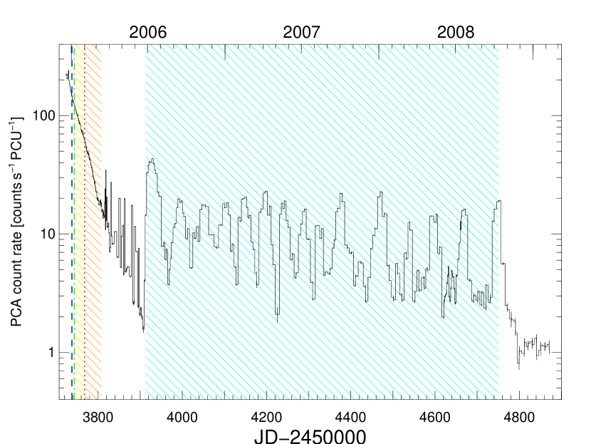
Figure 1.— PCA light curve of Swift J1626.6$-$5156, taken from HEASARC’s RXTE mission-long data archive (ftp://legacy.gsfc.nasa.gov/xte/data/archive/MissionLongData). It shows the background subtracted 2–20 keV count rate as recorded in standard2 mode (16 s time resolution), averaged over each observation and normalized to a single PCU. The three vertical lines indicate when the longest observations were taken in January 2006. LO1 is the blue dashed line, LO2 the green dot-dashed line, and LO3 the red dotted line. The shaded regions represent the Data Sections, with DS1 in yellow, DS2 in orange, and DS3 in teal.

Table 1Observation Log

Name	Observation ID	Date	$\mathrm{JD}-2450000$	PCA $t_{\mathrm{exp}}$	HEXTE $t_{\mathrm{exp}}$ [ks]
LO1	91081-13-01	2006 Jan 1	3736.05	26.4	8.4
LO2	91081-13-02	2006 Jan 6	3741.15	23.6	7.4
DS1	91082-01-01 – 91082-01-27	2006 Jan 12–30	3747.73–3765.10	23.3	7.1
LO3	91081-13-04	2006 Jan 31	3766.59	27.6	7.7
DS2	91082-01-32 – 91082-01-93	2006 Feb 1–Mar 13	3767.64–3807.52	51.2	–
DS3	92412-01-27 – 93402-01-48	2006 Jun 26–2008 Oct 10	3912.21–4750.82	78.8	–

Swift J1626.6$-$5156 was discovered during a Type II outburst, which is thought to occur when the Be star’s circumstellar disk expands and temporarily engulfs the neutron star, leading to enhanced accretion and therefore a large increase in X-ray emission (Coe, 2000, and references therein). Reig et al. (2008) describe the exponential decay of the outburst and the flaring behavior that occurred in the weeks immediately following the discovery. Additional flaring occurred following JD 2453800 (2006 March 5), after which the source transitioned into an epoch of long-term, quasi-periodic X-ray oscillations (Reig et al., 2008). A Lomb-Scargle periodogram (Lomb, 1976; Scargle, 1982) of the light curve first revealed an oscillation period from $\sim$JD 2454000–JD 2454350 (2006 September–2007 September) of $\sim$47 days and from $\sim$JD 2454350–2454790 (2007 September–2008 November) of $\sim$3/2 of this, or $\sim$72.5 days (DeCesar et al., 2009). Recent work by Baykal et al. 2010 found the long-term variability timescale to range from $\sim$45 to 95 days. Additionally, from pulse timing analysis, they find the binary orbit to be nearly circular (eccentricity 0.08) with a period of 132.9 days, meaning the oscillations occur on timescales of $\sim$1/2 and $\sim$2/3 of the orbital period. The oscillations therefore cannot be explained by bursts of accretion during periastron passages. On JD 2454791 (2008 November 11) the oscillatory behavior ceased and the 2–20 keV PCA count rate from Swift J1626.6$-$5156 dropped to $\sim$$1\,\mathrm{count}\,\mathrm{s}^{-1}\,\mathrm{PCU}^{-1}$.

Many BeX and other HMXB systems harbor neutron stars with very strong magnetic fields, typical strengths being $\sim 10^{11-13}$ G, and some of these systems exhibit cyclotron resonance scattering features (CRSFs or cyclotron lines). Observing cyclotron lines in the spectra of these systems is the only direct way to measure the magnetic field strengths of neutron stars. At the time of writing there are sixteen neutron star X-ray binaries with confirmed CRSFs (Heindl et al., 2004; Caballero & Wilms, 2012; Pottschmidt et al. 2012, , and references therein), eight of which are transients (Swift J1626.6$-$5156 being the ninth). Of the transients four systems are BeX binaries (Swift J1626.6$-$5156 being the fifth) and four are OeX binaries. The persistent sources are HMXBs with an O- or B-star accompanying the neutron star (with exception of Her X-1 and 4U 1626$-$67, where the companion is of lower mass). The fundamental cyclotron line energy is related to the magnetic field strength of the neutron star $E_{\mathrm{cyc}}\sim 11.6\,B_{12}(1+z)^{-1}$ keV where $B_{12}=B/10^{12}\,\mathrm{G}$ and $z$ is the surface gravitational redshift. Assuming a reasonable value of $z=0.3$, corresponding to a typical neutron star mass of $1.4M_{\odot}$, allows the direct calculation of $B$ in the region local to the magnetic pole where the cyclotron lines are produced.

In this Paper we discuss the discovery of a CRSF in the spectrum of Swift J1626.6$-$5156. In §2 we describe our data reduction and analysis techniques. §3 presents results from modeling the broad band X-ray spectra, including CRSFs and other spectral properties of the source. We summarize our findings and compare Swift J1626.6$-$5156 with other cyclotron line sources in §4 and conclude in §5.

2. Observations and Data Analysis

For this analysis, we considered data from the Proportional Counter Array (PCA; Jahoda et al., 2006) and the High Energy X-ray Timing Experiment (HEXTE; Rothschild et al., 1998) onboard RXTE that were taken between December 2005 and April 2009. From HEXTE, we used spectra from only the B cluster, since the A cluster had stopped rocking at the time of these observations, i.e., no background measurements for cluster A were available anymore. We extracted spectra in standard2 mode from the top layer of each PCA Proportional Counter Unit (PCU) separately. We then combined all spectra from a given observation into one, following the recipe in the RXTE Cookbook and excluding data taken within 10 min of the South Atlantic Anomaly. For a more detailed description of the data reduction and screening procedure see Wilms et al. (2006). We considered the PCA energy range 4–22 keV and the HEXTE range 18–60 keV when modeling the phase averaged spectra.

Three long observations with PCA exposure time $>$20 ks are available in the RXTE archive, along with hundreds of shorter monitoring observations. We combined the individual pointings of each observation as described in the RXTE Cookbook. The three “Long Observations”, which we refer to as LO1, LO2, and LO3, were each analyzed separately, while the data between and beyond these observations were combined into “Data Sections”, referred to as DS1, DS2, and DS3. Data prior to LO1 were excluded in order to avoid spectral contamination from flaring events (for a description of the flares, see Reig et al., 2008). For DS3 we combined only observations from the oscillating phase that had an average PCA 2–20 keV count rate of 10 $\mathrm{counts}\,\mathrm{s}^{-1}\,\mathrm{PCU}^{-1}$ or higher. The observation identification numbers and other information are given in Table 1. The locations in time of LO1–3 are shown by the colored lines and of DS1–3 by the shaded regions in Figure 1. The HEXTE data have low count rates, so we rebinned the counts at high energies using the FTOOL grppha. For LO1 and LO2 we rebinned by three energy channels above 50 keV and for LO3 by four channels above 48 keV. We did not rebin any counts for DS1. The HEXTE data of DS2 and DS3 were so noisy we decided not to use them as they might skew our spectral fits. We used xspec12 models (Arnaud, 1996; Dorman & Arnaud, 2001) for all spectral fitting.

3. Spectral Analysis

3.1. Spectral Model

We modeled the combined PCA and HEXTE (where present) phase averaged spectra of each LO and DS with a power law modified by a smooth exponential rollover (cutoffpl in xspec) including photoelectric absorption (phabs in xspec) and a Gaussian 6.4 keV Fe K$\alpha$ emission line (gauss in xspec):

$$I_{\mathrm{cont+Fe}}(E) = e^{-N_{\mathrm{H}}\sigma_{\mathrm{bf}}(E)}\left\{A_{\mathrm{cut}}E^{-\Gamma}e^{-\frac{E}{E_{\mathrm{fold}}}}\right.$$ (1)

$$+\left.\frac{A_{\mathrm{Fe}}}{\sigma_{\mathrm{Fe}}\sqrt{2\pi}}e^{-\frac{1}{2}[(E-E_{\mathrm{Fe}})^{2}/\sigma_{\mathrm{Fe}}^{2}]}\right\}$$

where $N_{\mathrm{H}}$ and $\sigma_{\mathrm{bf}}$ are the absorption model components and are respectively the hydrogen column density per H atom for material of cosmic abundance ($\mathrm{atoms}\,\mathrm{cm}^{-2}$) and the bound-free photoelectric absorption cross section ($\mathrm{cm}^{2}$). We used the abundances of Anders & Grevesse (1989) and the cross sections of Bałucińska-Church & McCammon (1992).

The first term in Eq. 1 is the cutoff power law, where $A_{\mathrm{cut}}$ is the power law normalization ($\mathrm{photons}\,\mathrm{keV}^{-1}\,\mathrm{cm}^{-2}\,\mathrm{s}^{-1}$ at 1 keV), $\Gamma$ is the power law photon index, and $E_{\mathrm{fold}}$ is the e-folding energy of the exponential rollover. The second term is the Gaussian emission line, in which $A_{\mathrm{Fe}}$ is its normalization ($\mathrm{photons}\,\mathrm{cm}^{-2}\,\mathrm{s}^{-1}$), $E_{\mathrm{Fe}}$ its energy, and $\sigma_{\mathrm{Fe}}$ its width. This model was applied concurrently to the PCA and HEXTE data, differing only by a constant flux cross-calibration factor where the constant was fixed at 1 for the PCA and fit to $\sim$0.8 for HEXTE. For each spectral fit we also fit the background strength adjusting it on a level of $\sim$0.1% using the command recornorm in xspec.

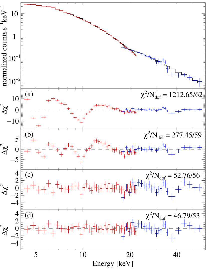
Figure 2.— The $\sim$4–60 keV spectrum and best-fit model for observation LO3 are shown in the main panel. PCA data are shown in red, HEXTE data in blue. a) The $\Delta\chi^{2}$ residuals left from fitting the spectrum with a cutoff power law. The spectrum peaks near $6.4\,$keV and dips near $10\,$keV. b) Residuals from adding a Gaussian emission line at $\sim 6.4\,$keV to the cutoff power law, completing our continuum plus Fe line fit from Equation 1. The depression at $10$ keV remains. c) Including a Gaussian optical depth absorption line near $10$ keV removes the absorption-like feature and greatly improves the model, giving our best fit (Equation 2). There may be a second feature near $18$ keV. d) A second Gaussian optical depth absorption feature included near $18$ keV marginally improves the fit. The remaining residual near $\sim 36$ keV is most likely caused by an instrumental effect (§3.2.7).

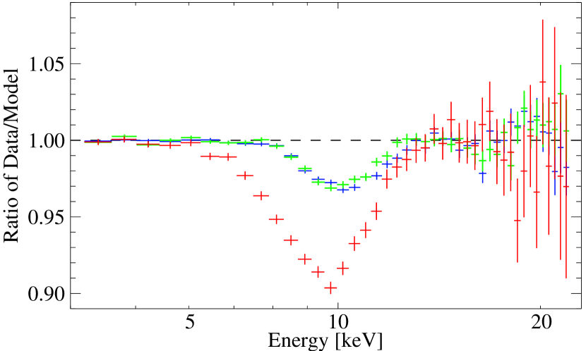
Figure 3.— Removing the Gaussian optical depth absorption component in our spectral model reveals the profile of the fundamental cyclotron line at $\sim$10 keV in LO1 (blue), LO2 (green), and LO3 (red). A decrease of the central energy between LO1–LO2 (close in time) and LO3 is apparent, as well as an increase in line depth.

Residuals for a continuum fit using the model from Eq. 1 without and with the iron emission line for LO3 are shown in Figs 2a and 2b, respectively. A depression in the residuals at $\sim$10 keV is apparent. In order to account for this feature, we modified the continuum plus Fe line model with a multiplicative absorption-like cyclotron line with a Gaussian optical depth profile (gabs in xspec):

$$I(E)=I_{\mathrm{cont+Fe}}(E)\exp\left\{\frac{-\tau_{\mathrm{cyc}}}{\sigma_{\mathrm{cyc}}\sqrt{2\pi}}\exp\left[-\frac{(E-E_{\mathrm{cyc}})^{2}}{2\sigma_{\mathrm{cyc}}^{2}}\right]\right\}$$ (2)

Here $\tau_{\mathrm{cyc}}$, $\sigma_{\mathrm{cyc}}$, and $E_{\mathrm{cyc}}$ are respectively the optical depth, line width, and line energy of the cyclotron line. The residuals of a fit to LO3 using the full model $I(E)$ of Eq. 2, i.e., including the cyclotron line, are displayed in Figure 2c.

In the following sections we describe the modeling and interpretation of this line as a CRSF including several tests that led to the adoption of the model described above as the best-fit model for the phase averaged spectra (constant$\times$phabs$\times$(cutoffpl + gauss)$\times$gabs in xspec).

Table 2Spectral parameters for phase averaged spectra

Name	$N_{\mathrm{H}}$	$\Gamma$	$A_{\mathrm{cut}}$	$E_{\mathrm{fold}}$	$E_{\mathrm{Fe}}$	$\sigma_{\mathrm{Fe}}$	$A_{\mathrm{Fe}}$	$E_{\mathrm{cyc}}$	$\sigma_{\mathrm{cyc}}$	$\tau_{\mathrm{cyc}}$	$F$	$\chi^{2}/N_{\mathrm{dof}}$
	[$10^{22}$]b		[$10^{-1}$]c	[keV]	[keV]	[keV]	[$10^{-3}$]d	[keV]	[keV]		[$10^{-10}\,\mathrm{cgs}$]
LO1	$4.8^{+0.6}_{-0.6}$	$1.11^{+0.04}_{-0.05}$	$2.8^{+0.2}_{-0.3}$	$10.46^{+0.33}_{-0.34}$	$6.33^{+0.03}_{-0.04}$	$0.49^{+0.05}_{-0.05}$	$3.3^{+0.5}_{-0.4}$	$10.23^{+0.09}_{-0.09}$	$0.99^{+0.17}_{-0.17}$	$0.097^{+0.025}_{-0.021}$	$19.10^{+0.02}_{-0.10}$	$81.9/68$
LO2	$4.5^{+0.8}_{-0.7}$	$1.20^{+0.06}_{-0.05}$	$2.5^{+0.3}_{-0.2}$	$11.50^{+0.52}_{-0.39}$	$6.30^{+0.04}_{-0.04}$	$0.54^{+0.07}_{-0.05}$	$3.0^{+0.4}_{-0.5}$	$10.01^{+0.09}_{-0.08}$	$0.76^{+0.15}_{-0.16}$	$0.082^{+0.020}_{-0.017}$	$16.80^{+0.03}_{-0.20}$	$78.9/68$
DS1	$4.8^{+0.8}_{-0.7}$	$1.37^{+0.07}_{-0.06}$	$2.4^{+0.3}_{-0.3}$	$12.72^{+0.79}_{-0.37}$	$6.34^{+0.05}_{-0.04}$	$0.45^{+0.06}_{-0.08}$	$1.7^{+0.3}_{-0.3}$	$9.74^{+0.07}_{-0.07}$	$0.96^{+0.13}_{-0.12}$	$0.15^{+0.02}_{-0.02}$	$11.80^{+0.04}_{-0.20}$	$94.1/76$
LO3	$3.4^{+0.7}_{-0.8}$	$1.32^{+0.09}_{-0.09}$	$1.7^{+0.2}_{-0.2}$	$10.98^{+0.97}_{-0.91}$	$6.38^{+0.04}_{-0.04}$	$0.19^{+0.10}_{-0.18}$	$0.9^{+0.2}_{-0.1}$	$9.71^{+0.07}_{-0.07}$	$1.27^{+0.16}_{-0.15}$	$0.33^{+0.04}_{-0.06}$	$8.62^{+0.04}_{-0.19}$	$52.8/56$
DS2	$1.4^{+0.8}_{-1.2}$	$1.61^{+0.07}_{-0.08}$	$1.0^{+0.1}_{-0.1}$	$19.07^{+1.83}_{-2.47}$	$6.36^{+0.03}_{-0.06}$	$0.41^{+0.05}_{-0.06}$	$0.8^{+0.2}_{-0.1}$	$10.00^{+0.08}_{-0.08}$	$0.64^{+0.02}_{-0.02}$	$0.25^{+0.04}_{-0.04}$	$4.44^{+0.03}_{-0.15}$	$59.4/33$
DS3a	–	$1.37^{+0.07}_{-0.07}$	$0.33^{+0.02}_{-0.02}$	$13.20^{+1.67}_{-1.30}$	$6.48^{+0.02}_{-0.02}$	$0.41^{+0.05}_{-0.06}$	$0.40^{+0.04}_{-0.04}$	$9.44^{+0.07}_{-0.06}$	$0.64^{+0.11}_{-0.12}$	$0.25^{+0.04}_{-0.04}$	$2.06^{+0.003}_{-0.04}$	$52.4/32$

Note. — The best-fit spectral parameters from each observation or group of observations. $N_{\mathrm{H}}$ is the column density, $\Gamma$ the power law photon index, $A_{\mathrm{cut}}$ the power law normalization, $E_{\mathrm{fold}}$ the folding energy of the cutoff power law, $E_{\mathrm{Fe}}$, $\sigma_{\mathrm{Fe}}$, and $A_{\mathrm{Fe}}$ the iron emission line energy, width, and normalization, $E_{\mathrm{cyc}}$, $\sigma_{\mathrm{cyc}}$, and $\tau_{\mathrm{cyc}}$ the energy, width, and optical depth of the Gaussian optical depth absorption line profile used to fit the cyclotron line, $F$ the 3–20 keV source flux in units of $10^{-10}\,\mathrm{erg}\,\mathrm{cm}^{-2}\,\mathrm{s}^{-1}$, and $\chi^{2}/N_{\mathrm{dof}}$ the reduced $\chi^{2}$ (where $N_{\mathrm{dof}}$ is the number of degrees of freedom), of each spectral fit. The changing $N_{\mathrm{dof}}$ results from differences in rebinning of the HEXTE data (see §2) for the LO1–LO3 columns, and from our choice to not use HEXTE data for DS2–3. The error bars quoted are at the 90% level. The 90% flux errors were calculated in xspec using 1000 draws from a Gaussian distribution. ^aDS3 requires an additional Gaussian emission component with energy $15.18^{+0.17}_{-0.17}$ keV, $\sigma$ fixed at 0.30 keV, and normalization $7.3^{+1.4}_{-1.4}\times 10^{-5}\,\mathrm{photons}\,\mathrm{cm}^{-2}\,\mathrm{s}^{-1}$. ^bValues of $N_{\mathrm{H}}$ are in units of $10^{22}\,\mathrm{atoms}\,\mathrm{cm}^{-2}$. ^cUnits are $10^{-1}\,\mathrm{photons}\,\mathrm{keV}^{-1}\,\mathrm{cm}^{-2}\,\mathrm{s}^{-1}$ at 1 keV. ^dValues are given in units of $10^{-3}\,\mathrm{photons}\,\mathrm{cm}^{-2}\,\mathrm{s}^{-1}$.

3.2. Pulse phase averaged spectra

3.2.1 Best-fit results, 10 keV CRSF detection

We used LO3, the longest observation of Swift J1626.6$-$5156, to illustrate the results obtained with the best-fit model described in the previous section. This observation was taken on 2006 January 31, during the outburst decay (Figure 1). The first PCA pointing is $\sim$21 ks long and is followed immediately by a shorter pointing of $\sim$6 ks. We combined them to form a single spectrum with PCA integration time $\sim$27 ks. The corresponding HEXTE observation has $\sim$7.6 ks of live time. The best-fit parameters for the LO3 spectrum using the model of Eq. 2, along with the iron line equivalent width and other characteristics, can be found in the fourth row of Table 2. The phase averaged spectrum of LO3 and best-fit model are shown in the main panel of Figure 2. Inspecting the residuals obtained after fitting the continuum model and iron line (Equation 1) shown in Figure 2b more closely reveals the absorption-like feature near 10 keV and/or an emission-like feature near 14 keV. Here we treated the feature as absorption-like only (Equation 2) and obtained a very good fit. See §3.2.2–3.2.5 for testing possible alternative descriptions. Fitting the feature with a Gaussian optical depth absorption line flattened the residuals in Figure 2c, yielding $\chi^{2}_{\mathrm{red}}=0.94$ for 56 degrees of freedom. The common $\Delta\chi^{2}$ test available in xspec could not be applied in this case, as it is not applicable to multiplicative model components (Orlandini et al., 2012). We instead used the more appropriate ratio of variances $F$-test (Press et al., 2007) to calculate the probability that including this absorption-like feature in the model improves the fit by chance. As discussed by Orlandini et al. (2012), this $F$-test is not available in xspec; throughout this paper, we use the IDL routine mpftest to calculate the probability of chance improvement (PCI) from one model to another. If one model is not a significant improvement over another, then the PCI will be large. The PCI of the model that includes the Gaussian-depth absorption feature (Figure 2c) compared to that without (Figure 2b) is $4.6\times 10^{-9}$. The improvement to the fit due to use of the absorption-like model component is therefore very statistically significant. The best-fit parameters of this model are given in Table 2.

The CRSF is detected in the earlier two long outburst observations, LO1 and LO2, as well. Figure 3 shows the line profiles for LO1–LO3. We also detected a strong iron line in each of the spectra. See Table 2 for the best-fit results. One question we may ask is whether or not the cyclotron line persists throughout and beyond the primary outburst decay. To answer this we combined sections of data into single spectra to search for the line. The data selection is described in §2 and summarized in Table 1. We found that both the iron line and the CRSF were present throughout the active phase of Swift J1626.6$-$5156, as the features are detected in each of the Data Sections DS1–DS3 as well as in the Long Observations. Interestingly, we found that the spectrum from the oscillatory stage of the light curve (DS3) is best fit by the addition of a Gaussian emission line at $\sim$15 keV, a component that was not necessary in any of the spectra taken during the outburst decay (see §3.2.5) but that is commonly used to fit HMXB spectra (Coburn et al., 2002). All fit parameters are given in Table 2. The values of $E_{\mathrm{cyc}}$ are suggestive of an evolution of the cyclotron line energy with luminosity, which is discussed in §4.3. Note that the parameters might be affected by additional uncertainties due to the range of fluxes covered for DS1–DS3 and missing HEXTE data for DS2–DS3, though.

“Bumps” or “wiggles” in the spectra of accreting X-ray pulsars, especially near 10 keV, are common and have been discussed at some length by Coburn et al. (2002). They find residuals in the data/model ratio at the $\sim$0.8% level in all the accreting systems they examine. These residuals could easily be interpreted as cyclotron features. There have been marginal detections of absorption-like features, possibly cyclotron lines, near 10 keV in other sources. One example is the recent work on XMMU J054134.7$-$682550 (catalog ) by İnam et al. (2009). These authors see what may be an absorption-like feature at 10 keV, but the count rate is too low to claim a significant detection. One must thus take good care to ensure that the feature we see is truly a cyclotron line and not due to calibration uncertainties, additional emission (e.g., from the Galactic ridge), or incorrect modeling of the continuum. We note that the residuals we see at $\sim$10 keV are on the 3–10% level (Figure 3), i.e., comparatively strong. Nevertheless we address these potential sources of uncertainties in §3.2.2, §3.2.3, and §3.2.4–§3.2.5, respectively. We also note that Reig et al. (2011) state that they do not detect a cyclotron line in the RXTE outburst data. However, these authors include a 9 keV edge in their model apparently masking the CRSF. This model choice misses the typical CRSF properties of the observed residual that we present in this paper (e.g., its luminosity or pulse phase dependence).

3.2.2 Crab spectrum comparison

Figure 4.— Ratio of Swift J1626$-$5156 (observation LO3) to Crab counts according to the procedure described by Orlandini et al. (1998). The depression at $\sim$10 keV is present in this model- and calibration-independent representation of the spectrum of Swift J1626$-$5156 as well.

One test we can perform in order to validate the existence of the cyclotron line in the phase averaged spectrum is to compare the spectrum of Swift J1626.6$-$5156 with that of a non-cyclotron line source like the Crab pulsar. To be as consistent as possible in our comparison, we used Swift J1626.6$-$5156 and Crab data only from PCU 2, which is the best calibrated of the five PCUs (Jahoda et al., 2006) and which is most often turned on during observations. The Crab data included both the pulsar and the nebula, and were taken between November 2005 and March 2006, the same time period during which the Swift J1626.6$-$5156 observations LO1–3 were taken.

We first searched for an absorption-like feature near 10 keV in the Crab spectral residuals. The Crab has no CRSFs, so if such a feature were seen in the Crab spectrum, we could assume that the Swift J1626.6$-$5156 feature was instrumental in origin. We modeled the Crab spectrum with an absorbed power law, freezing $N_{\mathrm{H}}$ at $4\times 10^{21}\,\mathrm{cm}^{-2}$, the value determined for the Crab by Weisskopf et al. (2004). The power law parameters were left free, and we found that $\Gamma=2.095$ with a normalization of 10.343 $\mathrm{photons}\,\mathrm{keV}^{-1}\,\mathrm{cm}^{-2}\,\mathrm{s}^{-1}$ at 1 keV gave the best fit. The data/model ratio is $\sim$0.99 near 10 keV, which is consistent with expected calibration uncertainties (Jahoda et al., 2006). No absorption-like feature is found at 10 keV in the Crab spectrum (and no rollover). We repeated the procedure with PCU 2 data from Swift J1626.6$-$5156 during LO3, using a cutoff power law and fixing $N_{\mathrm{H}}$ and $\Gamma$ to the values in Table 2. In this case the ratio near 10 keV is $\sim$0.91, a much larger residual than consistent with calibration errors.

Table 3Comparison with alternative continuum models

Continuum Model	$E_{\mathrm{Fe}}$	$E_{\mathrm{cyc}}$	$\chi^{2}_{\mathrm{red}}$	$N_{\mathrm{dof}}$	PCI
	[keV]	[keV]
cutoffpl	$6.38^{+0.04}_{-0.04}$	$9.71^{+0.07}_{-0.07}$	$0.94$	$56$	–
power$\times$highecut	$6.38^{+0.04}_{-0.04}$	$9.74^{+0.08}_{-0.07}$	$0.96$	$55$	$0.47$
power$\times$fdcut	$6.38^{+0.04}_{-0.04}$	$9.79^{+0.11}_{-0.12}$	$1.12$	$55$	$0.26$
npex	$6.38^{+0.06}_{-0.06}$	$9.83^{+0.28}_{-0.25}$	$1.02$	$54$	$0.38$

Note. — Comparison between the cutoffpl continuum model with the highecut, fdcut, and npex models described in §3.2.4. All spectral modeling was performed on the LO3 dataset. Fits with the alternative continuum models yield values of $E_{\mathrm{Fe}}$ and $E_{\mathrm{cyc}}$, defined as in Table 2, that are consistent with the line energies found using the cutoffpl model. The probability of chance improvement (PCI) is described in §3.2.4 and calculated with $\chi^{2}_{\mathrm{red}}$ and $N_{\mathrm{dof}}$ of the cutoffpl and each of the alternative models. The PCI is large for each of the three alternative models, meaning that the different continuum models are statistically equivalent. For ease of comparison, we repeat the selected results for the cutoffpl continuum from Table 2.

We next took a model and calibration independent approach by comparing the raw counts of Swift J1626.6$-$5156 with those of the Crab in each spectral energy bin following the procedure of Orlandini et al. (1998). We first subtracted the background counts from each raw spectrum, making sure to account for the difference in exposure time between the two sources. We then divided the Swift J1626.6$-$5156 count rates by those of the Crab, resulting in the ratio shown in Figure 4. At $\lesssim$6 keV the J1626/Crab ratio reflects the steeper slope of the Crab and at $\gtrsim$14 keV the missing Crab rollover. Between these energies an enhancement at 6.4 keV due to the iron line in Swift J1626.6$-$5156 and a clear depression at $\sim$10 keV, rather than a smooth transition between the iron line and the power law tail, are apparent. The same kind of Crab ratio is shown, e.g., for the $\sim$55 keV CRSF of Vela X-1 (catalog ) in the upper panel of Figure 3 of Orlandini et al. (1998). This plot shows similar cyclotron line and rollover features as the J1626/Crab ratio (it differs at lower energies due to the overall different energy range). Independently of the response function or spectral model the J1626/Crab ratio therefore supports that the absorption-like feature does not result from a calibration error.

3.2.3 Galactic ridge emission

We also investigated the possibility that cyclotron features in the spectrum arise from the Galactic ridge emission by analyzing data from when the source was quiescent. While Swift J1626.6$-$2126 remained fairly bright and highly variable for about 1000 days after the initial outburst, it then quickly faded to quiescence (Figure 1) and stayed reliably low for the last two years of the RXTE mission. During this time the source continued to be monitored regularly by the PCA. We combined these late observations to obtain a spectrum with a total of 42 ks exposure, and compared this with our outburst observations, in order to put limits on the contribution of the flux during the outburst observations from the underlying Galactic ridge emission. In the 10 keV region surrounding the fundamental cyclotron line, the ridge emission has a flux of less than 1% of the count rate of Swift 1626.6$-$5156 during our observations (LO3). In the energy range around the first harmonic ($\sim$18 keV, see §3.2.6 and §3.3) no emission from the ridge is detected. Therefore Galactic ridge emission cannot explain the deviations that we measure.

3.2.4 Alternative standard continuum and CRSF models

In order to test the continuum model dependence of our results we in turn replaced the cutoff power law model by three other standard empirical pulsar continuum models and repeated the fit for LO3. The first of these was the power law with a high energy cutoff (power$\times$highecut in xspec where, in contrast to the smooth cutoff power law, the rollover in the spectrum only starts at a certain energy, $E_{\mathrm{cut}}$ (White et al., 1983). While this model is often used, it can create an artificial line-like residual near $E_{\mathrm{cut}}$ due to the discontinuity at that energy (Coburn et al., 2002, and references therein). Next we fit the spectrum with the Fermi-Dirac cutoff from Tanaka (1986) (power$\times$fdcut in xspec). This model has a smooth, continuous rollover described by $E_{\mathrm{cut}}$ and $E_{\mathrm{fold}}$, which are, however, not directly comparable to the values obtained with cutoffpl or power$\times$highecut due to differences in the continua. The final model we used is the Negative Positive Exponential model from Mihara (1995) (npex in xspec), which consists of two power laws with a smooth exponential cutoff described by $E_{\mathrm{fold}}$. Each of these models was fit to LO3 modified by absorption and with the added 6.4 keV Gaussian emission line and cyclotron line. The fit values of the Gaussian emission line and the CRSF energy found for each model are given in Table 3.

These alternative continuum models were found to produce fits of similar quality when compared with each other and with the cutoffpl model. They also produced identical results, within errors, for all comparable parameters, most notably those of the 10 keV CRSF. The $\Delta\chi^{2}$ test cannot be used to compare different continuum models (Protassov et al., 2002; Orlandini et al., 2012). To quantify whether or not the cutoffpl model, which has the lowest $\chi^{2}_{\mathrm{red}}$ of the four continuum models tested, actually improves the continuum fit when compared to the alternative models, we calculated the PCI (as in §3.2.1) of the cutoffpl model. Orlandini et al. (2012) discuss the appropriateness of this $F$-test for comparison between different models, and the statistic is applied in this way by Iwakiri et al. (2012). Table 3 gives the reduced $\chi^{2}_{\mathrm{red}}$, number of degrees of freedom, and PCI (compared to cutoffpl) for each alternative model. We find that the PCI is between $\sim$25–50%, meaning that the cutoffpl improves the continuum fit marginally at best. Because none of the canonical models clearly gave a best fit to the continuum, nor adjusted the energies of the 6.4 keV line or the 10 keV feature, and since cutoffpl has the smallest number of parameters, we defaulted to this model, our original choice, as a result of this test. The cutoffpl model is also well suited for comparisons with many earlier results for similar sources (Coburn et al., 2002; Mowlavi et al., 2006; Caballero et al., 2008; Suchy et al., 2011).

Also, in order to further check that the $10\,$keV feature is robustly described as a typical CRSF, we compared the Gaussian optical depth absorption model with a Lorentzian profile model (cyclabs in xspec) (Mihara, 1990). Taking the known systematic shift into account we found similar centroid energies for the absorption-like feature using either model. We chose to use gabs in our analysis because its parametrization provides an easier to interpret and compare characteristic energy parameter (in contrast to gabs the energy parameter of cyclabs does not directly reflect the energy where the absorption-like feature in the spectrum is deepest).

3.2.5 Modified continuum models

Many accreting pulsar spectra are either not adequately or at least not uniquely described by the standard empirical continuum models above, especially in the 10–20 keV range (Coburn et al., 2002; Orlandini, 2004). Incorrect modeling of the exact shape of the rollover can create residuals in addition to CRSF features or, in the worst case, mimic CRSFs. There are many examples for the application of continuum models with slightly modified cutoff characterization. Orlandini et al. (1999) noted the likely presence of a two step change of the spectral slope for OAO 1657$-$415 (catalog ) (as well as a potential cyclotron line residual near 36 keV), the first change occurring at 10–20 keV and the other one at higher energies, however, they were able to model this behavior taking advantage of the discontinuity and the two characteristic energies of the highecut model mentioned above. Other authors used an additional polynomial component in order to describe a more complex rollover shape, i.e., Burderi et al. (2000) for Cen X-3 (catalog ) (an established cyclotron line source) and Klochkov et al. (2008) for EXO 2030$+$375 (catalog ) (noting a potential cyclotron line residual near 63 keV). The correct continuum and therefore the presence of a 25 keV CRSF in Vela X-1 (catalog ) (in addition to the established $\sim$55 keV one) has long been debated (Orlandini et al., 1998; Kreykenbohm et al., 2002; La Barbera et al., 2003). In the most recent analysis its presence was confirmed in a Suzaku observation (Doroshenko et al., 2011). Another widely used modification is obtained by adding a broad Gaussian component, most often in emission, to a standard or already modified model (Coburn et al., 2002; Klochkov et al., 2007, 2008; Ferrigno et al., 2009; Suchy et al., 2008, 2011). Since our Swift J1626.6$-$5156 observations show a positive residual at $\sim$14 keV before modeling the cyclotron line (Figure 2b) we applied this modified model to test whether our cyclotron line detection is robust against the choice of a more complex rollover description.

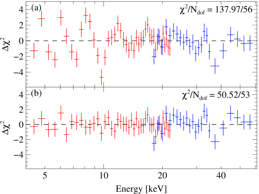
Figure 5.— a) Starting from the continuum plus Fe line fit (Equation 1) for observation LO3 (residuals shown in Figure 2b), we further smoothed the continuum in this alternative fit by first including a broad Gaussian emission feature centered at 13.7 keV. While this flattens the residuals substantially, the absorption-like feature at 10 keV still remains. b) Final fit for this mixed emission/absorption approach after also including the 9.7 keV cyclotron line. The remaining residual near $\sim 36$ keV is most likely caused by an instrumental effect (§3.2.7).

We therefore altered our fit procedure by first adding a broad emission line near $14\,$keV to the initial continuum plus Fe line fit for LO3 (Figure 2b, Equation 1). The residuals of this fit are shown in Figure 5a. The negative residual near 10 keV is still clearly visible, giving a $\chi^{2}_{\mathrm{red}}$ of 2.46 for 56 dof. Thus an absorption-like feature was still required for an adequate description. Multiplying by a Gaussian optical depth absorption feature and refitting we obtained $E_{\mathrm{cyc}}=9.74^{+0.16}_{-0.12}$ keV, $\sigma_{\mathrm{cyc}}=0.93^{+0.22}_{-0.28}$ keV, $\tau_{\mathrm{cyc}}=0.14^{+0.04}_{-0.07}$ for the cyclotron line and $E_{\mathrm{em}}=13.8^{+0.7}_{-1.6}$ keV, $\sigma_{\mathrm{em}}=1.86^{+0.98}_{-0.67}$ keV, $A_{\mathrm{em}}=0.26^{+0.33}_{-0.15}10^{-3}$ photons cm^-2 s^-1 for the emission-like line. This fit with both lines yielded $\chi^{2}/N_{\mathrm{dof}}=49.96/53$ $(=0.94)$ (Figure 5b), as opposed to $52.76/56$ $(=0.94)$ for the original best-fit (Figure 2c, Table 2). The fits are equally good (PCI $=$ 50%). While the depth of the cyclotron line was smaller in the modified fit, the line was still detected at the same energy as before (Table 2). The parameters of the modified fit characterizing the continuum shape were $\Gamma=1.47^{+0.09}_{-0.11}$ and $E_{\mathrm{fold}}=12.58^{+1.26}_{-1.32}$ keV, consistent within errors with the original fit (Table 2). The same Fe line parameters were obtained for both fit procedures.

This implies that, while the underlying continuum might be slightly different from a standard cutoff power law, such a difference cannot be significantly detected in this observation. The absorption-like feature at 10 keV on the other hand is significant. It appears at 9.7 keV regardless of the presence or absence of a broad emission feature and its energy is stable. Based on these results and since the model without the broad emission feature is the simpler one, it is the one we chose as our best-fit model. The same overall behavior has been seen for all the datasets with the exception of DS3, for which a better fit was obtained including a broad emission feature, see notes of Table 2 for further details. This can be understood since the DS3 spectrum was obtained averaging over many datasets, which might contain some evolution of the continuum.

3.2.6 18 keV harmonic

Returning to Figure 2c we point out a small depression near 18 keV. In Figure 2d we show the obtained residuals after fitting this feature with another Gaussian optical depth absorption line with centroid energy $18.5^{+0.9}_{-0.6}$ keV, $\tau\sim 0.1^{+0.09}_{-0.07}$, and $\sigma$, which could not be constrained, fixed at $\sim$0.02. This additional component reduced $\chi^{2}$ slightly but did not significantly improve the fit, as its PCI $\sim$ 40% from the ratio of variances $F$-test (Press et al., 2007). We therefore did not include this feature in our best-fit model of the phase averaged spectrum, i.e., Table 2. While we would not normally consider this a detection, we also found that the addition of this 18 keV feature greatly improved the pulse phase resolved spectral fits (§3.3) during the pulse peak. It is marginally present in the phase averaged spectrum of LO2 as well. It is thus likely the first harmonic of the fundamental CRSF, which is significantly detected in only a few profile phase bins (see §3.3).

3.2.7 36 keV instrumental feature

Even after fitting the harmonic feature there remained an even more obvious line-like residual near 36 keV (Figures 2d and 5b). It is tempting to interpret this as a further harmonic. There might even be another weak residual at $\lesssim$30 keV. However, the effective area of HEXTE shows a sharp drop at 33 keV due to the K-edge of iodine with a smooth recovery until about 45 keV(see Figure 5 of Rothschild et al., 1998). So there is a good chance that (at least part of) any residuals in this energy range (is) are due to imperfect calibration (Heindl et al., 1999a). In addition the strongest internal HEXTE background line, which is due to K-lines from the tellurium daughters of various iodine decays, sits at 30 keV (Rothschild et al., 1998). We therefore decided to not further pursue the potential existence of harmonics beyond the first one at 18 keV. If Swift J1626.5$-$5156 shows other outbursts in the future the detection of these harmonics might be possible with higher sensitivity with Suzaku, or better, NuSTAR or Astro-H.

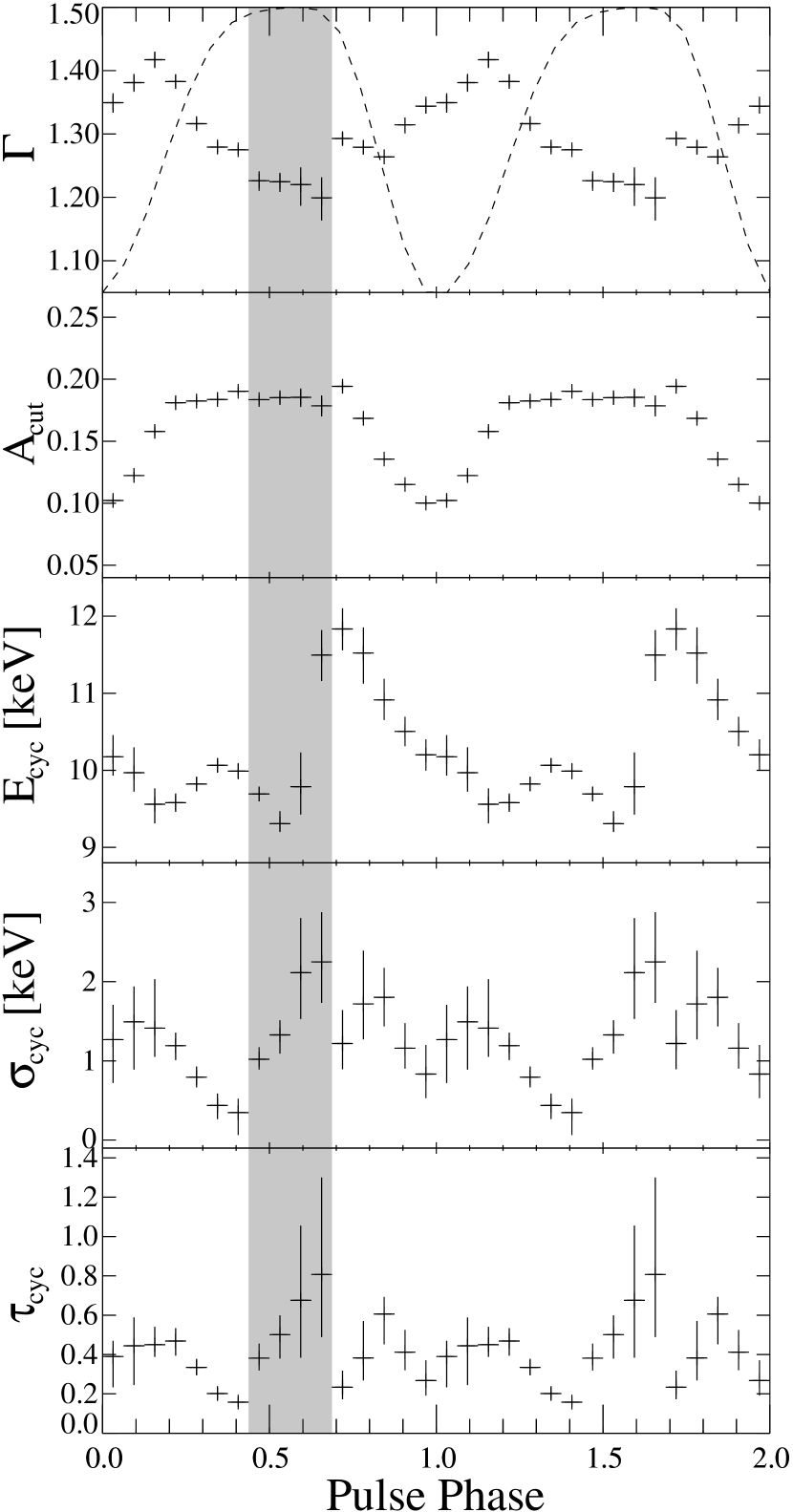
Figure 6.— Variability of the spectral parameters with phase for observation LO3. The top panel includes the 3.5–25 keV pulse profile of Swift J1626.6$-$5156 (dashed line) as well as the best-fit power law index (crosses). The shaded region indicates the four phase bins surrounding the pulse peak, in which a second CRSF line is necessary to produce an acceptable fit.

3.3. Pulse phase resolved spectra

We again used LO3, which shows the strongest cyclotron line, for a phase resolved spectral analysis. We extracted Good Xenon event data with a time resolution of 3.9 ms and corrected the event times to the Solar System barycenter. A period search on these data resulted in a pulse period of $15.35828\pm 0.00008$ s, consistent with the spin down evolution presented by Baykal et al. 2010 . We folded the 3.5–25 keV events on this period in order to obtain the pulse profile, see dashed line in the upper panel of Figure 6. As presented by Reig et al. (2008) the pulse profile shows a single broad peak with a roughly constant maximum over four phase bins. The falling edge seems to be steeper than the rising edge, which may be an artifact from the period folding. We did not include a binary correction since effects of the $\sim$133 d orbit (Baykal et al. 2010, ) are negligible for our $\lesssim$30 ks observation.

We divided the pulse profile into 16 phase bins for spectral analysis and used ikfasebin to extract spectra for each phase. Each spectrum was fit using Eq. 2 with an additional edge component at $\sim$5 keV to account for the Xenon L-edge calibration feature (Jahoda et al., 2006). Still we found it necessary to remove one spectral bin at $\sim$4.5 keV (spectral bin 12) from each phase’s spectrum to improve the overall fit. We assume that the systematic residual in this spectral bin is due to calibration uncertainties at lower energies and has no physical significance for the model. The column density and the iron emission energy were frozen at $3.4\times 10^{22}\,\mathrm{cm}^{-2}$ and 6.4 keV – the values from the phase averaged fit –, respectively. In order to better constrain the spectral index, the folding energy of the cutoff power law was also frozen at the phase averaged value of 10.98 keV.

Table 4Spectral parameters for phase resolved spectra from LO3

Phase	$\Gamma$	$A_{\mathrm{cut}}$	$\sigma_{\mathrm{Fe}}$	$A_{\mathrm{Fe}}$	$E_{\mathrm{cyc,1}}$	$\sigma_{\mathrm{cyc,1}}$	$\tau_{\mathrm{cyc,1}}$	$E_{\mathrm{cyc,2}}$	$\sigma_{\mathrm{cyc,2}}$	$\tau_{\mathrm{cyc,2}}$	$\chi^{2}_{\mathrm{red,2}}$	$\chi^{2}_{\mathrm{red,1}}$	$\chi^{2}_{\mathrm{red,0}}$	PCIc
Bin		[$10^{-1}$]a	[keV]	[$10^{-3}$]b	[keV]	[keV]		[keV]	[keV]		41 dof	43 dof	46 dof
$1$	$1.34^{+0.02}_{-0.01}$	$1.02^{+0.03}_{-0.03}$	$0.3^{+0.1}_{-0.3}$	$1.02^{+0.50}_{-0.34}$	$10.2^{+0.3}_{-0.2}$	$1.3^{+0.4}_{-0.5}$	$0.4^{+0.2}_{-0.1}$	$--$	$--$	$--$	$--$	1.34	$2.76$	$9.2\times 10^{-3}$
$2$	$1.38^{+0.02}_{-0.01}$	$1.22^{+0.03}_{-0.03}$	$0.3^{+0.2}_{-0.2}$	$1.15^{+0.75}_{-0.19}$	$10.0^{+0.3}_{-0.2}$	$1.6^{+0.5}_{-0.6}$	$0.5^{+0.1}_{-0.2}$	$--$	$--$	$--$	$--$	0.98	$2.10$	$6.5\times 10^{-3}$
$3$	$1.42^{+0.01}_{-0.01}$	$1.57^{+0.03}_{-0.03}$	$0.3^{+0.2}_{-0.3}$	$1.32^{+0.69}_{-0.38}$	$9.6^{+0.2}_{-0.1}$	$1.4^{+0.6}_{-0.4}$	$0.5^{+0.2}_{-0.1}$	$--$	$--$	$--$	$--$	0.93	$2.41$	$1.0\times 10^{-3}$
$4$	$1.38^{+0.01}_{-0.01}$	$1.81^{+0.04}_{-0.03}$	$0.0^{+0.0}_{-0.0}$	$1.10^{+0.29}_{-0.20}$	$9.6^{+0.1}_{-0.1}$	$1.2^{+0.2}_{-0.2}$	$0.5^{+0.0}_{-0.1}$	$--$	$--$	$--$	$--$	0.68	$4.64$	$1.8\times 10^{-9}$
$5$	$1.32^{+0.01}_{-0.01}$	$1.82^{+0.03}_{-0.03}$	$0.0^{+0.01}_{-0.00}$	$1.15^{+0.26}_{-0.24}$	$9.8^{+0.1}_{-0.1}$	$0.8^{+0.1}_{-0.1}$	$0.3^{+0.0}_{-0.0}$	$--$	$--$	$--$	$--$	0.96	$6.57$	$1.7\times 10^{-9}$
$6$	$1.28^{+0.01}_{-0.01}$	$1.83^{+0.04}_{-0.03}$	$0.8^{+0.1}_{-0.1}$	$2.75^{+0.52}_{-0.47}$	$10.0^{+0.2}_{-0.0}$	$0.4^{+0.2}_{-0.1}$	$0.2^{+0.0}_{-0.0}$	$--$	$--$	$--$	$--$	1.69	$5.46$	$8.6\times 10^{-9}$
$7$	$1.28^{+0.00}_{-0.01}$	$1.90^{+0.03}_{-0.03}$	$1.0^{+0.1}_{-0.2}$	$2.96^{+0.51}_{-0.46}$	$10.0^{+0.1}_{-0.1}$	$0.3^{+0.2}_{-0.3}$	$0.2^{+0.0}_{-0.1}$	$--$	$--$	$--$	$--$	1.41	$4.35$	$1.5\times 10^{-4}$
$8$	$1.23^{+0.01}_{-0.02}$	$1.84^{+0.03}_{-0.04}$	$0.0^{+0.4}_{-0.0}$	$0.62^{+0.26}_{-0.19}$	$9.7^{+0.1}_{-0.1}$	$1.0^{+0.2}_{-0.1}$	$0.4^{+0.1}_{-0.6}$	$17.5^{+0.6}_{-0.4}$	$2.5$	$0.8^{+0.2}_{-0.2}$	1.24	$2.29$	$5.38$	$2.5\times 10^{-2}$
$9$	$1.22^{+0.02}_{-0.01}$	$1.85^{+0.04}_{-0.04}$	$0.0^{+0.3}_{-0.0}$	$0.74^{+0.49}_{-0.20}$	$9.3^{+0.2}_{-0.1}$	$1.3^{+0.2}_{-0.2}$	$0.5^{+1.0}_{-0.1}$	$18.4^{+0.4}_{-0.4}$	$2.5$	$1.0^{+0.3}_{-0.2}$	1.05	$2.80$	$5.42$	$1.0\times 10^{-3}$
$10$	$1.22^{+0.03}_{-0.3}$	$1.85^{+0.07}_{-0.08}$	$0.4^{+0.1}_{-0.1}$	$2.28^{+1.14}_{-0.39}$	$9.8^{+0.4}_{-0.4}$	$2.1^{+0.7}_{-0.6}$	$0.7^{+0.4}_{-0.3}$	$18.7^{+0.3}_{-0.4}$	$2.5$	$1.3^{+0.5}_{-0.3}$	1.33	$2.81$	$3.64$	$8.8\times 10^{-3}$
$11$	$1.20^{+0.03}_{-0.03}$	$1.78^{+0.08}_{-0.08}$	$0.4^{+0.1}_{-0.0}$	$4.32^{+1.16}_{-1.02}$	$11.5^{+0.3}_{-0.3}$	$2.2^{+0.6}_{-0.5}$	$0.8^{+0.5}_{-0.3}$	$19.1^{+0.4}_{-0.5}$	$2.5$	$1.5^{+0.4}_{-0.5}$	1.17	$2.17$	$2.62$	$2.5\times 10^{-2}$
$12$	$1.29^{+0.01}_{-0.01}$	$1.94^{+0.03}_{-0.03}$	$0.4^{+0.1}_{-0.0}$	$4.40^{+0.68}_{-0.71}$	$11.8^{+0.3}_{-0.3}$	$1.2^{+0.4}_{-0.3}$	$0.2^{+0.1}_{-0.0}$	$--$	$--$	$--$	$--$	1.43	$2.58$	$2.7\times 10^{-2}$
$13$	$1.28^{+0.01}_{-0.01}$	$1.68^{+0.03}_{-0.03}$	$0.4^{+0.1}_{-0.1}$	$2.44^{+0.85}_{-0.69}$	$11.5^{+0.3}_{-0.4}$	$1.7^{+0.7}_{-0.4}$	$0.4^{+0.2}_{-0.1}$	$--$	$--$	$--$	$--$	0.89	$2.25$	$1.3\times 10^{-3}$
$14$	$1.26^{+0.01}_{-0.01}$	$1.35^{+0.03}_{-0.03}$	$0.3^{+0.1}_{-0.3}$	$1.13^{+0.71}_{-0.34}$	$10.9^{+0.3}_{-0.3}$	$1.8^{+0.4}_{-0.4}$	$0.6^{+0.2}_{-0.1}$	$--$	$--$	$--$	$--$	1.03	$3.66$	$2.6\times 10^{-5}$
$15$	$1.31^{+0.01}_{-0.01}$	$1.15^{+0.02}_{-0.03}$	$0.3^{+0.2}_{-0.2}$	$1.18^{+0.45}_{-0.27}$	$10.5^{+0.2}_{-0.2}$	$1.2^{+0.3}_{-0.3}$	$0.4^{+0.1}_{-0.1}$	$--$	$--$	$--$	$--$	1.02	$3.49$	$4.2\times 10^{-5}$
$16$	$1.34^{+0.02}_{-0.01}$	$1.00^{+0.03}_{-0.02}$	$0.3^{+0.2}_{-0.1}$	$1.31^{+0.46}_{-0.34}$	$10.2^{+0.2}_{-0.2}$	$0.8^{+0.4}_{-0.3}$	$0.3^{+0.1}_{-0.1}$	$--$	$--$	$--$	$--$	0.99	$2.38$	$2.2\times 10^{-3}$

Note. — $A_{\mathrm{cut}}$ and $A_{\mathrm{Fe}}$ are respectively the normalization constants of the cutoff power law and Gaussian iron emission line; $E_{\mathrm{cyc,1}}$, $\sigma_{\mathrm{cyc,1}}$, and $\tau_{\mathrm{cyc,1}}$ the energy, width, and Gaussian optical depth of the first CRSF; $E_{\mathrm{cyc,2}}$, $\sigma_{\mathrm{cyc,2}}$, and $\tau_{\mathrm{cyc,2}}$ the same parameters for the second CRSF; $\chi_{\mathrm{red,0}}$, $\chi_{\mathrm{red,1}}$, and $\chi_{\mathrm{red,2}}$ the reduced $\chi^{2}$ values for fits with no CRSF, one (the fundamental) CRSF, and both CRSFs. ^aUnits are $10^{-1}$ photons keV^-1 cm^-2 at $1$ keV. ^bUnits are $10^{-3}$ total photons cm^-2 s^-1 in the line. $N_{\mathrm{H}}$, $E_{\mathrm{Fe}}$, and $E_{\mathrm{fold}}$ were frozen to their phase averaged values. ^cAs stated in the text in §3.3, the probability of chance improvement (PCI) is calculated between the models with no CRSF and one CRSF for phase bins 1–7 and 12–16, and between one CRSF and two CRSFs for phase bins 8–11 (the latter are listed in bold print). The PCI values between models with no CRSF and one CRSF for bins 8, 9, 10, and 11 are respectively $2.8\times 10^{-3}$, $1.5\times 10^{-2}$, $0.20$, and $0.27$. The PCI is described briefly in §3.2.1 and §3.2.4.

Using only the continuum plus Fe line model (Eq. 1) on the phase resolved spectra led to unacceptable fits throughout the whole pulse, see column $\chi^{2}_{\mathrm{red,0}}$ in Table 4. Including a CRSF in the form of a Gaussian optical depth absorption line at $\approx 10$ keV (Eq. 2) improved the fits significantly, but did not result in a sufficiently low $\chi^{2}$ during the maximum of the main peak, see column $\chi^{2}_{\mathrm{red,1}}$ in Table 4. Including a second absorption line in these four phase bins improved the fits to acceptable values, see column $\chi^{2}_{\mathrm{red,2}}$ in Table 4. The results from these fits are shown in Figure 6 and Table 4. The PCI (Press et al., 2007) in the last column was calculated for the best fit in each phase bin, i.e., between the models with no CRSF and one CRSF for phase bins 1–7 and 12–16, and between no CRSF and two CRSFs for phase bins 8–11. The four phase bins requiring the second cyclotron line are highlighted by the shaded region in Figure 6. The width of the second line was frozen at $2.5$ keV in order to better constrain the other parameters. The centroid energy is roughly twice the energy of the fundamental line and is consistent with being its first harmonic. The phase resolved results for the harmonic likely explain the additional feature mentioned in the description of the phase averaged spectrum (§3.2.6, Figure 2d). It has such a low significance in the phase averaged spectrum because it is not detected at most rotation phases and its energy changes with phase. There are other CRSFs that are only detected in phase resolved spectra. For example, the second harmonic of the CRSF in Her X-1 is detected only in the descent of the main peak (Di Salvo et al., 2004; Enoto et al., 2008).

Figure 6 shows that the power law index hardens throughout the peak and softens in the minimum. As can be expected the power law normalization roughly follows the pulse profile, reaching $\sim$$0.18\,\mathrm{photons}\,\mathrm{cm}^{-2}\,\mathrm{keV}^{-1}$ in the peak. The CRSF energy shows a smaller increase during the rising edge, then first a decline and then a drastic increase of more than 20% in the peak itself, followed by a slow decline over the falling edge and minimum of the pulse profile. The width and depth of the CRSF are variable as well with a dip in the rising edge and a possible increase through the peak and a rapid decline at the beginning of the falling edge.

4. Discussion

4.1. Magnetic field estimated from $E_{\mathrm{cyc}}$

We found evidence for cyclotron resonance scattering features at $\sim$10 and 18 keV in the spectrum of the Be/X-ray binary Swift J1626.6$-$5156. While the harmonic CRSF was not seen at a significant level in the phase averaged spectrum, pulse phase resolved spectroscopy showed it is a necessary addition to the spectral fit between phases $\sim$0.4–0.7, i.e., during the pulse peak. We can use the cyclotron line energy to estimate the strength of the magnetic field local to the line production region near the neutron star’s polar regions. The fundamental and subsequent harmonic cyclotron line energies are related to the local magnetic field strength by (Mészáros, 1992)

$$E_{n} =m_{\mathrm{e}}c^{2}\frac{\sqrt{1+2n(B/B_{\mathrm{crit}})\sin^{2}\theta}-1}{\sin^{2}\theta}\frac{1}{1+z}$$

$$\approx n(11.6\,{\mathrm{keV}})(1+z)^{-1}B_{12}$$

where $m_{\mathrm{e}}$ is the electron rest mass, $n=(1,2,3,\ldots)$ is the integer harmonic number, $B_{\mathrm{crit}}\sim 4\times 10^{13}$ G is the critical field strength for resonant scattering, $\theta$ is the angle between the photon direction and the magnetic field vector, $z$ is the gravitational redshift at the neutron star surface ($z\sim 0.3$ for a neutron star with mass $1.4\,M_{\odot}$ and radius $\sim 10^{6}$ cm) and $B_{12}=B/(10^{12}\,G)$. A fundamental energy of $\sim$10 keV therefore implies a magnetic field of $\sim 8.6(1+z)10^{11}$ G $\sim 1.1\times 10^{12}$ G.

4.2. Magnetic field estimated from accretion

As a consistency check we estimated the global magnetic field strength, assuming that the neutron star has reached its equilibrium spin rate through interplay between an accretion disk and the magnetic field. We refer to Ghosh & Lamb (1979) and Shapiro & Teukolsky (1983, Chapter 15) for our calculation and use the pulse period of LO3. While the pulse period evolved over the outburst, the change was small enough to not throw the spin out of equilibrium: we refer to Figure 3 of Baykal et al. 2010 , which shows a change of only 0.2% in the pulsar’s spin period over the whole activity phase. This small change in $P_{\mathrm{spin}}$ had little effect on our estimate of the global magnetic field. We estimated $B_{\mathrm{global}}$ by equating the Alfvén radius $r_{\mathrm{A}}$ with the corotation radius at which the orbital velocity is equivalent to the surface velocity of the rotating star, thus giving $\omega_{\mathrm{spin}}\approx\sqrt{GM/r_{\mathrm{A}}^{3}}$ rad s^-1 where

$$r_{\mathrm{A}}\approx 3.2\times 10^{8}\dot{M}_{17}^{-2/7}\mu_{30}^{4/7}\left(\frac{M}{M_{\odot}}\right)^{-1/7}\,\mathrm{cm}$$ (4)

Here $\dot{M}_{17}=\dot{M}/(10^{17}\,\mathrm{g}\,\mathrm{s}^{-1})$ is the mass accretion rate and $\mu_{30}=\mu/(10^{30}\,\mathrm{G}\,\mathrm{cm}^{3})$ is the dipolar magnetic moment. $P_{\mathrm{spin}}=15.35828$ s is our measured spin period, so $\omega_{\mathrm{spin}}\sim 0.41\,\mathrm{rad}\,\mathrm{s}^{-1}$ and $r_{\mathrm{A}}\sim 1\times 10^{9}$ cm. To estimate the average $\dot{M}$ over the source’s lifetime, we must first estimate the luminosity of the source outside of outburst. Reig et al. (2011) estimated a source distance of $d=10.7\pm 3.5$ kpc. We assume that the current low luminosity state of the source is typical outside of outburst and from the source’s spectrum during this state we derived a 2–60 keV flux of $2.9\times 10^{-11}\,\mathrm{erg}\,\mathrm{cm}^{-2}\,\mathrm{s}^{-1}$, giving a luminosity of $\sim 1.7\times 10^{35}\,\mathrm{erg}\,\mathrm{s}^{-1}$ at 10 kpc for isotropic emission. The mass accretion rate for an efficiency $\eta\approx 0.1$ is then $\dot{M}=L/(\eta c^{2})\sim 2\times 10^{15}\,\mathrm{g}\,\mathrm{s}^{-1}$. Using Equation 4 we find $\mu_{30}\sim 1$ and the global dipolar magnetic field strength $B_{\mathrm{global}}=2\mu/R^{3}_{\mathrm{NS}}=2\times 10^{12}$ G. As a rough estimate this is reasonably close to the field strength derived from the cyclotron line (see previous section).

4.3. $E_{\mathrm{cyc}}$ dependence on luminosity

Something else to consider is the relationship between the cyclotron line energy and the source’s X-ray luminosity. Her X-1 (catalog ) and GX 304$-$1 (catalog ) are examples of systems containing an accreting magnetized neutron star whose cyclotron line energy is positively correlated with luminosity (Staubert et al., 2007; Klochkov et al., 2012). A counter example is V 0332$+$53 (catalog ), in which the cyclotron line energy increases as the source’s luminosity decays and vice versa (Mowlavi et al., 2006; Tsygankov et al., 2010). It was suggested by Staubert et al. (2007) that a positive correlation between $E_{\mathrm{cyc}}$ and luminosity would occur for systems accreting at a sub-Eddington rate, while the negative correlation would occur when the accretion is locally super-Eddington. They show that the fractional change in $E_{\mathrm{cyc}}$ is directly proportional to the fractional change in $L$. If such a relationship could be confirmed with cyclotron line sources of known distances it would be possible to use observations of cyclotron lines as standard candles.

The 90% errors on the cyclotron line energy in Table 2 point to a possible correlation between $E_{\mathrm{cyc}}$ and luminosity. We calculated the $3\sigma$ errors on the line energy of LO1, LO3, and DS3, observations which are clearly separated in time, and found that the energies are not consistent with each other within the errors. The $3\sigma$ confidence range on the CRSF energy is 10.15–10.55 keV during LO1, 9.58–9.85 keV during LO3, and 9.32–9.56 keV during DS3. The measured decrease in the line energy with decreasing flux (luminosity) is indicative of a positive correlation between $E_{\mathrm{cyc}}$ and $L$ and is apparent at the 99.7% confidence level in our data. Further observations during a future outburst are necessary to confirm this correlation.

Becker et al. (2012) recently derived a new expression for the critical luminosity assuming a simple physical model for the accretion column. According to their estimate, and using the $B$ field determined in §4.1, the critical luminosity for Swift J1626.5$-$5156 is $L_{\mathrm{crit}}=1.5\times 10^{37}B_{12}^{16/15}\mathrm{erg}\,\mathrm{s}^{-1}$ $=1.7\times 10^{37}\mathrm{erg}\,\mathrm{s}^{-1}$. The normalized 3–20 keV luminosity for LO1, the observation with the highest flux $F$ (Table 2), is $L/L_{\mathrm{crit}}=4\pi d^{2}F/L_{\mathrm{crit}}=1.6$ at a distance $d=10.7$ kpc, with all observations from DS1 and later falling below $L_{\mathrm{crit}}$. Thus Swift J1626.6$-$5156 was mainly observed in the sub-critical accretion regime and the observed positive $E_{\mathrm{cyc}}$-$L$ correlation is consistent with the theoretical expectation.

4.4. CRSF parameter dependence on pulse phase

The strong $\gtrsim$20% variation of the fundamental energy with pulse phase that we measured for Swift J1626.6$-$5156 is consistent with several other sources, namely Cen X-3 (Burderi et al., 2000; Suchy et al., 2008), Vela X-1 (La Barbera et al., 2003; Kreykenbohm et al., 2002), 4U 0115$+$63 (Heindl et al., 2004), and GX 301$-$2 (Kreykenbohm et al., 2004; Suchy et al., 2012). In all cases the fundamental energy varies by about 10–30% over the pulse. This variability has been attributed to the change in viewing angle and accretion column throughout the pulse, resulting in a variable local magnetic field as a function of pulse phase. Specifically the $E_{\mathrm{cyc}}$ versus phase profile of Cen X-3 has very similar properties to the one of Swift J1626.6$-$5156 (though shifted in phase from the falling to the rising edge of the pulse): a sharp rise followed by a slower decay. For Cen X-3 these $E_{\mathrm{cyc}}$ variations were shown to be inconsistent with a changing viewing angle on a pure dipole magnetic field but it was found that it is possible that emission from above both poles is observed (Suchy et al., 2008). The width and depth of the line are also generally variable over pulse phase, similar to what was observed for Swift J1626.6$-$5156. We interpret the phase dependence of the CRSF parameters as additional evidence that the feature is real and not an artifact of the spectral fitting.

4.5. Line spacing

The ratio between the fundamental and harmonic line energies for the phase averaged fit is 1.9 and ranges from 1.7 to 2.0 for the four phase bins where the harmonic line is detected. Thus the harmonic probably does not occur at strictly twice the fundamental energy. Other sources, for example V 0332$+$53 (Pottschmidt et al., 2005; Kreykenbohm et al., 2005; Nakajima et al., 2010) and 4U 0115$+$63 (Heindl et al., 1999b; Santangelo et al., 1999; Nakajima et al., 2006), have also displayed cyclotron lines at non-integer multiples of the fundamental energy. Spacing that is narrower than in the harmonic case is expected when general relativistic effects are taken into account (Mészáros, 1992), while a wider spacing has, e.g., been explained as being due the emission regions of the two lines being located at different heights in the accretion column (Nakajima et al., 2010). For Swift J1626.6$-$5156 the relativistic effect might have been observed, similar to V 0332$+$53 (Pottschmidt et al., 2005; Kreykenbohm et al., 2005).

4.6. Iron line

Swift J1626.6$-$5156 is located in the direction of the Galactic plane, so the diffuse Galactic Fe K emission must at least contribute to our measured iron line flux. From the quiescence observations we already know that this contribution is small (§3.2.3). In addition we can make the following estimate: For a typical Galactic ridge location, the total Fe K line flux is $\sim 3.8\times 10^{-4}\,\mathrm{photons}\,\mathrm{s}^{-1}\,\mathrm{cm}^{-2}\,\mathrm{deg}^{-2}$ (Ebisawa et al., 2008). The PCA solid opening angle is 0.975 deg² and the effective area of one PCU at 6.4 keV is $1000\,\mathrm{cm}^{2}$, so the diffuse Fe K line flux (averaged over the area) seen by the PCA is $\sim$$0.37\,\mathrm{photons}\,\mathrm{s}^{-1}$ (Jahoda et al., 2006). We calculated the 3–20 keV Fe K line flux from each of the three long observations by first finding the flux of the best-fit model and then removing the emission line and, without refitting, calculating the flux again. We find Fe K fluxes of $\sim$$3.0\,\mathrm{photons}\,\mathrm{s}^{-1}$ from LO1, $\sim$$2.7\,\mathrm{photons}\,\mathrm{s}^{-1}$ from LO2, and $\sim$$1.0\,\mathrm{photons}\,\mathrm{s}^{-1}$ from LO3, indicating that most of the iron line emission is coming from Swift J1626.6$-$5156. We further note that the flux of the iron line, $A_{\mathrm{Fe}}$, as well as of the absorption $N_{\mathrm{H}}$ decrease over the time of the outburst (Table 2). Since $L\propto\dot{M}$ and since $\dot{M}$ depends on the amount of material in the system, this may reflect the diminishment of material from the neutron star’s surroundings.

5. Conclusion

We have clearly detected a spectral feature at $\sim$10 keV in the spectrum of the Be/X-ray binary Swift J1626.6$-$5156. Every aspect of our analysis points to this feature being a cyclotron resonance scattering feature. The parameters of the cyclotron line vary with pulse phase in a manner consistent with other accreting pulsars displaying cyclotron lines. The second harmonic of the CRSF, at an energy of $\sim$18 keV, is seen between pulse phases 0.4–0.7. The fundamental cyclotron line and the $\sim$6.4 keV iron emission line persist throughout the source’s outburst and oscillatory stages.

The neutron star’s magnetic field strength of $\sim$$10^{12}$ G, derived from the cyclotron line energy, is physically realistic and in the expected range for high-mass X-ray binaries. Interestingly it is among the lowest $B$ fields measured for an accreting pulsar so far, together with that of 4U 0115$+$63 (Nakajima et al., 2006). We find that this field strength is roughly consistent with the scenario of spin equilibration via disk accretion and we do not rule out the possibility that Swift J1626.6$-$5156 may host an accretion disk.

Comparing the $3\sigma$ confidence intervals of the fundamental CRSF energies in LO1, LO3, and DS3 reveals a positive correlation between the line energy and the source luminosity. This behavior is similar to that of Her X-1 and GX 304$-$1, in which the luminosity and line energy are also positively correlated, and according to the model of Staubert et al. (2007) and Becker et al. (2012) implies that the outburst decay of Swift J1626.6$-$5156 was sub-Eddington. Observations during future outbursts of Swift J1626.6$-$5156 will be beneficial in confirming this relationship between its luminosity and cyclotron line energy.

References

- Anders & Grevesse (1989) Anders, E., & Grevesse, N. 1989, Geochimica et Cosmochimica Acta 53, 197
- Arnaud (1996) Arnaud, K. A. 1996, Astronomical Data Analysis Software and Systems V, eds. Jacoby, G. and Barnes, J., ASP Conf. Series 101, p. 17
- Bałucińska-Church & McCammon (1992) Bałucińska-Church, M., & McCammon, D. 1992, ApJ 400, 699
- (4) Baykal, A., Göğüş, E., İnam, S. Ç., & Belloni, T. 2010, ApJ 711, 1306
- Becker et al. (2012) Becker, P. A., Klochkov, D., Schönherr, G., et al., 2012, A&A, in press
- Burderi et al. (2000) Burderi, L., Di Salvo, T., Robba, N. R., et al. 2000, ApJ 530, 429
- Caballero et al. (2008) Caballero, I., Santangelo, A., Kretschmar, P., et al. 2008, A&A 480, 17
- Caballero & Wilms (2012) Caballero, I. & Wilms, J., 2012, MmSAI, 83, 230
- Coburn et al. (2002) Coburn, W., Heindl, W. A., Rothschild, R. E., et al. 2002, ApJ, 580, 394
- Coe (2000) Coe, M. J. 2000, ASP Conf. Series, 214, 656
- DeCesar et al. (2009) DeCesar, M. E., Pottschmidt, K., Wilms, J. 2009, ATel 2036
- Di Salvo et al. (2004) Di Salvo, T., Santangelo, A., & Segreto, A. 2004, Nucl. Phys. B, 132, 446
- Dorman & Arnaud (2001) Dorman, B. & Arnaud, K. A. 2001, Astronomical Data Analysis Software and Systems X eds. F.R. Harnden, Jr., F.A. Primini, and H.E. Payne, vol. 238, p. 415
- Doroshenko et al. (2011) Doroshenko, V., Santangelo, A., & Suleimanov, V. 2011, A&A, 529, A52
- Ebisawa et al. (2008) Ebisawa, K., Yamauchi, S., Tanaka, Y., et al. 2008, PASJ, 60, 223
- Enoto et al. (2008) Enoto, T., Makishima, K., Yukikatsu, T., et al. 2008, PASJ, 60, S57
- Ferrigno et al. (2009) Ferrigno, F., Becker, P. A., Segreto, A., et al. 2009, A&A, 498, 825
- Finger et al. (1996) Finger, M. H., Wilson, R. B., & Harmon, B. A. 1996, ApJ, 459, 288
- Gerend & Boynton (1976) Gerend, D. & Boynton, P. E. 1976, ApJ, 209, 562
- Ghosh & Lamb (1979) Ghosh,P. & Lamb, F. K. 1979, ApJ, 232, 259
- Heindl et al. (1999a) Heindl, W., Blanco, P., Gruber, D., et al. 1999, Nuc. Phys. B Proc. Sup., 96, 216
- Heindl et al. (1999b) Heindl, W. A., Coburn, W., Gruber, D. E., et al. 1999, ApJ, 521, 49
- Heindl et al. (2004) Heindl, W. A., Rothschild, R. E., Coburn, W., et al. 2004, AIP Conf. Proc., 714, 323
- İnam et al. (2009) İnam, S. Ç., Townsend, L. J., McBride, V. A., et al. 2009, MNRAS, 395, 1662
- Iwakiri et al. (2012) Iwakiri, W. B., Terada, Y., Mihara, T., et al. 2012, ApJ, 751, 35
- Jahoda et al. (2006) Jahoda, K., Markwardt, C. B., Radeva, Y., et al. 2006, ApJS, 163, 401
- Klochkov et al. (2007) Klochkov, D., Horns, D., Santangelo, A., et al. 2007, A&A, 464, 45
- Klochkov et al. (2008) Klochkov, D., Santangelo, A., Staubert, R., & Ferrigno, C. 2008, A&A, 491, 833
- Klochkov et al. (2012) Klochkov, D., Doroshenko, V., Santangelo, A., et al. 2012, A&A, 542, 28
- Kreykenbohm et al. (2002) Kreykenbohm, I., Coburn, W., Wilms, J., et al. 2002, A&A, 395, 129
- Kreykenbohm et al. (2004) Kreykenbohm, I., Wilms, J., Coburn, W., et al. 2004, A&A, 427, 975
- Kreykenbohm et al. (2005) Kreykenbohm, I., Mowlavi, N., Produit, N., et al. 2005, A&A, 433, 45
- Krimm et al. (2005) Krimm, H., Barthelmy, S., Capalbi, M., Gehrels, N., Gronwall, C., & Palmer, D. 2005, GCN 4361
- La Barbera et al. (2003) La Barbera, A., Santangelo, A., Orlandini, M., & Segreto, A. 2003, A&A, 400, 993
- Lomb (1976) Lomb, N. R. 1976, Ap&SS, 39, 447
- Lutovinov & Tsygankov (2008) Lutovinov, A. & Tsygankov, S. 2008, AIP Conf. Proc., 1054, 191
- Markwardt et al. (2005) Markwardt, C. B. & Swank, J. H. 2005, ATel 679
- Mészáros (1992) Mészáros, P. 1992, High-Energy Radiation from Magnetized Neutron Stars (Chicago: Univ. Chicago Press)
- Mihara (1990) Mihara, T., Makishima, K., Ohashi, T., et al. 1990, Nature, 346, 250
- Mihara (1995) Mihara, T., 1995, Ph.D. thesis, RIKEN, Tokio
- Mowlavi et al. (2006) Mowlavi, N., Kreykenbohm, I., Shaw, S. E., et al. 2006, A&A, 451, 187
- Müller et al. (2011) Müller, S., Kühnel, M., Ferrigno, C., et al. 2011, in: Proc. The X-ray Universe 2011, 256 (http://xmm.esac.esa.int/external/xmm_science/workshops/2011symposium)
- Nakajima et al. (2006) Nakajima, M., Mihara, T., Makishima, K., & Niko, H. 2006, ApJ, 646, 1125
- Nakajima et al. (2010) Nakajima, M., Mihara, T., & Makishima, K., 2010, ApJ, 710, 1755
- Negueruela & Marco (2006) Negueruela, I. & Marco, A. 2006, ATel 739
- Orlandini et al. (1998) Orlandini, M., dal Fiume, D., Frontera, F., et al. 1998, A&A, 332, 121
- Orlandini et al. (1999) Orlandini, M., dal Fiume, D., del Sordo, S., et al. 1999, A&A, 349, L9
- Orlandini (2004) Orlandini, M. 2004, Proc. 4th AGILE Science Workshop (arXiv:astro-ph/0402628v1)
- Orlandini et al. (2012) Orlandini, M., Frontera, F., Masetti, N., et al. 2012, ApJ, 748, 86
- Palmer et al. (2005) Palmer, D., Barthelmy, S., Cummings, J., et al. 2005, ATel 678
- Pottschmidt et al. (2005) Pottschmidt, K., Kreykenbohm, I., Wilms, J., et al. 2005 ApJ, 634, 97
- (52) Pottschmidt, K., Suchy, S., Rivers, E., et al. 2012, AIPC, 1427, 69
- Press et al. (2007) Press, W. H., Teukolsky, S. A., Vetterling, W. T., & Flannery, B. P. 2007, Numerical Recipes: The Art of Scientific Computing (Cambridge: Cambridge Univ. Press), p. 730
- Priedhorsky & Holt (1987) Priedhorsky, W. C. & Holt, S. S. 1987, Space Sci. Rev. 45, 291
- Protassov et al. (2002) Protassov, R., van Dyk, D. A., Connors, A., et al. 2002, ApJ, 571, 545
- Reig et al. (2008) Reig, P., Belloni, T., Israel, G. L., et al. 2008, A&A, 485, 797
- Reig et al. (2011) Reig, P., Nespoli, E., Fabregat, J., & Mennickent, R. E. 2011, A&A, 533, 23
- Rothschild et al. (1998) Rothschild, R.E., Blanco, P.R., Gruber, D.E., et al. 1998, ApJ, 496, 538
- Santangelo et al. (1999) Santangelo, A., Segreto, A., Giarrusso, S., et al. 1999 ApJ, 523, 85
- Scargle (1982) Scargle, J. D. 1982, ApJ, 263, 835
- Shapiro & Teukolsky (1983) Shapiro, S. L. & Teukolsky, S. A. 1983, Black Holes, White Dwarfs, and Neutron Stars: The Physics of Compact Objects (New York, NY: John Wiley & Sons)
- Staubert et al. (2007) Staubert, R., Shakura, N. I., Postnov, K., et al. 2007, A&A, 465, 25
- Suchy et al. (2008) Suchy, S., Pottschmidt, K., Wilms, J., et al. 2008, ApJ, 675, 1487
- Suchy et al. (2011) Suchy, S., Pottschmidt, K., Rothschild, R.E., et al. 2011, ApJ, 733, 15
- Suchy et al. (2012) Suchy, S., Fürst, F., Pottschmidt, K., et al. 2012, ApJ, 745, 124
- Tanaka (1986) Tanaka, Y. 1986, In: Mihalas D., Winkler, K. H. (eds.) Radiation Hydrodynamics in stars and compact objects. Springer, New York, Heidelberg, p. 198
- Trowbridge et al. (2007) Trowbridge, S., Nowak, M. A., & Wilms, J. 2007, ApJ, 670, 624
- Tsygankov et al. (2010) Tsygankov, S. S., Lutovinov, A. A.& Serber, A. V. 2010, MNRAS, 401, 1628
- Weisskopf et al. (2004) Weisskopf, M. C., O’Dell, S. L., Paerels, F., et al. 2004, ApJ, 601, 1050
- White et al. (1983) White, N. E., Swank, J. H., & Holt, S. S.1983, ApJ, 270, 711
- Wilms et al. (2006) Wilms, J., Nowak, M. A., Pottschmidt, K., et al. 2006, A&A, 447, 245