Longitudinal and spin/valley Hall optical conductivity in single layer $MoS_{2}$

Abstract

A monolayer of $MoS_{2}$ has a non-centrosymmetric crystal structure, with spin polarized bands. It is a two valley semiconductor with direct gap falling in the visible range of the electromagnetic spectrum. Its optical properties are of particular interest in relation to valleytronics and possible device applications. We study the longitudinal and the transverse Hall dynamical conductivity which is decomposed into charge, spin and valley contributions. Circular polarized light associated with each of the two valleys separately is considered and results are filtered according to spin polarization. Temperature can greatly change the spin admixture seen in the frequency window where they are not closely in balance.

I Introduction

Since the isolation of graphene,[1, 2] the search for new two dimensional atomic membranes possibly with novel functionalities has intensified. $MoS_{2}$[3] in its single layered form is a two valley direct band gap semiconductor with gap in the visible and so is of interest for device applications. Through excitation by right and left hand polarized light excess populations of a selected valley can be generated which make this material ideal for valleytronics.[4, 5, 6, 7] Because the two inequivalent valleys are separated in the Brillouin zone by a large momentum, intervalley scattering should be small. Consequently the valley index becomes a new degree of freedom analogous to spin in semiconductors. Just like manipulating spin has lead to spintronics,[8, 9] manipulating valley index can produce new effects including using it to carry information. As an example, in the context of graphene Xiao et.al.[10] showed that a contrasting intrinsic magnetic moment and Berry curvature can be associated with carrier valley index. As a second example a valley filter device is described by Rycerz et.al.[11]

An important issue is possible pathways to achieve valley polarization i.e. populating states preferentially in one valley.[12] One way discussed theoretically[10, 4, 13, 14] is to use circular polarized light and this has been demonstrated recently by three experimental groups.[12, 5, 6, 7] Selection rules on the absorption of right (or left) handed polarized light assures that this radiation excites almost exclusively charge carriers residing in a single valley with index $\tau=+1$ (or $-1$). The physical quantity that comes into the description of such processes is the real part of the AC optical conductivity for right (+1) or left (-1) polarization $Re\sigma_{\pm}$ as a function of photon energy $\omega$. In terms of longitudinal $\sigma_{xx}(\omega)$ and transverse $\sigma_{xy}(\omega)$ conductivity $\sigma_{\pm}(\omega)\equiv\sigma_{xx}(\omega)\pm i\sigma_{xy}(\omega)$. The conductivity also plays an important role in determining optical properties of nanostructures as we can see from the references [15,16,17,18,19,20]. In order to solve the Maxwell equations for systems with graphene sheet between two media with different dielectric constants, one has to know the conductivity of two dimensional graphene. Results for the conductivity of single layer $MoS_{2}$ will be useful if similar devices were built from $MoS_{2}$ instead of graphene.

$MoS_{2}$ is a layer of molybdenum atoms between two layers of sulfur in a trigonal prismatic arrangement which does not have inversion symmetry. In momentum space at the $K$ and $-K$ points of the honeycomb lattice[21, 22] the valence and conduction bands are separated by a large semiconductor direct band gap $\Delta$ [23] and there is a large spin orbit coupling leading to a spin polarization of the valence band, spin up $\uparrow$ and down $\downarrow$ as the $z$ -component of the spin operator $s_{z}$ commutes with the Hamiltonian and hence remains a good quantum number. A minimal Hamiltonian which describes the band structure of $MoS_{2}$ (valid near the main absorption edge)is found in reference [4] with parameters based on first principle calculations for the group-VI dichalcogenides.[21, 24] A more complete theory is found in the reference [14] where a calculation of the dc Hall conductivity and Berry curvature over the entire Brillouin zone is presented. Part of the Hamiltonian describes the dynamics of massive Dirac fermions which are known from the graphene literature to have an optical response quite different from that of an ordinary 2D electron gas. For example a universal constant background conductivity of $e^{2}/(4\hbar)$ [25, 26](for a single spin and single valley this constant becomes $e^{2}/(16\hbar)$) is predicted and observed for photon energy $\omega$ greater than twice the chemical potential $\mu$ for massless Dirac fermions. We use this Hamiltonian to calculate the dynamic optical conductivity as a function of photon energy to several electron volts. Results are presented for longitudinal $\sigma_{xx}(\omega)$ as well as transverse conductivity $\sigma_{xy}(\omega)$ which is separated in charge, spin and valley Hall conductivity. Appropriate contributions from different spin channel are presented separately and special attention is payed to the effects of right and left handed light polarization. Temperature effects are also considered. In section II we present the Hamiltonian and the Green’s function on which our calculations are based. In section III the mathematical expressions for the conductivity are evaluated and results for spin and valley Hall conductivity are given for several representative values of the chemical potential. Results for circular polarized light are found in section IV and section V contains a summary.

II Formalism

The Hamiltonian for $MoS_{2}$ at $K$ and $-K$ points is

$$H_{0}=at(\tau k_{x}\hat{\sigma}_{x}+k_{y}\hat{\sigma}_{y})+\frac{\Delta}{2}\hat{\sigma}_{z}-\lambda\tau\frac{\hat{\sigma}_{z}-1}{2}\hat{S}_{z}$$ (1)

with $2\lambda$ the spin orbit splitting at the top of the valence band and we take $2\lambda=0.15eV$, $a$ the lattice parameter $3.193\mathring{A}$, $t$ the hopping $t=1.1eV$, $\hat{\sigma}$ the Pauli matrices and $\hat{S}_{z}$ the spin matrix for the z-component of spin $s_{z}$ which is a good quantum number here. The index $\tau=\pm 1$ is the valley $K(-K)$ respectively and $\Delta$ is the direct band gap equal to $1.66eV$ between valence and conduction bands. The $x$ and $y$ velocity components based on (1) are

$$v_{x}=\frac{\partial H_{0}}{\hbar\partial k_{x}}=\frac{at}{\hbar}\tau\sigma_{x},v_{y}=\frac{\partial H_{0}}{\hbar\partial k_{y}}=\frac{at}{\hbar}\sigma_{y}.$$ (2)

Here we will be interested in charge, spin and valley current given respectively as $\mathbf{j}=e\mathbf{v,j}^{s}=\frac{\hbar}{2}s_{z}\mathbf{v}$ and $\mathbf{j}^{v}=\tau\mathbf{v}$. The eigen energies and vectors of ( 1) are

$$E_{k}^{\pm}(\tau,s_{z})=\lambda\tau s_{z}/2\pm\sqrt{a^{2}t^{2}k^{2}+(\frac{\Delta^{\prime}}{2})^{2}}$$ (3)

and

$$u_{n}(k)=\frac{atk\left(1,\frac{-\Delta^{\prime}/2\pm\sqrt{a^{2}t^{2}k^{2}+(\Delta^{\prime}/2)^{2}}}{at}\frac{\tau k_{x}+ik_{y}}{k^{2}}\right)^{T}}{\sqrt{a^{2}t^{2}k^{2}+(-\Delta^{\prime}/2\pm\sqrt{a^{2}t^{2}k^{2}+(\Delta^{\prime}/2)^{2}})^{2}}}$$ (4)

with $\Delta^{\prime}=\Delta-\lambda\tau s_{z}$.[27] For later reference the Berry curvature for the conduction band $E_{k}^{+}$ is

$$\Omega_{c}(k)=z\cdot\nabla_{k}\times\left\langle u_{n}(k)|i\nabla_{k}|u_{n}(k)\right\rangle$$ (5)

$$= -\tau\frac{2a^{2}t^{2}\Delta^{\prime}}{[\Delta^{\prime 2}+4a^{2}t^{2}k^{2}]^{3/2}}$$

with valence band $\Omega_{v}(k)=-\Omega_{c}(k)$. With these solutions the green’s function $\hat{G}_{0}(\mathbf{k},i\omega_{n})$ with Matsubara frequencies $\omega_{n}$ is

$$\hat{G}_{0}(\mathbf{k},i\omega_{n})=\frac{(i\hbar\omega_{n}+\mu-\lambda\tau s_{z}/2)\hat{I}+(\frac{\Delta^{\prime}}{2})\hat{\sigma}_{z}+at(\tau k_{x}\sigma_{x}+k_{y}\sigma_{y})}{(i\hbar\omega_{n}+\mu-\lambda\tau s_{z}/2)^{2}-a^{2}t^{2}k^{2}-(\frac{\Delta^{\prime}}{2})^{2}}\equiv G_{I}(\mathbf{k},i\omega_{n})\hat{I}+G_{z}\hat{\sigma}_{z}+G_{x}\hat{\sigma}_{x}+G_{y}\hat{\sigma}_{y}$$ (6)

which gives

$$G_{I}(\mathbf{k},i\omega_{n})$$

$$= \frac{1}{2}\frac{1}{i\hbar\omega_{n}+\mu-\lambda\tau s_{z}/2-\sqrt{a^{2}t^{2}k^{2}+(\frac{\Delta^{\prime}}{2})^{2}}}$$

$$+\frac{1}{2}\frac{1}{i\hbar\omega_{n}+\mu-\lambda\tau s_{z}/2+\sqrt{a^{2}t^{2}k^{2}+(\frac{\Delta^{\prime}}{2})^{2}}}$$

$$G_{z} = \frac{\frac{\Delta^{\prime}}{2}}{(i\hbar\omega_{n}+\mu-\lambda\tau s_{z}/2)}G_{I}(\mathbf{k},i\omega_{n})$$

$$G_{x} = \frac{at\tau k_{x}}{(i\hbar\omega_{n}+\mu-\lambda\tau s_{z}/2)}G_{I}(\mathbf{k},i\omega_{n})$$

$$G_{y} = \frac{atk_{y}}{(i\hbar\omega_{n}+\mu-\lambda\tau s_{z}/2)}G_{I}(\mathbf{k},i\omega_{n}).$$ (7)

The density of state $N(\epsilon)$ is given by

$$N(\epsilon)=-\frac{1}{\pi}\sum_{\mathbf{k}}ImG_{I}(\mathbf{k},i\omega_{n}->\epsilon+i\delta).$$ (8)

where $\sum$ is a sum over momentum, $Im$ means taking the imaginary part. The longitudinal conductivity $\sigma_{xx}(\omega)$, charge Hall conductivity $\sigma_{xy}(\omega)$, spin Hall conductivity $\sigma_{xy}^{s}(\omega)$ and valley Hall conductivity $\sigma_{xy}^{v}(\omega)$ are given by[28, 29, 30]

$$\sigma_{xx}(\omega)=-\frac{e^{2}a^{2}t^{2}}{i\omega\hbar^{2}}T\sum_{\mathbf{k,}l}$$

$$Tr\langle\sigma_{x}G_{0}(\mathbf{k,}i\omega_{l})\sigma_{x}G_{0}(\mathbf{k,}i\omega_{l}+i\omega_{n})\rangle_{i\omega_{n}->\omega+i\delta}$$

$$\sigma_{xy}(\omega)=-\frac{e^{2}a^{2}t^{2}}{i\omega\hbar^{2}}T\sum_{\mathbf{k,}l}$$

$$Tr\langle\tau\sigma_{x}G_{0}(\mathbf{k,}i\omega_{l})\sigma_{y}G_{0}(\mathbf{k,}i\omega_{l}+i\omega_{n})\rangle_{i\omega_{n}->\omega+i\delta}$$

$$\sigma_{xy}^{s}(\omega)=-\frac{ea^{2}t^{2}}{i\omega\hbar^{2}}T\sum_{\mathbf{k,}l}$$

$$Tr\langle\frac{\hbar}{2}s_{z}\tau\sigma_{x}G_{0}(\mathbf{k,}i\omega_{l})\sigma_{y}G_{0}(\mathbf{k,}i\omega_{l}+i\omega_{n})\rangle_{i\omega_{n}->\omega+i\delta}$$

$$\sigma_{xy}^{v}(\omega)=-\frac{ea^{2}t^{2}}{i\omega\hbar^{2}}T\sum_{\mathbf{k,}l}$$

$$Tr\langle\sigma_{x}G_{0}(\mathbf{k,}i\omega_{l})\sigma_{y}G_{0}(\mathbf{k,}i\omega_{l}+i\omega_{n})\rangle_{i\omega_{n}->\omega+i\delta}$$ (9)

After simplification we get

$$\sigma_{xy}(\omega)=-\frac{e^{2}}{\hbar}\sum_{\mathbf{k,}\tau,s_{z}}\Omega_{c}(k)[f(E^{+})-f(E^{-})]g$$ (10a)

with

$$g\equiv\frac{(4a^{2}t^{2}k^{2}+\Delta^{\prime}{}^{2})}{(\hbar\omega+i\delta)^{2}-(4a^{2}t^{2}k^{2}+\Delta^{\prime 2})}$$ (10b)

for spin and valley Hall conductivity, $$g s_{z}g/e \tau g/e f(x) \mu$$ in (10b) is to be replaced by and respectively. Here is the Fermi Dirac function, which contains the chemical potential . The longitudinal conductivity is

$$\sigma_{xx}(\omega)=\frac{e^{2}}{\hbar^{2}}\sum_{\mathbf{k,}\tau,s_{z}}\frac{2a^{2}t^{2}(4a^{2}t^{2}k_{y}^{2}+\Delta^{\prime}{}^{2})}{i\omega[\Delta^{\prime 2}+4a^{2}t^{2}k^{2}]^{1/2}}$$

$$\times\frac{[f(E^{+})-f(E^{-})]}{(\hbar\omega+i\delta)^{2}-(4a^{2}t^{2}k^{2}+\Delta^{\prime 2})}$$ (10c)

To obtain (10c) we have included only the interband transitions. There is an additional intraband contribution which provides a delta function contribution at $\omega=0$. When residual scattering is included in the calculations, the intraband piece broadens into a Drude peak which can overlap with the interband contribution. But in the pure limit which is the case we are considering here we need not consider this contribution. What replaces the Berry curvature in the expression for the longitudinal conductivity $\sigma_{xx}$ is a factor

$$h\equiv-\frac{2a^{2}t^{2}(4a^{2}t^{2}k_{y}^{2}+\Delta^{\prime}{}^{2})}{i\omega[\Delta^{\prime 2}+4a^{2}t^{2}k^{2}]^{3/2}}$$ (10d)

For $k=0$ this factor in $\sigma_{xx}$ and $\sigma_{xy}$ agree and as we will see later this leads to a valley selection rule for circular polarized light; at finite $k$ however the cancelation is no longer exact.

III Results for spin and valley Hall conductivity

Figure 1: Real (solid) part of the Hall conductivity $\sigma_{xy}$ vs. $\omega$, and its imaginary part (dashed) for $\tau s_{z}=1$. The dotted and dashed dotted curves are for $\tau s_{z}=-1$ instead. There are 4 frames from top to bottom for four values of chemical potential $\mu$ namely $-0.995,-0.845,0.09$ and $0.92eV$ respectively. The inset provides a sketch of the bands in $MoS_{2}$ and how the four values of $\mu$ relate to these. In all cases the bands are cut off at momentum $ka=3.0$.

Figure 2: The energy bands (solid) for $MoS_{2}$ with chemical potential $\mu$ level indicated by a dashed horizontal line. The extremal optical transitions are also indicated in each case. From top to bottom frame $\mu=-0.995,-0.845,0.09$ and $0.92eV$.

In Figure 1 we show our results for the Hall conductivity $\sigma_{xy}(\omega)$ vs. $\hbar\omega$ in units of $e/\hbar$ for the four values of the chemical potential shown in the inset of the top frame where the band energies $E_{k}^{\pm}(\tau,s_{z})$ are sketched (equation (3)). $\mu=-0.995eV$ falls below the top of the lowest energy spin polarized valence band; $\mu=-0.845eV$ falls between the two valence band; $\mu=0.09eV$ is between valence and conduction band(insulator) while $\mu=0.92eV$ falls in the conduction band also spin split but this splitting is small. In the main frame which has 4 frames each for a different value of $\mu$ we show separately the contribution for $\tau s_{z}=\pm 1$ with $\sigma_{xy}(\omega)$ the sum over both index $s_{z}$(spin) and $\tau$ (valley). The solid line is the real part for $\tau s_{z}=1$ while for $\tau s_{z}=-1$ the dotted line applies. The dashed and dash-dotted are for their respective imaginary part. We note a sharp onset in these two last curves the energy of which can be traced to the minimum energy associated with possible interband optical transition as shown in Figure 2. As an example, in the top frame we see that, for $\mu=-0.995eV$, the onset of the interband transitions for spin $\uparrow$ occurs at higher energies than for spin $\downarrow$ (here the valley index has been taken to be $1$ ). Corresponding to the onset in $Im\sigma_{xy}$ there is a peak in its real part at this same energy, as they are related by the Kramers-Kronig relations. The results presented were obtained through numerical evaluation of equation (10a). The numerical values do have some dependence on cut off used on the energy $(atk)^{2}$. Here we have set the cut off $ak$ to be $3$ and restrict ourselves to photon energies below 3eV. In this energy range choosing a larger cut off makes no difference to the results which have converged. For photon energies above 3eV, a range not considered explicitly in our figures, increasing the cut off even to infinity has no qualitative effect on the results for the imaginary part of $\sigma_{xy}(\omega)$. It affects the real part more. With a cut off, there is a zero in $Re\sigma_{xy}(\omega)$ at some high energy. As the cut off is increased, the energy of the zero in $Re\sigma_{xy}(\omega)$ moves to higher energies and in the limit of infinite cut off no zero remains for finite $\omega$ as it has moved to infinity. Taking the infinite band limit has the advantage that simple analytic expressions can be obtained which can be useful. For example it is straight forward to show that

$$Im\sigma_{xy}(\omega)=-\frac{e^{2}}{16\hbar}\frac{2(\Delta-\lambda)}{\hbar\omega}\theta(\hbar\omega-(\Delta-\lambda))$$

$$\times[f(\frac{\lambda}{2}+\frac{\hbar\omega}{2}-\mu)-f(\frac{\lambda}{2}-\frac{\hbar\omega}{2}-\mu)]$$ (11)

where we have made explicit the value of chemical potential attached to the thermal function $f(x)$ (Fermi Dirac distribution $f(x)\equiv 1/(e^{\beta x}+1)$ with $\beta=1/T$). Note the onset at $(\Delta-\lambda)$ and the $1/\omega$ drop in this function as a function of $\omega$. While there are some quantitative differences of the form (11) with our numerical results there are no qualitative changes. Another reason for restricting the range of photon energies considered, as we have done here, is that the model Hamiltonian (1) is itself valid only near the main absorption edge. A first principle calculation of the dc Hall conductivity and Berry curvature over the entire Brillouin zone which goes beyond what we have done is given by Feng et.al. [14] Here we really cannot access accurately the high energy region.

Figure 3: The real (solid) and imaginary (dashed) part of the valley Hall conductivity $\sigma_{xy}$ vs. $\omega$. The dotted and dashed dotted curves are similar results for the spin Hall conductivity case. From top to bottom frame the chemical potential $\mu=-0.995,-0.845,0.09$ and $0.92eV$. The inset in Figure 1 provides a sketch of the bands in $MoS_{2}$ and how the four values of $\mu$ relate to these.

To get the spin and valley Hall conductivity from the results presented in Figure 1 components need to be added according to the weighting $\hbar s_{z}/(2e)$ and $\tau/e$ respectively as noted in relation to equation (10a). Results are presented in Figure 3. The real part of the valley Hall conductivity is the solid curve with dashed the corresponding imaginary part, while the dotted and dashed dotted are for the spin Hall conductivity. The differences in weighting $s_{z}$ and $\tau$ has a large effect on the resulting Hall conductivity. For example the real part of the valley Hall conductivity is everywhere positive in our model while the spin Hall conductivity starts negative at $\omega=0$ and is very small in comparison to the valley Hall conductivity. Both show peaks at the onset energies associated with their imaginary part. Because of the spin splitting of our bands there are two peaks seen clearly in the real part of the valley Hall conductivity (solid curve), after which it drops off gradually with increasing $\omega$. Consequently the real part of the spin Hall conductivity (dotted curve) changes sign with increasing $\omega$, because the two peaks found in Figure 1 (solid and dotted curves) are associated with opposite spin, this sign changing behavior has also been found in the Figure 4(a) of the reference [14]. While the results show quantitative variations with value chemical potential (see inset in Figure 1), there is no qualitative change.

The zero energy limit ($\omega=0$) of the Hall conductivity is of interest and can be worked out analytically in the infinite band limit. At zero temperature ($T=0$) the results are ($\sigma_{xy}^{s}$ in unit of $\frac{e}{2}$, $\sigma_{xy}^{v}$ in unit of $\frac{e}{\hbar}$)

$$\sigma_{xy}^{s}(\omega = 0)=\frac{\lambda}{\pi}\frac{\Delta-2\mu}{\lambda^{2}-4\mu^{2}}$$ (12a)

$$\sigma_{xy}^{v}(\omega = 0)=\frac{1}{\pi}\frac{2\mu\Delta-\lambda^{2}}{\lambda^{2}-4\mu^{2}}$$ (12b)

for $$\mu$$ in the lowest valence band;

$$\frac{1}{2\pi}\frac{\Delta-2\lambda+2\mu}{\lambda-2\mu}\text{ and }\frac{1}{2\pi}\frac{\Delta-2\mu}{\lambda-2\mu}$$ (12c)

for $$\mu \uparrow,\downarrow$$ between valence band;

$$0\text{ and }\frac{1}{\pi}$$ (12d)

for $$\mu$$ between valence and conduction band and

$$\frac{\lambda}{\pi}\frac{\Delta-2\mu}{4\mu^{2}-\lambda^{2}}\text{ and }\frac{1}{\pi}\frac{2\mu\Delta-\lambda^{2}}{4\mu^{2}-\lambda^{2}}$$ (12e)

for $$\mu \mu \sigma_{xy}^{s}(\omega=0)=0 \sigma_{xy}^{v}(\omega=0)=\frac{e}{\pi\hbar} \tau=1,s_{z}=1$$ above the conduction band. Note in particular for between valence and conduction band and . Here we do not have a spin Hall insulating state. Note that for the real part of the Hall conductivity at zero temperature an analytical expression exists, for example for ,

$$Re\sigma_{xy}(\omega)=-\frac{e^{2}}{8\pi\hbar^{2}\omega}(\Delta-\lambda)$$

$$\times\ln|\frac{\hbar\omega-2\sqrt{x_{\min}}}{\hbar\omega+2\sqrt{x_{\min}}}\frac{\hbar\omega+2\sqrt{x_{\max}}}{\hbar\omega-2\sqrt{x_{\max}}}|$$ (13a)

with

$$x_{\min} = \max[(\mu-\frac{\lambda}{2})^{2},(\frac{\Delta-\lambda}{2})^{2}]$$ (13b)

$$x_{\max} = (ka)_{cut}^{2}t^{2}+(\frac{\Delta-\lambda}{2})^{2}.$$ (13c)

$$(ka)_{cut} ka (ka)_{cut}\rightarrow\infty (ka)_{cut}=3.0$$ is the cut off for , in the infinite band approximation while in our numerical results . Similar results can be found, for example, in the reference [31].

IV Circular polarized light and temperature effect

For circular polarized light the appropriate optical conductivity is

$$\sigma_{\pm}(\omega)\equiv\sigma_{xx}(\omega)\pm i\sigma_{xy}(\omega)$$ (14)

where the longitudinal and charge Hall conductivity given by (10a,10c). Results for the absorptive part of the conductivity $Re\sigma_{\pm}(\omega)$ are presented in Figure 4 where we show separately $Re\sigma_{xx}$ (solid curve) for $s_{z}=+1$, and dotted curve for $s_{z}=-1$, to be compared with the dashed curve for $Im\sigma_{xy}$ with $s_{z}=+1$ and dash-dotted for $s_{z}=-1.$ For a given spin the onset in each pair of curves for longitudinal and Hall conductivity are the same. The two begin to deviate from each other as $\omega$ is increased above the threshold where the Hall conductivity falls below its longitudinal value.

For the infinite band case we have seen in (11) that $Im\sigma_{xy}$ drops like $1/\omega$. Similar algebra for the infinite band limit gives for the longitudinal conductivity

$$Re\sigma_{xx}(\omega)=-\frac{e^{2}}{16\hbar}[1+\frac{(\Delta-\lambda)^{2}}{\hbar^{2}\omega^{2}}]\theta(\hbar\omega-(\Delta-\lambda))$$

$$\times[f(\frac{\lambda}{2}+\frac{\hbar\omega}{2}-\mu)-f(\frac{\lambda}{2}-\frac{\hbar\omega}{2}-\mu)]$$ (15)

which drops less rapidly with increasing $\omega$ than does $Im\sigma_{xy}(\omega)$ in equation (11) and provides a check in our numerical results shown in Figure 4 for a finite cut off $ka=3$.

Figure 4: The absorptive part of the longitudinal ($Re\sigma_{xx}(\omega)$) and transverse Hall conductivity ($Im\sigma_{xy}(\omega)$) as a function of photon energy $\omega$. The chemical potential is $\mu=-0.845eV$. The top frame is for temperature $T=10K$ and the bottom for $T=300K$. The solid and dashed curves are for $Re\sigma_{xx}(\omega)$ and $Im\sigma_{xy}(\omega)$ with $\tau=+1$ (valley index) and $s_{z}=+1$ (spin index), while dotted and dashed dotted are for $s_{z}=-1$.

The results in the top frame of Figure 4 apply to temperature $T=10K$, while those in the bottom are for $T=300K$. For the specific value of $\mu$ chosen i.e. $\mu=-0.845eV$ the chemical potential falls between the two spin polarized valence bands. On comparing with the top frame we note considerable temperature smearing of the spin up band. But the spin down band by comparison is much less affected as it does not fall at the Fermi energy but is everywhere below $\mu$ and hence does not respond to temperature as effectively.

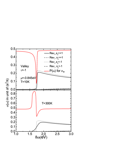
Figure 5: Results for the absorptive part of the conductivity for circularly polarized light, $\sigma_{\pm}(\omega)\equiv\sigma_{xx}\pm i\sigma_{xy}$. Here the valley index $\tau=-1$. The solid is for $Re\sigma_{+}$ the dashed for $Re\sigma_{-}$ both for spin index $s_{z}=+1$. For$s_{z}=-1$ the dotted curve is $\sigma_{+}$ and the dashed dotted for $\sigma_{-}$. The dominant response in this valley is from $\sigma_{+}$ right handed circular polarization, also shown on the same figure is the up to up plus down spin polarization for $\sigma_{+}$ (solid red curve). The top frame is at $T=10K$ and the bottom at $T=300K$.

In Figure 5 we present our results for $Re\sigma_{\pm}(\omega)$ vs. $\omega$ in units of $e^{2}/\hbar$ for valley $\tau=-1$ in the case $\mu=-0.845eV$. The top frame applies to $T=10K$ while temperature is $300K$ in the bottom frame. Results are presented separately for $s_{z}=\pm 1$. We note that $Re\sigma_{+}(\omega)$ is large and comparable in size for either spin up or down while $Re\sigma_{-}(\omega)$ is very small in comparison. This is understood from the optical selection rule which apply to $\sigma_{xx}$ and $\sigma_{xy}$. In the infinite band limit we can show that

$$Re\sigma_{xx}(\omega)\mp Im\sigma_{xy}(\omega)=-\frac{e^{2}}{16\hbar}\theta(\hbar\omega-(\Delta-\lambda))\times$$

$$[1\pm\frac{(\Delta-\lambda)}{\hbar\omega}]^{2}[f(\frac{\lambda}{2}+\frac{\hbar\omega}{2}-\mu)-f(\frac{\lambda}{2}-\frac{\hbar\omega}{2}-\mu)]$$ (16)

which implies a perfect cancelation at the onset energy $\omega=(\Delta-\lambda)$. Here the equation (16) is for $s_{z}=+1$ band with $-\lambda\rightarrow\lambda$ for $s_{z}=-1$ case. Effectively light polarization provides valley selection to a very good approximation. It is exact at the onset energy and remains quite good even at $\omega=4eV$, for which energy the light polarization will reduce the absorption from this valley to about $20\%$ its value for the opposite polarization. The polarization selection rule found here for the dynamical conductivity agree fully with those previous discussed by Yao et.al [13] for inversion symmetry breaking Hamiltonian in two valley systems, where they relate the optical selection rule to the orbital magnetic moment and the Berry curvature of particular valley considered. It is interesting to look at the spin up spin down admixture of the optical response $Re\sigma_{+}(\omega)$ vs. $\omega$. We define

$$P(\omega)=\frac{\sigma_{+}^{spin\text{ }up}(\omega)}{\sigma_{+}^{spin\text{ }up}(\omega)+\sigma_{+}^{spin\text{ }down}(\omega)}$$ (17)

The results are shown as the red curve in Figure 5. We note that for most frequencies $P(\omega)$ is close to $1/2$ but that around the onset energy for $\sigma_{+}$ there is a region where $P(\omega)$ falls below this value and can be close to $0$. This is easily understood as a direct consequence of the displacement in onset between $Re\sigma_{+}(\omega)$ for spin down (dotted curve) and for spin up (solid curve) which implies a deficit of spin up electron in the region between these two onsets. Temperature can have a large effect on the position and shape of $P(\omega)$ in the region of the onset as seen in the lower frame of Figure 5. This can be traced to the fact that the spin up electrons are much more susceptible to temperature smearing for the case considered here as we have already noticed. The solid curve ($\uparrow$) for $\sigma_{+}$ now extend to lower energies than does the short dashed curve ($\downarrow$). Temperature can in fact change the magnitude of $P(\omega)$ in the region of interest from less than $1/2$ to larger than $1/2$ with this entire region shifted toward lower energies. The peak in $P(\omega)$ for $T=300K$ is also broaden as compared with the valley in this same quantity for $T=10K$. The spin admixture in this region can be manipulated with temperature.

V Summary and Conclusions

We presented expressions for the dynamic conductivity of $MoS_{2}$ based on a simplified Hamiltonian which includes spin orbit coupling and band structure parameters fit to first principle calculations. Using the Kubo formula, the final expressions reduce to a sum over momentum $k$ centred about the two valley points $K$ and $-K$ defining the corners of the honeycomb lattice in the Brillouin zone. The bands are spin polarized and a sum over spin and valley appears. The transverse conductivity is split into charge, spin and valley Hall conductivity and, in all cases, depends on an overlap of the Berry curvature multiplied with a common sum of two energy denominators linear in frequency plus appropriate temperature factors and channel dependent indices. The expression for the longitudinal conductivity is not quite as simple but reduces to the common form around $k=0$ (zero momentum). Simplified analytic expressions can be obtained in the infinite band limit. We have presented numerical results for all these quantities as a function of photon energy separating out, in each case, the contribution from the separate spin channels. In the numerical calculations we use a cut off on momentum of $ka=3.0$. The results are not qualitatively different from the infinite band case although there are important quantitative differences. The effect of temperature is considered. It provides a smearing that tends to obscure the separate contributions to the conductivity. It also can change very significantly the spin admixture in the frequency window just above the main absorption threshold where there can be an important imbalance between up and down spin, for a given valley when circular polarized light is employed. The absorptive part of the conductivity for right and left handed polarized light, which is the appropriate quantity for valleytronics is also computed, and it is found that second valley contributes very little to the absorption. For example it is less than $20\%$ at $\omega=4eV$. with main absorption peak at $~{}1.7eV$. The DC limit of the Hall conductivities is obtained analytically. For the parameters appropriate to $MoS_{2}$, the real part of the valley Hall conductivity is positive and large in value as compared with its spin Hall counterpart which is negative for some values of the chemical potential. We hope that our calculations can help further our understanding of the optical properties of $MoS_{2}$.

References

References

- [1] K. S. Novoselov, A. K. Geim, S. V. Morozov, D. Jiang, Y. Zhang, S. V. Dubonos, I. V. Grigorieva and A. A. Firsov, Science 306 , 666 (2004).
- [2] X. Zhang, Y.-W. Tan, H. L. Stormer and P. Kim, Nature 438, 201 (2005).
- [3] K. S. Novoselov, D. Jiang, F. Schedin, T. J. Booth, V. V. Khotkevich, S. V. Morozov, and A. K. Geim, Proc. Natl. Acad. Sci. USA 102, 10451(2004).
- [4] D. Xiao, G. B. Liu, W. Feng, X. Xu and W. Yao, Phys. Rev. Lett. 108, 196802 (2012).
- [5] H. Zeng, J. Dai, W. Yao, D. Xiao and X. Cui, Nature Nano. 7, 490 (2012).
- [6] K. F. Mak, K. He, J. Shan and T. F. Heinz, Nature Nano. 7, 494 (2012).
- [7] T. Cao, G. Wang, W. Han, H. Ye, C. Zhu, J. Shi, Q. Niu, P. Tan, E. Wang, B. Liu and J. Feng, Nature Communications. 3, 887 (2012).
- [8] S. A. Wolf, D. D. Awschalom, R. A. Buhrman, J. M. Daughton, S. von Molnar, M. L. Roukes, A. Y. Chtchelkanova and D. M. Treger, Science 294, 1488, (2001).
- [9] J. Fabian, A. Matos-Abiague, C. Ertler, P. Stano and I. Zutic, Acta Physica Slovaca 57, No.4,5, 565-907, (2007).
- [10] D. Xiao, W. Yao and Q. Niu, Phys. Rev. Lett. 99, 236809 (2007).
- [11] A. Rycerz, J. Tworzydło and C. W. J. Beenakker, Nature Physics, 3, 172 (2007).
- [12] K. Behnia, Nature Nanotechnology, 7, 488 (2012).
- [13] W. Yao, D. Xiao and Q. Niu, Phys. Rev. B 77, 235406 (2008).
- [14] W. Feng, Y. Yao, W. Zhu, J. Zhou, W. Yao and D. Xiao, Phys. Rev. B. 86, 165108 (2012).
- [15] M. Jablan, H. Buljan and M. Soljacic, Phys. Rev. B. 80, 245435 (2009).
- [16] A. Y. Nikitin, F. Guinea, F. J. Garcia-Vidal and L. Martin-Moreno, Phys. Rev. B. 84, 195446 (2011)
- [17] Ashkan Vakil and Nader Engheta, Science 332, 1291 (2011)
- [18] F. Koppens, D. E. Chang and F. J. García de Abajo, Nano letters. 11(8), 3370 (2011)
- [19] J. Chen et.al, Nature 487, 77-81 (2012)
- [20] Z. Fei et.al, Nature 487, 82-85 (2012)
- [21] Z. Y. Zhu, Y. C. Cheng and U. Schwingenschlögl, Phys. Rev. B 84, 153402 (2011).
- [22] T.Li and G. Galli, J. Phys. Chem. C 111, 16192 (2007).
- [23] K. F. Mak, C. Lee, J. Hone, J. Shan and T. F. Heinz, Phys. Rev. Lett. 105, 136805(2010).
- [24] T. Cheiwchanchamnangij and W. R. L. Lambrecht, Phys. Rev. B 85, 205302 (2012).
- [25] A. H. Castro Neto, F. Guinea, N. M. R. Peres, K. S. Novoselov and A. K. Geim, Rev. Mod. Phys.81, 109 (2009).
- [26] V. N. Kotov, B. Uchoa, V. M. Pereira, F. Guinea and A. H. Castro Neto, Rev. Mod. Phys.84, 1067 (2012).
- [27] For silicene, a simpler Hamiltonian applies for which the linear term in the energy of equation (3) is missing. The issues of interest and the parameters used are also quite different. See L. Stille, C. J. Tabert and E. J. Nicol, submitted to Phys. Rev. B.
- [28] V. P. Gusynin, S. G. Sharapov and J. P. Carbotte, Phys. Rev. Lett. 96, 256802 (2006).
- [29] E. J. Nicol and J. P. Carbotte, Phys. Rev. B 77, 155409 (2008).
- [30] T. Stauber and N. M. R. Peres, J. Phys. Conds. Matt. 20, 055002 (2008).
- [31] W. K. Tse and A. H. MacDonald, Phys. Rev. Lett. 105, 057401 (2010).