GPU-accelerated generation of
correctly-rounded elementary functions

Abstract

The IEEE 754-2008 standard recommends the correct rounding of some elementary functions. This requires to solve the Table Maker’s Dilemma which implies a huge amount of CPU computation time. We consider in this paper accelerating such computations, namely Lefèvre algorithm on Graphics Processing Units (GPUs) which are massively parallel architectures with a partial SIMD execution (Single Instruction Multiple Data).

We first propose an analysis of the Lefèvre hard-to-round argument search using the concept of continued fractions. We then propose a new parallel search algorithm much more efficient on GPU thanks to its more regular control flow. We also present an efficient hybrid CPU-GPU deployment of the generation of the polynomial approximations required in Lefèvre algorithm. In the end, we manage to obtain overall speedups up to 53.4x on one GPU over a sequential CPU execution, and up to 7.1x over a multi-core CPU, which enable a much faster solving of the Table Maker’s Dilemma for the double precision format.

1 Introduction

1.1 Problem

The IEEE 754 standard specifies since 1985 the implementation of floating-point operations in order to have portable and predictable numerical software. In its latest revision in 2008 [1], it defines formats (binary32, binary64 and binary128), rounding modes (to the nearest and toward 0, $-\infty$ and $+\infty$) and operations $(+,-,\times,/,\sqrt{\leavevmode\nobreak\ })$ returning correctly rounded values.

Furthermore, it recommends correct rounding of some elementary functions, like log, exp and the trigonometric functions. As these functions are transcendental, one cannot evaluate them exactly but have to approximate them. However, it is hard to decide which intermediate precision is required to guarantee a correctly rounded result – the rounded evaluation of the approximation must be equal to the rounded evaluation of the function with infinite precision. This problem is known as the Table Maker’s Dilemma or TMD [2, chap. 12].

1.2 State of the art

There exist theoretical bounds on the intermediate precision required for correctly rounded functions [2, chap. 12], but these are not sharp enough for efficient floating-point implementations of elementary functions. For example the Nesterenko-Waldschmidt bound for the exponential in double precision gives that $7.290.678$ bits of intermediate precision suffice to provide a correctly rounded result. Hence ad hoc methods are needed to find a sharper bound for each function.

A first method introduced by Ziv [3] was to compute an approximation $y$ of a function value $f(x)$ with a bounded error of $\epsilon$ (containing mathematical and round-off errors). As rounding modes are monotonic, if $y-\epsilon$ and $y+\epsilon$ round to the same floating-point number, $f(x)$ does too : otherwise the correct rounding cannot be determined (see Fig. 1). Hence having a correctly rounded result of $f(x)$ can be done by refining the approximation $(y,\epsilon)$ – decreasing $\epsilon$ – until $y-\epsilon$ and $y+\epsilon$ round to the same floating-point number. For the most common elementary functions, such an $\epsilon$ exists according to the Lindemann–Weierstrass theorem when the function is evaluated at almost all floating-point numbers [4].

Figure 1: Example of undetermined correct rounding for rounding to nearest, where the rounding breakpoints are the midpoints of floating-point numbers.

However, the computation of many approximations can be avoided by precomputing an $\epsilon$ guaranteeing correct-rounding of the evaluation of $f$ at any floating-point number argument. This has to be done by finding the hardest-to-round arguments of the function, that is to say the arguments requiring the highest precision to be correctly rounded when the function is evaluated at. This precision guaranteeing the correct rounding for all arguments is named the hardness-to-round of the function. The hardest-to-round cases can be found by invoking Ziv algorithm at every floating-point number in the domain of definition of the function, but this is prohibitive ($O(2^{p})$ when considering precision-$p$ floating point numbers as arguments).

The first improvement was proposed by Lefèvre, Muller and Tisserand in [5] (Lefèvre algorithm). The main idea of their algorithm is to split the domain of definition into several domains $D_{i}$, to “isolate” hard-to-round cases (HR-cases), and then to use Ziv algorithm to find the hardest-to-round cases among them. This isolation is efficiently performed using local affine approximations of the targeted function over $O(2^{2p/3})$ domains $D_{i}$. Stehlé, Lefèvre and Zimmermann extended this method in 2003 [6] (SLZ algorithm) for higher degree approximations, using the Coppersmith method for finding small roots of univariate modular equation over $O(2^{p/2})$ domains $D_{i}$.

1.3 Motivations and contributions

Even if they are asymptotically and practically faster than exhaustive search, Lefèvre and SLZ algorithms remain very computationally intensive. For example, Lefèvre algorithm requires around five years of CPU time for the exponential function over all double precision arguments, and the SLZ algorithm takes around eight years of CPU time for the function $2^{x}$ over extended double precision arguments in the interval $[1/2,1]$. Moreover, even if the hardest-to-round cases of some functions in double precision are known [2, chap. 12.5], it is still not the case for about half of the univariate functions recommended by the IEEE standard 754-2008. Furthermore, we still have no efficient way to find those of any elementary function in double precision, and quadruple precision is out of reach. We will hence be interested in accelerating the search of hardest-to-round case in double precision (binary64).

As both algorithms split the domain of definition of the targeted function into domains $D_{i}$ and search for HR-cases in them independently, these computations are embarrassingly and massively parallel. The purpose of this work is therefore to accelerate these computations on Graphics Processing Units (GPUs), which theoretically perform one order of magnitude better than CPUs thanks to their massively parallel architectures.

We will focus here on Lefèvre algorithm, which has been used to generate all known hardness-to-round in double precision [2, chap. 12.5]. It is asymptotically less efficient than SLZ as it considers more domains $D_{i}$ ($O(2^{2p/3})$ against $O(2^{p/2})$). However, it performs less operations per domain $D_{i}$ ($O(\log p)$ against $O(\operatorname{poly}(p))$). Therefore, Lefèvre algorithm is as efficient as SLZ in practice for finding the hardness-to-round of elementary functions for double precision format [7] [2, chap. 12] and offers fine-grained parallelism, making it suitable for GPU.

In [8], we discussed implementation techniques to deploy the original Lefèvre algorithm efficiently on GPU which led to an average speedup of 15.4x with respect to the reference CPU implementation on one CPU core. The major bottleneck of this GPU deployment was the control flow divergence which is penalizing considering the partial SIMD execution (Single Instruction Multiple Data) of the GPU. Hardware [9] and software [10, 11] general solutions have been proposed recently to address this problem on GPU. However, these solutions are not efficient in our context as we have a very fine computation grain for each GPU thread. Hence we here focus on algorithmic solutions to tackle directly the origin of this divergence issue.

In this paper, we thus redesign Lefèvre algorithm with the continued fraction formalism, which enables us to get a better understanding of it and to propose a much more regular algorithm for searching HR-cases. More precisely, we strongly reduce two major sources of divergence of Lefèvre algorithm: loop divergence and branch divergence. We also propose an efficient hybrid CPU-GPU deployment of the generation of polynomial approximations $D_{i}$ using fixed multi-precision operations on GPU. These contributions enable on GPU an overall speedup of 53.4x over Lefèvre’s original sequential CPU implementation, and of 7.1x over six CPU cores (with two-way SMT). Finally, as we obtain in the end the same HR-cases as Lefèvre, de Dinechin and Muller experiments [7, 12] we also strengthen the confidence in the generated HR-cases.

1.4 Outline

We will first introduce some notions on GPU architecture and divergence in Sect. 2. Then we will present in Sect. 3 some mathematical background on the Table Maker’s Dilemma and properties of the set $\{a\cdot x\mod{1}\leavevmode\nobreak\ |\leavevmode\nobreak\ x<n\}$ with $a$ fixed. In Sect. 4, we will detail the HR-case search step of Lefèvre algorithm and of the new and more regular algorithm. In the same Sect. 4, we will also present their deployment on GPU. In Sect. 5 we will detail how to efficiently generate on GPU the polynomial approximations $D_{i}$ needed by the two HR-case searches. And finally, we will present performance results in Sect. 6 and conclude in Sect. 7.

2 GPU computing

Graphics Processing Units (GPUs) are many-core devices originally intended for graphics computations. However since mid-2000s they became increasingly used for high performance scientific computing since their massively parallel architectures theoretically perform one order of magnitude better than CPUs, and since general-purpose languages adapted to GPUs like CUDA [13] and OpenCL [14] have emerged. In this section we briefly describe the architecture of the NVIDIA GPU used to test our deployments (the Fermi architecture), GPU programming in CUDA and the divergence problems arising from the partial SIMD execution on GPU. We use here the CUDA nomenclature.

2.1 GPU architecture and CUDA programming

From a hardware point of view, a GPU is composed of several Streaming Multiprocessors denoted SM (14 on Fermi C2070), each being a SIMD unit (Single Instruction Multiple Data) [15]. A SM is composed of multiple execution units or CUDA cores (32 on Fermi) sharing the same pipeline and many registers (32768 on Fermi). GPU memory is organized in two levels: device memory, which can be accessed by any SM on the device; and shared memory, which is local to each SM. The device memory accesses are cached on the Fermi architecture.

From a software point of view, the developer writes in CUDA a scalar code for one function designed to be executed on the device, namely a kernel. At runtime, many threads are created by blocks and bundled into a grid to run the same kernel concurrently on the device. Each block is assigned to a SM. Within each block, threads are executed by groups of 32 called warps. The ratio of the number of resident warps (number of warps a SM can process at the same time) to the maximum number of resident warps per SM is named the occupancy. In order to increase the occupancy the number of blocks and their sizes have to be tuned.

2.2 Divergence

As threads are executed by warps on the GPU SIMD units, applications should have regular patterns for memory accesses and control flow.

The regularity of memory accesses patterns is important to achieve high memory throughput. As the threads within a warp load data from memory concurrently, the developer has to coalesce accesses to device memory and avoid bank conflicts in the shared memory [13, chap. 6]. This can be done by reorganizing data storage.

The regularity of control flow is important to achieve high instruction throughput, and is obtained when all the threads within a warp execute the same instruction concurrently [13, chap. 9]. In fact, when the threads of a same warp diverge (i.e. they follow different execution paths), the different execution paths are serialized. For an if statement, the then and else branches are serially executed. For a loop, any thread exiting the loop has to wait until all the threads of its warp exit the loop. In the following we will distinguish branch divergence due to if statements and loop divergence due to loop statements.

The impact of branch divergence can be statically estimated by counting the number of instructions issued within the scope of the if statement. Let us consider the then branch issues $n_{then}$ instructions and the else branch issues $n_{else}$ instructions. If the warp does not diverge, either $n_{then}$ or $n_{else}$ instructions are issued depending on the evaluation of the condition. If the warp diverges, $n_{then}+n_{else}$ instructions are issued.

Contrary to branch divergence, measuring the impact of loop divergence requires a dedicated indicator and profiling. We introduced in [8] the mean deviation to the maximum of a warp. This indicator is similar to the standard deviation, which is the mean deviation to the mean value. However, as the number of loop iterations issued for a warp is equal to the maximum number of loop iterations issued by any thread within the warp, it is relevant to consider the mean deviation to the maximum value. This gives the mean number of loop iterations a thread remains idle within its warp. More formally, we denote $\ell_{i}$ the number of loop iterations of the thread $i$ and we number the threads within a warp from $1$ to $32$. If $\ell=\{\ell_{i},i\in\llbracket 1,32\rrbracket\}$, the Mean Deviation to the Maximum (MDM) of a warp is defined as

$$\text{MDM}({\ell})=\text{max}(\ell)-\text{mean}(\ell).$$

We can normalize the mean deviation to the maximum by $\displaystyle{\text{max}(\ell)}$ to compute the average percentage of loop iterations for which a thread remains idle within its warp. Hence, the Normalized Mean Deviation to the Maximum (NMDM) is

$$\text{NMDM}(\ell)=1-\frac{\text{mean}(\ell)}{\text{max}(\ell)}.$$

3 Mathematical preliminaries

In this section we give some definitions to introduce more formally the Table Maker’s Dilemma. We also recall some known properties on the distribution of the elements of the set $\{a\cdot x\mod{1}\leavevmode\nobreak\ |\leavevmode\nobreak\ x<n\}$ with a fixed [16], as well as the corresponding continued fraction formalism.

3.1 The Table Maker’s Dilemma

Before defining the Table Maker’s Dilemma, we introduce some notations and definitions. We denote $\{X\}$ or $X\mod{1}$ the fractional part of $X$. We write $X\leavevmode\nobreak\ \operatorname{cmod}\leavevmode\nobreak\ 1$ the centered modulo, which is the real $Y$ such that $X-Y\in\mathbb{Z}$ and $Y\in\leavevmode\nobreak\ ]{-1/2},1/2]$ ($Y$ equals $X-\lfloor X\rfloor$ or $X-\lceil X\rceil$ depending on which has the lowest absolute value). We also write $\mathbb{F}_{p}$ the set of precision-$p$ floating point numbers and $\#_{p}E$ the number of precision-$p$ floating-point numbers in the set $E$ (namely $\#(E\cap\mathbb{F}_{p})$ ).

Definition 1.

The mantissa $m(x)$ and the exponent $e(x)$ of a non-zero real number $x$ are defined by $|x|=m(x)\cdot 2^{e(x)}$ with $1/2\leq m(x)<1$.

Definition 2.

We define $\operatorname{dist}_{p}(x)=|2^{p}\cdot m(x)\leavevmode\nobreak\ \operatorname{cmod}\leavevmode\nobreak\ 1|$ as the scaled distance between a real number $x$ and the closest precision-$p$ floating-point number.

Definition 3.

We now define a $(p,\epsilon)$ hard-to-round case (or HR-case) of a real-valued function $f$ as a precision-$p$ floating-point number $x$ solution of the inequality

$$\operatorname{dist}_{p}(f(x))<\epsilon.$$

The given definition of HR-case only applies for directed rounding. However, this definition can be extended to all IEEE-754 rounding modes as rounding-to-nearest $(p,\epsilon)$ HR-cases are directed rounding $(p+1,2\epsilon)$ HR-cases. To simplify notations, we will then focus on directed rounding HR-cases.

It has to be noticed that if $x$ is a $(p,\epsilon)$ hard-to-round case, it also satisfies $2^{p}\cdot m(f(x))+\epsilon<2\epsilon\mod{1}.$ The latter inequality is used to test if an argument is a $(p,\epsilon)$ HR-case as it avoids the computation of absolute values and cmod.

Hence, a $(p,2^{-p^{\prime}})$ HR-case $x$ is a precision-$p$ floating-point number for which $f(x)$ is at a scaled distance (as defined in Def. 2) less than $2^{-p^{\prime}}$ from the closest precision-$p$ floating-point number. In other words, more than $p+p^{\prime}$ bits of accuracy are necessary to correctly round $f(x)$ at precision-$p$.

Definition 4 (Table Maker’s Dilemma).

If $f$ is a real valued function defined over a domain $D$, we define the Table Maker’s Dilemma as finding a non trivial lower bound on $\{\operatorname{dist}_{p}(f(x)),x\in D\}$.

Figure 2: Distances between the curve defined by $f$ and the rounding breakpoints for rounding-to-nearest.

We call hardest-to-round cases the arguments $x\in D$ minimizing $\operatorname{dist}_{p}(f(x))$. Knowing the hardest-to-round cases gives us a lower bound on the distances between the function $f$ and the rounding breakpoints (see Fig. 2) and therefore a solution to the TMD.

The general method to find the hardest-to-round cases of a function is the following:

1. fix a “convenient” $\epsilon$ using probabilistic assumptions [2, Sect. 12.2],

2. find $(p,\epsilon)$ HR-cases with ad hoc methods such as Lefèvre or SLZ algorithms,

3. find the hardest-to-round among the $(p,\epsilon)$ HR-cases using Ziv method [3].

The most compute intensive step in this method is the second one. Lefèvre or SLZ algorithms both relies on the following three major steps.

1. The split of the domain of definition of the function : we split the domain of definition of the function in $d$ domains $D_{i}=[X_{i},X_{i+1}[\leavevmode\nobreak\ \cap\leavevmode\nobreak\ \mathbb{F}_{p}$ such that, $e(x)=e(y)\leavevmode\nobreak\ \forall x,y\in D_{i}$ and $\#_{p}D_{i}=\#_{p}D_{j}\leavevmode\nobreak\ \forall i,j\in\llbracket 0,d-1\rrbracket$.

2. The generation of polynomial approximations : given a relative error $\epsilon_{approx}$, we approximate the function $f(X)$ with $X\in D_{i}$ by polynomials $P_{i}(x)$ with $x\in\llbracket 0,\#_{p}D_{i}-1\rrbracket$ such that $|P_{i}(x)-f(X)|<\epsilon_{approx}2^{e(f(X))-p}$. We thus proceed to a change of variable enabling to test the floating-point arguments $X\in D_{i}$ by testing the integers $x\in\llbracket 0,\#_{p}D_{i}-1\rrbracket$. Each polynomial $P_{i}$ is first centered on the domain $D_{i}$ by applying the change of variable $\phi_{1}:X\mapsto X-X_{i}$. Then, as the exponent is constant over each domain $D_{i}$, we will consider integer arguments by applying the change of variable $\phi_{2}:X\mapsto X\cdot 2^{p-e(X_{i})}$. All in all, $x=\phi_{2}\circ\phi_{1}(X)=2^{p-e(X_{i})}(X-X_{i})$.

3. The HR-case search: we find the $(p,\epsilon^{\prime})$ HR-cases of $P_{i}$ with $\epsilon^{\prime}=\epsilon+\epsilon_{approx}$ which are the $(p,\epsilon)$ HR-cases for $f$ in $D_{i}$.

In the HR-case search of both algorithms, a Boolean test is used to isolate HR-cases. It successes if there is no $(p,\epsilon^{\prime})$ HR-case for $P_{i}$ in $D_{i}$ and fails otherwise.

In this paper, we focus on Lefèvre algorithm which truncates polynomials $P_{i}$ to degree one for the Boolean test. We denote $Q_{i}(x)=P_{i}(x)\mod{x^{2}}$ the truncation of $P_{i}$ to degree one with $|Q_{i}(x)-P_{i}(x)|<\epsilon_{trunc}2^{e(P_{i}(x))-p}$, and

$$2^{p}\cdot m(Q_{i}(x))+\epsilon^{\prime\prime}=b-a\cdot x,$$

with $\epsilon^{\prime\prime}=\epsilon^{\prime}+\epsilon_{trunc}$. Hence, the Boolean test of Lefèvre algorithm consists of testing if the following inequality holds:

$$\min{\{b-a\cdot x\mod{1}\leavevmode\nobreak\ |\leavevmode\nobreak\ x<\#_{p}D_{i}\}}<2\epsilon^{\prime\prime}.$$ (1)

More precisely, if the inequality (1) does not hold, the Boolean test returns Success as there is no $(p,\epsilon^{\prime\prime})$ HR-cases for $Q_{i}$ in $D_{i}$ which implies there is no $(p,\epsilon^{\prime})$ HR-case for $P_{i}$ in $D_{i}$. Else, it returns Failure. Moreover, we remark that computing the minimum of the set $\{b-a\cdot x\mod{1}\leavevmode\nobreak\ |\leavevmode\nobreak\ x<\#_{p}D_{i}\}$ is similar to finding the multiple of $a$ which is the closest to the left of $b$ modulo $1$ on the unit segment.

3.2 Properties of the set $\{a\cdot x\mod{1}\leavevmode\nobreak\ |\leavevmode\nobreak\ x<n\}$

Here we will detail some properties on the configurations of the points $\{a\cdot x\mod{1}\leavevmode\nobreak\ |\leavevmode\nobreak\ x<n\}$ over the unit segment. These properties are necessary to efficiently locate the closest point to $\{b\}$ in these configurations as we need a Boolean test over a lower bound on $\{b-a\cdot x\mod{1}\leavevmode\nobreak\ |\leavevmode\nobreak\ x<\#_{p}D_{i}\}$.

Theorem 1 (Three distance theorem [17]).

Let $0<a<1$ be an irrational number. If we place on the unit segment $[0,1[$ the points $\{0\}$, $\{a\}$, $\{2a\}$, $\dots$, $\{(n-1)a\}$, these points partition the unit segment into $n$ intervals having at most three lengths with one being the sum of the two others.

Figure 3: Example of configurations generated by $a=14/45$. The unit segment is scaled by a factor $45$ for clarity. Each two-length configuration is labelled by its index $(i,t)$ on the right.

Actually, the lengths and the distribution of these lengths heavily rely on the continued fraction expansion of $a$ [16], which we will denote by

$$a=\cfrac{1}{k_{1}+\cfrac{1}{k_{2}+\ddots}}.$$

We denote by $(\theta_{i})_{i\in\mathbb{N}}$ the sequence of the remainders computed during the continued fraction expansion of $a$ using the Euclidean algorithm, and by $(p_{i}/q_{i})_{i\in\mathbb{N}}$ the sequence of the convergents of $a$, defined by the following recurrence relations :

$$\begin{array}[]{lll}p_{-1}=1&p_{0}=0&p_{i+1}=p_{i-1}+k_{i+1}\cdot p_{i},\\ q_{-1}=0&q_{0}=1&q_{i+1}=q_{i-1}+k_{i+1}\cdot q_{i},\\ \theta_{-1}=1&\theta_{0}=a&\theta_{i+1}=\theta_{i-1}-k_{i+1}\cdot\theta_{i},\end{array}$$

with $k_{i+1}=\lfloor\theta_{i-1}/\theta_{i}\rfloor$. It has to be noticed that $(\theta_{i})_{i\in\mathbb{N}}$ is a decreasing real-valued positive sequence whereas $(p_{i})_{i\in\mathbb{N}}$ and $(q_{i})_{i\in\mathbb{N}}$ are increasing integer-valued positive sequences. We also define $\theta_{i-1,t}=\theta_{i-1}-t\cdot\theta_{i}$ and $q_{i-1,t}=q_{i-1}+t\cdot q_{i}$ with $t\in\llbracket 0,k_{i+1}\llbracket$. The lengths obtained when adding multiples of $a$ over the unit segment are therefore the elements of the sequence $(\theta_{i,t})_{i\in\mathbb{N},t\in\llbracket 0,k_{i+1}\llbracket}$ [16]. An example is provided in Fig. 3 and Table I. All the properties provided in this section are valid when $a$ is irrational. However, they are also valid for $a$ rational as long as $\theta_{i}\not=0$ (that is to say, until the last quotient of the continued fraction expansion is computed).

i	t	$q_{i-1,t}$	$q_{i}$	$\theta_{i-1,t}$	$\theta_{i}$	$k_{+1}i$
0	0	0	1	45	14	3
	1	1		31
	2	2		17
1	0	1	3	14	3	4
	1	4		11
	2	7		8
	3	10		5
2	0	3	13	3	2	1
3	0	13	16	2	1	2
	1	29		1
4	0	16	45	1	0	1

Table I: Values of $\theta_{i}$, $\theta_{i-1,t}$, $q_{i}$, $q_{i-1,t}$ and $k_{i}$ for each two-length configuration of the example of Fig. 3. As in Fig. 3, the lengths $\theta_{i}$ and $\theta_{i-1,t}$ are scaled by a factor 45.

In the following, we will use some properties on the configurations $\{a\cdot x\mod{1}\leavevmode\nobreak\ |\leavevmode\nobreak\ x<n\}$ which contain intervals of only two different lengths. They are of algorithmic interest as there are only $O(\log n)$ such configurations when $n$ tends to infinity. Each label $(i,t)$, with $i\in\mathbb{N}$ and $t\in\llbracket 0,k_{i+1}\llbracket$, denotes one two-length configuration which verifies the following equation

$$q_{i}\cdot\theta_{i-1,t}+q_{i-1,t}\cdot\theta_{i}=1.$$ (2)

This Equation (2) gives details on the number of intervals of each length. After adding $q_{i}+q_{i-1,t}$ multiples of $a\mod{1}$ over the unit segment, there are exactly two different lengths of intervals over the unit segment : $q_{i}$ intervals of length $\theta_{i-1,t}$ and $q_{i-1,t}$ intervals of length $\theta_{i}$.

A special and noticeable subset of the two-length configurations corresponds to the configurations produced using the division-based Euclidean algorithm. These are the $(i,0)$ configurations, satisfying

$$q_{i}\cdot\theta_{i-1}+q_{i-1}\cdot\theta_{i}=1.$$ (3)

Furthermore we have a way to construct the two-length configurations.

Property 1 (Two-length configurations construction [16]).

Given a two-length configuration $(i,t)$ for some $i\in\mathbb{N}$ and $0\leq t<k_{i+1}$, the next two-length configuration is

$$\left\{\begin{array}[]{ll}(i,t+1)&\text{if}\leavevmode\nobreak\ t<k_{i+1}-1,\\ (i+1,0)&\text{if}\leavevmode\nobreak\ t=k_{i+1}-1.\\ \end{array}\right.$$

To simplify notations, given the $(i,t)$ configuration we will write $(i,t+1)$ its next two-length configuration and assimilate the configuration $(i,k_{i+1})$ to $(i+1,0)$. Property 1 implies that for going from a two-length configuration to the next, the intervals of length $\theta_{i-1,t}$ are split. The way intervals are split is described by the following directed reduction property and illustrated in Fig. 3.

Property 2 (Directed reduction [18]).

Given the two-length configuration $(i,t)$, when constructing the next two-length configuration, intervals of length $\theta_{i-1,t}$ are split into two intervals in this order from left to right :

• one of length $\theta_{i}$ and one of length $\theta_{i-1,t+1}$ if $i$ is even,

• one of length $\theta_{i-1,t+1}$ and one of length $\theta_{i}$ if $i$ is odd.

4 HR-case search on GPU

In this section we describe two algorithms for HR-case search: Lefèvre HR-case search originally described in [19] and our new and more regular HR-case search. Both algorithms make use of Boolean tests which rely on the properties described in Sect. 3.2. Hence, we will describe both of them with continued fraction expansions which give a uniform formalism to explain and compare their different behaviours. Then we will describe how they have been deployed on GPU and the benefit on divergence provided by our new algorithm.

4.1 Lefèvre HR-case search

In [19], Lefèvre presented an algorithm to search for $(p,\epsilon^{\prime})$ HR-cases of a polynomial $P_{i}(x)$. This algorithm relies on a Boolean test on $Q_{i}(x)$ (the truncation of $P_{i}(x)$ to degree one) which computes a lower bound of the set $\{b-a\cdot x\mod{1}\leavevmode\nobreak\ |\leavevmode\nobreak\ x<\#_{p}D_{i}\}$ and returns Success if the inequality (1) does not hold, Failure otherwise.

In Sect. 3.2, we described some properties of the configurations $\{a\cdot x\mod{1}\leavevmode\nobreak\ |\leavevmode\nobreak\ x<n\}$. According to these properties, computing the lengths of the intervals of the two-length configurations can be done efficiently in $O(\log{\#_{p}D_{i}})$ arithmetic operations by computing the continued fraction expansion of $a$. However, if we use continued fraction expansion, we will place more points than $\#_{p}D_{i}$ on the unit segment (at most $2\cdot\#_{p}D_{i}$ if we use the subtraction-based Euclidean algorithm). To take advantage of the efficient construction of the two-length configurations, Lefèvre HR-case search computes the minimum of $\{b-a\cdot x\mod{1}\leavevmode\nobreak\ |\leavevmode\nobreak\ x<n\}$ with $n$ the number of multiples of $a$ placed and $n\geq\#_{p}D_{i}$ . This gives a lower bound on $\{b-a\cdot x\mod{1}\leavevmode\nobreak\ |\leavevmode\nobreak\ x<\#_{p}D_{i}\}$. Then the minimum of $\{\operatorname{dist}_{p}(P_{i}(x))<\epsilon^{\prime}\leavevmode\nobreak\ |\leavevmode\nobreak\ x<\#_{p}D_{i}\}$ is exactly computed by exhaustive search in $O(\#_{p}D_{i})$ arithmetic operations only if required. To minimize this exhaustive search we use a filtering strategy in three phases.

• Phase 1: we compute a lower bound on $\{b-a\cdot x\mod{1}\leavevmode\nobreak\ |\leavevmode\nobreak\ x<\#_{p}D_{i}\}$ and test if this lower bound matches a $(p,\epsilon^{\prime\prime})$ HR-case of $Q_{i}$. If not there is no $(p,\epsilon^{\prime})$ HR-case for $P_{i}$ in $D_{i}$. Else, go to next phase.

• Phase 2: we split $D_{i}$ in sub-domains $D_{i,j}$, we refine the approximation $Q_{i}(x)$ by $Q_{i,j}(x)$ and we compute a lower bound on $\{b_{j}-a_{j}\cdot x\mod{1}\leavevmode\nobreak\ |\leavevmode\nobreak\ x<\#_{p}D_{i,j}\}$ for each $D_{i,j}$. For each $D_{i,j}$ where the lower bound on $\{b_{j}-a_{j}\cdot x\mod{1}\leavevmode\nobreak\ |\leavevmode\nobreak\ x<\#_{p}D_{i,j}\}$ matches a $(p,\epsilon^{\prime\prime}_{j})$ HR-case of $Q_{i,j}$, go to next phase.

• Phase 3: we search exhaustively for $(p,\epsilon^{\prime})$ of $P_{i}$ in $D_{i,j}$ using the table difference method (see Sect. 5).

The corner stone of Lefèvre algorithm strategy is therefore the computation of the minimum of $\{b-a\cdot x\mod{1}\leavevmode\nobreak\ |\leavevmode\nobreak\ x<n\}$. In other words, it computes the distance between $\{b\}$ and the closest point to the left of $\{b\}$ in the configuration $\{a\cdot x\mod{1}\leavevmode\nobreak\ |\leavevmode\nobreak\ x<n\}$. We write $N$ the number of floating-point numbers in the considered sub-domain ($n\geq N$ as we compute a lower bound). Depending on how we generate the two-length configurations (using the subtraction-based or the division-based Euclidean algorithm) we can derive from Property 2 two ways to compute this distance. The first one is Lefèvre HR-case search, the second one is the new HR-case search proposed in Sect. 4.2.

input : $b-a\cdot x$, $\epsilon^{\prime\prime}$, $N$

1 initialisation:

$p\leftarrow\{a\}$;	$q\leftarrow 1-\{a\}$;	$d\leftarrow\{b\}$;
$u\leftarrow 1$;	$v\leftarrow 1$;

2if $d<\epsilon^{\prime\prime}$ then return Failure;

3 while True do

4       if $d<p$ then

5             $k=\lfloor q/p\rfloor$;

6             $q\leftarrow q-k*p$; $u\leftarrow u+k*v$;

7             if $u+v\geq N$ then return Success;

8             $p\leftarrow p-q$; $v\leftarrow v+u$;

9            

10      else

11             $d\leftarrow d-p$;

12             if $d<\epsilon^{\prime\prime}$ then return Failure;

13             $k=\lfloor p/q\rfloor$;

14             $p\leftarrow p-k*q$; $v\leftarrow v+k*u$;

15             if $u+v\geq N$ then return Success;

16             $q\leftarrow q-p$; $u\leftarrow u+v$;

17            

18      

Algorithm 1 Lefèvre lower bound computation and test algorithm.

In the lower bound computation of Lefèvre HR-case search, the way the two-length configurations are computed depends on the length of the interval containing $\{b\}$. When adding points in the interval containing $\{b\}$ and in the direction of $\{b\}$ Lefèvre uses a subtraction-based Euclidean algorithm (he moves from the $(i,t)$ configuration to $(i,t+1)$). Otherwise he uses a division-based Euclidean algorithm (he moves from the $(i,t)$ configuration to $(i+1,0)$). Algorithm 1 describes the lower bound computation of Lefèvre HR-case search and the corresponding test with respect to $\epsilon^{\prime\prime}$ which is the sum of all errors involved.

In this algorithm, the variables $u$ and $v$ count the number of intervals as in Equation (2) in order to exit when $n=u+v\geq N$ : $u$ and $v$ store respectively $q_{i}$ and $q_{i-1,t}$ for $i$ even and $q_{i-1,t}$ and $q_{i}$ for $i$ odd. The variables $p$ and $q$ store respectively the lengths $\theta_{i}$ and $\theta_{i-1,t}$ for $i$ even, and the lengths $\theta_{i-1,t}$ and $\theta_{i}$ for $i$ odd. The variable $d$ contains the distance between $\{b\}$ and the closest multiple $\{a\cdot x\}$ to its left.

(a) $i$ is even

(b) $i$ is odd

Figure 4: Behaviour of Lefèvre (left) and the new (right) HR-case searches when $b$ is in an interval of length $\theta_{i}$ (solid lines) and when $b$ is in an interval of length $\theta_{i-1,t}$ (dashed lines). Each point is labelled by the index $(i,t)$ of the two-length configuration it is added in.

Hereafter we detail the relations between the two-length configurations and the execution paths of Algorithm 1. This algorithm starts with the configuration $(0,1)$ and then considers the $(i,t)$ configurations. It has to be noticed that the condition at line 4 is false only if we added one point directly at the left of $\{b\}$ during the previous loop iteration and true otherwise. Hence, it has to be interpreted as “does $d$ need to be updated?”. This interpretation is allowed by the fact that the value of $d$ at line 4 corresponds to the previous configuration (the configuration $(0,0)$ at start) and that at least one point was already added (line 8 or 15). This condition enables thus to handle the next four cases (illustrated in Fig. 4).

• If $i$ is even:

  • if $\{b\}$ is in an interval of length $\theta_{i}$, then $d<\theta_{i}$ (this happens if the point previously added is just at the right of $\{b\}$). Hence no point is added in the interval containing $\{b\}$ so we go directly to the configuration $(i+1,0)$ (lines 5-6) and $(i+1,1)$ (line 8);

  • if $\{b\}$ is in an interval of length $\theta_{i-1,t}$, then $d>\theta_{i}$ (this case happens if the point previously added is just at the left of $\{b\}$). Hence $d$ is updated by subtracting $\theta_{i}$ (line 10), $k=0$ since $\theta_{i-1,t}>\theta_{i}$ (lines 12-13), and we go to configuration $(i,t+1)$ (line 15) as other points can be added to the left of $\{b\}$ in the next two-length configuration under Property 2.

• If $i$ is odd:

  • if $\{b\}$ is in an interval of length $\theta_{i}$, then $d>\theta_{i-1,t}$ (this case happens if the point previously added is just at the left of $\{b\}$). Hence $d$ is updated (line 10) and we go to the configuration $(i+1,0)$ (lines 12-13) and $(i+1,1)$ (line 15);

  • if $\{b\}$ is in an interval of length $\theta_{i-1,t}$, then $d<\theta_{i-1,t}$ (this case happens if the point previously added is just at the right of $\{b\}$). Hence $k=0$ since $\theta_{i-1,t}>\theta_{i}$ (lines 5-6) and we go to the configuration $(i,t+1)$ (line 8) as a point can be added to the left of $\{b\}$ in the next two-length configuration according to Property 2.

It has to be noticed that Lefèvre algorithm always reduces $d$ by using subtractions at line 10 as points are added one by one at the left of $\{b\}$. In practice Lefèvre adds specific instructions to compute partly these reductions with divisions in order to avoid large quotients to be entirely computed with subtractions. We have omitted these instructions here for clarity but they are present in our implementations of Lefèvre algorithm.

Furthermore the algorithm computes divisions (lines 5 and 12). In practice, we can make use of different division implementations. We can apply a subtractive division, a division instruction, or combine both in an hybrid approach as presented and analysed in [19, 8].

4.2 New regular HR-case search

We here propose a new algorithm for the HR-case search where we use the same filtering and division strategy as in Lefèvre algorithm, but we introduce a more regular algorithm – in the sense that it strongly reduces divergence on GPU – in order to compute a lower bound on $\{b-a\cdot x\mod{1}\leavevmode\nobreak\ |\leavevmode\nobreak\ x<\#_{p}D_{i}\}$. Hereafter, we will refer to this new algorithm as the regular HR-case search.

input : $b-a\cdot x$, $\epsilon^{\prime\prime}$, $N$

1 initialisation:

$p\leftarrow\{a\}$;	$q\leftarrow 1$;	$d\leftarrow\{b\}$;
$u\leftarrow 1$;	$v\leftarrow 0$;

2if $d<\epsilon^{\prime\prime}$ then return Failure;

3 while True do

4       if $p<q$ then

5             $k=\lfloor q/p\rfloor$;

6             $q=q-k*p$; $u=u+k*v$;

7             $d=d\mod p$;

8            

9      else

10             $k=\lfloor p/q\rfloor$;

11             $p=p-k*q$; $v=v+k*u$;

12             if $d\geq p$ then

13                   $d=(d-p)\mod q$;

14                  

15            

16       if $u+v\geq N$ then return $d>\epsilon^{\prime\prime}$;

17      

Algorithm 2 New regular lower bound computation and test algorithm.

In this regular HR-case search described in Algorithm 2, we only consider configurations satisfying Equation (3) in order to use only the division-based Euclidean algorithm. The variables $p$ and $q$ store respectively the lengths $\theta_{i}$ and $\theta_{i-1}$ for $i$ even, and the lengths $\theta_{i-1}$ and $\theta_{i}$ for $i$ odd. The variables $u$ and $v$ store respectively $q_{i}$ and $q_{i-1}$ for $i$ even, and $q_{i-1}$ and $q_{i}$ for $i$ odd.

Thus, instead of testing if $\{b\}$ went from a split interval to an unsplit one like in Lefèvre HR-case search, we test here which length is reduced as in the classical Euclidean algorithm, and then we reduce it and update $d$ accordingly (as illustrated in Fig. 4). In practice, the quotients are computed like in Lefèvre HR-case search with a subtractive division, a division instruction or the hybrid approach. Now we detail the execution of the algorithm. Let $(i,0)$ be a two-length configuration.

• If $i$ is even, then the test $p<q$ is true since $\theta_{i}<\theta_{i-1}$, we go to the configuration $(i+1,0)$ (lines 5-6) and :

  • if $\{b\}$ was in an interval of length $\theta_{i}$, no point was added in the interval containing $\{b\}$ and $d$ is not updated as $d<\theta_{i}$ and $d=d\mod{\theta_{i}}$ (line 7);

  • if $\{b\}$ was in an interval of length $\theta_{i-1}$, points were potentially added to the left of $\{b\}$. Hence the distance $d$ is updated by reduction modulo $\theta_{i}$ (line 7) since intervals are split from the left under Property 2.

• If $i$ is odd, then the test $p<q$ (line 4) is false, we go to the configuration $(i+1,0)$ (lines 9-10) and :

  • if $\{b\}$ was in an interval of length $\theta_{i}$, no point was added in the interval containing $\{b\}$. However, we might subtract $\theta_{i+1}$ to $d$ if $d\geq\theta_{i+1}$ (line 12), which is similar to considering the configuration $(i+1,1)$. Note that this would have been done in the next loop iteration at line 7 (see Fig. 5);

  • if $\{b\}$ was in an interval of length $\theta_{i-1}$, points were potentially added to the left of $\{b\}$. According to Property 2, intervals are split from the right. Then the distance $d$ is updated if $d>\theta_{i+1}$ by reducing $d-\theta_{i+1}\mod\theta_{i}$ (lines 11-12).

Figure 5: Example where Algorithm 2 considers a configuration $(i+1,1)$ for $i=1$.

4.3 Deployment on GPU

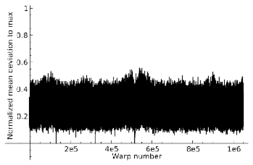
(a) Lefèvre HR-case search with specific instructions

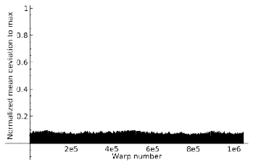
(b) Regular HR-case search

Figure 6: Normalized mean deviation to the maximum of the number of main loop iterations per warp among the $2^{20}$ warps required for the exp function in the domain $[1;1+2^{-13}]$.

The exhaustive search algorithm perfectly takes advantage of the GPU massive parallelism and of its (partial) SIMD execution. Hence, we will focus on the deployment of the lower bound computation. In this section we present the GPU deployment of Lefèvre HR-case search as detailed in [8], and the GPU deployment of the new regular HR-case search. We particularly study the divergence in both HR-case searches at three levels: the filtering strategy, the main loop and the main conditional statement. For these deployments, we first changed the data layout to a “structure of arrays” in order to have coalesced memory accesses [13, Sect. 6.2.1]. We also avoided as much as possible consecutive dependent instructions in order to increase the instruction-level parallelism within each thread.

Throughout this section, we will consider the example domain $[1,1+2^{-13}[$ in the binade $[1,2[$ for the exponential function in double precision, as this binade is considered in [19] as the general case.

4.3.1 Filtering strategy divergence

As a consequence of the filtering strategy, we will have few threads executing phase 2, and fewer executing phase 3. Table II shows the number of sub-domains involved in each phase for a domain $D_{i}$ containing $2^{40}$ floating-point numbers. As we can see, very few sub-domains are concerned by the exhaustive search step. Hence, executing one kernel computing the three phases leads to an important divergence as we have fewer and fewer active threads within each warp from one phase to the next [8].

To tackle this problem, we propose to use three kernels, one for each phase. This allows us to re-build the grid of threads between each phase, and to run the exact number of threads required by each phase. However, this implies two additional costs.

First, we have to write failing sub-domains of phases 1 and 2 in consecutive memory locations as we prepare coalesced reads for the next phase. In [8], this was done with atomic operations on the GPU global memory since we had few failing sub-domains. For some specific binades, the number of failing sub-domains can be much more important and the numerous atomic operations can then lower the performance. Hence, we use atomic operations on the GPU global memory or compact operations based on parallel prefix sums provided by CUDPP [20], depending on the expected number of failing sub-domains.

Second, between two phases, we have to transfer back to CPU the number of failing sub-domains to compute on CPU the optimal grid size for the next phase.

	Number of arguments
	Lefèvre	Regular
Phase 1	$2^{40}\approx 1.1\cdot 10^{12}$	$2^{40}\approx 1.1\cdot 10^{12}$
Phase 2	$\approx 3.6\cdot 10^{9}$	$\approx 1.8\cdot 10^{10}$
Phase 3	$\approx 8.9\cdot 10^{6}$	$\approx 5.9\cdot 10^{7}$
HR-cases	$243$	$243$

Table II: Details of argument filtering during HR-case search in $[1,1+2^{-13}]$.

It can be noticed in Table II that Lefèvre HR-case lower bound computation filters a little more than the new algorithm. Lefèvre HR-case lower bound computation uses indeed subtraction-based Euclidean algorithm when splitting the interval containing $\{b\}$. This results in a number of considered arguments less than $2N$. On the contrary, we always use the division-based Euclidean algorithm in the regular HR-case search. If we consider $i$ such that $q_{i}+q_{i-1}<N<q_{i+1}+q_{i}$, then $q_{i+1}+q_{i}=q_{i-1}+k_{i+1}q_{i}+q_{i}<(k_{i+1}+1)N$ – by considering $q_{i}<N$. However, the geometric mean of the quotients $k_{i}$ of the continued fraction of almost all real numbers equals Khinchin’s constant ($\approx 2.69$) [21]. Hence, using the regular HR-case search we consider on average less than $3.69\cdot N$ arguments.

4.3.2 Loop divergence

HR-case search	min	max	mean	mean
	iteration	iteration	iteration	NMDM
	number	number	number
Lefèvre	$5$	$328$	$24$	$25.6\%$
with specific	$5$	$31$	$16$	$25.7\%$
instructions
Regular	$8$	$19$	$12$	$0.1\%$

Table III: Comparison of the main loop behavior among the $2^{20}$ warps required for the different HR-case searches on exp function in the domain $[1,1+2^{-13}]$.

The second source of divergence is the main unconditional loop (see line 3 in Algorithms 1 and 2). Fig. 6 shows the NMDM of the number of loop iterations by warp for the different HR-case searches when testing a domain $D_{i}$ containing $2^{40}$ double precision floating-point arguments. Table III summarizes statistical informations on the NMDM and the number of iterations for both Lefèvre and the regular HR-case searches.

For Lefèvre HR-case search, this main unconditional loop is an important source of divergence with a mean NMDM of $25.6\%$, that is to say, a thread remains idle on average $25.6\%$ of the number of loop iterations executed by its warp. To our knowledge there is no a priori information on the number of loop iterations that would enable us to statically reorder the sub-domains in order to decrease this divergence. We also tried to use software solutions to reduce the impact of the loop divergence [8] to no avail because the computation is very fine-grained.

This divergence in Lefèvre HR-case search is mainly due to the fact that the quotients are entirely or partially computed at each iteration depending on the position of $b$ even with the specific instructions (see Sect. 4.1). Thanks to these specific instructions the pathological cases are avoided (see Table III) but the mean NMDM is still around $25.6\%$.

In the new regular HR-case search, the key point is that a quotient of the continued fraction expansion of $a$ is entirely computed at each loop iteration, which is not the case in Lefèvre HR-case search. Hence, the number of loop iterations only depends on the number of quotients of the continued fraction expansion of $a$ computed to reach $\#_{p}D_{i}$ points on the segment. As the number of quotients to compute is very close from one sub-domain to the next, we reduce the mean NMDM by warp to $0.1\%$.

4.3.3 Branch divergence

The third source of divergence is on the main conditional statement (see line 4 in Algorithms 1 and 2). We aim at reducing the number of instructions controlled by the branch condition, and if reduced enough, benefit from the GPU branch predication [13, Sect. 9.2]. This branch predication enables indeed, for short sections of divergent code, to fill at best the pipelines by scheduling both then and else branches for all threads: thank to a per-thread predicate, only the relevant results are actually computed and finally written.

input : $b-a\cdot x$, $\epsilon^{\prime\prime}$, $N$

1 initialisation:

$p\leftarrow\{a\}$;	$q\leftarrow 1-\{a\}$;	$d\leftarrow\{b\}$;
$u\leftarrow 1$;	$v\leftarrow 1$;	$are\_swapped\leftarrow False$;

2if $d<\epsilon^{\prime\prime}$ then return Failure;

3 if $(d\geq p)$ then

4       SWAP$(p,q)$; SWAP$(u,v)$;

5       $are\_swapped\leftarrow True$;

6      

7

8while True do

9       if $are\_swapped$ then

10             $d\leftarrow d-p$;

11             if $d<\epsilon^{\prime\prime}$ then return Failure;

12            

13      

14      $k=\lfloor q/p\rfloor$;

15       $q\leftarrow q-k*p$; $u\leftarrow u+k*v$;

16       if $u+v\geq N$ then return Success;

17       $p\leftarrow p-q$; $v\leftarrow v+u$;

18      

19      if $are\_swapped$ xor $(d\geq p)$ then

20             SWAP$(p,q)$; SWAP$(u,v)$;

21             $are\_swapped\leftarrow not(are\_swapped)$;

22            

23      

Algorithm 3 Lefèvre’s lower bound computation and test algorithm with swap.

As observed in [8], both branches of Lefèvre HR-case search contain the same instructions, except that the variables $p$ (respectively $u$) and $q$ (resp. $v$) are interchanged, and that $p$ is subtracted to $d$ in the else branch. We therefore swap the two values $p$ and $q$ (resp. $u$ and $v$) to remove the common instructions from the conditional scope as described in Algorithm 3. The swap implies a small extra cost but we thus reduce the number of divergent instructions.

input : $b-ax$, $\epsilon^{\prime\prime}$, $N$

1 initialisation:

$p\leftarrow\{a\}$;	$q\leftarrow 1$;	$d\leftarrow\{b\}$;
$u\leftarrow 1$;	$v\leftarrow 0$;

2while True do

3       $k=\lfloor q/p\rfloor$;

4       $q=q-k*p$; $u=u+k*v$;

5       $d=d\mod p$;

6       if $u+v\geq N$ then return $d>\epsilon^{\prime\prime}$;

7      

8      $k=\lfloor p/q\rfloor$;

9       $p=p-k*q$; $v=v+k*u$;

10       if $d\geq p$ then

11             $d=d-p\mod q$;

12            

13       if $u+v\geq N$ then return $d>\epsilon^{\prime\prime}$;

14      

Algorithm 4 New regular lower bound computation and test algorithm unrolled.

As far as the new regular HR-case search is concerned, there is in Algorithm 2 as much branch divergence within the unconditional loop as in Algorithm 1. However the main conditional statements of the two algorithms are rather different. In Lefèvre HR-case search, this test depends on the position of the point $b$ at each iteration. In the regular HR-case search, it depends on the length to reduce. Unlike the test on the position of $b$, the test on the length to reduce is deterministic as the regular HR-case search computes a quotient of the continued fraction expansion of $a$ at each loop iteration. Hence the evaluation of the condition switches at each loop iteration and it first evaluates to True as $p$ is initialized to $\{a\}$ and $q$ to $1$. Therefore, by unrolling two loop iterations (Algorithm 4), we can avoid this test and strongly reduce the branch divergence.

5 Polynomial approximation generation on GPU

In this section, we detail how we have deployed on GPU the generation of the polynomial approximations $P_{i}$ required for the HR-case search algorithms described in Sect. 4. We recall that the change of variable $x=2^{p-e(X_{i})}(X-X_{i})$ enables to test the floating-point arguments $X\in D_{i}$ of $f(X)$ by testing the integer arguments $x\in\llbracket 0,\#_{p}D_{i}-1\rrbracket$ of $P_{i}(x)$.

Computing as many approximations as $D_{i}$ domains can be prohibitive using Taylor approximations. The principle here is therefore to consider the union of $\tau$ domains $D_{t},\dots,D_{t+\tau-1}$ – denoted $\mathcal{D}_{t}$ – and to approximate the function $f$ by a polynomial $R_{t}$ of degree $\delta$ – with a Taylor approximation for example – such that $|R_{t}(x)-f(X)|<\epsilon_{approx}^{\prime}2^{e(f(X))-p}$ for all $X\in\mathcal{D}_{t}$ with $x=2^{p-e(X_{t})}(X-X_{t})$.

If $\tau$ is chosen such that $e(x)=e(y)$ for all $x,y\in\mathcal{D}_{t}$, then $P_{t+i}(x)$ is defined as $R_{t}(x+iN)$ for $0\leq i<\tau$ with $N=\#_{p}D_{t}$ (as $\#_{p}D_{i}=\#_{p}D_{j}\leavevmode\nobreak\ ,\leavevmode\nobreak\ \forall i,j\in\mbox{$\llbracket t,t+\tau-1\rrbracket$}$). The shifts of the form $R_{t}(x+iN)$ are called Taylor shifts [22]. If we denote $\epsilon_{shift}$ the error propagated by the shift such that $|P_{t+i}(x)-R_{t}(x+iN)|<\epsilon_{shift}$, then we set $\epsilon_{approx}$ to $\epsilon_{approx}=\epsilon_{approx}^{\prime}+\epsilon_{shift}$ (see Sect. 3.1).

In the following, we want to compute these polynomials $P_{t+i}$ . We first present a method named the hierarchical method originally designed by Lefèvre [23] to change one Taylor shift by $N$ into several Taylor shifts by $1$. Then, we present two existing Taylor shift algorithms:

• the tabulated difference shift which, starting with $P_{t}(x)=R_{t}(x)$, sequentially iterates a shift of the polynomial $P_{t+i}$ to obtain $P_{t+i+1}$ with only multi-precision additions [7];

• and the straightforward shift which computes the $P_{t+i}$’s from $R_{t}$ in parallel but requires multi-precision multiplications and additions [22].

Finally we propose an hybrid CPU-GPU Taylor shift algorithm which efficiently combines these two shifts with the hierarchical method, and which requires only fixed size multi-precision addition on GPU. More details on these algorithms and their error propagation can be found in [7].

5.1 Hierarchical method

We first describe the hierarchical method originally described in [23] which transforms one shift by $N$ of a polynomial $R_{t}(x)$ of degree $\delta$ into $\delta+1$ shifts by $1$. This is of interest as shifting by $1$ can be done with only additions (see Sect. 5.2). This method requires the input polynomial to be interpolated in the binomial basis $\binom{x}{j}=\frac{\prod_{l=0}^{j-1}{(x-l)}}{j!}$. Therefore, we define the forward difference operator and its application to interpolate a polynomial in the binomial basis.

Definition 5.

The forward difference operator, denoted $\Delta_{h}$ is defined as $\Delta_{h}[P](x)=P(x+h)-P(x)$. We write $\Delta_{h}^{j}$ the composition $j$ times of $\Delta_{h}$ and $\Delta=\Delta_{1}$.

Figure 7: Newton interpolation of polynomial $x^{3}$. The coefficients of the interpolated polynomial are highlighted.

Figure 8: Tabulated difference shift for evaluating the polynomial $r_{t,j}(i)=i^{3}$. The shifted polynomials are highlighted.

Using this forward difference operator, one can efficiently interpolate the polynomial $R_{t}$ of degree $\delta$ in the binomial basis [7], given the values $\{R_{t}(x),x\in\llbracket 0,\delta\rrbracket\}$ as $R_{t}(x)=\sum_{j=0}^{\delta}\Delta^{j}[R_{t}](0)\cdot\binom{x}{j}.$ An example is shown in Fig. 7. This interpolation is computed using the definition of $\Delta$ and with initial values $\Delta^{0}[R_{t}](x)=R_{t}(x)$. This algorithm is similar to the Newton interpolation with the forward difference operator used instead of the forward divided difference operator.

Now, we describe the hierarchical method[23]. Given a polynomial $R_{t}(x)$, we want to build a scheme to shift this polynomial in consecutive arguments following an arithmetic progression with common difference $N$. Let us consider the univariate polynomial $R_{t}$ as a bivariate polynomial $R_{t}(x+iN)$ in the variables $x$ and $i$. By interpolation in the binomial basis with respect to the variable $x$, we obtain a polynomial in the variable $x$, with polynomial coefficients $r_{t,j}(i)=\Delta^{j}[R_{t}](iN)$ in the variable $i$, defined as follow

$$R_{t}(x+iN)=\sum_{j=0}^{\delta}{r_{t,j}(i)\binom{x}{j}}.$$

Using the hierarchical method, we thus obtain the polynomials $r_{t,j}(i)$. From these, one can compute the shifts $P_{t+i}(x)$ of the polynomial $R_{t}(x)$ by $iN$ by computing the evaluations $r_{t,j}(i)$ with $0\leq j\leq\delta$. If we consider the polynomials $r_{t,j}$ in the binomial basis, these evaluations $r_{t,j}(i)$ can be obtained with the consecutive Taylor shifts of $r_{t,j}$ by one – by taking the coefficients of degree $0$ of these shifts, which are the $\Delta^{0}[r_{t,j}](i)$.

5.2 Taylor shift algorithms

Taylor shifts by one can be performed efficiently with the tabulated difference shift [7, 5]. According to the forward difference operator definition, $\Delta^{l}[r_{t,j}](i)=\Delta^{l-1}[r_{t,j}](i+1)-\Delta^{l-1}[r_{t,j}](i),$ that is to say $\Delta^{l-1}[r_{t,j}](i+1)=\Delta^{l-1}[r_{t,j}](i)+\Delta^{l}[r_{t,j}](i).$ Furthermore, if $deg(r_{t,j})=\gamma$ then $\Delta^{\gamma}[r_{t,j}](i)$ is constant for any integer $i\geq 0$, as it is the $\gamma^{th}$ discrete derivative of $r_{t,j}$ times $\gamma!$ . An illustration of this algorithm can be found in Fig. 8. Hence, the only needed operations to obtain the consecutive evaluations of the polynomials $r_{t,j}$ are multi-precision additions of the coefficients.

Obtaining the consecutive evaluations of $r_{t,j}$ can also be performed with the straightforward shift. This algorithm multiplies the vector of the $r_{t,j}$ polynomial coefficients by a matrix constructed using Newton’s binomial theorem. If we consider the polynomials $r_{t,j}$ expressed in the binomial basis, this multiplication exactly corresponds to applying $i$ times the tabulated difference algorithm on the polynomial $r_{t,j}$. This matrix is upper triangular and Toeplitz, which can be used to speed up the matrix-vector multiplication for high degree, and is constructed as

$$\small\begin{pmatrix}\binom{i}{0}&\binom{i}{1}&\cdots&\binom{i}{\gamma}\\ 0&\binom{i}{0}&\cdots&\binom{i}{\gamma-1}\\ \vdots&\ddots&\ddots&\vdots\\ 0&\cdots&0&\binom{i}{0}\end{pmatrix}.$$

Therefore, to construct this matrix, only the first $\binom{i}{l}$ with $0\leq l<\gamma+1$ are needed to compute its coefficients.

5.3 Hybrid CPU-GPU deployment

Now, we propose a hybrid CPU-GPU deployment of the polynomial approximation generation step. The polynomials $R_{t}$ are Taylor polynomials of degree $\delta=2$ approximating the targeted function over $\tau=2^{25}$ domains $D_{i}$ like in [5]. We interpolate them in the binomial basis using the hierarchical method with $N=2^{15}$ as we want to use the Boolean tests described in Sect. 4 on intervals containing $2^{15}$ arguments (this choice of parameters is motivated by the error analysis of the Boolean test [23]). More formally, we have

$$P_{t+i}(x)=R_{t}(i2^{15}+x)=\sum_{j=0}^{2}{r_{t,j}(i)\binom{x}{j}}.$$

As this interpolation in the binomial basis is done once, it is precomputed on CPU.

Hence, to obtain all the polynomials $P_{t+i}$ for $0\leq i<\tau$, we have to deploy on GPU the computation of the consecutive evaluations of $r_{t,j}(i)$ for $0\leq i<\tau$ and $0\leq j\leq 2$.

On one hand, the tabulated difference shift is efficient as it requires only multi-precision additions. This method is thus used in the reference CPU implementation [5]. However this is an intrinsically sequential algorithm, which prohibits its direct deployment on GPU. On the other hand, the straightforward shift is embarrassingly parallel, but requires multi-precision multiplications and divisions to compute the binomials and multi-precision multiplications and additions to compute the matrix-vector products.

In order to benefit from the efficiency of the tabulated difference shift on GPU, we therefore use an hybrid strategy that relies on both the CPU and the GPU: we compute the shifts $r_{t,j,u}(i)=r_{t,j}(u\nu+i)$ to form $\mu$ packets of size $\nu$ such that $\mu\nu=\tau$. We vary $u$ from $0$ to $\mu-1$ and construct the polynomials $r_{t,j,u}$ sequentially on CPU with the straightforward shift. All the multi-precision operations on CPU are computed efficiently using the GMP library [24].

Then the $\mu$ polynomials $r_{t,j,u}$ are transferred to GPU. We run a CUDA kernel of $\mu$ threads wherein each thread of ID $u$ processes the polynomial $r_{t,j,u}$ and computes the evaluations $r_{t,j,u}(i)$ with $0\leq i<\nu$ using the tabulated difference shift.

Furthermore, as there are $\delta+1$ independent $r_{t,j}$ polynomials ($\delta=2$ in practice), we can run one kernel per $r_{t,j}$ polynomial and overlap the GPU tabulated difference shift for the polynomial $r_{t,j}$ with the CPU straightforward shift of the polynomial $r_{t,j+1}$. The only algorithm deployed on GPU is therefore the tabulated difference shift which is sequential within each GPU thread, but performed concurrently by multiple threads on multiple polynomials $r_{t,j,u}$.

As the coefficients of the considered polynomials are large, we need multi-precision addition on GPU. Here only fixed size multi-precision additions are required as bounds on the required precision, depending on the targeted function and exponent of the targeted domain, can be computed before compile time [23, 7]. Multi-precision libraries on GPU [25, 26] have been very recently developed. However, we preferred to have our own implementation of this operation for two main reasons: to use PTX (NVIDIA assembly language) [27] and the addc instruction in order to have an efficient carry propagation; and to benefit from the fixed size of the multi-precision words at compile time in order to unroll inner loops. As the addc instruction operates only on 32-bit words, multi-precision words are arrays of 32-bit chunks. The multi-precision addition function is implemented as a C++ template with the size of the multi-precision words given as a parameter, which enables an automatic generation of addition functions for each size of fixed multi-precision word required by each binade. As a consequence, the inner loop on the number of chunks can easily be unrolled as the number of loop iterations is known at compile time. Furthermore, in order to have coalesced memory accesses, the word chunks are interleaved in global memory and loaded chunk by chunk in registers.

Finally, it can be noticed that this algorithm is completely regular: there is therefore no divergence issue among the GPU threads here.

6 Performance results

In this section we present the performance analysis of our different deployments. All results are obtained on a server composed of one Intel Xeon X5650 hex-core processor running at 2.67 GHz, one NVIDIA Fermi C2070 GPU and 48 GB of DDR3 memory.

We compare three implementations. The first one is the sequential implementation (named Seq.) which is Lefèvre reference code provided by V. Lefèvre. The second one is the parallel implementation on CPU (referred to as MPI) which is the sequential implementation with an MPI layer (OpenMPI version 1.4.3) to distribute equally the $2^{13}$ intervals composing a binade among the available CPU cores. We use a cyclic decomposition which offers a better load balancing than a block decomposition and run 12 MPI processes to take advantage of the two-way SMT (Simultaneous Multithreading or Hyper-Threading for Intel) of each core. The third implementation (named CPU-GPU) relies on the GPU and CPU-GPU deployments presented in this paper. The implementations have been compiled with gcc-4.4.5 for CPU code and nvcc (CUDA 4.1) for GPU code.

All the following timings are obtained for searching $(53,2^{-32})$ HR-cases of exp function, that is to say double precision floating-point arguments for which $32$ extra bits of precision during evaluation do not suffice to guarantee correct rounding. The measures include all computations and data transfers between the GPU and the CPU. All the tested implementations return the same HR-cases in the considered binades.

6.1 HR-case search

We first searched for the optimal block sizes on GPU and tried to increase the number of intervals computed per thread in every GPU kernel, in order to optimize occupancy and computation granularity. However increasing the number of intervals per thread do not improve performances since the occupancy of each kernel is already high enough.

	Seq.	MPI	CPU-GPU	$\frac{\text{Seq.}}{\text{MPI}}$	$\frac{\text{Seq.}}{\text{CPU-GPU}}$
Pol.	$43300.81$	$5251.53$	$788.84$	$8.25$	$54.89$
approx.
Lefèvre	$36816.10$	$5292.67$	$2446.27$	$6.96$	$15.05$
Regular	$34039.94$	$4716.97$	$711.92$	$7.22$	$47.81$
Lef. /Reg.	$1.08$	$1.12$	$3.44$	–	–

Table IV: Timings comparison (in sec.) of different implementations of the polynomial approximation generation and of Lefèvre and regular HR-case searches in $[1,2[$.

	MPI		CPU-GPU		MPI Lef./CPU-GPU
	$[1,2[$	$[128,256[$	$[1,2[$	$[128,256[$	$[1,2[$	$[128,256[$
Polynomial approximation generation	$5336.81$	$11243.26$	$785.14$	$1612.03$	$6.74$	$6.97$
Lefèvre HR-case search	$5292.67$	$169911.90$	$2446.78$	$51530.44$	$2.16$	$3.30$
Regular HR-case search	$4716.96$	–	$711.8$	$61581.87$	$7.44$	$2.76$

Table V: Timings (in seconds) for binades $[1,2[$ and $[128,256[$. Timings for the MPI regular HR-case search over $[128,256[$ have been omitted because they are prohibitive.

We show in Table IV performance results of the HR-case search over the binade $[1,2[$ as it corresponds to the general case according to [19]. First, we remark that Lefèvre and the regular HR-case searches take advantage of the two-way SMT on the multi-core tests as we have a parallel speedup higher than the number of cores. Then, the deployment of Lefèvre HR-case search on GPU offers a good speedup of 15.05x over one CPU core and 2.16x over six cores. Finally, the new regular HR-case search delivers over Lefèvre HR-case search a slight gain of 8% on one CPU core, of 12% over six CPU cores and an important speedup of 3.44x on GPU. This result in a very good speedup of 51.71x for the regular HR-case search on GPU over Lefèvre HR-case search on one CPU core, and of 7.43x over six CPU cores.

6.2 Polynomial approximation generation

We show in Table IV performance results of the polynomial approximation generation step over the binade $[1,2[$. We first observe that the polynomial approximation generation takes great advantage of SMT with a speedup of 8.25x when using six CPU cores. This is mainly due to the high latency caused by the carry propagation during the multi-precision addition which can be partly offset by the SMT execution. Concerning the CPU-GPU deployment of the polynomial approximation generation, the times includes the CPU computations, the data transfers from CPU to GPU and the GPU computation. This hybrid CPU-GPU deployment greatly takes advantage of the GPU as all the threads perform independent computations and as the control flow is perfectly regular among the GPU threads. It offers thus a speedup of 54.89x over the one CPU core execution and of 6.66x over the six core execution.

6.3 Overall performance results

In this subsection, we present detailed performance results for the overall algorithms on different binades. In the following tables, one can remark that the total times are slightly higher than the sum of the three phases. This is due to the cost of measuring time for each phase. In Table V, the timings are obtained over two binades. The binade $[1,2[$ corresponds to the general case according to [19], where the $\exp{}$ function is well approximated by a polynomial of degree one, and the binade $[128,256[$ corresponds to the last entire binade before overflow, where the $\exp{}$ function is hard to approximate by a polynomial of degree one.

We can first observe that speedups on CPU-GPU over CPU of the polynomial approximation generation are similar, even if in the binade $[128,256[$ we use longer multi-precision words (maximum coefficient sizes are 320 bits for the binade $[1,2[$ and 448 for the binade $[128,256[$) and polynomials of higher degree ($\max_{j}{(\operatorname{deg}r_{t,j}(x))}$ is 6 for the binade $[1,2[$ and 10 for the binade $[128,256[$).

It has to be noticed that the HR-case search is much slower in the binade $[128,256[$ than in the binade $[1,2[$ (22.7x and 86.5x for Lefèvre and regular HR-case searches respectively on GPU). Moreover, Lefèvre HR-case search delivers a better speedup on GPU over CPU in $[128,256[$ compared to $[1,2[$, and regular HR-case search delivers a lower speedup. The high computation times required in the binade $[128,256[$ and the disparities in speedups of Lefèvre and regular HR-case searches can be explained by the truncation error $\epsilon_{trunc}$ introduced by the Boolean tests used in both filtering strategies.

	Lefèvre		Regular
	Arguments	Time (s)	Arguments	Time (s)
Phase 1	$9.01\cdot 10^{15}$	$2372.60$	$9.01\cdot 10^{15}$	$583.97$
Phase 2	$3.19\cdot 10^{13}$	$61.31$	$1.62\cdot 10^{14}$	$91.41$
Phase 3	$7.65\cdot 10^{10}$	$11.02$	$5.14\cdot 10^{11}$	$35.17$

Table VI: Details on each phase for Lefèvre and regular HR-case searches on GPU in the binade $[1,2[$.

We therefore present in Table VI the filtering and timing details of the Lefèvre and the regular HR-case searches over the binade $[1,2[$. In Table VI, both HR-case searches split the entering intervals into 8 sub-intervals in phase 2. In this binade the $\exp{}$ function is well approximated by a polynomial of degree one. This implies that the error due to the truncation to degree one is low compared to the error $\epsilon$ we want to test, and the Boolean tests used in Lefèvre and regular HR-case searches fail rarely.

However, as stated in Sect. 4.3.1, the new regular HR-case search filters less intervals than Lefèvre HR-case search. This increases the amount of time spent in phases 2 and 3 by a factor 1.49 and 3.19 respectively. Nevertheless, we can observe a good speedup of 4.06x in phase 1 due to the regularity of the new regular HR-case search. As phases 2 and 3 are minority, the new regular HR-case search offers a total speedup of 3.44x over Lefèvre HR-case search.

	Lefèvre		Regular
	Arguments	Time (s)	Arguments	Time (s)
Phase 1	$9.01\cdot 10^{15}$	$4097.41$	$9.01\cdot 10^{15}$	$1634.67$
Phase 2	$8.97\cdot 10^{15}$	$30003.78$	$9.01\cdot 10^{15}$	$21443.58$
Phase 3	$4.19\cdot 10^{14}$	$17428.16$	$9.00\cdot 10^{14}$	$38480.87$

Table VII: Details on each phase for Lefèvre and regular HR-case searches on GPU in the binade $[128,256[$.

Table VII details the corresponding results for the binade $[128,256[$ where the $\exp{}$ function is hard to approximate by a polynomial of degree one. This implies that $\epsilon_{trunc}$ is high compared to $\epsilon$, and the Boolean tests used in Lefèvre and regular HR-case searches fail very often. We set the Lefèvre HR-case search to split the entering intervals into 16 sub-intervals in phase 2 and the regular HR-case search to split the entering intervals into 32 sub-intervals in phase 2. This is due to the need of balancing phase 2 and phase 3 in order to obtain the best performance. Here, the regular HR-case search has to use parallel prefix sums for the compaction operation between each phase since the Boolean tests fail very often (see Sect. 4.3.1).

This very high failure rate of the Boolean tests also implies that the critical phases for this binade are the phases 2 and 3. Hence, Lefèvre HR-case search is more efficient as it filters more than the new regular HR-case search. In this binade, 10.00% of the initial arguments are involved in phase 3 with the regular HR-case search against 4.65% with Lefèvre HR-case search. This results in Lefèvre HR-case search being 16.3% faster than the regular HR-case search on GPU for this binade. Moreover, as phase 3 corresponds to the exhaustive search, which is embarrassingly parallel and which offers a completely regular control flow, we still have a good speedup on GPU (up to 3.30x with Lefèvre HR-case search over a hex-core CPU).

Hence, both HR-case searches can be used depending on the truncation error. The latter directly depends on the coefficient of the term of degree two of the approximation polynomial. A threshold on the truncation error to switch from one HR-case search to the other can be precomputed. One can also use the ratio of the number of intervals in phase 3 over the number of intervals in phase 1 of the previous interval to select the appropriate HR-case search algorithm for the current interval. As shown in Table V, this let us benefit from a very good speedup of 7.44x on a GPU over a hex-core CPU when the function is well approximated by a polynomial of degree one, and from a good speedup of 3.30x otherwise. For example, with the exponential function in double precision, out of twenty-two binades which do not evaluate to overflow or underflow, fifteen binades are more efficiently computed using the new regular algorithm.

However, both HR-case searches are slow when the truncation error is high compared to the targeted error. The best here should be to consider a Boolean test using polynomials of higher degree like in the SLZ algorithm.

7 Conclusion and future work

In this paper, we have proposed a new algorithm based on continued fraction expansion for HR-case search which improves Lefèvre HR-case search algorithm by strongly reducing loop and branch divergence, which is a problem inherent to GPU because of their partial SIMD architecture. We have also proposed an efficient deployment on GPU of these two HR-case search algorithms and an hybrid CPU-GPU deployment for the generation of polynomial approximations.

When searching for HR-cases of the $\exp{}$ function in double precision, these deployments enable an overall speedup of up to 53.4x on one GPU over a sequential execution on one CPU core, and a speedup of up to 7.1x on one GPU over one hex-core CPU.

In the future, we plan to investigate whether the regular HR-case search can benefit from other SIMD architectures like vector units (SSE, AVX, $\dots$) on multi-core CPU and Intel Xeon Phi architectures. This will require an OpenCL [14] implementation and an effective automatic vectorization by the OpenCL compiler.

We also plan to provide formal proofs of the deployed algorithms, and certificates along with the produced hardness-to-round. This is eased by the continued fraction expansion formalism, and would enable a validated generation of hardness-to-round, which is necessary to improve the confidence in the produced results. This is necessary before computing the hardness-to-round of all the functions recommended by the IEEE standard 754.

Finally, we hope to tackle the quadruple precision by deploying on GPU the SLZ algorithm which tests the existence of HR-cases with higher degree polynomials. This algorithm heavily relies on the use of the LLL algorithm. The deployment of this algorithm on GPU is therefore far from trivial if one wants to obtain good performance. Porting the LLL algorithm to GPU will be the next step of this work.

8 Acknowledgement

This work was supported by the TaMaDi project of the French ANR (grant ANR 2010 BLAN 0203 01). The authors thank Vincent Lefèvre for helpful discussions, and Polytech Paris-UPMC for the CPU-GPU server. Finally, they would like thank the reviewers for helping them to improve the readability and the quality of the paper.

References

- [1] IEEE Computer Society, “IEEE Standard for Floating-Point Arithmetic,” 2008.
- [2] J.-M. Muller, N. Brisebarre, F. de Dinechin, C.-P. Jeannerod, V. Lefèvre, G. Melquiond, N. Revol, D. Stehlé, and S. Torres, Handbook of Floating-point Arithmetic. Birkhauser, 2009.
- [3] A. Ziv, “Fast evaluation of elementary mathematical functions with correctly rounded last bit,” ACM Trans. Math. Softw., vol. 17, no. 3, pp. 410–423, 1991.
- [4] A.I. Galochkin (originator), “Lindemann theorem.” Encyclopedia of Mathematics, available at http://www.encyclopediaofmath.org/index.php?title=Lindemann_theorem&oldid=14026.
- [5] V. Lefèvre, J.-M. Muller, and A. Tisserand, “Toward correctly rounded transcendentals,” IEEE Transactions on Computers, vol. 47, no. 11, pp. 1235–1243, 1998.
- [6] D. Stehlé, V. Lefèvre, and P. Zimmermann, “Searching worst cases of a one-variable function using lattice reduction,” IEEE Transactions on Computers, vol. 54, pp. 340–346, 2005.
- [7] F. de Dinechin, J.-M. Muller, B. Pasca, and A. Plesco, “An FPGA architecture for solving the Table Maker’s Dilemma,” in Proceedings of the IEEE International Conference on Application-Specific Systems, Architectures and Processors, pp. 187–194, 2011.
- [8] P. Fortin, M. Gouicem, and S. Graillat, “Towards solving the table maker’s dilemma on GPU,” in Proceedings of the 20th International Euromicro Conference on Parallel, Distributed and Network-based Processing, pp. 407 – 415, 2012.
- [9] N. Brunie, S. Collange, and G. Diamos, “Simultaneous branch and warp interweaving for sustained GPU performance,” in International Symposium on Computer Architecture, 2012.
- [10] S. Frey, G. Reina, and T. Ertl, “SIMT microscheduling: Reducing thread stalling in divergent iterative algorithms,” in Proceedings of the 20th International Euromicro Conference on Parallel, Distributed and Network-based Processing, pp. 399–406, 2012.
- [11] T. D. Han and T. S. Abdelrahman, “Reducing branch divergence in GPU programs,” in Proceedings of the Fourth Workshop on General Purpose Processing on Graphics Processing Units, pp. 3:1–3:8, 2011.
- [12] V. Lefevre and J.-M. Muller, “Worst cases for correct rounding of the elementary functions in double precision,” in Proceedings of the 15th IEEE Symposium on Computer Arithmetic, pp. 111–118, 2001.
- [13] NVIDIA, CUDA C Best Practices Guide, version 4.1, 2012.
- [14] Khronos Group, The OpenCL Specification Version 1.2, 2011.
- [15] NVIDIA, CUDA C Programming Guide, version 4.1, 2011.
- [16] N. B. Slater, “Gaps and steps for the sequence ,” Mathematical Proceedings of the Cambridge Philosophical Society, pp. 1115–1123, 1967.
- [17] N. B. Slater, “The distribution of the integers for which ,” Proceedings of the Cambridge Philosophical Society, vol. 46, pp. 525–534, 1950.
- [18] T. Van Ravenstein, “The three gap theorem (Steinhaus conjecture),” Australian Mathematical Society, vol. A, no. 45, pp. 360–370, 1988.
- [19] V. Lefèvre, “New results on the distance between a segment and . Application to the exact rounding,” in Proceedings of the 17th IEEE Symposium on Computer Arithmetic, pp. 68–75, 2005.
- [20] S. Sengupta, M. Harris, and M. Garland, “Efficient parallel scan algorithms for GPUs,” Tech. Rep. NVR-2008-003, NVIDIA, 2008.
- [21] A. Y. Khinchin, Continued fractions. Dover, 1997.
- [22] J. von zur Gathen and J. Gerhard, “Fast algorithms for Taylor shifts and certain difference equations,” in Proceedings of the 1997 international symposium on Symbolic and algebraic computation, pp. 40–47, 1997.
- [23] V. Lefèvre, Moyens arithmétiques pour un calcul fiable. PhD thesis, École normale supérieure de Lyon, 2000.
- [24] T. Granlund and the GMP development team, GNU MP, 2010.
- [25] T. Nakayama and D. Takahashi, “Implementation of multiple-precision floating-point arithmetic library for GPU computing,” in Proceedings of the 23rd IASTED International Conference on Parallel and Distributed Computing and Systems, pp. 343–349, 2011.
- [26] M. Lu, B. He, and Q. Luo, “Supporting extended precision on graphics processors,” in Proceedings of the Sixth International Workshop on Data Management on New Hardware, pp. 19–26, 2010.
- [27] NVIDIA, Parallel thread execution ISA Version 3.0, 2012.