Herschel far-infrared observations of the Carina Nebula complex,

Abstract

Context. The Carina Nebula represents one of the largest and most active star forming regions known in our Galaxy. It contains numerous very massive ($M\ga 40\,M_{\odot}$) stars that strongly affect the surrounding clouds by their ionizing radiation and stellar winds.

Aims. Our recently obtained Herschel PACS & SPIRE far-infrared maps cover the full area $(\approx 8.7\leavevmode\nobreak\ {\rm deg}^{2})$ of the Carina Nebula complex and reveal the population of deeply embedded young stellar objects, most of which are not yet visible in the mid- or near-infrared.

Methods. We study the properties of the 642 objects that are independently detected as point-like sources in at least two of the five Herschel bands. For those objects that can be identified with apparently single Spitzer counterparts, we use radiative transfer models to derive information about the basic stellar and circumstellar parameters.

Results. We find that about 75% of the Herschel-detected YSOs are Class 0 protostars. The luminosities of the Herschel-detected YSOs with SED fits are restricted to values of $\leq 5400\,L_{\odot}$, their masses (estimated from the radiative transfer modeling) range from $\approx 1\,M_{\odot}$ to $\approx 10\,M_{\odot}$. Taking the observational limits into account and extrapolating the observed number of Herschel-detected protostars over the stellar initial mass function suggest that the star formation rate of the CNC is $\sim 0.017\,M_{\odot}/{\rm year}$. The spatial distribution of the Herschel YSO candidates is highly inhomogeneous and does not follow the distribution of cloud mass. Rather, most Herschel YSO candidates are found at the irradiated edges of clouds and pillars. The far-infrared fluxes of the famous object $\eta$ Car are about a factor of two lower than expected from observations with the Infrared Space Observatory obtained 15 years ago; this difference may be a consequence of dynamical changes in the circumstellar dust in the Homunculus Nebula around $\eta$ Car.

Conclusions. The currently ongoing star formation process forms only low-mass and intermediate-mass stars, but no massive ($M\ga 20\,M_{\odot}$) stars. The characteristic spatial configuration of the YSOs provides support to the picture that the formation of this latest stellar generation is triggered by the advancing ionization fronts.

1 Introduction

Most stars in our Galaxy form in giant molecular clouds, as parts of rich stellar clusters or associations, containing high-mass ($M>20\,M_{\odot}$) stars. Recent investigations have shown that also our solar system formed close to massive stars, which had important influences on the early evolution of the solar nebula (e.g., Adams 2010). The presence of hot and luminous O-type stars leads to physical conditions that are very different from those in regions like Taurus where only low-mass stars form. High-mass stars create H II regions due to their strong UV radiation, generate wind-blown bubbles, and explode as supernovae. The negative feedback from high-mass stars destroys their surrounding molecular clouds (see e.g., Freyer et al. 2003; Klassen et al. 2012) and can halt further star formation. Young stellar objects (YSOs) may also be affected directly by the destructive UV radiation from nearby massive stars (Whitworth & Zinnecker 2004) that can disperse their disks, leading to a deficit of massive disks (Clarke 2007). However, massive star feedback can also have positive effects and lead to triggered star formation. Advancing ionization fronts and expanding superbubbles compress nearby clouds, increasing their density and causing the collapse of deeply embedded cores. This leads to new star formation.

The Carina Nebula (NGC 3372; see Smith & Brooks (2008) for an overview) is a perfect location in which to study massive star formation and the resulting feedback effects. Its distance is well constrained to 2.3 kpc (Smith 2002) and its extent is about 80 pc (corresponding to $2\degr$ on the sky). The Carina Nebula complex (CNC hereafter) represents the nearest southern region with a large massive stellar population. Among the 65 known O-type member stars (Smith 2006) are some of the most massive ($M>100\,M_{\odot}$) and luminous stars in our Galaxy. These include the famous Luminous Blue Variable $\eta\leavevmode\nobreak\ {\rm Carinae}$ (see Corcoran et al. 2004; Smith 2006), the O2 supergiant HD 93129A (see Walborn et al. 2002) with about $120\,M_{\odot}$, and also four Wolf-Rayet stars (see Crowther et al. 1995; Smith & Conti 2008). Most of the very massive stars are gathered in several open clusters, including Trumpler 14, 15 and 16. For these clusters, ages between $\lesssim 3\leavevmode\nobreak\ {\rm Myr}$ (Tr 14 and 16) and $\approx 5-8\leavevmode\nobreak\ {\rm Myr}$ (Tr 15) have been found (see Dias et al. 2002; Preibisch et al. 2011b). The region contains more than $10^{5}\,M_{\odot}$ of gas and dust (see Smith & Brooks 2008; Preibisch et al. 2011c, 2012).

Recent sensitive infrared, sub-mm, and radio observations showed clearly that the Carina Nebula complex is a site of ongoing star formation. First evidence for active star formation in the Carina Nebula was found by Megeath et al. (1996) who identified four young stellar objects from near-infrared observations with IRAS. Mottram et al. (2007) characterized 38 objects of the Red MSX Source (RMS) mid-infrared survey in the area of the CNC as massive YSO candidates. From their Spitzer survey of an $\approx 0.7\,{\rm deg}^{2}$ area in the South pillars region of the Carina Nebula, Smith et al. (2010b) classified 909 sources as YSO candidates. Furthermore, 40 Herbig-Haro jets have been discovered by Smith et al. (2010a) through a deep Hubble Space Telescope (HST) H$\alpha$ imaging survey. The driving sources of many of these jets were recently revealed and analyzed by Ohlendorf et al. (2012). Povich et al. (2011) published a catalog of 1439 YSO candidates (PCYC catalog) based on mid-infrared excess emission detected in the Spitzer data. A recent deep wide-field X-ray survey revealed $10\,714$ young stars in a $\sim 1.5$ square-degree area centered on the Carina Nebula (Townsley et al. 2011; Preibisch et al. 2011a). The X-ray, near-, and mid-infrared observations provided comprehensive information about the (partly) revealed young stellar population of stars (i.e., Class I protostars and T Tauri stars, with ages between $\sim 10^{5}\leavevmode\nobreak\ {\rm yr}$ and a few Myrs). However, no systematic investigation of the youngest, deeply embedded population of the currently forming protostars was possible so far, because no far-infrared data with sufficient sensitivity and angular resolution to detect a significant fraction of the embedded protostars existed until now.

The Herschel far-infrared observatory (Pilbratt et al. 2010) is currently observing many star forming regions (see e.g., Motte et al. 2010; André et al. 2010; Anderson et al. 2012) and is very well suited to detect deeply embedded protostars (Giannini et al. 2012; Bontemps et al. 2010; Sewiło et al. 2010), which cannot (yet) be seen in the mid- and near-infrared. We used Herschel to map the entire Carina Nebula complex ($\approx 10.2\leavevmode\nobreak\ {\rm deg}^{2}$) with PACS and SPIRE. A general description of these Herschel observations and first results about the global properties of the clouds have been presented in Preibisch et al. (2012).

This paper focuses on the detection and investigation of the point-like sources in the Herschel maps. We present a catalog of 642 far-infrared point-like sources detected (independently) in at least two of the five Herschel bands. For the 483 objects located in the central $\approx 8.7\leavevmode\nobreak\ {\rm deg}^{2}$ region of the Carina Nebula (see Fig. 1), we search for counterparts in the Spitzer mid-infrared maps and construct their spectral energy distributions (SEDs) from $\sim 1\,\mu$m to $500\,\mu$m. Modeling of these SEDs provides information about basic stellar and circumstellar parameters of the YSOs. The properties of the 92 Herschel point-like sources in the region around the Gum 31 nebula, at the north-western part of our maps, will be presented in a separate paper (Ohlendorf et al. 2012, A&A submitted).

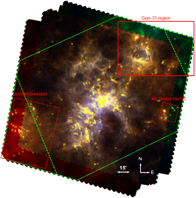
Figure 1: Herschel three color composite of the CNC maps at $70\,\mu$m (blue), $160\,\mu$m (green) and $250\,\mu$m (red). The yellow ’x’ mark the positions of our 642 Herschel point-like sources detected in at least two bands. The solid red box delineates the Gum 31 region that will be discussed in a separate paper. The two dashed red boxes delineate two clouds that are not part of the Carina Nebula and will also be discussed in a separate paper. The green polygon marks the region of the Carina Nebula that is also covered by the Spitzer IRAC maps. The two green dashed lines within the polygon mark the borders of the region for which our Spitzer photometry was obtained. Because the field-of-views of PACS and SPIRE are shifted to each other, there are regions that are only covered by one instrument, i.e. the red region in the south-west is only part of our SPIRE maps, and the green region in the north-east is only part of our PACS maps, respectively.

2 Observations and data reduction

We present Herschel far-infrared data of the CNC and complement it with Spitzer, 2MASS, and WISE data to obtain information in the shorter wavelengths. This allows the construction of SEDs over a wider wavelength regime than Herschel alone.

2.1 Herschel far-infrared maps

The Carina Nebula complex was observed by the Herschel satellite on December 26th, 2010. The maps obtained cover an area of $3.2\degr\times 3.2\degr$ corresponding to a physical region of 128 pc $\times$ 128 pc at the distance of the CNC, i.e. including the full extent of the complex. The CNC was simultaneously imaged in five different wavelengths, using the two on-board photometer cameras PACS (Poglitsch et al. 2010) at 70 and $160\,\mu$m and SPIRE (Griffin et al. 2010) at 250, 350, and $500\,\mu$m. Two orthogonal scan maps were obtained by mapping in the parallel fast scan mode with a velocity of $60\arcsec/{\rm s}$. The total observing time was 6.9 hours.

The data reduction was performed with the HIPE v7.0 (Ott 2010) and SCANAMORPHOS v10.0 (Roussel 2012) software packages. From level 0.5 to 1 the PACS data were reduced using the L1_scanMapMadMap script in the photometry pipeline in HIPE with the version 26 calibration tree. The level 2 maps were produced with SCANAMORPHOS with standard options for parallel mode observations, including turnaround data. The pixel-sizes for the two PACS maps at 70 and $160\,\mu$m were chosen as $3.2\arcsec$ and $4.5\arcsec$, respectively, as suggested by Traficante et al. (2011).

The level 0 SPIRE data were reduced with an adapted version of the HIPE script rosette_obsid1&2_script_level1 included in the SCANAMORPHOS package. Here the version 7 calibration tree was used. The final maps were produced by SCANAMORPHOS with standard options for parallel mode observations (turnaround data included). The pixel-sizes for the three SPIRE maps at 250, 350 and $500\,\mu$m were chosen as $6\arcsec$, $8\arcsec$ and $11.5\arcsec$, respectively. The angular resolutions of the maps are $5\arcsec$, $12\arcsec$, $18\arcsec$, $25\arcsec$, and $36\arcsec$ for the 70, 160, 250, 350, and $500\,\mu$m band, respectively. At the distance of the CNC this corresponds to physical scales from 0.06 to 0.4 pc.

2.2 Spitzer IRAC data

We retrieved the available data from the Spitzer Heritage Archive (PI: Steven R. Majewski; Program-ID: 40791) and assembled the basic calibrated data into wide-field ( $\approx 2.6\degr\times 3.0\degr$) mosaics that cover nearly the full extent of the Carina Nebula. As illustrated in Fig. 1, the Spitzer IRAC maps cover $\approx 87\%$ of the area of our Herschel maps. We performed point source detection and photometry in these IRAC mosaics, using the Astronomical Point source EXtractor (APEX) module of the MOsaicker and Point source EXtractor package (MOPEX; Makovoz & Marleau 2005), as described in Ohlendorf et al. (2012).

The entire Spitzer point-source catalog contains 569 774 objects; 548 053 of these are located in the area covered by our Herschel maps. The fluxes of the faintest objects in our point-source catalog range from $\approx 0.1$ mJy in the IRAC 1 and IRAC 2 maps, over $\approx 0.2$ mJy in IRAC 4, to $\approx 0.4$ mJy in IRAC 3. However, the detection limit is a strong function of location in the maps, because large parts of the mosaics are pervaded by very strong and highly inhomogeneous diffuse emission that reduces the local source detection sensitivity considerably.

In order to estimate typical values for the completeness limits of our Spitzer IRAC catalog across the field, we inspected the flux-distributions and determined the points where the flux histograms start to deviate from a power law-shape. This was found to occur at $\approx 1.1$ mJy for IRAC 1, $\approx 0.4$ mJy for IRAC 2, $\approx 1.2$ mJy for IRAC 3, and $\approx 1.2$ mJy for IRAC 4. These values can be regarded as typical average completeness limits; at locations of particularly bright [faint] nebulous emission the sensitivity can be considerably poorer [better].

We also retrieved a mosaic map of the CNC from the available Spitzer MIPS archive (PI: Jeff Hester; Program-ID: 20726). However, since a large fraction of the MIPS map is saturated by the very strong diffuse emission in the central parts of the Carina Nebula, no attempt was made to construct a photometric source catalog.

3 Construction of the catalog of point-like Herschel sources

3.1 Source detection and photometry

The point source detection and photometry in the five Herschel maps was carried out with CuTEx (Molinari et al. 2011), a software package developed especially for maps with complex background. It was developed and extensively tested by the Herschel infrared Galactic Plane Survey (Hi-GAL) team and is used for all point-source detection and photometry in the Hi-GAL project (Molinari et al. 2010). It calculates the second order derivatives of the signal map in four directions (x, y and their diagonals). Point-like sources produce steep brightness gradients compared to their surrounding background and can therefore be identified in the derivative of the map, i.e. curvature of the brightness distribution. Point sources should also have a similarly steep brightness gradient in all directions; this helps to distinguish them from elongated structures like filaments, which are a very prominent feature in the Herschel images. An image with an average of all four derivatives is shown for our SPIRE $250\,\mu$m map in Fig. 2. The differentiation dampens the background emission, enhancing the visibility of the point-like sources with respect to the original map. This allows to apply thresholding methods to detect the source peaks. A detection is considered significant when a certain curvature threshold is exceeded in all differentiation directions. For the photometry the routine assumes that the source brightness distribution can be approximated by a 2-dimensional elliptical Gaussian profile with variable size (FWHM) and orientation (position angle). To the varying background, the routine simultaneously fits an additional planar plateau at variable inclination and direction. This is done by cutting a limited fitting window around the source and estimating the background within this window. The fitted profiles are integrated to obtain the fluxes of the point-like sources.

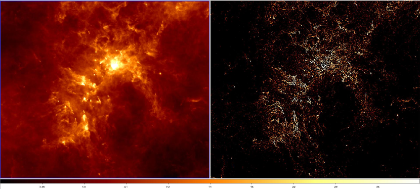
Figure 2: Second derivative image (on the right) of the SPIRE $250\,\mu$m map (on the left). Diffuse emission is dampened out and point-like sources are easily detectable by eye.

The best values for the detection parameters were chosen by visual inspection of the images. Our aim was that, on one hand, the faintest sources seen by eye were detected by the algorithm. On the other hand, care has been taken that nebulous extended structures and artifacts are excluded by the algorithm. We used a conservative approach that minimizes the number of spurious detections and excludes even slightly extended features such as nebular knots as far as possible. The parameters for the source detection step and the final number of point-like sources detected in each of the five bands are listed in Table 1.

For the photometry we set the /backgfit keyword in all maps to obtain a second order background fit. The other parameters were left at their default values. For some sources in the PACS $70\,\mu$m map, CuTEx assumed too small values for the PSF size. These cases were identified by visual inspection and this problem was solved by enlarging their PSF size values.

Table 1: Detection parameters and final source counts of CuTEx in our Herschel maps. The second, third and fourth column gives the final detection parameters used in CuTEx. The fifth column shows the number of detected point-like sources and the last one shows the number of sources in each band that are detected only in this band.

Band	pixel size	FWHM	beam size	PSFPIX	NPIX	thr	# Detections	# no detections in other bands
$[\mu$m]	[arcsec/pixel]	[arcsec]	[$\rm{arcsec}^{2}$]
70	3.2	5	28	1.56	4.0	9.5	454	168
160	4.5	12	148	2.70	4.0	8.5	552	72
250	6.0	18	361	2.98	4.0	6.5	650	104
350	8.0	25	708	3.13	4.0	6.0	471	36
500	11.5	36	1445	3.11	4.0	5.5	253	21

3.2 The Herschel point source catalog

Our final Herschel catalog was constructed in a very conservative way to provide a reliable and objective sample of point-like sources. As any source catalog based on maps with strong and highly spatially inhomogeneous background emission, our Herschel source lists for the individual maps may contain some number of spurious detections. In order to exclude spurious detections as far as possible, we included in our final catalog only those sources are detected independently in at least two different Herschel maps.
For this, the lists of point-like sources detected in each individual Herschel band were matched. The matching radius was chosen as $15\arcsec$ to account for the different angular resolution in the five bands. Starting with the shortest wavelength of $70\,\mu$m, i.e. the band with the best angular resolution, each detected source at this wavelength (parent source in the following) is checked for a match in every other Herschel band. A match is found if the source position lies within the matching radius of the parent source. If more than one match is found for the parent source within the matching radius, the closest is chosen. If, on the other hand, several parent sources have the same match in another band, this match is assigned to the closest parent source. This procedure is then repeated subsequently for the longer wavelengths. This procedure preserves for every source the coordinates derived from the map with the shortest wavelength in which it was detected, i.e. best angular resolution.
In the full area of our Herschel maps, 642 point-like sources were independently detected in at least two Herschel bands. The final statistics of this matching process can be found in Table 2.
The photometric catalog of these sources can be found in the appendix (Table LABEL:tbl:phot-fluxes-631).

While the use of such restrictive criteria leads to a very reliable catalog, it also automatically implies that a considerable number of true sources will be rejected, e.g. because small distortions of the PSF prevent an classification as “point-like” by the detection software. Our requirement of detection in at least two bands will also automatically remove many faint sources for which only the flux in the band closest to the peak of their spectral energy distribution is above the local detection limit. Therefore, single-band detections are not necessarily spurious sources.

We therefore produced a second catalog that lists the properties of these 500 additional Herschel source-candidates. It includes the objects detected by CuTEx in only one band, as well as a number of additional point-like sources that were found by visual inspection of the maps. It can be found in the appendix (Table LABEL:tbl:single-herschel-sources).

Our analysis in the rest of this paper remains, however, restricted to the sample of 642 point-like sources that were reliably detected in at least two bands.

Table 2: Final matching results all 642 point-like sources in the five Herschel bands.

# bands	# Sources
$\geq 2$	642
$\geq 3$	418
$\geq 4$	209
$=5$	75

3.3 Sensitivity limits of the Herschel point source catalog

According to the Herschel documentation, the theoretical $3\sigma$ sensitivity limits of PACS and SPIRE parallel mode observations in fast scan mode is about 40, 100, 25, 20, and 30 mJy in the 70, 160, 250, 350, and $500\,\mu$m band, respectively. These values are however, only theoretical limit for isolated point sources in regions without significant diffuse background. The true sensitivity limits in fields with strong and inhomogeneous background emission, as present in our maps of the Carina Nebula, are considerably higher. Due to the very strong spatial inhomogeneity of the cloud emission in our maps, the sensitivity cannot be precisely quantified by a single value.
Instead, we characterize it by two typical values, the optimum detection limit and the mode of the flux distribution.
The fluxes of the faintest detected sources are in the range $\approx 1-2$ Jy in our maps; this provides an estimate of the detection limit in regions without strong background emission.
The complex and bright background does not allow to determine a well-defined “completeness limit” for our maps. The modal values of the flux distributions are at $F_{\rm 70}\sim 10\leavevmode\nobreak\ {\rm Jy}$, $F_{\rm 160}\sim 15\leavevmode\nobreak\ {\rm Jy}$, $F_{\rm 250}\sim 10\leavevmode\nobreak\ {\rm Jy}$, $F_{\rm 350}\sim 10\leavevmode\nobreak\ {\rm Jy}$, and $F_{\rm 500}\sim 6\leavevmode\nobreak\ {\rm Jy}$. These values can serve as a rough proxy for the typical completeness limit across the field (i.e. the limit above which we expect most sources in the survey area to be detected as point-sources).

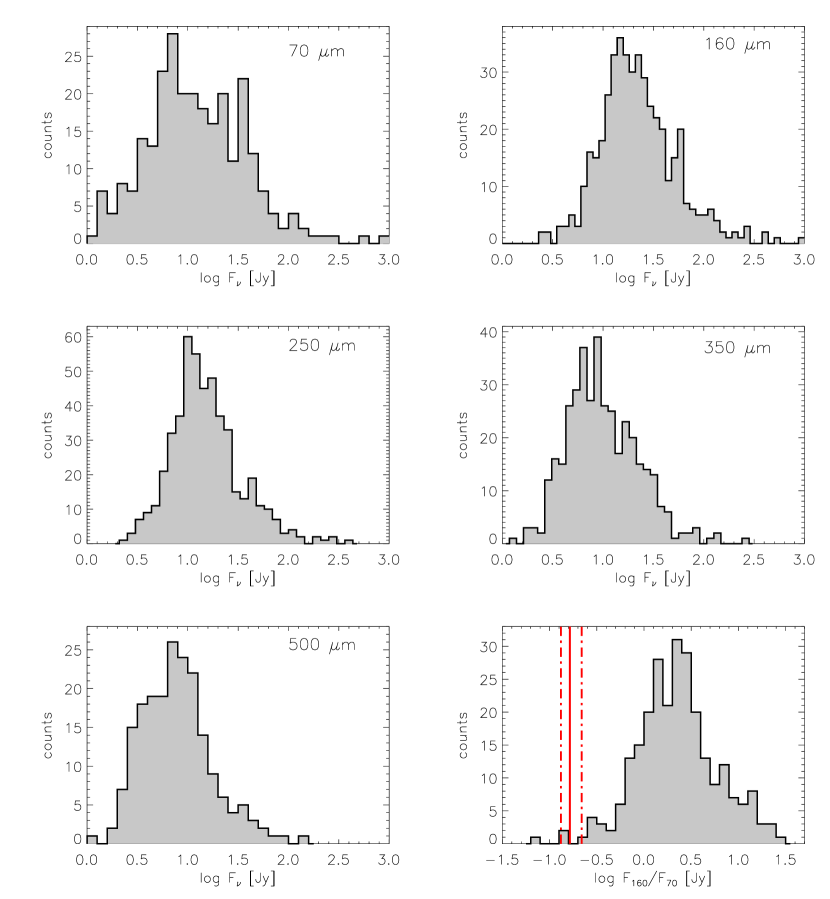
Figure 3: Flux histograms of the Herschel point-like sources in the CNC and Gum 31 for all five bands. In the bottom right corner a histogram of the flux ratio $F_{160}/F_{70}$ is shown. The solid red line marks the typical flux ratio for evolved stars which is $\sim 6$ as determined by Groenewegen et al. (2011). The two dot-dashed lines mark the $1\sigma$ interval of this ratio.

4 The nature of the Herschel point-like sources

4.1 Young stellar objects

The canonical model for the evolution of YSOs starts with the collapse of a pre-stellar core and proceeds through the embedded protostellar phase, where most of the mass is still in the circumstellar envelope, via a pre-main sequence star with circumstellar accretion disk to a ZAMS without (significant amounts of) circumstellar material. Observationally, these different phases can be traced by characteristic differences in the spectral energy distribution: according to the often used infrared classification scheme based on the slope of the near- to mid-infrared spectral energy distribution (Lada & Wilking 1984; Andre et al. 1993), Class 0 objects should represent early phases of protostars in collapsing cloud cores; Class I objects are more evolved protostars, but still embedded in a relatively massive, in-falling envelope; in Class II objects, the young star is nearly fully assembled, but still accreting from a circumstellar disk, while class III objects are pre-main sequence stars that have already dispersed their disks (see White et al. 2007).

Although we consider only “point-like” Herschel sources in this study, it is important to keep in mind that the relatively large PSF corresponds to quite large physical scales at the 2.3 kpc distance of the Carina Nebula. In the PACS $70\,\mu$m map, all objects with an angular [spatial] extent of up to $\approx 5^{\prime\prime}$ [11 500 AU = 0.056 pc] are compact enough to appear “point-like”. For the SPIRE $250\,\mu$m map, the corresponding numbers are $\approx 18^{\prime\prime}$ [41 400 AU = 0.20 pc]. This shows immediately that (pre-stellar) cloud cores, which have typical radii of $\la 0.1$ pc, cannot be (well) resolved in the Herschel maps and appear as compact “point-like” sources. This implies that YSOs in all the above mentioned stages can, in principle, appear as point-like sources in our Herschel maps. However, the possibility to detect an object in a specific stage depends strongly on its properties; as described below, many pre-stellar cores and embedded protostars will be easily detectable, while most of the more evolved pre-main sequence stars with disks should remain undetected.

Another possible problem could be externally illuminated nebular knots in the clouds. Such knots may be gravitationally unbound and thus never collapse to form stars, but if they are compact enough, they may nevertheless appear as point-like sources in our Herschel maps. Such knots constitute a general problem that concerns all Herschel maps, and is not specific to our study. From the Herschel data alone, it is not possible to reliably distinguish gravitationally unbound knots from bound cloud cores. However, the detection limits of our Herschel maps imply that all detected compact clouds must have substantial mass; at least one solar mass (see below). Minor inhomogeneities at the surface of large-scale clouds are thus unlikely to appear as detectable Herschel sources.

4.1.1 Herschel sensitivity to circumstellar matter

The far-infrared emission from a YSO is dominated by the thermal emission from circumstellar dust. The level of the far-infrared flux depends on several factors; the most important ones are (i) the amount of circumstellar material, (ii) the spatial distribution of this material, and (iii) the luminosity of the central YSO. Considering our Herschel detection limits of $\approx 1$ Jy, we used radiative transfer models to estimate the minimum values of the circumstellar mass and YSO luminosities that are required for a detection in at least two of the five Herschel bands.

Pre-stellar cores:

Radiative transfer simulations with the code and the dust model described in Preibisch et al. (1993), show that spherical pre-stellar cloud cores (i.e. no internal source of luminosity) with radii of 0.1 pc and temperatures of $T=20$ K can be detected for cloud masses of $\ga 2\,M_{\odot}$. Depending on the level of surface irradiation by nearby hot stars, this mass limit can decrease to $\ga 1\,M_{\odot}$.

Since the SEDs of pre-stellar cores drop steeply for wavelengths shorter than $\sim 100\,\mu$m, no emission is expected to be detectable in the Spitzer IRAC maps.

Ragan et al. (2012) presented radiative transfer models of starless cores and protostellar cores and investigated the detectability of these two different classes of objects. Their models showed that the SEDs of starless (i.e. pre-stellar) cores typically peak around $\approx 200-300\,\mu$m and drop very steeply towards shorter wavelengths. Their model fluxes at $70\,\mu$m (scaled to the distance of the CNC) are several orders of magnitudes below our detection limits.
Protostellar cores, on the other hand, have much stronger fluxes at PACS wavelengths. Guided by these results, we can thus use a detection at $70\,\mu$m as an indication for the protostellar nature of the source, whereas Herschel sources without $70\,\mu$m detection could be pre-stellar cores.
According to this, about 50% of our Herschel point-like sources are most likely protostellar objects.

Embedded protostars:

We performed radiative transfer simulations with the code and the dust model for protostellar envelopes described in Preibisch et al. (1993). We assumed the central protostar to be surrounded by a spherical dust envelope with a radius of 5000 AU and density power law $\rho(r)\propto r^{-1.5}$. In Table 3 we list for protostars of different mass (and corresponding luminosity) the minimum circumstellar envelope mass required for a detection in at least two of the five Herschel bands. As the luminosities of the protostars are highly time-dependent, the values listed were chosen considering the models of Siess et al. (1999), Palla & Stahler (1999), Hosokawa et al. (2010), and Klassen et al. (2012) and should be regarded as “typical” values.

Table 3: Minimum circumstellar envelope mass required for a detection in at least two of the five Herschel bands for protostars of different mass.

$M_{\rm protostar}$	$L_{\rm protostar}$	$\;\;\;\;M_{\rm env}$
$1\,M_{\odot}$	$30\,L_{\odot}$	$\ga 0.5\,M_{\odot}$
$2\,M_{\odot}$	$90\,L_{\odot}$	$\ga 0.25\,M_{\odot}$
$4\,M_{\odot}$	$200\,L_{\odot}$	$\ga 0.13\,M_{\odot}$
$6\,M_{\odot}$	$1600\,L_{\odot}$	$\ga 0.05\,M_{\odot}$
$10\,M_{\odot}$	$10\,000\,L_{\odot}$	$\ga 0.025\,M_{\odot}$
$20\,M_{\odot}$	$170\,000\,L_{\odot}$	$\ga 0.0125\,M_{\odot}$

The values for the minimum envelope masses drop strongly with increasing protostellar mass and luminosity. As the observed circumstellar masses for solar-mass Class 0 protostars in nearby star forming regions are typically around $1\,M_{\odot}$ (Jørgensen et al. 2009), i.e. a factor of two above our detection limit for $M_{\rm protostar}=1\,M_{\odot}$ protostars, we can expect to detect solar-mass protostars in the Carina Nebula in our Herschel maps. Less massive protostars ($M_{\rm protostar}<1\,M_{\odot}$) are generally not sufficiently luminous to produce far-infrared fluxes above our detection limits.

YSOs with circumstellar disks (T Tauri stars):

For more evolved YSOs, where much of the circumstellar material is in a circumstellar disks (but significant envelopes may still also be present), there are numerous possible spatial configurations for the circumstellar material. We therefore considered the Robitaille et al. (2006) YSO models, that contain YSOs with a wide range of different masses and evolutionary stages. We first selected from the grid of 20,000 models all those that represent YSOs with a specific stellar mass, and then determined which of these models would produce sufficiently strong fluxes for a detection in our Herschel maps and what the circumstellar (i.e. disk + envelope) mass of these models is. This analysis lead to the following results:

For $M_{\ast}=1\,M_{\odot}$ YSOs, most models with circumstellar mass $\ga 0.5\,M_{\odot}$ are above our Herschel detection limits; the lowest circumstellar mass of all detectable models is $\approx 0.1\,M_{\odot}$. For $M_{\ast}=3\,M_{\odot}$ YSOs, most models with circumstellar mass $\ga 0.1\,M_{\odot}$ are above the detection limits; the lowest circumstellar mass of all detectable models is is $\approx 0.05\,M_{\odot}$.

For $M_{\ast}=6\,M_{\odot}$ YSOs, most models with circumstellar mass $\ga 0.01\,M_{\odot}$ are above the detection limits; the lowest circumstellar mass of all detectable models is is $\approx 0.003\,M_{\odot}$.

For $M_{\ast}=10\,M_{\odot}$ YSOs, all models with circumstellar mass $\geq 0.0025\,M_{\odot}$ are above the detection limits.

To put these numbers in the proper context, we have to compare them to the observed circumstellar mass of YSOs in nearby star forming regions. For T Tauri stars, i.e. low-mass YSOs ($M_{\ast}\leq 2\,M_{\odot}$) with ages between $\sim 0.5$ Myr and a few Myr, disk masses of up to $M_{\rm disk}\sim 0.2\,M_{\odot}$ have been determined for some objects (Mann & Williams 2009), but the median disk masses are much lower, only around $M_{\rm disk}\sim 0.03\,M_{\odot}$ (Eisner et al. 2008). This implies that T Tauri stars with typical disk masses remain undetectable in our Herschel maps; we can only expect to detect a small fraction of the youngest T Tauri stars with particularly massive disks.

For intermediate-mass ($M_{\ast}\approx 2-10\,M_{\odot}$) YSOs, i.e. objects in the regime of Herbig Ae/Be stars, typical disk masses are about $0.03\,M_{\odot}$ (Boissier et al. 2011; Liu et al. 2011). Herbig Ae/Be stars with masses of at least $M_{\ast}\sim 4\,M_{\odot}$ are sufficiently luminous to be generally detectable in our Herschel maps.

4.1.2 Conclusions on the detection limit for YSOs

From these limits it is clear that we can detect only a small fraction of all YSOs in the Carina Nebula: YSOs with (proto-) stellar masses below $\approx 1\,M_{\odot}$ are usually undetectable (unless they would have exceptionally massive disks or envelopes).

According to the model representation of the field star IMF by Kroupa (2002), the number of stars with masses below $1\,M_{\odot}$ is about 10 times larger than the number of stars with masses above $1\,M_{\odot}$. This implies that we can detect only a few percent of the total young stellar and protostellar population as point-like sources in our Herschel maps.

4.2 Contamination

Although most of the far-infrared sources seen in our Herschel maps of the CNC will be YSOs, there may be some level of contamination by other kinds of objects. The two most relevant classes of possible contaminants are evolved stars and extragalactic objects.

4.2.1 Evolved stars

The source $\eta$ Carinae, which is a well known evolved massive star is of course excluded from our sample of YSOs. This object will be discussed in detail in Sec. 9.

Evolved stars experience high mass loss and are often surrounded by dusty circumstellar envelopes that produce strong excess emission at far-infrared wavelengths (e.g. Ladjal et al. 2010). The infrared SEDs of evolved stars can be quite similar to those of YSOs, and thus the nature of objects selected by criteria based on infrared excess alone is not immediately clear and can lead to ambiguities (e.g. Vieira et al. 2011).
In our case, the location of the vast majority of far-infrared sources inside (or close to) the molecular clouds clearly suggests that they are most likely YSOs. However, there is always the possibility that an unrelated background source behind the cloud complex may just appear to be located in the clouds.

As a first check for possible contamination of our sample by evolved stars, we used the SIMBAD database to search for AGB, SG, and RGB type stars within a $5\arcsec$ radius around each of our 631 Herschel point-like sources. The SIMBAD database lists 82 objects of the above mentioned type of object within the area of our maps, but none of these is associated with one of our Herschel point-like sources, suggesting that these known evolved stars in our field-of-view are too faint at far-infrared wavelengths to be detected in our Herschel maps.

In a further approach to quantify the possible level of contamination by evolved stars, we used the models of Marigo et al. (2008) to compute the expected far-infrared fluxes of asymptotic giant branch stars. Using the online tool we computed 10 357 stellar models. We then determined the far-infrared fluxes at the wavelengths of $60\,\mu$m and $160\,\mu$m for a model distance of $d\geq 2.5\leavevmode\nobreak\ \rm{kpc}$ (i.e., assuming that these evolved stars were located immediately behind the Carina Nebula). We found that only $\leq 147$ of the model AGB stars (i.e. $\leq 1.4\%$ of the total sample) would have far-infrared fluxes above our detection limits of $\sim 1$ Jy. This suggests that the probability to detect evolved stars located in the Galactic background behind the Carina Nebula is low.
Groenewegen et al. (2011) observed $\sim 150$ evolved stars with Herschel. They found the typical mean flux ratio of the PACS $70\,\mu$m and the PACS $160\,\mu$m flux for such stars to be $\approx 6.1\pm 1.5$. One can see that all but four of our sources have 160/70 ratios larger than this value, which is another indicator that the contamination of our sample of Herschel sources with evolved stars is very small.

4.2.2 Extragalactic contaminants

The possible level of extragalactic contamination can be determined from the results of Clements et al. (2010) who give galaxy number counts obtained from SPIRE observations for the first 14 deg² of the Herschel-ATLAS survey (Eales et al. 2010). The highest measured flux of any galaxy in this sample was 0.8 Jy, i.e. below our detection limit. Therefore, it appears very unlikely that our sample of point-like Herschel sources in the Carina Nebula contains extragalactic objects.

In conclusion, we find that the possible level of contamination must be very low. Most likely, all our Herschel point-like sources are YSOs associated to the Carina Nebula and will from now on be called YSO candidates.

5 Modeling the spectral energy distributions of the Herschel detected YSOs

In order to derive information about the properties of the Herschel detected YSOs, we assembled their spectral energy distributions (SEDs) over an as wide as possible wavelength range and compared them to radiative transfer models. For this analysis we focused on the Carina Nebula (see Fig. 1). The 67 objects associated with the distant molecular clouds at the eastern and western edge of our Herschel maps were excluded. Furthermore, the 92 sources in the region of the Gum 31 cloud will be analyzed in a separate study (Ohlendorf et al. 2012, A&A submitted). This leaves us with a total number of 482 Herschel point-like sources with fluxes detected in at least two bands.

Since the reliability of SED modeling depends strongly on the wavelength coverage, we considered only those objects from our Herschel catalog of point-like sources (see Sec. 3.2) that were detected in at least three Herschel bands and at least one Spitzer IRAC band. We performed a careful visual inspection of the Spitzer IRAC images to make sure that only those Herschel point-like sources that can be clearly identified by an apparently single Spitzer counterpart were included in the sample. Many Herschel point-like sources turned out to have no, unclear, or multiple Spitzer counterparts; these were rejected from the sample. As a further check, we also inspected our deep near-infrared VLT HAWK-I images (Preibisch et al. 2011b) for those Herschel sources that are located in the HAWK-I field-of-view and excluded two Herschel sources that turned out to be very compact star clusters. This procedure left us with a final sample of 80 reliable apparently single point-like sources with now fluxes in at least three Herschel bands and at least one Spitzer band. For 36 of these, we found apparently single counterparts in the 2MASS near-infrared images and added their near-infrared magnitudes as listed in the 2MASS point source catalog (Skrutskie et al. 2006) to the SED. Apparently single counterparts in the WISE All-Sky Data Release Catalog (Cutri et al. 2012) were found for 38 of these 80 Herschel sources and the 12 and $22\,\mu$m photometry was added. The complete sample of the 80 sources with all available fluxes used for the SED fitting can be found in Table LABEL:tbl:phot-fluxes-201.
The number of Herschel point-like sources in the CNC without a clear Spitzer counterpart, but at least three Herschel fluxes, is 241.

5.1 SED fitting with the Robitaille models

Robitaille et al. (2006) present a grid of 20,000 models of young stellar objects (YSOs) which were computed using a 2D radiative transfer code developed by Whitney et al. (2003). These models describe YSOs with a wide range of masses and in different evolutionary stages, from the early stages of protostars embedded in dense in-falling envelope, until the late pre-main sequence stage, when only a remnant disk is left. These models are characterized by numerous parameters describing the properties of the central object (e.g. mass, luminosity, temperature), the circumstellar envelope (e.g. outer radius, envelope accretion rate, opening angle of a cavity), and the circumstellar disk (e.g. mass, outer disk radius, disk accretion rate, flaring). For each model, SEDs are given for ten different inclinations, resulting in a total of 200,000 model SEDs.

To fit our sample of point-like sources, an IDL routine was implemented from the code of Robitaille et al. (2007) and Robitaille et al. (2006). The 80 point-like sources that have been analyzed have up to 14 fluxes from the five Herschel bands, the four Spitzer IRAC bands, the three 2MASS bands, and the WISE 12 and $22\,\mu$m bands. The distance was fixed to 2.3 kpc. The interstellar extinction was restricted to the range of $A_{\rm v}=[0...40]$ mag. Finally, an error of 10% was assigned to the 2MASS fluxes, an error of 20% to the Spitzer fluxes, and an error of 30% to the Herschel and WISE fluxes

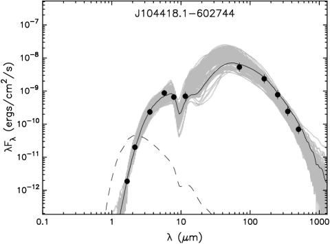
Figure 4: Example of a IR source with a good SED fit. The filled circles show the fluxes. The black line shows the best fit, and the gray lines show subsequent good fits with $\chi_{\nu}^{2}-\chi_{\nu,\rm best}^{2}<2$. The dashed line shows the stellar photosphere corresponding to the central source of the best fitting model, as it would look in the absence of circumstellar dust (but including interstellar extinction).

5.2 Stellar and circumstellar parameters of the YSO candidates

For 71 of the 80 sources, acceptable fits ($\chi_{\nu}^{2}<5$) were found. An example of such an acceptable fit is presented in Fig. 4 for source J104418.1$-$602744. Before considering the resulting best-fit values of the stellar and circumstellar parameters, we emphasize the well known fact that the results of SED fits can be highly ambiguous (e.g. Offner et al. 2012). Many of the stellar and circumstellar parameters are often poorly constrained because the models show a high degree of degeneracy (e.g. Men’shchikov & Henning 1997). We therefore restrict our analysis to a few selected parameters that can be relatively well determined from these fits. These are the total luminosity, the stellar mass, and the mass of the circumstellar envelope. Histograms for these three model parameters, as well as for the circumstellar disk mass, can be found in Fig. 5; the values and their individual uncertainties are listed in Table LABEL:tbl:model-param-ranges.

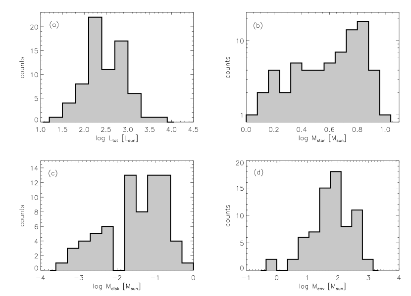
Figure 5: Histograms of the four model parameters obtained from the SED analysis for sources with an acceptable SED fit: Total luminosity (a), central stellar mass (b), circumstellar disk mass (c), and envelope mass (d).

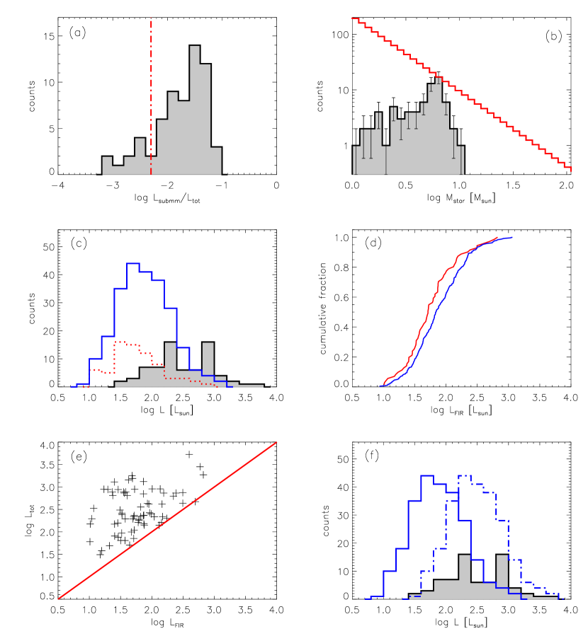
Figure 6: Total luminosities and central stellar mass of the Herschel YSOs. Top panels: (a) Ratio of the sub-mm luminosity (integrated SED for $\lambda\geq 350\,\mu$m) and the total luminosity obtained from the Robitaille models for all sources with an acceptable SED fit. The vertical dash-dotted red line marks the transition between Class 0 ($L_{\rm submm}/L_{\rm tot}\geq 0.005$) and Class I objects (see Andre et al. 1993). (b) Histogram of the stellar mass. The solid red line shows the IMF with a slope of $\gamma=-1.35$. Middle panels: (c) Histogram of the total luminosity obtained from the Robitaille models for sources with an acceptable SED fit (gray histogram). Overploted are the integrated far-infrared luminosity $L_{\rm int,FIR}$ of all sources with an acceptable SED fit (dotted red histogram), and the integrated far-infrared luminosity of all Herschel point-like sources in the CNC with fluxes detected in minimum three bands and without an SED fit (solid blue histogram). (d) Cumulative distribution function of the integrated far-infrared luminosity of all sources with an acceptable SED fit (red pluses), and the integrated far-infrared luminosity of all Herschel point-like sources in the CNC with fluxes detected in minimum three bands and without an SED fit (blue crosses). Bottom panels: (e) Total luminosity obtained from the Robitaille models versus the integrated far-infrared luminosity for all sources with an acceptable SED fit. The solid red line marks a ratio of 1. (f) Same as (c), but now with the distribution of the integrated far-infrared luminosity of all Herschel point-like sources in the CNC with fluxes detected in minimum three bands and without an SED fit (solid blue) multiplied by the median value of $L_{tot}/L_{FIR}$ for YSOs with SED fit (dash-dotted blue).

Total luminosity:

The total luminosity is relatively well determined by the amplitude of the SED, because the Herschel bands cover the broad far-infrared peak of the SED quite well. The total luminosities of the YSOs derived from the fits range from $\approx 30\,L_{\odot}$ to $\approx 5300\,L_{\odot}$. The lower boundary is a result of the detection limit. The rather moderate value of the upper boundary, however, will lead to interesting conclusions about the currently forming stellar population, as will be discussed below.

(Proto-) stellar mass:

The (proto-) stellar masses are rather tightly related to the total luminosities in these models. The derived values range from $1\,M_{\odot}$ up to $\approx 10\,M_{\odot}$. The lower boundary is again the result of the detection limit and agrees well with the estimates discussed above. The upper boundary, however, is surprisingly low, given the fact that the Carina Nebula contains at least 70 stars with masses of well above $20\,M_{\odot}$, including numerous very massive ($M\ga 50\,M_{\odot}$) stars. The derived mass distribution for the Herschel detected YSOs suggests that the currently forming generation of stars in the CNC is restricted to intermediate- and low-mass stars, but does not seem to form stars as massive as present in large numbers in the slightly older population of optically visible stars. We note that the lack of high-mass YSOs is not an artifact of the model grid: the Robitaille grid contains objects with masses up to $50\,M_{\odot}$. A more detailed discussion of these aspects will be presented in Sec. 6.

Circumstellar disk mass:

The disk mass is not a very well constrained parameter, because there are large ambiguities with the envelope mass. Nevertheless, we note that the best-fit values range between $0.0004\,M_{\odot}$ and $0.6\,M_{\odot}$.

Envelope mass:

The rather high values we find for the envelope masses (between $10\,M_{\odot}$ and $1000\,M_{\odot}$) confirm the expectation that most of the Herschel detected YSOs are protostars still embedded in rather massive envelopes.

5.3 Sub-mm luminosities of the point-like sources

The observational definition of protostars is based on the ratio of the sub-mm luminosity to the total luminosity of a YSO. Objects with fractional sub-mm luminosity of at least $L_{\rm submm}/L_{\rm tot}\geq 0.005$ are defined as “Class 0 protostars” (Andre et al. 1993). Since this ratio requires knowledge of the total luminosity, we can only apply it to the YSO in the SED fit sample.

We calculated the sub-mm luminosity for all sources with an SED fit, integrating the SED for $\lambda\geq 350\,\mu$m, which in this case resulted in the sum over the two longer SPIRE bands at 350 and $500\,\mu$m: $L_{\rm submm}=F_{350}\times{\rm d}\nu_{350}\,+\,F_{500}\times{\rm d}\nu_{500}$ with $F_{\nu}$ the flux density and ${\rm d}\nu$ the width of the band filter. The resulting values are shown as a histogram in Fig. 6a. Fifty-three of the 71 objects, i.e. 75%, can be classified as Class 0 protostars.

The fraction of Class 0 protostars among the 402 Herschel YSOs for which no clear Spitzer counterparts could be found is most likely even larger (because the absence of a Spitzer counterpart suggests the object to be a pre-stellar core or a very young protostar). This demonstrates that the sample of Herschel-detected YSOs traces the extremely young population of currently forming stars; these objects are systematically younger than the YSO population revealed by the Spitzer observations (Smith et al. 2010b; Povich et al. 2011).

5.4 Luminosities of the YSOs without SED fit

The 71 objects with acceptable SED fits represent only 15% of the total number of Herschel point-like sources in the analyzed area of the Carina Nebula. For most of the remaining sources, no clear counterparts at shorter wavelengths could be found. Some of these objects may be pre-stellar cores, but some could also be protostars with very dense envelopes that prevent their detection in the Spitzer maps.

The only information that can be derived about these objects from the present data is the far-infrared luminosity, integrated over the wavelength range covered by our Herschel data. We computed these values as the sum of the observed fluxes multiplied by the bandwidth. The resulting far-infrared luminosities are shown in the histogram in Fig. 6c. The median of this distribution is $69.2\,L_{\odot}$ and the maximum is $1150\,L_{\odot}$.

In order to investigate how similar or different the Herschel-detected objects without clear Spitzer counterparts are with respect of those that have clear Spitzer counterparts, we compare the far-infrared luminosities of these two groups in Fig. 6c. Their cumulative distribution functions are shown in Fig. 6d. A Kolmogorov-Smirnov test gives a probability of $P_{0}=0.08$ that both samples are drawn from the same parent distribution. This indicates that the far-infrared luminosities of the sources with a clear Spitzer counterpart are slightly systematically lower (by about 30%) than those without Spitzer counterpart. However, the statistical significance of this difference is marginal, and we thus can assume that also the distribution of total luminosities in the full sample of Herschel-detected objects should be similar to those of the objects with SED fit.

In Fig. 6e we compare the far-infrared luminosities of the objects with SED fit to their total luminosities. The median value for the ratio $L_{\rm tot}/L_{\rm FIR}$ of this sample is 4.25. Multiplying the distribution of far-infrared luminosities of the objects without SED fit by this factor can thus give us a (crude) estimate of the distribution of their total luminosities. The resulting distribution, based on this simple extrapolation factor, is shown in Fig. 6f. One can see that the extrapolated distribution of total luminosities agrees reasonably well with the distribution of total luminosities for the objects with SED fits. The most important point is that the extrapolated total luminosities are again restricted to values below $\la 5000\,L_{\odot}$.
At this point we note that Herschel sources without Spitzer detections are expected to have a systematically lower $L_{\rm tot}/L_{\rm FIR}$ than sources with Spitzer detections. Although there are substantial uncertainties in this extrapolation, these results suggest that there is no significant number of YSO with total luminosities exceeding $10\,000\,L_{\odot}$, i.e. the lower limit for high-mass YSOs.

6 The mass function of the Herschel detected YSOs

6.1 The apparent deficit of massive YSOs

Our SED modeling suggests that all of the analyzed Herschel YSOs in the CNC are YSOs of low- or intermediate mass, $M_{\ast}\la 10\,M_{\odot}$. The result of a lack of high-mass YSOs is also corroborated by the fact that none of the Herschel detected YSOs in our full sample has a luminosity of more than $10^{4}\,L_{\odot}$ (which is the lower boundary for high-mass YSOs). If a massive YSO with such a high luminosity existed in the Carina Nebula, there is no reason why it should not be detected as a very prominent and bright far-infrared source in our Herschel maps.

The absence of massive YSOs is also supported by the lack of hyper-and ultra-compact H II regions. This is quite remarkable, given the large number of high-mass stars in the young stellar populations in the Carina Nebula: the compilation of Smith (2006) lists 70 O-type stars (with stellar masses $\geq 20\,M_{\odot}$), among which there are 18 stars with stellar masses $\geq 50\,M_{\odot}$.

To illustrate the lack of massive stars among the Herschel detected YSOs, we compare in Fig. 6b their mass distribution to the shape of the field-star IMF. For masses above $\approx 6\,M_{\odot}$, the observed distribution of YSO masses drops much more quickly with increasing mass than the field star IMF and reveals an apparent deficit of stars $M_{*}\ga 10\,M_{\odot}$.

6.2 Detection limits and biases

A similar result was obtained by Povich et al. (2011) from their analysis of their Spitzer selected YSO sample: they also found no YSO with masses above $M_{\ast}\approx 10\,M_{\odot}$. They interpreted this as an effect of the infrared-excess selection of their sample: since massive stars disperse their disks on shorter timescales than lower mass stars, they display infrared excesses (and thus are detectable via infrared excess emission) for a shorter period of time. The “canonical” disk lifetime for solar-mass YSOs is $\sim 2-3$ Myr (see Muench et al. 2007; Fedele et al. 2010), i.e. considerably longer than the $0.1-1$ Myr disk lifetime determined for intermediate-mass YSOs (Hernández et al. 2005; Povich et al. 2011; Roccatagliata et al. 2011; Sandell et al. 2011). As the Spitzer data are sensitive enough to detect several Myr old solar-mass YSOs with rather low disk masses, this is a valid explanation for the lack of massive objects in the Spitzer excess-selected YSO sample.

For our Herschel selected sample, the situation is different, because the detection limits are much more restrictive. The relevant timescale is not the disk lifetime, but the timescale, for which a YSO still has a sufficient amount of circumstellar material to produce enough far-infrared emission to be detectable. As discussed above in Sec. 4.1.1, solar-mass YSOs can only be detected in our Herschel maps during their early protostellar phase or as long as they have exceptionally massive disks. The typical timescale for which such solar-mass YSOs are detectable is thus the duration of the protostellar phase, i.e. about $0.1$ Myr (see Evans 2011) which is much shorter than the “canonical” disk lifetime. Another important aspect is the strong dependence of the minimum required circumstellar mass for a Herschel detection on the luminosity (and thus the mass) of the YSO. As determined above, the minimal required circumstellar mass decreases from $\sim 0.5\,M_{\odot}$ for $M_{\ast}=1\,M_{\odot}$ YSOs, via $\sim 0.01-0.05\,M_{\odot}$ for $M_{\ast}=6\,M_{\odot}$ YSOs to $\sim 0.002-0.01\,M_{\odot}$ for $M_{\ast}=20\,M_{\odot}$ YSOs. This leads to a situation where the period of time, during which the YSOs are detectable for Herschel, is not decreasing with increasing stellar mass.

For high-mass ($M\geq 10\,M_{\odot}$) stars, the lifetime of circumstellar material is not well known, since the details of the formation mechanism of high-mass stars are still not well understood (Zinnecker & Yorke 2007). From an observational point of view, protostars of $\leq 20\,M_{\odot}$ are often surrounded by disks containing several solar masses of circumstellar matter (e.g. Patel et al. 2005; Cesaroni et al. 2007). For higher protostellar masses, the situation is still unclear since no good examples of proto O-stars have been found so far. We thus have to consider the results of numerical simulations of massive star formation. The calculations of Yorke & Sonnhalter (2002), Krumholz et al. (2009), Kuiper et al. (2011), and Klassen et al. (2012) showed that the forming massive stars are surrounded by considerable amounts of circumstellar matter (of the order of a few solar-masses, i.e. well above the minimum circumstellar mass required for a Herschel detection) for at least about 50 000 – 100 000 years. This suggests that the period of time during which YSOs are detectable for Herschel is not a strong function of YSO mass. This agrees and is supported by the estimate of $\approx 10^{5}$ yr for massive YSO lifetimes by Mottram et al. (2011).

6.3 Quantification of the massive YSO deficit

In order to quantify the deficit of massive YSO, we consider the number of YSOs in the $[5-7]\,M_{\odot}$ mass range. This range covers the peak of the observed YSO mass function, and its lower end is high enough not be affected by incompleteness of detection. Our sample of Herschel-detected YSOs with acceptable SED fits contains 31 objects in the $[5-7]\,M_{\odot}$ mass range.

According to the model representation of the field star IMF by Kroupa (2002), the ratio of the number of stars in the $[10-100]\,M_{\odot}$ mass range to those in the $[5-7]\,M_{\odot}$ mass range is 1.09.

Therefore, assuming a field-star IMF, the expected number of YSOs in the $[10-100]\,M_{\odot}$ mass range would be $\approx 34$.
Even if we (conservatively) assume that the period of time during which the massive YSO are detectable for Herschel is a factor of three shorter than those of the $[5-7]\,M_{\odot}$ YSOs, the expected number of high-mass YSOs would be about 11, whereas the actually observed number is zero.

It is highly unlikely that the non-detection of such objects is a statistical effect, since the Poisson probability to detect no object if the expectation value is 11, is $e^{-11}=1.7\times 10^{-5}$.

We can thus conclude that the mass distribution of the currently forming generation of stars detected by Herschel is different from the IMF of the optically visible population of the several Myr old stellar population in the Carina Nebula. This difference seems to be related to the fact that nearly all the clouds in which star formation is currently proceeding have too low densities and masses to allow the formation of very massive stars (see discussion in Preibisch et al. 2011c).

7 Estimates for the size of the protostellar population and the star formation rate

Since our Herschel maps cover the full spatial extent of the Carina Nebula Complex, the results can be used to estimate the total size of the protostellar population. Considering the Carina Nebula Complex (including the area around Gum 31), but excluding the 67 objects in the distant molecular clouds at the eastern and western edge of our maps, the total number of YSOs detected as Herschel point-like sources is 574. Applying the criteria from Ragan et al. (2012) for the distinction of pre- and protostellar cores, we consider these 267 Herschel point-like sources with a $70\,\mu$m detection to be YSO (whereas the Herschel sources without a 70 m detection may be pre-stellar cores). As determined in Sect. 5.3, we can further assume that about 75% of these 267 Herschel-detected YSOs are Class 0 protostars. Hence the number of Herschel-detected protostars in the entire CNC (including the Gum 31 region) is 200. To estimate the total number of protostars, we need an estimate of the completeness of our sample. For this, we use the modal value of the $70\,\mu$m flux distribution ($\approx 6$ Jy; see Fig. 3) as an approximation of the detection completeness. In order to find the corresponding protostellar mass limit, we again consider the Robitaille models. We first selected from this grid models representing YSOs with a specific stellar mass and additionally fulfill the condition that their circumstellar (i.e. disk+envelope) mass is at least half of the stellar mass (this restricts the selection to protostellar objects). Then we determined the stellar mass for which at least 50% of the models in these samples show $70\,\mu$m fluxes above the 6 Jy limit. The resulting estimate of the completeness limit is about $2\,M_{\odot}$. Assuming a Kroupa IMF, the number of stars in the $0.1-2\,M_{\odot}$ range is approximately 20 times larger than the number of stars above $2\,M_{\odot}$. Since the number of Herschel-detected protostars in the CNC with $70\,\mu$m fluxes above the model value of 6 Jy is 144, our estimate of the total protostellar population is $\approx 144\times 20=2880$.
If these protostars formed over a period of 100 000 years (i.e., the estimated lifetime of the protostellar phase), this implies a star formation rate of about 0.029 stars per year. Using the mean stellar mass of $0.6\,M_{\odot}$ (according to the Kroupa field star IMF for the mass range $0.1-100\,M_{\odot}$), the star formation rate of the CNC is then $0.017\,M_{\odot}/\rm{yr}$.
It is interesting to compare our result to the star formation determinations by Povich et al. (2011). They derived a lower limit of $\ga 0.008\,M_{\odot}/\rm{yr}$ for the recent star formation rate, averaged over the past 2 Myr, based on their analysis of a Spitzer-selected sample of YSOs. For the average star formation rate over the past 5 Myr they derived $0.010-0.017\,M_{\odot}/\rm{yr}$. For a meaningful comparison to our estimate, we have to take into account that the area Povich considered is restricted to the central 1.4 square-degrees of the Carina Nebula, whereas our Herschel sample covers the entire CNC, including the Gum 31 region. Considering these different areas, we find that 76% of our Herschel point-like sources are in the area that also was studied by Povich. Scaling our SFR estimate for the entire CNC by this factor, the resulting rate of 0.013 for the central area agrees very well with the rates determined by Povich.
We note that this good agreement of two completely independent estimates is encouraging. It also suggests that the star formation activity in the CNC remained approximately constant in the time from several Myr ago until today.

8 Spatial distribution of the YSO candidates

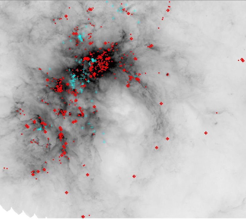
Figure 9: Herschel PACS $70\,\mu$m image of the CNC with square root intensity scale. The positions of the OB stars from Smith (2006) are marked with cyan crosses. Positions of the Herschel point-like sources are marked with red squares. The positions of all 80 YSOs with SED fits are marked with red diamonds. Note that their distribution is concentrated on the cloud edges.

The spatial distribution of the YSO candidates is shown in Fig. 9. It is important to note that all clouds in the CNC are transparent at all Herschel wavelengths. This implies that cloud extinction is not an issue and all (sufficiently luminous) YSOs should be detectable at all locations in our Herschel maps.

Most Herschel YSO candidates are located in the central regions of the Carina Nebula and the South Pillars region. In the northern part of the field, the source density is considerably lower. A particularly interesting result is that the source density does not follow the distribution of cloud masses. The most prominent example for this effect is the particularly massive and dense Northern Cloud (just to the west of the stellar cluster Tr 14): although this cloud has a mass of about $50\,000\,M_{\odot}$ (Preibisch et al. 2012), just about 30 YSO candidates are seen in the dense regions of the cloud. Most of these are located at the eastern edge, where the cloud is strongly irradiated by the numerous massive stars in the Tr 16 and Tr 14 clusters.

Also in the other regions, the Herschel YSOs are preferentially located at the surfaces of irradiated clouds or in narrow filaments. This shows that the spatial distribution of the Herschel YSOs (i.e. the current star formation activity) does not follow the distribution of cloud mass, but is largely restricted to locations of strong irradiation, i.e. the edges of irradiated clouds.

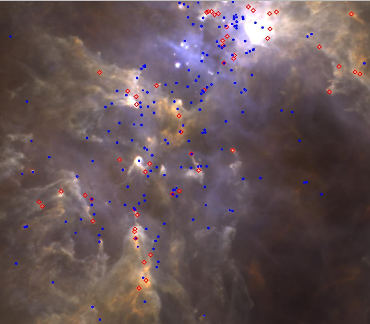
Figure 10: Same color composite image as in Fig. 1 of the South Pillars region. Positions of the YSO candidates are again marked with red diamonds. The blue circles represent the class 0 and class I YSOs from the PCYC catalog by Povich et al. (2011). Note that the region around $\eta$ Car lacks Spitzer YSOs because of the nebulosity caused by itself.

In order to investigate this further, we show in Fig. 10 a part of the central Carina Nebula and the Southern Pillars and compare the spatial distribution of the Herschel YSO candidates to the one of the Spitzer YSO candidates from the Pan Carina YSO Catalog (PCYC) catalog (Povich et al. 2011).
These two samples should represent two different populations of young objects, where the Herschel sample is dominated by very young, deeply embedded protostellar objects (with ages of about $\la 0.1$ Myr), while the PCYC sample should mostly consist of slightly older, more evolved young stars (Class I sources and T Tauri stars). Fig. 10 shows that most Herschel YSO candidates are located near the irradiated surfaces of clouds and pillars, whereas the Spitzer selected YSO candidates often surround these pillars.

This characteristic spatial distribution of the young stellar populations in different evolutionary stages agrees very well with the idea that the advancing ionization fronts compress the clouds and lead to cloud collapse and star formation in these clouds, just ahead of the ionization fronts. Some fraction of the cloud mass is transformed into stars (and these are the YSOs detected by Herschel), while another fraction of the cloud material is dispersed by the process of photo-evaporation. As time proceeds, the pillars shrink, and a population of slightly older YSOs is left behind and revealed after the passage of the ionization front. This result provides additional evidence that the formation of these YSOs was indeed triggered by the advancing ionization fronts of the massive stars as suggested by the theoretical models (see Gritschneder et al. 2010; Smith et al. 2010b).

9 The far-infrared spectral energy distribution of $\eta$ Carinae

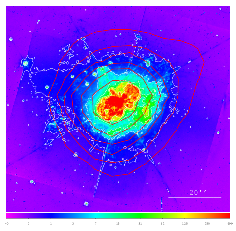
Figure 7: HST/WFPC2 image (data set hst_9226_01_wfpc2_f658n_wf) of $\eta$ Carinae obtained through the narrow-band filter F658N. The image is displayed with a logarithmic intensity scale in order to show the rather faint nebular features of the outer ejecta. The thin white contour lines also highlight the structure of the optical nebula. The thick red contours trace the Herschel $70\,\mu$m band emission. The contour levels start at 3.125 Jy/pixel and increase by a factor of 2 up to the 200 Jy/pixel level.

The Luminous Blue Variable $\eta$ Carinae (see Davidson & Humphreys 1997) is one of the most luminous $(L_{\ast}\geq 5\times 10^{6}\,L_{\odot}$) massive stars in our Galaxy. Despite numerous observations in all wavelength regimes, the exact nature and evolutionary state of this object remain as yet elusive (Davidson & Humphreys 1997). The object seems to be a binary with a period of 5.5 years, and the extremely strong stellar winds with a mass loss rate of about $\dot{M}\sim 10^{-3}\,M_{\odot}/{\rm yr}$ cause very strong shocks and resulting high-energy radiation from the wind-wind collision zone (see, e.g. Groh et al. 2010; Farnier et al. 2011). $\eta$ Car displays strong variability in almost all spectral regimes. In the optical, it once represented the second brightest star on the sky, but faded by more than eight magnitudes between 1850 and 1880. During the last three decades, it brightened by several magnitudes (Martin et al. 2006; Smith & Frew 2011). Strong X-ray variability is seen as a result of dynamical changes in the wind collision zone (Corcoran et al. 2010). The observed near-infrared variability is probably related to the episodic formation of dust grains within compressed post-shock zones of the colliding winds (Smith 2010).

Our Herschel images show a very bright and prominent compact source at the position of $\eta$ Car. The far-infrared emission originates from the circumstellar dust envelope around $\eta$ Car. The famous bipolar Homunculus Nebula is thought to be the result of the “Great Eruption“ in the 1840’s (see Smith et al. 1998; Currie & Dowling 1999; Morse et al. 2001; Smith 2005; Artigau et al. 2011; Davidson & Humphreys 2012). The total dust + gas mass in the bipolar nebula and a dense equatorial torus in the Homunculus is estimated to be about $15-20\,M_{\odot}$ (Morris et al. 1999; Smith et al. 2003). The angular diameter of the optically bright parts of the Homunculus Nebula as seen in the HST images is $18^{\prime\prime}\times 11^{\prime\prime}$ (long axis $\times$ short axis). The bright mid-infrared emission, measured in an $18\,\mu$m image obtained with the Magellan Telescope by Smith et al. (2003), has the same extension. This size scale implies that the Homunculus Nebula should be marginally resolved in our Herschel PACS maps, but unresolved in the SPIRE maps. However, the Homunculus Nebula is surrounded by the so-called “outer ejecta”, a collection of numerous filaments, shaped irregularly and distributed over an area of $\approx 1^{\prime}\times 1^{\prime}$ (Weis 2004); the dust in these outer parts could also contribute to the far-infrared emission.

In Fig. 7 we show the contours of the Herschel $70\,\mu$m emission on an optical HST WFPC2 image taken through the narrow-band filter F658N (data set ${\rm hst\_9226\_01\_wfpc2\_f658n\_wf}$, observed on 2001-06-04, exposure time 923.33 sec) that shows the Homunculus Nebula and the surrounding outer ejecta. A two dimensional Gaussian fit to the $70\,\mu$m emission in (using the command Pick Object in GAIA) yields a FWHM size of $18.1^{\prime\prime}\times 14.9^{\prime\prime}$, which is clearly larger than the FWHM size of $10^{\prime\prime}\times 10^{\prime\prime}$ measured for several isolated point-like sources in the same map. The measured direction of elongation is along a position angle of $33\degr$, well consistent with the orientation of the Homunculus Nebula.

Due to the good angular resolution of our Herschel maps, the compact far-infrared emission around $\eta$ Carinae can be well separated from the surrounding background. We performed aperture photometry using circular apertures with radii of $45\arcsec$ for the 70, 160, and $250\,\mu$m bands, $50\arcsec$ for the $350\,\mu$m band, and $72\arcsec$ for the $500\,\mu$m band; these apertures are large enough to include not only the Homunculus Nebula, but also possible contributions from the “outer ejecta” (which extend up to radial distances of $30\arcsec$ from $\eta$ Car). The fluxes derived in this way are 6685 Jy, 1163 Jy, 302 Jy, 138 Jy and 72 Jy, for the 70, 160, 250, 350, and $500\,\mu$m band, respectively.

The resulting, very high, PACS fluxes have to be treated with caution, since they are clearly in the non-linear regime ($\geq 200$ Jy) of the instrument. The $70\,\mu$m flux, and also the $160\,\mu$m flux (although to a lower level), is also affected by readout saturation, which starts at 200 Jy for PACS $70\,\mu$m and 1125 Jy for PACS $160\,\mu$m. Since there is no experience with possible corrections for non-linearity and saturation at such high flux levels (Herschel Helpdesk, priv. comm.), the obtained PACS fluxes can only be used as lower limits to the true fluxes. For SPIRE, the much lower measured source fluxes are below the instrumental saturation level (Herschel Helpdesk, priv. comm.). As an additional check, we inspected the raw data (timelines and masks), but found no indications for truncations because of ADC saturation. We thus can assume the derived SPIRE fluxes of $\eta$ Car to be reliable.

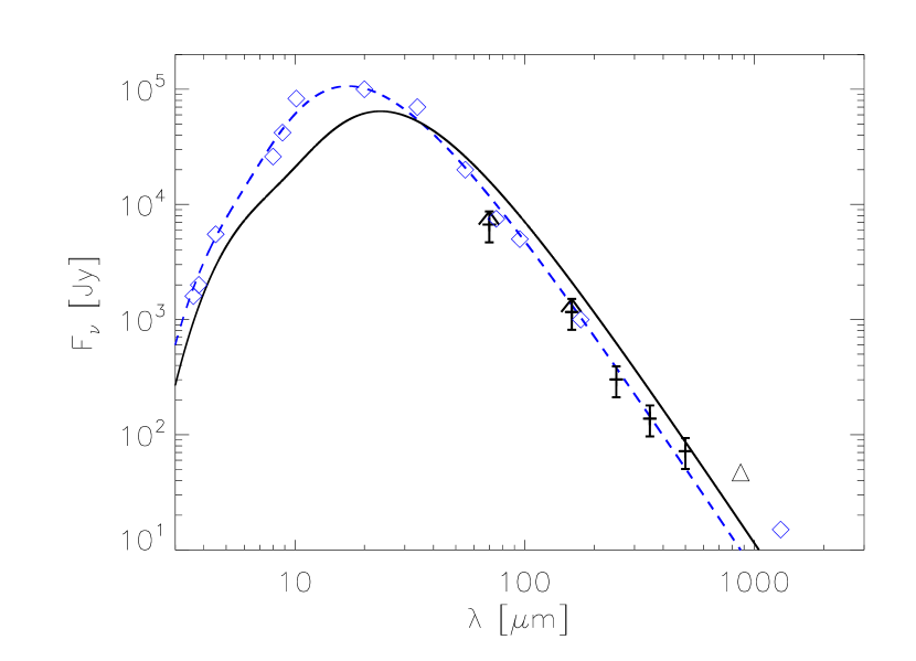
Figure 8: Spectral Energy Distribution of $\eta$ Carinae. The black crosses show our Herschel fluxes. The $70\,\mu$m and $160\,\mu$m PACS fluxes represent upper limits. The black triangle shows our LABOCA $870\,\mu$m flux determined in Preibisch et al. (2011c). The blue diamonds are the data from Cox et al. (1995). The dashed line represents the sum of two modified Planck spectra for dust temperatures of 210 K and 430 K from the model of Cox et al. (1995), the solid line the sum of three Planck spectra for dust temperatures of 140 K, 200 K, and 400 K from the model of Smith et al. (2003). We note that for wavelengths above $\geq 500\,\mu$m the SED gets dominated by free-free emission of the Homunculus nebula and the radiation originating in the ionized stellar wind of $\eta$ Car.

Several mid- to far-infrared observations of $\eta$ Car have been presented in the literature, and the SED was often fitted by the sum of modified black-body curves for different dust temperature. In Fig. 8, we compare our Herschel fluxes to the measurements and SED model described in Cox et al. (1995). Our Herschel SPIRE fluxes are well consistent (within the $1\sigma$ uncertainty range) with this SED model prediction. In their SED model Cox et al. (1995) use the far-infrared fluxes reported by Harvey et al. (1978). They were obtained with the Kuiper Airborne Observatory in March 1977, i.e. 33.8 years before our Herschel observations. This good agreement would seem to suggest long-term stability of the thermal dust emission.

Morris et al. (1999) presented the $2\,\mu$m to $200\,\mu$m spectrum of $\eta$ Car as obtained in January 1996 with the Infrared Space Observatory SWS and LWS spectrometers. They found considerably higher far-infrared fluxes than the values of Harvey et al. (1978) and attributed “these differences as a matter of calibration of the older photometry, based on observations of Uranus as the photometric standard”.

We show in Fig. 8 the SED fit to the ISO spectrum derived by Smith et al. (2003), which is based on the sum of three modified Planck functions with temperatures of 140 K, 200 K, and 400 K. Compared to this SED model, our Herschel SPIRE fluxes are considerably lower: The observed $250\,\mu$m flux (302 Jy) amounts to just 50% of the level expected from the model SED based on the ISO spectrum (624 Jy). In the $350\,\mu$m band, the observed flux (138 Jy) is just 57% of the level expected from the model SED based on the ISO spectrum (241 Jy). Even in the $500\,\mu$m band, where the SED already contains a significant contribution from free-free emission above the thermal dust emission, the observed flux of 72 Jy is lower than the expectation from the model SED based on the ISO spectrum (86 Jy). These discrepancies suggest a considerable decrease of the far-infrared luminosity, by about a factor of two, over the last 15 years.

What could be the reason for such a drop in the far-infrared emission? The first possibility we consider here is the dynamical expansion of the envelope. It is known that the material in the Homunculus moves outwards at about 600 km/s. With increasing distance from the illuminating source, the dust is less strongly heated, thus cools down and will produce less far-infrared emission. Within 15 years, the outer edge of the Homunculus (where the rather cool dust that emits most far-infrared radiation is located) moves from a radial angular distance of about $9^{\prime\prime}$ to about $10^{\prime\prime}$, and this implies that the heating of the dust at the outer edge of the Homunculus (due to the irradiation from the central binary system) drops by about 20%. This effect is too small to explain a drop of the far-infrared emission by a factor of $\sim 2$.

A more promising explanation may be dynamical changes in the structure of the inner dust envelope around $\eta$ Car. In the optical band, the brightness of $\eta$ Car increased by several magnitudes during the last $\sim 30$ years (see Fernández-Lajús et al. 2009; Gomez et al. 2010; Smith & Frew 2011). This increasing optical brightness suggests that the inner envelope, that enshrouds the central star, is currently opening up (Martin et al. 2006), and a larger fraction of the stellar optical and UV radiation, that was previously absorbed within the nebula and thus heated the dust, is now able to leave the system. As a consequence, the fraction of the stellar radiation that is absorbed and heats the dust in the envelope decreases. This finally leads to lower levels of thermal dust emission at far-infrared wavelengths and might explain the apparent drop of the far-infrared fluxes.

10 Summary and Conclusions

Our Herschel far-infrared ($70-500\,\mu$m) maps of the Carina Nebula complex revealed 642 reliable point-like sources, detected independently in at least two of the five bands. These objects trace the youngest population of currently forming stars in the molecular clouds. The comparison of our detection limits to models of YSOs in different evolutionary stages shows that we can detect Class 0 protostars (YSOs with dense envelopes) down to stellar masses of $\sim 1\,M_{\odot}$, whereas for objects in later evolutionary phases (young stars surrounded by circumstellar disks) the limit in stellar mass is higher, $\ga 3-5\,M_{\odot}$. For those 80 Herschel-detected objects in the Carina Nebula that can be reliably identified with an apparently single Spitzer counterparts, we constructed and analyzed the near-infrared to far-infrared SED to constrain the stellar and circumstellar parameters. About 75% of these objects can be classified as Class 0 protostars, based on the ratio of their sub-mm to total luminosity. The fraction of Class 0 protostars is probably even higher among the Herschel sources without a clear Spitzer counterpart. From the number and properties of the Herschel-detected YSOs we estimate a current star formation rate of the Carina Nebula Complex of $\sim 0.017\,M_{\odot}/{\rm year}$.

The SED analysis also shows that all of the 71 point-like sources with good SED fits are low- to intermediate-mass ($1-10\,M_{\odot}$) YSOs. Since the observed distribution of far-infrared luminosities for the Herschel sources without clear Spitzer counterpart is quite similar to those with Spitzer counterpart, we find no indication for the presence of highly luminous ($L\ga 10^{4}\,L_{\odot}$), i.e. high-mass YSOs. This implies a clear lack of high-mass YSO ($M_{\ast}\ga 20\,M_{\odot}$), although such objects should be easily detectable in our maps, if they existed. Considering in detail the observational detection limits, we show that this apparent deficit of high-mass YSOs cannot be explained as an effect of the faster evolution of circumstellar matter around more massive stars, since the amount of circumstellar material required for a Herschel detection drops very strongly with increasing stellar mass (and thus luminosity) of the YSO. The absence of high-mass YSOs is remarkable, given the presence of a large number ($\geq 70$) of high-mass stars in the (few Myr old) optically visible young stellar population in the Carina Nebula.

The spatial concentration of the Herschel-detected protostars along the edges of irradiated clouds suggests that the currently forming generation of stars in the CNC is predominantly triggered by the feedback from the numerous massive stars in the several Myr old generation.

These two aspects, i.e. the strong feedback effects leading to triggered star formation, and the lack of massive stars in the currently forming stellar population, are probably related. The current episode of secondary star formation occurs in clouds that are strongly shaped and compressed by the feedback from the massive stars in the first generation. Therefore, the physical characteristics of the current (triggered) star formation process are quite different from the conditions that once characterized the formation of the older (now optically visible, several Myr old) stellar population, that includes dozens of very high-mass stars. Some fraction of the clouds present today represent the last remaining bits of the original clouds in which the earlier stellar generation formed. However, a large fraction of the clouds present today have been probably swept up by the action of the massive star feedback, and thus represent a “second generation” of clouds. Their very inhomogeneous, fractal structure seems to imply that no coherent parts of these clouds are massive and dense enough to allow the formation of massive stars (see discussion in Preibisch et al. 2012, 2011c).

The small-scale structure of the clouds in the CNC and the star formation processes in the individual pillars will be topics of our ongoing investigations. The fact that the CNC represents one of the most massive and active known Galactic star formation complexes implies that the detailed studies, that are possible thanks to the moderate distance of the CNC, can serve as an important bridge to enhance our understanding of the yet more massive, but also much more distant, extragalactic starburst systems like 30 Doradus.

Appendix A Photometric catalogs of the Herschel point-like sources

Table 4: Photometric catalog of the 642 Herschel point-like sources with fluxes detected in at least two bands.

Source	${\rm F_{70}}$	${\rm F_{160}}$	${\rm F_{250}}$	${\rm F_{350}}$	${\rm F_{500}}$	SIMBAD identification
	[Jy]	[Jy]	[Jy]	[Jy]	[Jy]
J103103.5–584650	6.39	8.39	–	–	–	IRAS 10291–5831
J103156.1–593900	17.5	32.5	–	–	–	IRAS 10300–5923
J103221.4–594235	6.69	14.6	–	–	–
J103231.1–594027	6.46	7.50	–	–	–
J103241.1–594000	9.21	11.9	–	–	–
J103245.3–593852	13.3	40.8	–	–	–
J103248.8–581849	73.2	63.1	–	–	–	IRAS 10309–5803
J103251.7–585141	–	2.96	3.78	–	–
J103255.7–594802	5.66	4.70	–	–	–	IRAS 10310–5932
J103330.1–585518	–	–	8.75	9.09	6.90
J103336.3–595126	29.3	48.4	–	–	–
J103340.3–595223	5.35	35.9	–	–	–
J103349.0–594345	–	–	7.99	6.67	–
J103352.9–594241	–	16.2	10.3	–	–
J103354.3–594425	17.1	18.1	–	–	–
J103355.2–594729	–	5.24	4.15	–	–
J103356.5–594358	527	348	151	64.0	31.5	G286.3938–01.3514
J103359.6–594305	–	18.0	4.05	–	–
J103415.7–595140	3.05	8.80	9.18	5.06	2.35
J103423.8–584531	–	–	7.20	6.51	–
J103425.3–584655	–	–	7.39	7.34	8.64
J103427.3–584610	15.8	11.0	10.7	12.2	4.47
J103432.0–584749	–	3.92	3.10	15.6	9.00
J103433.4–584736	–	–	15.1	15.6	–
J103442.9–593220	3.69	5.88	6.94	4.36	–	IRAS 10328–5916
J103446.6–593139	2.22	5.79	5.11	3.47	2.83
J103459.1–593211	3.21	4.47	–	–	–
J103524.0–585848	–	–	10.8	6.82	4.66
J103527.5–590013	–	–	11.3	9.28	4.77
J103528.3–585633	–	6.70	8.25	7.25	–
J103557.6–590046	4.03	7.63	6.09	–	–
J103557.9–580813	7.13	17.5	–	–	–
J103614.7–595733	–	–	8.71	5.22	–
J103637.1–584243	–	–	10.1	12.3	5.71
J103641.4–583551	–	16.8	14.8	10.4	3.00
J103643.2–583158	–	22.6	14.4	21.2	–	IRAS 10347–5816
J103645.0–583139	–	19.5	18.7	5.74	11.1
J103645.9–583813	–	–	6.30	2.69	–
J103645.9–584258	–	–	9.50	8.54	2.69
J103648.2–584749	–	–	7.04	3.26	–
J103648.8–583059	–	–	5.61	13.3	8.57
J103649.2–582027	6.59	19.3	–	–	–	IRAS 10348–5804
J103649.4–582851	6.55	21.7	26.1	15.8	12.9
J103652.4–583129	21.3	13.9	11.2	–	11.2
J103652.5–583007	–	–	4.90	7.63	6.36
J103653.3–583746	–	28.3	24.6	21.0	13.3
J103653.5–600722	–	4.34	3.43	2.22	–	IRAS 10350–5951
J103654.3–583628	32.2	70.0	60.5	24.7	13.5	G286.1626–00.1877
J103656.1–582439	–	11.5	27.6	–	–
J103656.7–583540	6.47	42.8	23.2	–	–
J103657.3–583033	–	–	6.26	11.5	–
J103657.3–583505	3.33	46.3	54.9	33.6	8.37
J103657.4–584404	10.2	6.31	–	–	–
J103659.8–582428	–	23.2	31.7	33.2	11.9
J103700.3–583407	–	33.6	33.9	23.1	26.5
J103700.9–583237	–	19.1	19.9	11.2	6.96
J103703.7–584751	1.32	6.72	10.8	6.32	2.89
J103706.5–583332	–	17.7	15.3	–	–
J103712.4–584658	–	7.01	4.88	–	–
J103717.4–584836	–	–	5.60	4.86	–
J103722.1–585004	–	–	25.7	19.0	10.3
J103723.4–583259	–	12.8	6.28	3.56	–
J103723.5–584651	–	14.5	9.39	7.80	7.39
J103726.7–584808	–	12.2	11.6	9.68	7.10
J103733.3–584303	–	–	17.0	9.33	4.22
J103736.1–582658	–	–	–	15.7	6.58
J103737.3–584659	–	31.4	28.1	29.8	18.4
J103739.6–582755	–	7.68	14.1	12.0	5.68
J103741.7–582628	–	11.1	11.4	9.05	6.68
J103741.7–584323	–	–	9.68	6.50	–
J103741.9–582559	–	4.80	13.3	–	–
J103744.9–585245	–	–	10.1	5.74	–
J103745.0–584524	–	11.2	5.52	–	–
J103748.2–584346	–	9.16	5.61	–	–
J103748.8–585642	–	–	12.8	13.3	–
J103749.8–585216	–	–	10.1	7.47	4.43
J103750.8–584718	8.76	67.2	95.7	44.6	26.4
J103753.0–585628	–	–	18.2	12.0	9.28
J103754.0–584614	9.03	35.8	79.6	40.7	32.4
J103755.5–584424	–	32.2	20.7	17.1	8.59
J103755.8–584617	7.81	52.4	–	–	–
J103756.7–584405	–	–	21.6	17.1	8.59
J103759.3–585459	–	–	7.90	19.1	–
J103801.4–584641	9.33	84.3	89.4	44.7	29.4
J103803.8–584508	–	36.1	28.0	20.4	18.9
J103804.6–585436	–	11.7	25.9	18.0	–
J103805.0–585533	5.91	19.8	11.8	9.01	6.23
J103806.2–584540	2.75	22.0	–	–	–
J103806.4–584644	–	95.0	26.4	22.9	16.0
J103806.6–584001	–	10.6	13.1	5.70	2.09
J103807.2–584511	15.2	35.1	26.8	–	–
J103807.7–584631	45.1	–	26.4	22.9	16.0
J103809.0–583109	–	11.0	11.5	5.16	2.90
J103810.3–584527	6.32	23.6	43.0	46.2	54.2
J103818.0–584516	–	8.88	12.4	–	–
J103823.6–584535	–	–	13.9	6.31	–
J103831.6–583344	–	13.2	7.28	11.5	2.93
J103831.6–584539	–	–	–	11.6	6.05
J103832.4–581908	555	564	425	264	95.7	G286.2086+00.1694
J103833.3–581751	–	–	12.6	10.1	–
J103834.0–581827	–	10.7	57.6	56.3	–
J103835.5–584415	5.11	14.6	10.8	4.53	6.20
J103838.3–582011	–	20.7	18.5	18.9	26.9
J103839.7–582159	–	–	7.40	5.66	3.85
J103841.7–581924	–	–	20.7	15.9	–
J103842.1–584437	24.1	14.8	15.4	10.2	5.63
J103845.8–583534	–	26.7	10.4	5.81	2.41
J103905.4–584243	–	–	14.8	17.2	4.23
J103905.9–585845	–	–	5.17	4.58	3.25
J103909.3–584034	–	–	4.19	3.44	–
J103915.5–590712	–	–	13.9	15.5	15.4	IRAS 10373–5851
J103916.7–590457	–	19.3	17.6	10.7	5.25
J103916.7–601022	143	21.6	14.9	7.30	3.58	G287.1921–01.4042
J103918.7–593950	37.8	49.3	32.2	26.0	13.6	G286.9523–00.9572-1
J103919.1–593956	39.0	58.0	16.8	–	–	G286.9523–00.9572-1
J103919.4–590713	–	–	20.9	10.1	–
J103919.5–593914	7.10	3.55	11.7	–	–
J103921.3–590900	–	–	11.8	5.49	2.08
J103922.2–593956	13.1	57.4	36.3	–	–	G286.9523–00.9572-1
J103939.6–591238	–	–	17.0	15.7	–
J103941.1–591321	–	–	19.1	12.9	6.83
J103942.4–595340	5.46	13.9	15.7	10.0	4.64
J103952.2–593859	–	8.87	10.0	5.46	–
J103955.2–591728	–	–	–	7.59	4.70
J103957.2–601442	5.96	9.38	6.85	4.29	2.19
J104020.5–592557	–	–	16.4	6.26	7.16
J104022.7–592622	–	–	13.5	11.4	–
J104026.2–592643	–	12.8	15.5	–	–
J104028.2–592621	–	13.8	12.1	12.0	–
J104034.1–592629	–	14.2	11.3	2.12	–
J104040.5–594543	–	22.7	18.7	11.5	5.50
J104040.6–585319	53.2	79.4	52.7	26.8	12.7
J104041.5–593910	–	–	3.78	2.95	–
J104101.4–593944	–	9.59	9.86	7.48	–
J104104.4–594330	–	18.2	9.69	6.60	–
J104105.2–585043	–	–	–	4.19	4.63
J104105.4–593925	–	–	10.4	4.66	–
J104106.4–594006	–	11.7	13.4	14.6	4.58
J104107.7–594215	–	–	7.88	7.18	4.87
J104114.0–594157	–	–	6.98	20.9	11.9
J104114.3–593928	–	–	9.51	2.89	–
J104115.1–593238	–	18.8	32.2	28.3	–	G287.10–0.73
J104119.8–593215	–	22.2	24.6	18.6	12.1
J104121.6–602835	16.0	5.63	5.85	3.79	2.24
J104125.9–590116	6.39	10.2	6.05	3.32	–
J104126.7–594126	–	–	8.11	4.57	–
J104127.3–593001	–	–	14.4	4.39	3.36
J104133.1–591108	–	9.30	14.4	6.81	5.99
J104134.9–594107	–	16.5	8.97	1.69	–
J104135.0–592243	–	7.74	9.68	10.3	3.42
J104135.1–593514	–	9.43	5.94	–	–
J104135.7–592854	–	–	8.37	3.63	–
J104136.4–594211	–	–	17.3	–	9.51
J104137.4–592040	–	–	16.0	8.06	3.81
J104139.0–594205	–	–	16.5	13.3	–
J104139.9–594226	–	18.8	9.63	–	–
J104142.3–594037	–	28.8	20.3	5.90	–
J104142.7–594425	–	31.6	26.9	11.1	–
J104145.8–591040	–	–	16.1	8.63	4.30
J104146.3–594439	–	12.3	12.1	–	–
J104146.6–594522	–	19.9	16.9	14.1	–
J104146.8–594332	–	11.9	9.60	4.50	–	source of HH1010
J104149.3–593824	–	6.48	13.4	6.89	4.32
J104149.6–593051	–	17.4	6.25	–	–
J104149.6–594501	–	22.7	19.1	8.45	7.47
J104153.6–590939	–	18.3	32.3	23.1	12.3
J104200.2–593502	–	10.8	4.76	–	–
J104200.5–593751	–	13.7	14.8	6.81	–
J104200.7–593023	–	16.6	13.1	8.51	7.81
J104201.5–590830	–	3.92	7.98	1.75	–
J104201.9–590904	–	–	13.1	4.81	–
J104205.8–590842	–	–	11.8	8.71	2.88
J104207.2–593208	–	48.7	13.6	8.64	11.0
J104210.3–593147	–	18.9	9.02	–	–
J104210.5–593540	–	18.5	10.8	8.32	–
J104211.3–590604	–	–	18.9	7.80	2.93
J104212.9–593553	–	16.0	–	–	6.47
J104215.9–593543	12.2	23.4	13.4	6.78	–
J104216.2–593356	–	–	8.42	4.15	–
J104224.3–585356	–	–	16.2	13.0	–
J104224.3–585413	–	–	9.56	–	7.14
J104227.4–592803	–	20.8	9.49	7.51	–
J104228.4–592501	12.5	14.2	12.5	5.99	–
J104229.9–592517	2.01	10.5	–	–	–
J104233.5–594135	–	–	16.6	7.87	5.11
J104237.5–593939	–	–	9.52	4.89	–
J104241.5–592830	4.80	6.44	3.49	–	–
J104241.9–592609	8.93	2.93	–	–	–
J104242.7–592450	–	11.0	10.9	8.43	–
J104242.8–592630	4.43	10.1	–	–	–
J104245.3–592716	21.3	34.2	18.9	7.75	–
J104246.2–593334	–	15.7	14.6	6.47	9.19
J104247.4–592621	–	41.3	88.2	55.1	25.0
J104248.0–592530	42.5	85.9	65.4	39.4	21.8	G287.2238–00.5339
J104255.4–593145	1.12	–	–	13.5	6.41
J104256.3–593338	–	9.85	13.1	7.53	–
J104256.6–593204	17.5	15.7	10.4	–	–
J104257.6–592801	6.19	11.1	8.00	–	–
J104257.8–592434	–	–	10.6	6.76	–
J104258.8–593240	14.1	34.7	19.8	10.2	–
J104300.4–593629	12.8	16.8	6.41	3.45	–
J104302.5–593526	15.3	30.1	32.1	10.1	–
J104304.2–593038	34.0	25.7	17.9	–	–
J104304.8–593456	11.1	24.1	11.9	–	–
J104305.2–593350	9.73	37.1	24.7	5.53	6.79
J104305.3–593221	15.5	57.9	42.8	25.5	23.0
J104305.9–593415	7.53	24.4	–	–	–
J104307.5–593246	2.54	33.4	–	–	–
J104307.8–593630	6.16	–	8.60	5.51	–
J104308.0–592912	3.51	14.5	–	–	–
J104308.1–593224	–	37.0	42.8	25.5	–
J104309.7–593025	23.7	17.3	12.4	–	–
J104310.0–592454	78.6	40.3	56.9	25.3	15.3
J104310.2–593743	2.25	23.5	–	–	–
J104311.7–592911	2.54	25.9	5.13	15.2	–
J104312.2–593619	4.05	33.9	–	–	–
J104312.3–593334	–	73.3	47.6	–	–
J104314.1–593738	44.4	50.8	33.5	8.91	–
J104314.3–592940	13.3	27.1	–	–	–
J104314.3–593346	3.18	18.1	47.6	13.6	–
J104314.7–593424	8.96	26.1	23.8	59.7	–
J104315.1–592919	27.7	35.2	46.4	–	–
J104315.4–592839	37.1	23.8	9.19	–	–
J104316.0–593551	6.54	62.2	11.3	–	–
J104316.4–593626	86.4	80.7	13.9	13.4	–
J104317.7–592951	11.4	176	102	43.7	21.3
J104318.3–593018	18.0	46.4	17.3	–	–
J104318.5–593729	3.34	7.06	–	–	–
J104318.8–593606	5.41	14.7	–	–	–
J104319.6–593711	11.9	39.7	–	–	–
J104320.2–593422	22.6	424	290	136	155
J104320.3–593240	–	31.9	33.7	19.4	5.97
J104320.4–593554	6.74	101	17.2	–	–
J104320.7–593454	17.6	138	–	–	–
J104320.7–593522	16.3	119	81.0	26.5	–	IRAS 10414–5919
J104320.7–593702	35.2	34.5	–	–	–
J104321.0–593052	–	15.4	10.8	2.07	–
J104321.1–593607	51.6	14.8	8.47	–	–
J104321.2–593535	20.5	150	–	–	–	IRAS 10414–5919
J104322.1–593646	6.86	25.5	–	–	22.6
J104322.2–594015	–	–	11.5	8.41	–
J104322.4–593731	9.71	–	26.2	–	–
J104322.4–593828	–	–	13.7	5.05	–
J104324.0–593359	15.1	396	176	85.6	–
J104324.1–593311	–	23.0	–	6.54	–
J104324.4–593444	30.9	15.6	–	–	–
J104324.9–593702	36.4	40.5	55.9	29.8	–
J104325.1–593020	–	23.9	7.00	1.29	–
J104325.3–593716	17.7	16.2	–	–	–
J104325.4–591700	–	–	10.5	7.10	4.78
J104325.6–593057	5.48	25.2	–	–	–
J104325.9–590045	–	–	6.52	6.76	9.12
J104326.6–593154	–	25.5	35.1	12.4	5.83
J104326.6–593607	4.86	–	19.1	–	–
J104326.8–593544	–	56.0	33.7	–	–
J104327.0–592724	1.91	8.95	2.82	–	–
J104327.3–593455	4.10	60.9	25.3	40.1	–
J104327.4–593759	18.5	31.0	–	–	–
J104328.3–593638	33.9	99.3	25.2	–	–
J104329.5–593412	17.5	253	204	81.6	46.1
J104330.0–593141	–	31.0	24.2	–	–
J104330.4–593812	6.02	24.6	6.81	–	–
J104331.2–593529	54.4	121	106	75.5	43.8
J104331.8–593509	25.3	59.7	70.4	–	–
J104331.8–593554	33.7	102	–	–	–
J104331.9–592732	2.05	8.48	–	–	–
J104332.7–593116	32.1	8.00	2.45	–	–
J104332.9–593805	12.5	32.1	–	–	–
J104333.3–593412	37.0	135	53.1	–	–
J104333.4–593304	45.6	45.7	21.0	–	–
J104334.3–593337	5.03	104	49.2	–	–
J104335.3–593203	–	–	5.30	7.27	–
J104335.4–593452	35.1	238	129	71.8	–
J104336.1–593837	5.66	24.8	12.2	5.47	–
J104337.6–593217	2.01	24.5	–	–	–
J104337.7–592847	–	–	8.91	3.36	–
J104338.4–593553	–	16.1	9.42	–	–
J104338.5–594000	–	8.02	7.21	4.96	–
J104339.4–580513	5.02	7.87	–	–	–
J104340.7–593343	17.3	29.8	10.5	–	–
J104341.4–593210	6.48	9.27	–	–	–
J104342.0–595722	–	–	10.4	5.45	–
J104343.8–593350	2.40	21.4	21.2	14.4	–
J104344.1–593615	–	9.83	7.04	–	–
J104344.9–593723	–	48.7	19.7	16.6	10.4
J104347.2–593648	11.7	19.9	10.3	11.6	–
J104348.0–594131	–	19.2	14.4	5.80	–
J104348.8–593937	–	19.5	14.6	–	–
J104349.4–593906	–	12.7	22.4	–	–
J104350.4–594048	1.53	14.4	–	–	–
J104350.6–593924	–	18.1	–	9.97	5.89
J104351.7–593957	10.6	15.4	16.9	–	–
J104352.0–595519	25.4	70.5	43.9	25.6	11.4	source of HH666
J104352.2–591627	–	15.6	5.83	–	–
J104352.7–592940	4.42	–	6.80	–	–
J104354.2–595805	8.58	30.8	20.6	8.31	5.88
J104354.3–593424	–	16.2	24.4	23.6	–
J104354.7–600824	10.3	16.9	8.53	4.59	–	MSX6C G287.68–01.09
J104355.0–590804	–	–	9.54	6.04	3.00
J104356.6–593629	1.31	2.61	–	–	–
J104357.2–592425	–	30.3	31.9	21.4	7.33
J104357.7–593430	46.3	34.2	37.9	–	16.2
J104358.5–593103	14.4	13.3	6.67	1.77	–
J104358.6–591613	1.54	11.6	5.89	5.46	–
J104359.2–593902	11.0	15.7	11.1	6.00	–
J104359.7–593005	4.63	7.58	–	–	–
J104359.7–593613	–	11.4	7.62	4.07	–
J104359.9–592504	–	14.8	18.1	10.9	6.88
J104400.7–593440	–	22.9	17.7	5.29	–
J104401.8–593018	7.95	86.4	59.2	35.2	15.1
J104402.4–590847	–	16.7	18.3	13.7	15.1
J104402.7–592014	–	27.1	9.50	4.99	–
J104403.8–594041	6.71	13.6	6.84	3.07	–
J104404.3–591529	–	14.2	8.02	–	–
J104404.3–592129	–	–	17.3	3.54	8.51
J104404.5–593747	–	37.5	28.6	11.2	–
J104404.6–593339	63.9	60.7	26.2	9.21	3.23	G287.4288–00.5804
J104404.9–592159	–	–	15.9	20.6	–
J104405.2–592459	–	10.8	16.8	8.51	–
J104405.3–593715	13.8	30.3	–	–	9.48
J104405.6–592948	20.2	99.5	45.7	31.4	8.79
J104405.7–593021	5.68	27.7	13.4	–	–
J104405.8–593657	17.8	38.7	45.2	20.2	–
J104406.0–592910	10.5	14.0	–	–	–
J104407.4–590839	17.1	12.1	15.2	6.86	–
J104409.1–592032	–	26.2	10.4	–	–
J104410.1–591324	–	11.4	6.37	–	–
J104410.2–592235	–	12.5	6.30	–	–
J104411.6–593225	8.51	12.2	17.8	–	–
J104411.9–604709	3.32	4.25	4.06	2.86	–
J104412.1–592047	–	18.1	11.1	6.57	2.66
J104414.1–593238	5.50	–	19.8	–	–
J104415.7–593141	6.51	30.0	13.0	6.27	10.7
J104415.8–590928	–	35.1	45.3	16.7	8.38
J104416.2–593237	7.93	16.4	–	8.19	–
J104418.1–602744	129	132	67.9	29.7	12.2	G287.8768–01.3618
J104419.4–594231	51.7	47.8	20.4	9.60	3.79
J104420.5–593207	–	13.8	14.3	12.2	–
J104422.5–594216	33.4	41.7	16.4	–	–
J104423.1–592744	15.6	9.60	–	–	–
J104423.7–594203	3.57	–	–	5.93	–
J104424.4–593206	–	26.4	27.4	25.0	18.5
J104426.3–593215	24.4	–	27.4	25.0	–
J104428.8–593245	11.4	78.2	81.1	38.5	–	source of MHO1608
J104429.3–594512	–	6.28	5.56	4.15	–
J104429.6–602308	–	–	6.82	3.41	–
J104430.2–592302	–	11.0	23.1	14.3	5.74
J104430.5–592333	–	15.2	11.8	9.35	7.36
J104431.6–593311	61.4	197	132	47.9	–	G287.4779–00.5463
J104431.7–593948	84.6	53.6	22.7	7.18	2.70
J104433.0–595927	3.27	8.55	–	–	–
J104433.1–602324	–	6.94	7.73	–	–
J104433.5–593328	20.0	50.9	–	–	–
J104434.0–593503	5.55	22.8	12.6	5.59	2.31
J104434.7–595655	–	8.33	7.29	4.06	–
J104435.3–604751	57.6	15.5	12.2	14.1	11.2
J104436.0–595842	213	64.7	46.4	23.6	8.32
J104436.1–592436	–	15.4	11.4	4.74	–
J104437.3–595816	31.0	66.2	41.3	14.9	–
J104438.1–595734	13.2	23.8	23.8	8.81	–
J104438.9–595942	1.31	–	16.7	–	–
J104439.4–594531	–	6.17	3.33	–	–
J104440.3–604739	5.37	11.6	–	–	–
J104440.4–593751	47.3	32.4	10.4	3.24	–
J104441.0–595728	40.7	29.1	26.7	8.35	–
J104443.2–594400	–	4.96	2.89	–	–
J104443.6–595646	–	12.4	14.5	8.46	–
J104445.5–595555	103	120	59.9	23.2	9.32	G287.6790–00.8669
J104446.9–595923	9.19	14.8	25.3	21.0	20.3
J104449.9–595903	8.59	21.5	15.4	10.7	–
J104450.2–592426	3.71	58.0	13.8	5.93	3.17
J104450.9–595926	4.66	9.76	11.9	–	–
J104451.3–594046	30.9	57.4	20.1	7.25	3.56
J104452.4–593811	31.4	84.5	23.4	–	–
J104452.5–592528	1.86	21.0	–	–	–
J104452.6–591826	–	24.3	12.3	4.25	–
J104452.7–592315	–	22.2	5.03	–	–
J104453.1–591720	–	–	9.30	5.56	–
J104453.6–593716	7.98	18.4	–	–	–
J104454.2–594838	41.2	24.4	8.89	–	–
J104456.2–592556	2.46	57.4	48.8	–	–
J104456.7–593120	3.51	17.6	–	–	–
J104456.9–592014	–	15.5	7.28	2.73	–
J104456.9–592403	–	12.1	7.99	–	–
J104457.2–594821	–	32.9	16.4	–	–
J104457.3–593740	11.1	112	59.9	17.6	8.03
J104459.4–593112	23.4	62.4	–	20.3	10.4
J104459.4–595214	–	–	19.5	15.9	6.32
J104459.7–594736	–	37.2	18.2	–	–
J104500.6–593122	19.5	72.7	44.4	–	–	C104459–593118
J104500.7–594707	118	121	82.4	35.2	–	G287.6393–00.7219
J104501.4–600210	3.62	8.63	6.85	3.51	–
J104502.2–594933	–	21.5	24.3	34.4	14.1
J104502.3–591758	–	13.0	10.2	5.38	2.77
J104502.7–595239	–	11.4	14.7	6.18	–
J104502.8–595425	–	–	13.1	2.77	–
J104503.7–594103	886	975	287	131	73.3	$\eta$ Car
J104505.7–594833	–	16.6	37.0	–	–
J104506.3–592013	–	13.2	10.4	5.94	–
J104508.0–593915	7.69	29.2	11.8	4.03	1.19
J104509.3–594822	–	32.0	48.0	32.5	34.9
J104509.4–601154	–	–	–	11.9	3.41
J104509.8–600204	3.55	18.1	–	–	–	source of HHc-5
J104510.4–600239	9.21	24.0	13.0	9.34	3.72	source of MHO1609
J104511.1–593739	7.06	9.41	5.67	–	–
J104511.1–594758	–	16.2	19.9	–	–
J104513.8–595250	–	4.96	3.95	–	–
J104514.7–594900	–	–	8.20	3.07	–
J104518.2–594811	–	18.6	20.5	8.59	7.43
J104519.5–595205	–	25.2	18.6	17.2	9.17
J104519.9–594653	–	47.0	24.5	17.9	–
J104520.6–592733	4.02	31.8	9.42	4.62	–	G287.5233–00.4126
J104521.4–590754	–	10.0	8.75	4.02	–
J104521.7–595914	–	8.78	13.1	–	–
J104521.9–595822	12.9	52.5	61.3	26.4	15.3	MSX6C G287.76–00.87
J104522.2–592141	–	–	9.32	6.92	–
J104522.6–595809	7.11	24.6	–	–	–	MSX6C G287.76–00.87
J104524.6–595410	–	14.1	8.35	2.89	–
J104524.8–595832	3.39	46.2	–	–	–
J104525.4–594833	–	6.44	8.57	–	–
J104525.9–594722	–	29.7	24.0	15.5	10.9
J104526.7–594416	3.05	11.8	21.9	–	–
J104527.1–594801	–	15.2	8.92	6.13	–
J104528.1–594422	22.9	43.0	–	12.8	8.67
J104528.9–591319	5.45	14.3	17.2	9.46	–
J104529.1–602003	9.77	12.1	8.85	–	–
J104531.0–594429	–	19.9	22.7	8.19	–
J104532.3–593747	8.63	8.39	4.89	–	–
J104533.4–591152	–	20.7	12.4	8.07	4.33
J104534.9–594734	–	17.7	12.7	–	–
J104538.6–603613	–	11.2	12.6	7.38	4.16	IRAS 10437–6020
J104539.4–601249	32.9	31.5	17.1	8.97	5.02
J104539.7–601910	–	–	12.3	3.73	–
J104540.3–595734	24.2	39.5	19.5	9.28	6.58
J104541.3–595324	–	40.2	30.9	25.8	–
J104541.6–601447	–	17.4	22.5	–	–
J104542.1–601730	10.7	38.2	51.0	23.8	32.2	G287.95–1.13
J104542.9–595802	19.6	21.4	9.71	–	–
J104544.3–600030	–	8.73	3.39	–	–
J104544.5–601507	4.76	37.1	51.3	31.7	19.7
J104544.6–601755	–	21.4	37.4	20.6	–
J104545.2–594144	–	6.97	5.28	–	–
J104545.2–601706	–	25.5	18.2	19.2	–
J104546.0–595854	–	22.6	10.7	10.1	–
J104547.0–594106	2.40	12.8	15.2	5.80	–
J104547.9–601406	–	27.0	18.8	9.23	–
J104548.3–594126	5.66	14.3	–	–	–
J104548.4–595713	4.65	7.16	–	–	–
J104548.6–594724	–	11.0	2.71	–	–
J104549.4–600839	27.4	37.9	9.16	–	–
J104549.9–601547	7.54	23.6	14.9	–	–
J104550.5–595804	40.2	61.2	20.1	33.2	–
J104550.9–595108	5.31	2.55	–	–	–
J104551.1–601614	–	20.5	16.6	10.1	–
J104551.7–591257	–	16.5	9.89	4.08	–
J104551.7–600922	–	28.1	7.66	–	–
J104551.8–601728	–	15.9	10.2	10.3	9.69
J104552.0–594459	–	5.24	11.5	4.51	–
J104552.1–594218	22.2	24.2	23.6	–	2.80
J104552.5–594559	–	–	8.06	4.71	–
J104552.6–595645	103	280	106	–	–
J104552.9–600808	11.8	30.3	21.8	20.7	–
J104553.1–595748	20.7	57.8	–	–	–
J104553.9–594656	–	12.7	40.1	–	–
J104554.0–594208	35.5	22.6	–	6.30	–
J104554.5–601826	–	9.97	12.0	29.3	7.31
J104555.0–594532	21.3	29.0	14.5	6.54	–
J104555.2–594305	28.8	27.6	21.1	10.6	–	IRAS 10439–5927
J104555.6–595655	31.0	148	–	–	–
J104555.8–594444	13.3	32.0	27.1	12.0	3.13
J104555.8–600747	–	23.8	18.6	8.28	–
J104556.1–595641	–	262	242	117	62.7
J104556.1–595726	66.6	81.3	16.2	4.40	–
J104556.2–594340	2.61	19.2	–	–	–
J104556.7–591316	36.3	4.88	3.99	–	–
J104556.9–600607	48.0	55.7	37.9	16.7	8.07
J104557.1–594803	47.5	130	65.0	24.5	–
J104557.3–594740	52.4	113	–	–	11.5
J104558.0–594620	12.7	20.1	44.7	8.18	–
J104558.2–600925	20.8	50.3	23.2	–	–
J104558.3–601127	–	7.30	31.2	36.8	14.7
J104558.4–602209	–	7.64	12.2	12.8	8.18
J104558.5–594204	123	39.5	9.45	12.8	–
J104558.6–601006	–	40.5	43.0	32.3	–
J104558.6–601029	–	29.5	21.3	–	18.0
J104559.4–594334	22.2	48.2	19.5	18.0	–
J104559.6–594351	–	26.1	12.2	18.0	–
J104559.6–600812	19.0	50.0	–	–	–
J104559.6–600832	–	65.2	27.6	27.6	–
J104559.8–600535	19.9	40.6	24.6	23.5	6.61
J104600.1–584315	–	–	4.89	6.76	4.69
J104600.1–600859	–	35.1	35.9	10.4	34.4
J104600.3–600512	37.4	42.1	22.6	–	–	G287.8893–00.9316
J104600.6–594704	7.27	58.4	–	–	–	MSX6C G287.75–00.66
J104600.7–594445	–	18.2	7.14	12.5	–
J104602.3–594652	6.37	39.7	–	–	–	MSX6C G287.75–00.66
J104602.5–602050	–	–	10.8	12.7	3.59
J104603.4–601914	–	–	–	8.94	4.11
J104603.7–594711	15.8	62.1	109	80.5	46.8
J104603.8–595631	–	13.6	19.4	–	–
J104604.3–595811	–	–	24.3	13.3	–
J104604.7–594229	–	–	8.77	–	9.13
J104604.9–594752	7.54	15.1	–	–	–
J104606.0–595848	32.8	37.9	13.5	9.51	–
J104606.1–594626	35.7	59.3	41.9	22.7	–
J104607.4–594729	–	57.5	60.0	18.9	–
J104608.5–594346	–	7.80	12.6	16.2	12.4
J104608.5–594524	8.68	13.6	10.3	4.80	–	source of MHO1610
J104608.5–594656	3.14	0.220	–	–	–
J104610.8–584735	–	–	9.48	5.84	–
J104612.8–591515	–	9.95	7.85	5.25	–
J104612.9–594157	–	13.6	9.70	3.82	–
J104613.4–594745	8.05	8.04	8.23	–	–
J104613.6–595831	12.5	14.8	11.1	6.01	1.67	C104613–595832
J104615.5–594703	27.5	40.3	–	7.07	–
J104617.5–594700	2.92	11.3	29.4	–	–
J104618.5–584705	–	–	–	11.7	5.24
J104618.8–591335	–	–	13.1	6.06	–	IRAS 10443–5857
J104619.6–595653	–	9.70	11.2	7.63	3.77
J104621.4–594139	–	19.0	9.39	–	–
J104623.8–594625	–	–	6.65	3.41	–
J104626.3–594255	–	16.2	15.8	7.73	6.10
J104626.7–602022	–	–	14.7	5.09	3.27
J104631.4–594630	–	12.6	7.05	6.89	–
J104632.4–584104	–	–	5.22	3.40	–
J104637.7–600408	8.01	12.8	6.72	3.51	–
J104644.1–585228	–	–	7.46	3.62	–
J104644.1–601032	1.98	44.4	55.0	26.6	12.0	source of HH1005
J104644.2–595350	–	18.5	17.5	–	–
J104644.9–601015	10.6	23.9	–	–	–	source of HH1004
J104645.0–594215	–	13.5	7.44	4.91	–
J104645.1–593900	20.7	21.7	12.3	4.74	–
J104647.7–594457	–	–	18.7	29.7	7.20
J104648.2–601310	–	14.2	–	4.51	–
J104648.8–602635	–	–	9.09	4.42	–
J104650.8–601412	4.30	9.44	–	–	–
J104653.0–595259	–	21.3	9.26	4.41	–
J104655.2–600709	34.8	34.2	16.8	6.52	3.00
J104655.3–602141	–	13.3	11.7	8.80	4.75
J104656.4–600330	–	6.74	4.02	2.90	–
J104658.4–600620	6.94	17.5	11.5	7.22	–
J104659.5–602532	5.72	21.2	22.3	18.3	10.0	G288.15–1.17
J104700.8–600447	43.3	50.7	28.9	16.7	–
J104702.0–600520	–	12.1	16.1	–	13.4
J104702.2–602502	–	14.1	14.0	17.7	–
J104704.7–595156	1.39	23.0	–	–	–
J104704.7–600247	5.15	14.1	8.50	3.02	–
J104705.2–595219	7.08	16.5	5.56	–	–
J104708.4–600106	5.42	7.17	–	–	–
J104709.3–593708	–	17.5	12.9	12.2	–
J104710.9–600254	19.9	27.3	8.77	–	–
J104711.6–600318	5.53	16.6	11.1	11.0	–
J104714.1–593656	–	–	19.8	8.88	10.4
J104715.0–600017	1.65	28.0	–	–	–
J104718.1–600017	–	29.7	16.6	9.62	9.95
J104724.8–602600	–	–	9.25	5.07	3.24
J104726.4–601230	–	12.4	7.49	–	–
J104732.3–602925	–	–	6.06	3.79	–
J104733.1–600526	–	19.4	40.3	13.7	–
J104734.1–601153	13.9	20.0	14.0	5.92	–
J104734.9–600132	–	–	9.77	5.56	–
J104735.2–600225	177	52.1	36.7	21.6	–
J104736.1–600248	25.0	70.4	47.7	29.1	18.0
J104736.4–600209	34.6	26.0	8.69	–	–
J104738.3–600609	–	10.7	7.37	5.25	–
J104739.9–601049	–	7.09	4.20	–	–
J104740.0–590302	–	–	3.91	2.46	–
J104742.5–602548	–	–	15.1	6.30	–
J104744.7–602724	–	12.7	17.4	11.4	–
J104745.7–602700	–	–	21.4	–	10.4
J104745.9–602556	1.36	8.48	–	–	–
J104746.0–601205	–	12.1	7.40	2.44	–
J104748.1–600101	–	24.5	10.1	3.81	–
J104750.0–601139	–	–	8.67	8.22	–
J104750.7–602619	9.06	49.5	76.0	44.5	39.0	G288.26–1.14a
J104801.2–600436	6.90	17.8	20.2	8.76	7.38
J104804.6–582701	313	198	81.0	32.8	13.9	G287.3716+00.6444
J104805.3–600354	7.79	7.40	3.56	–	–
J104813.4–595845	33.4	49.8	36.2	19.6	10.5
J104817.7–595655	–	6.53	3.15	–	–
J104824.3–600800	11.4	20.9	17.8	10.9	7.56	G288.1760–00.8351
J104826.8–595605	–	26.5	14.3	8.93	5.63
J104826.8–595807	–	–	15.2	5.47	–
J104838.6–595657	11.0	14.7	9.22	9.69	–
J104922.8–602414	–	13.4	9.90	7.24	2.18
J104932.6–602401	–	–	5.17	3.72	–
J104945.6–593154	–	–	14.2	6.82	3.33
J105059.9–582405	–	–	–	3.00	1.78
J105111.5–594844	11.2	16.2	9.61	5.57	2.92	IRAS 10491–5932
J105302.9–583559	25.0	20.5	10.3	5.59	3.46	IRAS 10510–5820
J105310.6–600024	–	6.05	6.05	4.17	–
J105334.8–595052	–	–	5.30	3.98	–
J105344.9–595353	21.2	48.2	30.2	20.1	8.45	IRAS 10517–5937
J105358.9–594145	1.66	9.84	4.99	–	–
J105403.7–594215	–	–	9.57	1.87	2.72
J105404.1–594101	–	–	19.8	9.57	9.64
J105407.9–594022	–	–	21.0	8.98	–
J105409.3–594237	–	–	5.18	5.95	3.98
J105426.3–603308	–	–	11.8	6.89	2.93
J105430.8–593608	–	–	6.86	11.5	7.06
J105432.9–593915	64.7	66.2	30.7	16.3	7.46	2MASX J10543287–5939178
J105502.7–600750	–	4.59	4.99	3.38	3.13
J105511.4–584847	–	–	7.42	4.29	–	IRAS 10531–5832
J105519.1–600713	9.79	24.9	16.9	10.6	6.19	IRAS 10533–5951
J105529.8–602245	–	–	8.20	4.72	–	IRAS 10535–6006
J105540.3–600542	–	–	3.31	3.41	–
J105545.8–594607	–	–	19.1	9.48	4.94
J105549.6–594721	–	–	18.0	12.8	5.04
J105553.1–601423	11.3	47.4	50.9	32.8	21.6	IRAS 10538–5958
J105555.3–601408	–	31.2	32.6	13.6	–
J105559.7–600351	–	–	11.0	6.31	5.15	IRAS 10539–5947
J105602.7–603134	–	–	7.70	3.87	1.90
J105606.3–600331	–	–	7.63	7.88	3.94
J105611.8–601252	–	–	17.5	8.57	3.77	2MASX J10561182–6012555
J105619.4–600744	–	–	33.5	28.6	5.45
J105620.4–600226	–	–	10.6	5.14	2.05
J105624.8–600725	–	–	46.0	21.9	26.3
J105626.2–600558	–	–	71.3	42.4	24.4
J105626.2–600901	–	–	56.8	–	21.2
J105626.3–600646	–	–	29.1	23.0	–
J105627.0–600917	–	–	50.9	29.6	–
J105628.9–600718	–	–	20.1	10.7	–
J105630.3–600556	–	–	53.1	24.0	–	PMN J1056–6005
J105633.5–600515	–	–	35.2	26.1	24.0
J105637.1–603329	–	–	3.89	2.69	–
J105651.9–594528	–	–	7.39	17.3	12.9	IRAS 10548–5929
J105652.8–594603	–	–	8.75	10.8	11.1
J105656.0–594250	–	–	7.37	4.82	3.33	IRAS 10549–5927
J105657.4–600205	–	–	7.72	8.98	–
J105703.3–600601	–	–	7.18	5.32	5.26
J105703.8–600731	–	–	10.2	3.31	–	G289.1447–00.3454-2
J105706.0–600146	–	–	5.07	4.11	–
J105707.8–600717	–	–	16.8	7.16	4.29	G289.1447–00.3454-1
J105721.3–600054	–	–	25.5	14.1	7.61	IRAS 10553–5944
J105721.5–594738	–	–	9.17	6.85	–
J105721.6–595957	–	–	7.17	3.95	–
J105722.7–594631	–	–	10.3	3.38	–
J105724.6–594725	–	–	13.9	6.93	–
J105732.3–603535	–	–	8.19	4.55	2.51	IRAS 10555–6019
J105733.0–600606	–	–	6.23	3.90	–
J105734.7–600520	–	–	13.3	5.61	4.31
J105738.3–595838	–	–	29.3	16.5	23.7	IRAS 10556–5942

Table 4: (continued from previous page).

Appendix B Photometric catalog of the point-like sources with an SED fit

Table 5: 2MASS, Spitzer, WISE, and Herschel fluxes of the point-like sources with SED fits.

Source	${\rm F_{1.2}}$	${\rm F_{1.7}}$	${\rm F_{2.2}}$	${\rm F_{3.6}}$	${\rm F_{4.5}}$	${\rm F_{5.8}}$	${\rm F_{8.0}}$	${\rm F_{12}}$	${\rm F_{22}}$	${\rm F_{70}}$	${\rm F_{160}}$	${\rm F_{250}}$	${\rm F_{350}}$	${\rm F_{500}}$
	[mJy]	[mJy]	[mJy]	[mJy]	[mJy]	[mJy]	[mJy]	[mJy]	[mJy]	[Jy]	[Jy]	[Jy]	[Jy]	[Jy]
J103442.9–593220	–	–	–	–	1.46	–	71.6	–	–	3.69	5.88	6.94	4.36	–
J103446.6–593139	–	–	–	–	0.368	0.766	–	3.52	48.1	2.22	5.79	5.11	3.47	2.83
J103653.5–600722	–	0.744	3.20	18.4	46.7	107	175	294	936	–	4.34	3.43	2.22	–
J103916.7–601022	–	8.40	97.7	–	–	2160	1440	3430	–	143	21.6	14.9	7.30	3.58
J103921.3–590900	–	–	–	–	0.663	–	–	–	–	–	–	11.8	5.49	2.08
J103942.4–595340	–	–	3.18	35.6	74.6	129	217	240	1440	5.46	13.9	15.7	10.0	4.64
J103957.2–601442	–	–	–	1.86	1.67	–	51.0	167	241	5.96	9.38	6.85	4.29	2.19
J104020.5–592557	–	–	1.55	3.78	3.28	–	–	40.7	89.5	–	–	16.4	6.26	7.16
J104107.7–594215	–	–	0.683	0.991	0.854	–	–	–	–	–	–	7.88	7.18	4.87
J104114.0–594157	–	–	–	–	–	5.32	–	–	–	–	–	6.98	20.9	11.9
J104119.8–593215	0.734	1.62	2.04	2.21	2.34	–	–	–	–	–	22.2	24.6	18.6	12.1
J104121.6–602835	1.53	1.21	1.69	10.1	–	54.6	–	165	588	16.0	5.63	5.85	3.79	2.24
J104134.9–594107	–	–	–	1.36	–	–	25.6	137	536	–	16.5	8.97	1.69	–
J104135.0–592243	–	–	–	–	0.437	–	–	18.6	–	–	7.74	9.68	10.3	3.42
J104145.8–591040	–	–	–	1.15	1.87	3.27	–	–	–	–	–	16.1	8.63	4.30
J104146.6–594522	–	–	–	–	–	5.02	–	–	–	–	19.9	16.9	14.1	–
J104200.5–593751	0.766	0.898	1.02	1.76	1.12	–	–	219	1350	–	13.7	14.8	6.81	–
J104256.6–593204	–	–	–	–	–	–	47.6	–	–	17.5	15.7	10.4	–	–
J104257.6–592801	–	–	–	–	1.18	–	39.8	458	3610	6.19	11.1	8.00	–	–
J104304.8–593456	–	–	–	–	1.27	18.3	59.9	268	4610	11.1	24.1	11.9	–	–
J104305.3–593221	–	–	–	–	1.39	–	45.8	–	–	15.5	57.9	42.8	25.5	23.0
J104307.8–593630	–	–	–	2.79	1.24	–	50.8	457	–	6.16	–	8.60	5.51	–
J104310.0–592454	–	–	–	9.58	44.8	172	298	375	2820	78.6	40.3	56.9	25.3	15.3
J104326.6–593154	0.659	0.754	–	–	3.52	–	–	–	–	–	25.5	35.1	12.4	5.83
J104332.7–593116	–	–	–	–	–	4.58	–	–	–	32.1	8.00	2.45	–	–
J104350.6–593924	–	–	–	1.13	0.714	–	23.0	–	–	–	18.1	–	9.97	5.89
J104351.7–593957	–	–	–	1.55	–	–	–	–	–	10.6	15.4	16.9	–	–
J104352.0–595519	0.868	4.94	31.6	137	238	338	405	1110	4110	25.4	70.5	43.9	25.6	11.4
J104359.7–593613	–	–	–	–	1.76	–	–	–	–	–	11.4	7.62	4.07	–
J104400.7–593440	–	14.2	–	13.1	11.8	13.3	–	–	–	–	22.9	17.7	5.29	–
J104402.4–590847	–	–	–	1.85	4.43	7.69	–	–	–	–	16.7	18.3	13.7	15.1
J104403.8–594041	0.776	–	–	6.62	14.7	29.3	38.6	–	–	6.71	13.6	6.84	3.07	–
J104404.5–593747	–	–	–	–	–	10.8	13.5	–	–	–	37.5	28.6	11.2	–
J104405.2–592459	–	–	–	–	0.391	–	–	–	–	–	10.8	16.8	8.51	–
J104405.8–593657	–	–	–	–	–	–	19.0	–	–	17.8	38.7	45.2	20.2	–
J104407.4–590839	–	2.40	6.29	14.5	31.0	77.6	151	285	1090	17.1	12.1	15.2	6.86	–
J104411.6–593225	1.15	1.44	–	3.88	1.25	–	59.2	–	–	8.51	12.2	17.8	–	–
J104416.2–593237	1.11	1.97	2.62	–	–	25.0	–	–	–	7.93	16.4	–	8.19	–
J104418.1–602744	–	1.06	14.8	284	–	1700	1770	2820	–	129	132	67.9	29.7	12.2
J104420.5–593207	–	–	–	1.66	–	–	–	–	–	–	13.8	14.3	12.2	–
J104424.4–593206	1.54	2.54	3.86	2.69	3.16	–	–	218	1240	–	26.4	27.4	25.0	18.5
J104426.3–593215	–	–	–	1.42	–	–	–	–	–	24.4	–	27.4	25.0	–
J104429.3–594512	–	–	–	–	–	–	16.0	–	–	–	6.28	5.56	4.15	–
J104435.3–604751	3.45	2.74	1.99	–	–	17.3	–	393	886	57.6	15.5	12.2	14.1	11.2
J104436.0–595842	–	–	–	–	–	21.8	56.2	–	–	213	64.7	46.4	23.6	8.32
J104445.5–595555	4.71	10.8	22.8	–	117	326	461	563	–	103	120	59.9	23.2	9.32
J104456.9–592014	–	–	–	–	–	4.72	–	428	1000	–	15.5	7.28	2.73	–
J104459.4–595214	–	–	1.59	4.66	5.39	4.85	–	–	–	–	–	19.5	15.9	6.32
J104501.4–600210	3.02	2.47	2.11	2.02	1.50	–	20.6	–	–	3.62	8.63	6.85	3.51	–
J104502.2–594933	–	–	–	–	0.426	–	–	–	–	–	21.5	24.3	34.4	14.1
J104506.3–592013	–	–	–	1.94	0.759	8.80	–	158	841	–	13.2	10.4	5.94	–
J104510.4–600239	3.38	6.61	12.5	25.8	37.0	55.2	87.9	188	1120	9.21	24.0	13.0	9.34	3.72
J104531.0–594429	–	1.27	2.82	3.83	2.28	–	–	–	–	–	19.9	22.7	8.19	–
J104533.4–591152	–	–	–	1.43	3.67	11.4	19.7	162	592	–	20.7	12.4	8.07	4.33
J104538.6–603613	0.377	–	–	4.62	4.74	22.0	53.4	256	501	–	11.2	12.6	7.38	4.16
J104539.4–601249	0.448	–	–	3.45	1.91	23.6	60.4	417	–	32.9	31.5	17.1	8.97	5.02
J104540.3–595734	3.00	7.43	13.3	30.2	47.9	72.6	148	740	6350	24.2	39.5	19.5	9.28	6.58
J104545.2–601706	1.23	1.09	0.660	–	0.343	–	–	–	–	–	25.5	18.2	19.2	–
J104546.0–595854	–	–	–	–	–	15.0	–	1090	–	–	22.6	10.7	10.1	–
J104547.9–601406	–	–	–	1.37	1.38	–	–	–	–	–	27.0	18.8	9.23	–
J104554.5–601826	–	–	–	7.41	6.61	4.56	–	–	–	–	9.97	12.0	29.3	7.31
J104556.9–600607	–	–	–	2.68	6.24	35.4	115	551	1870	48.0	55.7	37.9	16.7	8.07
J104557.3–594740	–	–	–	–	–	51.9	–	–	2620	52.4	113	–	–	11.5
J104558.0–594620	–	–	–	–	–	–	23.9	–	–	12.7	20.1	44.7	8.18	–
J104558.6–601006	–	0.876	2.73	12.4	20.8	22.2	–	–	–	–	40.5	43.0	32.3	–
J104559.6–600832	–	–	–	–	27.2	–	–	–	–	–	65.2	27.6	27.6	–
J104600.1–600859	–	–	–	0.631	–	–	17.7	–	–	–	35.1	35.9	10.4	34.4
J104600.3–600512	39.6	41.5	38.5	52.4	42.5	221	576	1830	–	37.4	42.1	22.6	–	–
J104608.5–594524	–	–	–	–	1.26	–	–	–	–	8.68	13.6	10.3	4.80	–
J104619.6–595653	–	0.912	1.98	23.8	61.2	137	197	294	1850	–	9.70	11.2	7.63	3.77
J104645.0–594215	–	0.542	1.26	1.33	–	–	–	–	–	–	13.5	7.44	4.91	–
J104655.2–600709	–	–	–	3.10	1.55	22.8	65.1	–	–	34.8	34.2	16.8	6.52	3.00
J104656.4–600330	0.274	1.03	1.64	2.56	3.63	10.5	18.6	–	–	–	6.74	4.02	2.90	–
J104702.2–602502	0.858	1.02	–	6.97	12.6	15.6	15.3	–	–	–	14.1	14.0	17.7	–
J104704.7–600247	–	–	–	1.67	–	14.9	32.7	369	6910	5.15	14.1	8.50	3.02	–
J104724.8–602600	0.473	–	–	8.64	11.9	16.3	20.2	103	–	–	–	9.25	5.07	3.24
J104736.4–600209	–	0.669	1.73	5.37	3.12	32.5	94.8	522	1300	34.6	26.0	8.69	–	–
J104744.7–602724	–	–	–	1.15	1.92	4.38	–	98.8	73.7	–	12.7	17.4	11.4	–
J104801.2–600436	3.18	9.23	10.9	8.47	5.73	–	–	634	1810	6.90	17.8	20.2	8.76	7.38
J104805.3–600354	–	1.16	–	2.56	1.32	–	–	153	507	7.79	7.40	3.56	–	–

Table 5: (continued from previous page).

Appendix C Model parameters of the YSO candidates

Table 6: Model parameters of the sources with good SED fits.

Source	Stellar mass		Disk mass		Envelope mass		Total luminosity		best-fit	best	PCYC
	$[M_{\odot}]$		$[0.01\,M_{\odot}]$		$[M_{\odot}]$		$[L_{\odot}]$		model	$\chi_{\nu}^{2}$	No
J103442.9–593220	6.6	[5.7 – 7.9]	5.2	[2.6 – 27]	19	[4.4 – 30]	1300	[780 – 2700]	3009623	3.79
J103446.6–593139	2.3	[0.18 – 4.6]	0.043	[0.025 – 25]	61	[0.52 – 120]	49	[22 – 110]	3008506	2.68
J103653.5–600722	3.3	[0.18 – 6.5]	2.1	[0.022 – 50]	5.5	[0.12 – 48]	150	[59 – 990]	3006831	1.16
J103916.7–601022	9.7	[7.7 – 12]	7.2	[0.011 – 61]	53	[12 – 110]	5300	[2300 – 11000]	3009705	1.18
J103921.3–590900	4.7	[1.0 – 9.3]	0.44	[0 – 64]	72	[0.49 – 250]	330	[63 – 2200]	3008652	0.01
J103942.4–595340	6.6	[1.7 – 7.1]	0.068	[0.068 – 39]	130	[6.1 – 220]	890	[130 – 890]	3010777	2.52	15
J103957.2–601442	1.9	[1.3 – 4.3]	2.1	[0.099 – 12]	77	[12 – 170]	64	[42 – 140]	3008354	4.30
J104020.5–592557		–		–		–		–	3004453	5.67
J104107.7–594215	4.8	[3.1 – 7.8]	0.34	[0.19 – 22]	47	[15 – 82]	200	[100 – 570]	3016657	2.00
J104114.0–594157	1.3	[1.3 – 7.9]	16	[0.19 – 23]	0.72	[0.72 – 490]	880	[110 – 880]	3017619	4.23
J104119.8–593215	6.2	[5.3 – 7.8]	22	[5.0 – 57]	68	[21 – 68]	360	[360 – 680]	3010221	4.36	42
J104121.6–602835		–		–		–		–	3018876	5.81
J104134.9–594107	5.7	[1.4 – 7.4]	4.5	[0.033 – 45]	8.2	[2.6 – 120]	240	[48 – 620]	3017537	1.02
J104135.0–592243	1.0	[1.0 – 7.2]	2.2	[0.033 – 22]	0.49	[0.49 – 150]	150	[120 – 460]	3000679	2.13	50
J104145.8–591040	6.6	[2.3 – 9.2]	0.068	[0.048 – 71]	130	[4.0 – 340]	890	[71 – 1800]	3010777	0.04
J104146.6–594522	6.0	[1.3 – 8.8]	2.6	[0.017 – 71]	310	[0.72 – 490]	190	[71 – 1800]	3008699	0.23
J104200.5–593751	5.7	[5.7 – 5.7]	15	[15 – 15]	26	[26 – 26]	780	[780 – 780]	3010587	4.98
J104256.6–593204	2.9	[1.0 – 8.7]	27	[0.0055 – 71]	9.3	[2.3 – 350]	230	[61 – 3700]	3000890	0.04
J104257.6–592801	5.7	[5.7 – 6.8]	15	[2.6 – 27]	26	[4.4 – 30]	780	[780 – 1500]	3010587	1.71
J104304.8–593456	6.6	[6.3 – 8.0]	5.0	[0.35 – 25]	30	[3.6 – 76]	1300	[520 – 2700]	3016102	4.59
J104305.3–593221		–		–		–		–	3005959	6.49
J104307.8–593630	5.7	[5.7 – 5.7]	15	[7.5 – 27]	26	[4.4 – 26]	780	[780 – 1200]	3010587	4.75
J104310.0–592454	7.2	[2.1 – 8.9]	0.65	[0 – 51]	490	[46 – 1000]	750	[320 – 2800]	3011580	1.13	179
J104326.6–593154	7.9	[5.3 – 7.9]	4.3	[4.3 – 57]	47	[17 – 47]	700	[410 – 700]	3018879	2.55
J104332.7–593116	3.9	[1.9 – 8.1]	2.0	[0 – 54]	2.3	[1.0 – 14]	270	[130 – 1100]	3014267	0.14
J104350.6–593924	6.5	[5.8 – 6.5]	7.5	[7.5 – 7.7]	6.8	[6.8 – 100]	730	[220 – 730]	3015498	3.42
J104351.7–593957	5.1	[1.4 – 7.3]	15	[0.025 – 34]	170	[9.3 – 430]	180	[60 – 2100]	3008231	0.27
J104352.0–595519	6.9	[1.7 – 9.2]	28	[0 – 57]	410	[5.3 – 1100]	620	[280 – 1400]	3000746	3.70	345
J104359.7–593613	3.0	[1.0 – 8.1]	2.7	[0.0055 – 71]	82	[0.49 – 220]	81	[38 – 2700]	3005109	0.01
J104400.7–593440	2.3	[2.3 – 5.8]	1.8	[0.13 – 7.7]	220	[49 – 220]	71	[71 – 220]	3011153	0.74
J104402.4–590847	5.9	[2.2 – 9.1]	0.35	[0 – 48]	490	[29 – 490]	230	[100 – 3400]	3009810	2.44	417
J104403.8–594041	1.3	[1.2 – 6.6]	0.38	[0.036 – 53]	69	[4.9 – 150]	51	[38 – 880]	3018517	1.15	422
J104404.5–593747	5.4	[1.3 – 11]	11	[0 – 84]	230	[0.72 – 490]	430	[110 – 3000]	3008282	0.17
J104405.2–592459	3.4	[1.5 – 7.3]	9.5	[0.048 – 26]	250	[20 – 310]	94	[94 – 460]	3005296	0.70
J104405.8–593657	7.3	[3.6 – 7.3]	0.42	[0.19 – 59]	480	[100 – 840]	410	[200 – 440]	3013189	0.55
J104407.4–590839	2.4	[1.5 – 6.5]	21	[0.097 – 34]	110	[11 – 300]	150	[90 – 420]	3013195	0.98	438
J104411.6–593225		–		–		–		–	3010587	7.25
J104416.2–593237	6.8	[4.6 – 7.7]	9.1	[0.22 – 9.4]	25	[14 – 37]	1500	[150 – 2500]	3001539	2.30
J104418.1–602744	8.3	[7.2 – 15]	0.69	[0 – 67]	650	[8.8 – 1100]	2800	[1800 – 12000]	3018340	0.79	484
J104420.5–593207	6.0	[1.4 – 8.8]	2.6	[0.048 – 71]	310	[1.0 – 430]	190	[52 – 2600]	3008699	0.74
J104424.4–593206		–		–		–		–	3013036	7.78	516
J104426.3–593215	7.3	[1.7 – 8.1]	0.42	[0.19 – 59]	480	[5.3 – 1200]	410	[170 – 920]	3013189	0.36
J104429.3–594512	1.7	[0.70 – 8.1]	4.6	[0.0055 – 71]	120	[0.49 – 170]	38	[25 – 930]	3016199	0.20
J104435.3–604751		–		–		–		–	3003235	8.87
J104436.0–595842	8.5	[5.5 – 15]	6.9	[0 – 110]	15	[15 – 400]	1900	[830 – 7900]	3009638	0.47
J104445.5–595555	3.8	[3.8 – 7.3]	5.6	[0.33 – 51]	320	[95 – 1000]	470	[320 – 540]	3009382	2.56	666
J104456.9–592014	6.9	[1.3 – 7.8]	16	[0.0055 – 71]	27	[0.72 – 81]	310	[84 – 1500]	3001444	4.49
J104459.4–595214	6.7	[2.3 – 8.1]	57	[0.44 – 57]	21	[21 – 350]	650	[71 – 960]	3004934	2.17
J104501.4–600210	5.7	[1.8 – 5.7]	7.5	[0.15 – 7.5]	15	[10.0 – 22]	880	[48 – 880]	3005565	4.60
J104502.2–594933	5.5	[1.3 – 7.9]	21	[0.19 – 59]	760	[0.72 – 1200]	230	[200 – 880]	3013239	1.94
J104506.3–592013		–		–		–		–	3007176	5.08
J104510.4–600239	2.6	[2.2 – 6.4]	4.4	[0.11 – 13]	200	[36 – 300]	140	[79 – 240]	3006165	2.34	790
J104531.0–594429	5.8	[2.3 – 8.0]	7.7	[1.7 – 11]	100	[7.8 – 220]	220	[71 – 1000]	3014905	2.34
J104533.4–591152	2.2	[1.4 – 7.9]	0.69	[0.017 – 64]	200	[4.0 – 260]	100	[64 – 930]	3009155	1.16
J104538.6–603613	1.9	[1.4 – 3.4]	2.1	[0.69 – 2.5]	77	[75 – 200]	64	[56 – 100]	3008354	1.98
J104539.4–601249	5.8	[5.8 – 8.0]	7.7	[4.5 – 7.7]	100	[65 – 100]	220	[220 – 900]	3014905	4.78
J104540.3–595734	1.5	[1.5 – 8.0]	9.0	[0.28 – 48]	65	[28 – 540]	160	[130 – 2300]	3001280	2.46	949
J104545.2–601706	5.2	[5.2 – 5.2]	0.11	[0.11 – 0.11]	36	[36 – 36]	190	[190 – 190]	3002296	4.25
J104546.0–595854	7.8	[6.8 – 11]	0.17	[0.048 – 68]	51	[16 – 110]	1800	[830 – 4600]	3010363	1.18
J104547.9–601406	4.0	[1.7 – 8.8]	2.1	[0.017 – 71]	82	[5.3 – 250]	160	[71 – 1200]	3002237	0.30
J104554.5–601826		–		–		–		–	3016105	5.92
J104556.9–600607	6.5	[3.0 – 9.8]	7.5	[0 – 84]	6.8	[6.8 – 710]	730	[190 – 1900]	3015498	2.62
J104557.3–594740	6.5	[3.8 – 10.0]	5.1	[0 – 59]	420	[120 – 1800]	430	[250 – 2800]	3015816	0.30
J104558.0–594620	6.5	[2.2 – 7.3]	0.19	[0.048 – 21]	430	[81 – 490]	250	[94 – 890]	3020073	2.00
J104558.6–601006	3.6	[3.0 – 5.4]	0.28	[0.28 – 48]	430	[300 – 540]	220	[190 – 250]	3012254	1.24	1052
J104559.6–600832	4.6	[2.1 – 17]	48	[0 – 110]	55	[5.8 – 1400]	910	[190 – 16000]	3015472	0.40
J104600.1–600859	4.6	[4.6 – 8.3]	48	[0.32 – 74]	55	[44 – 1200]	910	[410 – 1700]	3015472	3.45
J104600.3–600512	4.0	[2.9 – 9.9]	22	[0.28 – 22]	72	[18 – 89]	200	[160 – 2700]	3000575	2.82	1059
J104608.5–594524	3.6	[1.0 – 7.0]	0.13	[0.025 – 34]	82	[0.49 – 250]	110	[52 – 1300]	3004022	0.08
J104619.6–595653	2.8	[0.70 – 7.9]	20	[0.0055 – 59]	41	[2.4 – 120]	160	[73 – 960]	3009852	2.04	1128
J104645.0–594215	2.3	[1.6 – 7.2]	0.089	[0.089 – 40]	27	[1.0 – 170]	76	[49 – 1000]	3009397	0.90
J104655.2–600709	6.5	[6.5 – 6.5]	7.5	[7.5 – 7.5]	6.8	[6.8 – 6.8]	730	[730 – 730]	3015498	2.75
J104656.4–600330	1.5	[0.78 – 7.2]	2.0	[0.13 – 39]	58	[2.8 – 62]	31	[19 – 500]	3012016	1.25	1226
J104702.2–602502	4.9	[3.0 – 7.7]	17	[0.22 – 18]	4.0	[4.0 – 82]	640	[81 – 940]	3010751	4.56	1246
J104704.7–600247	6.7	[5.5 – 8.4]	2.6	[0.000045 – 51]	20	[4.4 – 41]	1400	[300 – 2700]	3006082	3.32
J104724.8–602600	1.7	[1.7 – 7.6]	22	[0.13 – 22]	95	[4.0 – 350]	60	[54 – 940]	3018992	0.34	1287
J104736.4–600209	4.3	[4.3 – 8.0]	2.3	[0.49 – 4.5]	29	[11 – 65]	140	[140 – 900]	3011843	3.74
J104744.7–602724		–		–		–		–	3004453	5.11	1304
J104801.2–600436	5.8	[2.2 – 5.8]	7.7	[0.69 – 7.7]	100	[49 – 220]	220	[71 – 220]	3014905	3.26
J104805.3–600354	6.4	[1.5 – 6.4]	0.38	[0.037 – 29]	17	[1.8 – 19]	260	[23 – 880]	3014791	2.87

Table 6: (continued from previous page).

Appendix D Additional Herschel point-like sources

Table 7: Catalog of the additional 500 Herschel source-candidates. It includes the objects detected by CuTEx in only one band, as well as a number of additional point-like sources that were found by visual inspection of the maps.

Source	${\rm F_{70}}$	${\rm F_{160}}$	${\rm F_{250}}$	${\rm F_{350}}$	${\rm F_{500}}$
	[Jy]	[Jy]	[Jy]	[Jy]	[Jy]
J103038.9-583120	0.188	2.37	–	–	–
J103105.0–584807	–	11.2	–	–	–
J103121.7-581920	1.70	4.04	–	–	–
J103142.5-585108	1.83	5.51	–	–	–
J103145.6–590911	–	6.51	–	–	–
J103156.6–593910	4.18	–	–	–	–
J103223.0-585148	3.66	11.2	–	–	–
J103252.8–585204	–	2.53	–	–	–
J103319.6-595727	0.449	2.01	–	–	–
J103325.7-594635	1.79	2.68	–	–	–
J103326.4–581332	1.86	–	–	–	–
J103332.2-581825	1.63	4.82	–	–	–
J103353.8–594227	–	–	–	9.56	–
J103354.0–594330	7.46	–	–	–	–
J103354.1–594226	–	–	–	–	4.79
J103354.4–594337	23.4	–	–	–	–
J103356.4–603700	2.94	–	–	–	–
J103417.3-582742	–	1.11	0.790	0.381	–
J103418.2–584822	–	–	–	4.80	–
J103427.6-592849	0.994	0.778	–	–	–
J103448.5-591421	0.246	10.4	0.625	0.507	–
J103532.1-591028	0.331	–	–	–	–
J103533.5-581550	0.693	3.42	–	–	–
J103533.6–581549	–	3.94	–	–	–
J103543.9-581442	0.645	–	–	–	–
J103552.3-600224	0.150	–	–	–	–
J103617.9–580956	3.94	–	–	–	–
J103619.1-581900	0.953	2.32	–	–	–
J103626.3-582146	0.354	–	–	–	–
J103640.6–583803	–	–	6.25	–	–
J103649.2–584010	2.55	–	–	–	–
J103652.1–583804	–	17.1	–	–	–
J103652.5–583935	–	–	7.84	–	–
J103653.2–583340	–	–	6.85	–	–
J103653.8–584038	–	–	3.03	–	–
J103654.2–583136	–	–	–	17.1	–
J103654.2–583509	–	21.7	–	–	–
J103654.5–583138	–	–	18.9	–	–
J103655.2–583550	–	–	–	3.72	–
J103656.2–584332	–	–	5.23	–	–
J103658.8–583505	–	22.7	–	–	–
J103659.2–605746	5.50	–	–	–	–
J103659.3-605747	5.04	1.03	0.199	–	–
J103660.0–583452	–	8.57	–	–	–
J103701.0–583422	1.91	–	–	–	–
J103701.1–584630	6.81	–	–	–	–
J103703.3-602932	0.160	–	–	–	–
J103705.5–584818	–	2.18	–	–	–
J103706.9–583313	–	–	–	10.6	–
J103707.4–584357	–	10.4	–	–	–
J103711.7–584403	–	13.4	–	–	–
J103717.3-595850	0.401	0.632	0.542	–	–
J103717.6-601003	0.253	4.34	1.32	0.995	0.764
J103719.6–585028	–	–	13.1	–	–
J103720.5-585941	1.12	0.498	–	–	–
J103729.1-600047	0.838	4.16	5.60	3.77	–
J103731.0-600238	0.260	–	–	–	–
J103732.3-590037	5.28	0.302	–	–	–
J103732.4–590037	4.15	–	–	–	–
J103732.8-582837	9.22	19.2	2.92	1.05	–
J103736.1–584722	–	14.5	–	–	–
J103737.7–584804	–	16.6	–	–	–
J103738.9–584910	–	–	10.7	–	–
J103739.0–584621	–	–	–	11.6	–
J103747.9–584816	–	–	1.23	–	–
J103748.2–601134	3.52	–	–	–	–
J103751.9–584819	–	–	3.63	–	–
J103753.5-590238	1.92	1.59	–	–	–
J103756.6–584549	–	4.67	–	–	–
J103800.1-604112	0.567	1.88	1.51	0.902	0.474
J103802.6–585439	–	–	–	–	13.5
J103807.3–584602	4.10	–	–	–	–
J103808.2–584609	2.20	–	–	–	–
J103814.3–584539	–	–	9.28	–	–
J103815.2–584446	1.84	–	–	–	–
J103818.4–585721	–	–	5.34	–	–
J103818.7–581811	–	18.7	–	–	–
J103818.8–581937	–	–	–	6.87	–
J103819.9–581921	–	–	–	6.43	–
J103820.0-581517	0.410	–	–	–	–
J103826.5-594403	0.437	1.31	1.13	0.758	0.437
J103828.5–581850	7.91	–	–	–	–
J103829.5-594647	1.90	–	–	–	–
J103829.7–581841	5.12	–	–	–	–
J103834.4-594310	1.81	4.24	2.44	1.08	0.632
J103841.1–584606	–	–	–	5.23	–
J103842.0–581735	–	–	9.10	–	–
J103842.4–584405	–	–	9.97	–	–
J103843.9-604925	1.24	–	–	–	–
J103844.1-602612	1.42	–	–	–	–
J103845.5–583547	–	–	1.44	–	–
J103846.4–584656	–	–	–	–	2.04
J103849.4–581743	–	–	5.81	–	–
J103900.6-590420	0.823	0.498	4.26	2.86	–
J103903.4-593645	1.75	2.74	1.40	0.961	1.25
J103912.5–591007	–	–	–	3.54	–
J103918.5–593934	14.0	–	–	–	–
J103920.1–593919	–	27.3	–	–	–
J103920.2–593916	–	–	10.4	–	–
J103921.2–594005	22.6	–	–	–	–
J103928.6–584244	–	–	–	5.01	–
J103930.3–591208	–	–	6.86	–	–
J103934.1–584230	–	–	4.36	–	–
J103939.5-590220	1.07	–	–	–	–
J103948.0–600554	–	8.79	–	–	–
J103955.2-603120	0.645	2.76	1.42	0.815	0.414
J103955.9-583319	5.56	0.668	–	–	–
J103955.9–583318	4.01	–	–	–	–
J104001.2–592336	–	–	3.03	–	–
J104001.8-602314	0.216	–	–	–	–
J104031.5–592613	–	–	10.8	–	–
J104040.1–593808	–	–	9.72	–	–
J104048.3–595017	–	–	–	2.64	–
J104051.0–585228	3.66	–	–	–	–
J104053.5–593923	–	–	10.2	–	–
J104103.0-580029	1.39	1.78	–	–	–
J104106.7–593615	–	–	–	4.41	–
J104108.2-580119	2.35	–	–	–	–
J104108.9–594056	–	–	10.4	–	–
J104110.5-580044	3.73	2.18	–	–	–
J104113.4–593752	–	–	7.13	–	–
J104126.2–580334	5.44	–	–	–	–
J104131.9–594236	–	–	9.23	–	–
J104132.2–591036	–	–	6.21	–	–
J104132.3–594203	–	–	7.87	–	–
J104134.9–593606	–	–	4.60	–	–
J104142.3–593847	–	–	–	10.5	–
J104142.5–594354	–	13.2	–	–	–
J104150.5–593820	–	8.18	–	–	–
J104150.6–590934	–	9.97	–	–	–
J104151.3–593850	–	–	5.22	–	–
J104154.8–593821	–	16.6	–	–	–
J104156.5–590938	–	–	2.60	–	–
J104158.1–590939	–	–	4.59	–	–
J104222.0-584139	0.649	–	–	–	–
J104225.3–592859	–	–	2.84	–	–
J104228.4–585145	–	–	3.86	–	–
J104231.2–592551	1.58	–	–	–	–
J104240.3–593558	–	15.4	–	–	–
J104240.6–593016	–	11.0	–	–	–
J104240.7–592706	–	–	5.18	–	–
J104242.5–592713	1.33	–	–	–	–
J104243.4–593034	6.28	–	–	–	–
J104246.2–592639	–	14.9	–	–	–
J104247.4–593925	4.92	–	–	–	–
J104248.5–592926	–	–	16.2	–	–
J104253.3–593014	1.64	–	–	–	–
J104254.6–592504	–	–	9.36	–	–
J104255.6–592725	–	15.7	–	–	–
J104259.2–593334	8.02	–	–	–	–
J104300.4–593535	4.09	–	–	–	–
J104300.9–592822	–	–	–	6.17	–
J104301.6–593542	5.97	–	–	–	–
J104303.4–593412	3.09	–	–	–	–
J104303.9-603534	0.853	1.99	2.05	1.34	0.932
J104304.2–593044	2.36	–	–	–	–
J104304.2–593519	2.29	–	–	–	–
J104304.8–593343	4.62	–	–	–	–
J104305.1–593422	1.88	–	–	–	–
J104305.7–593155	–	35.8	–	–	–
J104306.2–593810	6.50	–	–	–	–
J104306.8–593702	6.99	–	–	–	–
J104307.0–593355	2.32	–	–	–	–
J104307.6–593517	15.2	–	–	–	–
J104307.8–593358	2.22	–	–	–	–
J104308.1–593300	–	17.7	–	–	–
J104308.1–593625	–	66.6	–	–	–
J104308.6–593623	6.33	–	–	–	–
J104310.1–593158	3.48	–	–	–	–
J104310.3–592953	2.76	–	–	–	–
J104311.3–593059	6.08	–	–	–	–
J104311.4–593610	12.1	–	–	–	–
J104312.2–593522	12.2	–	–	–	–
J104315.2–593329	–	15.2	–	–	–
J104315.2–593336	22.3	–	–	–	–
J104315.2–593545	14.4	–	–	–	–
J104316.0–593015	15.3	–	–	–	–
J104316.0–593510	4.04	–	–	–	–
J104316.4–593009	2.62	–	–	–	–
J104316.5–592801	4.11	–	–	–	–
J104316.7–591705	–	–	3.68	–	–
J104317.6-580559	0.327	1.25	–	–	–
J104317.7–593403	14.9	–	–	–	–
J104318.4–593703	–	–	19.1	–	–
J104318.6–593705	17.2	–	–	–	–
J104318.9–592939	14.6	–	–	–	–
J104318.9–592945	31.8	–	–	–	–
J104319.1–593536	–	–	–	–	56.4
J104319.4–593658	27.0	–	–	–	–
J104319.4–593703	–	–	–	15.7	–
J104320.2–593126	–	–	6.94	–	–
J104320.6–593434	25.3	–	–	–	–
J104320.7–593404	–	–	–	–	11.3
J104321.0–591657	–	–	6.04	–	–
J104321.6–593522	13.5	–	–	–	–
J104322.7–593306	–	–	39.3	–	–
J104323.5–593302	–	20.6	–	–	–
J104323.7–593718	11.2	–	–	–	–
J104324.6–592754	5.52	–	–	–	–
J104325.7–593559	–	–	–	53.2	–
J104326.1–593601	14.6	–	–	–	–
J104326.2–593602	–	129	–	–	–
J104326.5–593324	3.08	–	–	–	–
J104326.6–593559	–	–	–	–	37.6
J104326.8-602615	0.981	1.74	–	–	–
J104327.4–593304	0.682	–	–	–	–
J104328.6–593616	–	83.8	–	–	–
J104328.8–593623	62.0	–	–	–	–
J104328.9–593631	–	–	–	19.1	–
J104329.1–593450	2.67	–	–	–	–
J104329.5–593405	6.38	–	–	–	–
J104329.5–593635	16.8	–	–	–	–
J104329.8–593552	6.35	–	–	–	–
J104330.0–594000	–	–	6.42	–	–
J104330.2–593119	–	–	–	10.9	–
J104331.2–593411	12.6	–	–	–	–
J104331.3–593754	2.84	–	–	–	–
J104331.7–593421	6.39	–	–	–	–
J104332.6-603359	0.672	–	–	–	–
J104332.8–593319	–	–	–	–	15.2
J104332.8–593330	9.34	–	–	–	–
J104333.6–593327	–	–	–	26.9	–
J104333.7–593501	32.9	–	–	–	–
J104334.2–593521	–	43.8	–	–	–
J104334.3–593439	–	–	–	–	39.9
J104334.7–593425	18.3	–	–	–	–
J104335.5–593438	24.2	–	–	–	–
J104336.1–593405	11.8	–	–	–	–
J104336.5–593425	4.33	–	–	–	–
J104337.2–593819	4.61	–	–	–	–
J104340.7–593415	4.46	–	–	–	–
J104343.6–591904	–	–	5.86	–	–
J104344.2-584226	5.04	7.65	2.65	2.11	0.769
J104344.8–590755	–	–	4.07	–	–
J104345.9–593410	4.66	–	–	–	–
J104346.3–593821	–	12.6	–	–	–
J104347.8–592459	–	–	6.86	–	–
J104348.1–592352	–	–	7.07	–	–
J104352.2–591645	–	5.99	–	–	–
J104352.3–595739	4.49	–	–	–	–
J104353.0–592444	–	–	3.56	–	–
J104354.2–595752	4.95	–	–	–	–
J104355.0–594127	2.19	–	–	–	–
J104356.2–593653	–	8.76	–	–	–
J104357.4–593608	–	7.57	–	–	–
J104359.6-604107	0.808	3.79	2.44	1.44	0.963
J104401.6–593834	11.8	–	–	–	–
J104401.8–593027	7.16	–	–	–	–
J104402.9–593840	2.45	–	–	–	–
J104403.4–593001	4.10	–	–	–	–
J104403.5–593040	16.1	–	–	–	–
J104403.9–603802	–	–	3.11	–	–
J104405.7-604448	0.762	1.39	2.89	1.59	–
J104405.7–593721	1.10	–	–	–	–
J104406.6–593657	4.33	–	–	–	–
J104407.2–590920	–	–	4.71	–	–
J104408.1–593715	–	11.6	–	–	–
J104410.8–593216	–	11.6	–	–	–
J104411.3-595844	–	1.77	0.660	–	–
J104411.6–593209	–	–	–	3.59	–
J104413.1–590859	–	–	12.1	–	–
J104413.2–593050	–	–	19.8	–	–
J104413.4–592347	–	–	3.90	–	–
J104413.8–593337	–	13.4	–	–	–
J104415.3–594317	–	–	5.85	–	–
J104416.1-580056	3.73	8.51	–	–	–
J104416.9–592149	–	2.21	–	–	–
J104417.8–593206	3.87	–	–	–	–
J104420.0–593307	1.61	–	–	–	–
J104420.3–591858	–	3.16	–	–	–
J104420.4-580355	2.31	0.469	–	–	–
J104421.0–592746	6.19	–	–	–	–
J104422.3-595945	–	1.02	0.275	–	–
J104423.1-600150	–	1.23	1.12	–	–
J104424.2–594132	4.11	–	–	–	–
J104424.9–593247	1.68	–	–	–	–
J104425.3–593758	3.37	–	–	–	–
J104429.7–593341	2.54	–	–	–	–
J104430.4–593845	10.2	–	–	–	–
J104430.5–593259	–	–	–	–	38.4
J104430.7-603337	0.452	1.17	1.91	1.64	1.37
J104431.9–593930	27.3	–	–	–	–
J104432.2–593338	34.6	–	–	–	–
J104432.2–595911	5.11	–	–	–	–
J104432.6–600035	–	–	10.3	–	–
J104433.0–593314	18.9	–	–	–	–
J104433.1–594018	1.02	–	–	–	–
J104434.3–593328	10.6	–	–	–	–
J104434.5–593202	–	–	7.37	–	–
J104438.1–593307	15.6	–	–	–	–
J104439.3–593936	10.6	–	–	–	–
J104441.3–593901	2.54	–	–	–	–
J104441.8–593945	1.51	–	–	–	–
J104445.9–593851	3.16	–	–	–	–
J104446.9–592722	–	6.31	–	–	–
J104446.9–592735	–	6.62	–	–	–
J104447.0–593923	2.06	–	–	–	–
J104447.2-592448	4.86	–	–	–	–
J104450.6–592434	3.55	–	–	–	–
J104451.3–594055	9.30	–	–	–	–
J104451.6–593802	–	–	–	–	7.16
J104451.8–593759	81.2	–	–	–	–
J104452.1–593805	–	–	–	10.9	–
J104452.4–595101	–	–	9.12	–	–
J104453.6–591606	–	–	8.24	–	–
J104454.4–593725	20.8	–	–	–	–
J104454.6–595153	–	–	8.33	–	–
J104455.0–593737	5.29	–	–	–	–
J104455.3–592553	19.7	–	–	–	–
J104455.8–594019	2.72	–	–	–	–
J104456.0–592542	–	–	–	–	14.6
J104456.1–593912	12.4	–	–	–	–
J104456.2–592546	–	–	–	27.4	–
J104456.9–593840	5.00	–	–	–	–
J104457.1–595345	–	–	–	2.72	–
J104457.4–592556	3.65	–	–	–	–
J104457.9–592536	10.1	–	–	–	–
J104457.9–593724	–	56.4	–	–	–
J104458.2–593752	7.03	–	–	–	–
J104458.3–593102	–	–	24.8	–	–
J104458.4–595133	–	–	6.56	–	–
J104459.7–594142	37.1	–	–	–	–
J104500.5–594145	17.7	–	–	–	–
J104502.2–594722	–	–	–	–	32.1
J104503.3–593821	1.21	–	–	–	–
J104504.2–594724	–	–	28.7	–	–
J104504.9–594919	–	–	20.5	–	–
J104505.1–601419	–	–	8.18	–	–
J104506.1–593805	8.47	–	–	–	–
J104506.2–593811	10.1	–	–	–	–
J104507.5–594704	5.61	–	–	–	–
J104508.1–591955	–	13.1	–	–	–
J104510.1–591905	–	12.7	–	–	–
J104510.3–594843	–	17.9	–	–	–
J104511.1–592744	4.54	–	–	–	–
J104514.5–595850	1.32	–	–	–	–
J104516.3–594618	–	4.50	–	–	–
J104517.2–594639	–	23.5	–	–	–
J104518.7–595234	–	–	11.6	–	–
J104519.0–594707	–	–	–	–	7.38
J104519.1–595833	4.27	–	–	–	–
J104519.3–594749	–	–	18.0	–	–
J104519.4–592734	3.91	–	–	–	–
J104521.5–595828	2.42	–	–	–	–
J104521.7-600736	–	2.09	1.70	1.55	–
J104523.3–595751	4.73	–	–	–	–
J104524.1–595751	5.13	–	–	–	–
J104526.5–594454	–	5.04	–	–	–
J104535.8–601030	–	29.7	–	–	–
J104536.6–595402	–	–	–	24.5	–
J104539.5–595744	12.6	–	–	–	–
J104540.0–595337	–	–	–	–	13.7
J104544.6–601910	–	–	9.12	–	–
J104547.3–594519	–	–	7.79	–	–
J104549.0-602923	0.767	3.32	3.49	2.58	–
J104549.1–600913	1.46	–	–	–	–
J104549.4–601647	–	11.4	–	–	–
J104549.8–600854	1.62	–	–	–	–
J104550.0–600829	3.97	–	–	–	–
J104550.4–594451	–	–	13.0	–	–
J104551.4–595749	18.4	–	–	–	–
J104552.3–595713	–	21.9	–	–	–
J104554.3–594242	11.2	–	–	–	–
J104554.3–595647	30.8	–	–	–	–
J104554.4–595737	20.0	–	–	–	–
J104554.8–600813	–	–	–	–	10.8
J104555.0–601153	–	–	16.3	–	–
J104555.2–601843	–	–	8.78	–	–
J104555.6–594803	12.6	–	–	–	–
J104556.0–595622	3.14	–	–	–	–
J104556.1–594809	19.8	–	–	–	–
J104556.5-580030	0.181	0.416	–	–	–
J104556.5–594311	10.4	–	–	–	–
J104557.1–591248	4.20	–	–	–	–
J104557.5–594731	13.1	–	–	–	–
J104557.6–594735	–	–	66.7	–	–
J104557.6–601100	–	–	47.4	–	–
J104557.7–592013	–	7.09	–	–	–
J104558.0–594721	26.8	–	–	–	–
J104558.0–601939	–	–	–	6.66	–
J104558.2–594735	–	–	–	51.9	–
J104558.9–594409	4.71	–	–	–	–
J104559.1–595708	–	80.2	–	–	–
J104559.1–600925	5.84	–	–	–	–
J104559.5–594428	1.94	–	–	–	–
J104600.4–602027	–	–	10.1	–	–
J104600.6–594145	–	9.98	–	–	–
J104600.7–594724	6.22	–	–	–	–
J104602.1–594525	–	14.3	–	–	–
J104602.5–594440	–	4.19	–	–	–
J104604.1–585524	–	8.93	–	–	–
J104604.4–594629	5.48	–	–	–	–
J104604.7–591305	–	–	6.88	–	–
J104605.6–595840	9.43	–	–	–	–
J104606.4–594209	–	–	–	12.2	–
J104606.4–594700	–	71.1	–	–	–
J104606.7–594653	–	–	47.2	–	–
J104608.2–594608	2.60	–	–	–	–
J104612.4–594605	–	–	4.76	–	–
J104616.2–594618	4.41	–	–	–	–
J104623.9-600027	–	1.33	0.241	–	–
J104624.0–594210	–	–	6.19	–	–
J104624.4–594738	–	10.0	–	–	–
J104628.9-590415	0.686	1.17	–	–	–
J104635.9–600426	–	7.04	–	–	–
J104636.2-600056	–	1.09	0.223	–	–
J104639.1-595927	–	1.87	0.903	–	–
J104643.0–595332	–	17.2	–	–	–
J104644.3-595955	–	1.96	1.23	0.623	–
J104644.3–601058	–	39.3	–	–	–
J104644.4–594516	–	–	9.40	–	–
J104645.3–584939	–	–	–	3.24	–
J104646.4–595323	–	12.4	–	–	–
J104651.0–594830	–	–	4.28	–	–
J104652.9–600720	–	18.4	–	–	–
J104654.6-595711	–	2.52	1.25	–	–
J104660.0-595713	–	1.56	0.732	–	–
J104700.3–600606	–	12.2	–	–	–
J104704.3-584913	1.69	2.53	1.54	–	–
J104706.6–602551	–	–	2.59	–	–
J104713.5-584928	3.34	2.21	–	–	–
J104713.6–600203	1.54	–	–	–	–
J104714.5–600116	–	10.2	–	–	–
J104715.4–600225	–	–	–	6.40	–
J104716.3–595946	–	–	6.85	–	–
J104721.9–595908	–	–	23.1	–	–
J104723.4–601022	–	–	8.58	–	–
J104727.5–602505	–	–	–	8.66	–
J104735.2–600520	–	–	–	–	3.63
J104740.7–602606	1.64	–	–	–	–
J104741.7–590333	–	–	2.69	–	–
J104741.7–602624	4.73	–	–	–	–
J104745.9–601048	–	–	4.13	–	–
J104751.1–601540	–	–	3.67	–	–
J104752.6-585622	1.15	0.761	–	–	–
J104756.5-581437	1.12	–	–	–	–
J104757.1–602438	–	–	5.77	–	–
J104758.5–590215	–	–	–	7.90	–
J104801.5–583402	–	6.11	–	–	–
J104827.1–595112	4.14	–	–	–	–
J104923.7–584704	4.90	–	–	–	–
J104929.1-600838	4.78	6.87	2.01	0.864	–
J104935.9-581656	0.552	–	–	–	–
J104949.2-582414	0.615	2.51	2.08	1.17	0.677
J105007.3-575930	1.60	2.44	3.47	3.82	3.77
J105024.0-600833	2.31	11.4	4.97	3.66	1.84
J105025.3-590627	0.958	0.196	–	–	–
J105026.2-595857	4.90	–	–	–	–
J105039.9-590741	0.250	0.194	0.154	–	–
J105102.6-581823	0.520	1.79	1.51	0.930	0.338
J105129.5-582750	0.278	–	–	–	–
J105131.7-583107	2.09	0.383	–	–	–
J105134.2–593419	–	–	2.44	–	–
J105135.0-601350	0.886	2.97	1.43	–	–
J105140.3-584411	0.630	2.79	2.56	1.31	0.535
J105202.9-600655	0.290	–	–	–	–
J105203.5-582641	0.864	–	–	–	–
J105218.5-595710	1.66	2.31	1.17	1.89	–
J105220.2-592133	0.246	0.171	0.0940	–	–
J105239.3–583440	14.9	–	–	–	–
J105250.9-602002	0.281	–	–	–	–
J105256.8-603055	0.285	–	–	–	–
J105316.0-590119	2.17	4.23	5.98	2.77	1.92
J105331.9-590303	2.34	1.30	–	–	–
J105341.5-594430	0.437	0.976	0.966	1.32	–
J105345.8–595404	12.0	–	–	–	–
J105409.5–604658	–	–	–	–	5.50
J105505.9-595138	0.468	0.598	1.16	0.714	–
J105507.6–584720	–	–	–	4.09	–
J105509.3–593941	–	–	8.88	–	–
J105516.5–595928	–	–	2.66	–	–
J105516.6-595929	0.792	2.66	2.43	1.91	–
J105519.0–600703	2.87	–	–	–	–
J105521.1-601737	1.21	3.12	2.82	1.22	–
J105528.5-602411	0.471	1.68	1.63	0.962	0.480
J105541.4-601537	0.835	–	–	–	–
J105544.8–601439	4.39	–	–	–	–
J105552.3–601413	–	38.2	–	–	–
J105556.6–590258	–	–	3.09	–	–
J105558.8-602331	0.587	–	–	–	–
J105620.1–602304	–	1.90	–	–	–
J105622.2–600850	–	–	21.1	–	–
J105631.7–600429	–	–	10.8	–	–
J105640.7–600425	–	–	3.32	–	–
J105643.4–600243	–	–	–	–	4.25
J105648.8–594510	–	–	17.3	–	–
J105651.1–594504	–	–	22.0	–	–
J105653.5–594533	–	–	10.1	–	–
J105654.4–600246	–	–	–	3.80	–
J105703.8–601155	–	–	4.67	–	–
J105707.5–600840	–	–	2.81	–	–
J105718.5–600552	–	–	8.38	–	–
J105719.4–594744	–	–	–	–	5.54
J105729.8–594541	–	–	–	5.93	–
J105736.0–595903	–	–	7.03	–	–
J105739.3–600530	–	–	10.3	–	–
J105850.3–603445	–	–	–	–	3.71
J105850.5–603519	–	–	–	–	3.47
J105901.2–603437	–	–	3.89	–	–
J105902.7–603345	–	–	–	2.80	–

Table 7: (continued from previous page).