Hierarchical Topological Superconductor – a Majorana Vortex Lattice Model

Abstract

In this paper we study an $s$-wave topological superconductor (SC) with a square vortex-lattice. We proposed a topological Majorana lattice model to describe this topological state which was supported by the numerical calculations. We found that the Majorana lattice model is really a ”topological SC” on the parent topological SC. Such hierarchy structure becomes a new holographic feature of the topological state.

I Introduction

Recently, the search for exotic states supporting Majorana fermions (modes) has attracted increasing interests due to their potential applications in fault-tolerant quantum computationsYT ; SDS ; LFu ; NR ; MS ; JDS ; RML ; DAI ; IPR ; WBI ; JAL ; CNA ; SDAS ; STE ; AKI . A creative proposal is the proximity effect between $s$-wave superconductor (SC) and topological insulatorLFu . This system exhibits non-trivial topological properties, including the nontrivial Chern number in the momentum space, the chiral Majorana edge states, in particular, the Majorana mode around the $\pi$-flux vortex. Another possible example of such quantum exotic states is the chiral $p+ip$ topological superconductorsNR . The quantized magnetic vortex ($\pi$-flux) in the chiral $p+ip$ topological SC hosts the Majorana zero modes and obeys non-Abelian statistics. When there are two $\pi$-fluxes nearby, the intervortex quantum tunneling effect occurs and the Majorana modes on two $\pi$-fluxes couple. The tunneling amplitude is determined by the overlap of the wave function of the localized Majorana bound statesMCH2 ; MCH . Thus, such tunneling must be taken into account when the average distance between localized $\pi$-fluxes becomes the order of the Majorana bound state decay length. For the topological quantum computation based on the non-Abelian anyons, the tunneling effect would split the zero-energy bound states and lift the ground state degeneracy. Beside, the sign of energy splitting is important for understanding the many-body collective statesCNA ; CG ; AF .

However, till now people have not identify the experimental realizations of $p$-wave SC in condensed matter physicsDAI ; ASTE . Instead, people pointed out that the chiral $p$-wave SC may be realized in ultra-cold fermionic atom systemsVGU ; TMI ; CZH ; NRC ; YNS . Theoretically, $p$-wave SC may be realized via a p-wave Feshbach resonance in experiment. Due to huge particle-lossSTE , this idea also has not been realized. For this reason, people proposed a more advantageous scenario based on $s$-wave SC of cold fermionic atoms with laser-field-generated effective spin-orbit (SO) interactions and a large Zeeman fieldMS . In this scenario, there is a non-Abelian topological phase that is different from $p$-wave SC, in which the SO interaction plays the role of the $p$-wave SC order parameter.

In this paper, we start from this $s$-wave topological SC model and show that there exists the Majorana mode hosted by the $\pi$-flux (quantized magnetic vortex). Then we focus on the super-lattice of $\pi$-fluxes. Because each $\pi$-flux traps a Majorana mode, we can have a lattice model of the Majorana modes that is called the Majorana lattice model. We took into account of zero mode tunneling that couples the vortex sites. We found that this model shows nontrivial topological properties, including a nonvanishing Chern number, chiral Majorana edge stateVILL . In this sense, the Majorana lattice model is really a ”topological SC” on the parent topological SC. Such hierarchy relationship between the Majorana lattice model and the $s$-wave topological SC model with vortex-lattice is a new holographic feature of the topological states.

The paper is organized as follow: We first introduce the topological $s$-wave SC model on a square lattice in Sec. II, then study the topological properties of this model. In Sec. III, the Majorana mode around a $\pi$-flux is obtained and the intervortex quantum tunneling effect is also studied. We also study the topological SC with a square vortex-lattice numerically. In Sec. IV we write down a Majorana lattice model to describe the coupling effect between Majorana modes trapped in vortices, and the topological properties of this Majorana lattice model are also analyzed. Finally we draw the conclusion in Sec. V.

II The s-wave pairing topological superconductor with Rashba spin-orbital coupling

As a starting point, the $s$-wave pairing SC with Rashba SO coupling is defined on a square latticeMS , which is described by

$$\mathcal{H}=\mathcal{H}_{k}+\mathcal{H}_{so}+\mathcal{H}_{sc}$$ (1)

where the kinetic term $\mathcal{H}_{k}$, the Rashba spin-orbital (SO) coupling term $\mathcal{H}_{so}$, and the superconducting pairing term $\mathcal{H}_{sc}$ are given as

$$\begin{split}\mathcal{H}_{k}=&-t_{s}\sum_{j\sigma}\sum_{\mu=\vec{x},\vec{y}}(c_{j+\mu\sigma}^{{\dagger}}c_{j\sigma}+c_{j-\mu\sigma}^{{\dagger}}c_{j\sigma})\\ &-u\sum_{j\sigma}c_{j\sigma}^{{\dagger}}c_{j\sigma}-h\sum_{j\sigma}c_{j\sigma}^{{\dagger}}\sigma^{z}c_{j\sigma},\\ \mathcal{H}_{so}=&-\lambda\sum_{j}[(c_{j-\vec{x}\downarrow}^{{\dagger}}c_{j\uparrow}-c_{j+\vec{x}\downarrow}^{{\dagger}}c_{j\uparrow})\\ &+i(c_{j-\vec{y}\downarrow}^{{\dagger}}c_{j\uparrow}-c_{j+\vec{y}\downarrow}^{{\dagger}}c_{j\uparrow})]+H.c,\\ \mathcal{H}_{sc}=&-\Delta\sum_{j}(c_{j\uparrow}^{{\dagger}}c_{j\downarrow}^{{\dagger}}+H.c)\end{split}$$ (2)

where $c_{j\sigma}$ ($c_{j\sigma}^{{\dagger}}$) annihilates (creates) a fermion at site $j=(j_{x},j_{y})$ with spin $\sigma=(\uparrow,\downarrow)$, $\mu=\vec{x}$ or $\vec{y}$, which is a basic vector for the square lattice. $\lambda$ serves as the SO coupling constant and $\Delta$ as the SC pairing order parameter. In addition, in order to observe nontrivial phases supporting Majorana modes excitation, the chemical potential $u$ and the Zeeman term $h$ also be included in this model.

The Hamiltonian $\mathcal{H}$ can be transformed into momentum space from $c_{j}=1/\sqrt{L}\sum_{k}c_{k}e^{-ikR_{j}}$. Writing $c_{j}$ in the particle-hole basis $\psi_{k}^{{\dagger}}=(c_{k\uparrow},c_{k\downarrow},c_{-k\uparrow}^{{\dagger}},c_{-k\downarrow}^{{\dagger}})$, we obtain its Bogoliubov-de Gennes(BDG) form

$$\mathcal{H}=\sum_{BZ}\psi_{k}^{{\dagger}}\mathcal{H}(k)\psi_{k}d^{2}k,$$ (3)

where the Bloch Hamiltonian $\mathcal{H}(k)$ is a $4\times 4$ matrix

$$\mathcal{H}(k)=\left(\begin{array}[c]{cccc}\epsilon(k)-h&g(k)&0&-\Delta\\ g^{\ast}(k)&\epsilon(k)+h&\Delta&0\\ 0&\Delta&-\epsilon(k)+h&g^{\ast}(k)\\ -\Delta&0&g(k)&-\epsilon(k)-h\end{array}\right)$$ (4)

with

$$\begin{split}\epsilon(k)&=-2t_{s}(\cos k_{x}+\cos k_{y})-u\\ g(k)&=-2\lambda(\sin k_{y}+i\sin k_{x}).\end{split}$$ (5)

Then the energy spectrum $\epsilon_{\pm}$ is obtained by diagonalizing $\mathcal{H}(k)$ as

$$\epsilon_{\pm}=\pm[m^{2}(k)+|g(k)|^{2}+h^{2}\pm 2\sqrt{|g(k)|^{2}\epsilon^{2}(k)+h^{2}m^{2}(k)}]^{\frac{1}{2}}$$ (6)

where $m(k)=\sqrt{\epsilon^{2}(k)+\Delta^{2}}$.

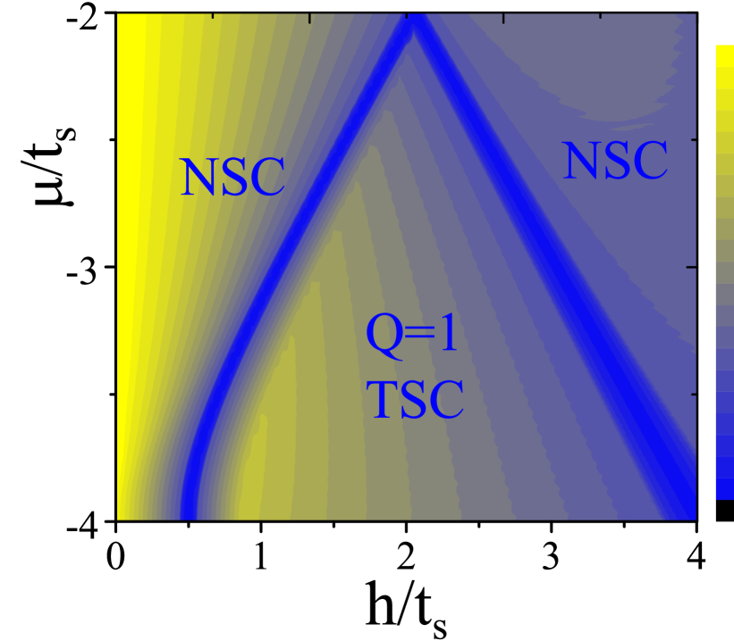
Figure 1: (Color online) The phase diagram ($\lambda=\Delta=0.5t_{s}$): The blue lines are the boundaries between the $\mathcal{Q}=1$ topological SC (TSC) and the normal SC (NSC) with trivial topological properties. The color denotes the size of the energy gap.

In Fig.1, we plot the global phase diagram. The blue lines are the boundaries between the topological SC and the SC with trivial topological properties. In the topological SC, the ground state has a nontrivial topological invariant (Chern-number) $\mathcal{Q}=1$MS . Such topological invariant is robust, for the Rashba SO coupling can be mapped into a $p+ip$ SC gap through a suitable unitary transformation (see details in Ref.MS ). We also study the density of state (DOS) in the topological superconductor numerically and show the results in Fig.2. From this result one can see that there exists a finite energy gap of the topological SC state. In other regions of the phase diagram, the ground states are the SC state with trivial topological properties.

Figure 2: (Color online) The density of states (DOS) of the $s$-wave SC model for the case of $u=-4t_{s}$, $\lambda=0.5t_{s}$, $\Delta=0.5t_{s}$, and $h=0.8t_{s}$. There exists an energy gap $\Delta E=0.7t_{s}$.

Figure 3: (Color online) The spectral flow of Hamiltonian $H$ on cylinder with $u=-4t_{s}$, $\lambda=0.5t_{s}$, $\Delta=0.5t_{s}$, and $h=0.8t_{s}$ for (a) but $h=0.4t_{s}$ for (b). For topological SC, there exist chiral gapless edge states in (a); while for normal SC there is no edge state in (b).

The operators of the Majorana edge states of this topological SC as shown in Fig.3 satisfy $\gamma_{0}^{{\dagger}}=\gamma_{0}$ , which indicates the edge states are really Majorana fermions. Indeed, we can see that the particle-hole operator $\mathcal{C}=\sigma^{x}\otimes\mathbf{1}$ acts on $\mathcal{H}(k)$ as

$$\mathcal{C}\mathcal{H}(k)\mathcal{C}^{-1}=-\mathcal{H}^{\ast}(-k)$$ (7)

implies that the Bogoliubov quasi-particle operator follows $\gamma_{-k}^{{\dagger}}=\gamma_{k}$ . From Fig.3 (a), one can find that the Majorana edge modes cross zero energy at $k_{y}=0$ for the topological SC with $u=-4t_{s}$, $\lambda=0.5t_{s}$, $h=0.8t_{s}$. The odd number of crossings leads to the topological protected Majorana zero modes. For the trivial SC with $u=-4t_{s}$, $\lambda=0.5t_{s}$, $h=0.4t_{s},$ there is no such crossing (Fig.3 (b)).

III Majorana zero modes around vortices of the topological SC

III.1 Majorana zero modes around a pair of vortices

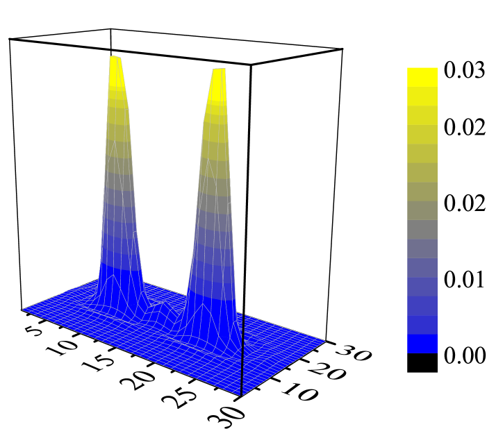
Figure 4: (Color online) The particle density distribution of two localized zero mode states around the two $\pi$-flux-vortices for the case of $u=-4t_{s},$ $\lambda=0.5t_{s},$ $h=0.8t_{s},$ $\Delta=0.5t_{s}.$

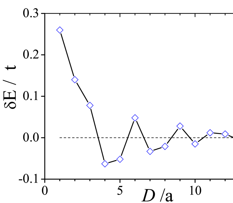
Figure 5: (Color online) The energy splitting $\delta E$ as the function of the spacial distance of two $\pi$-flux-vortices, decays exponentially and shows the oscillating behavior with $D$. The parameters are chosen as $u=-4t_{s},$ $\lambda=0.5t_{s},$ $h=0.8t_{s},$ $\Delta=0.5t_{s}$. $a$ is the lattice constant.

We now start with the discussion on the Majorana zero modes which associate with a pair of $\pi$-flux-vortices. The particle density distribution of the electrons is shown in Fig.4. The main result shows that there appear two approximately zero modes in the presence of two well-separated $\pi$-flux-vortices. When two $\pi$-fluxes are well separated, the quantum tunneling effect can be ignored and we have two quantum states with zero energy. On the other hand, for the small spatial distance $D$, the vortices interaction becomes stronger and the energy splitting can not be neglected. As shown in Fig.5, the energy splitting $\delta E$ as the function of $D$, oscillates and decreases exponentially. Likewise, a pair of $\pi$-flux-vortices in the topological $p$-wave SC or quasi-hole in the Moore-Read state has the qualitative similar behaviorMCH ; MCH2 ; MBA .

III.2 Topological properties of the topological SC with a square vortex-lattice

Next, we study the topological SC with a square vortex-lattice numerically. The illustration of the vortex-lattice ($\pi$-flux-lattice) was shown in Fig.6.

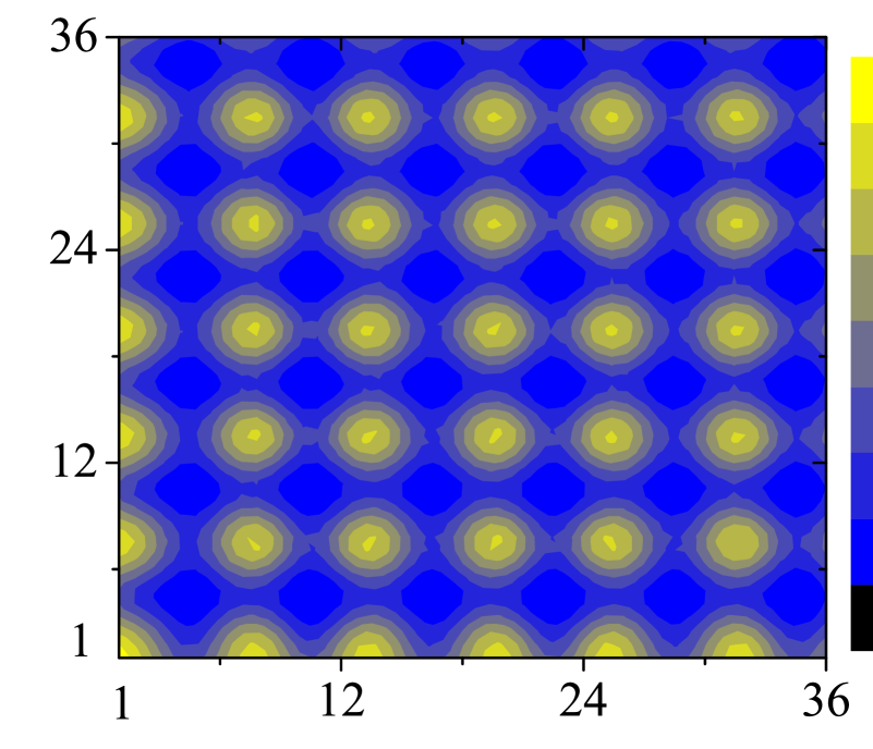
Figure 6: (Color online) The illustration of vortex-lattice: the distance between two nearest vortices is $6a$. The parameters are chosen as $u=-4t_{s},$ $\lambda=0.5t_{s},$ $h=0.8t_{s},$ $\Delta=0.5t_{s}$. Each vortex traps a Majorana mode. Thus, in Sec.IV we have a tight-binding Majorana lattice model to describe the low energy physics of the multi-Majorana-mode.

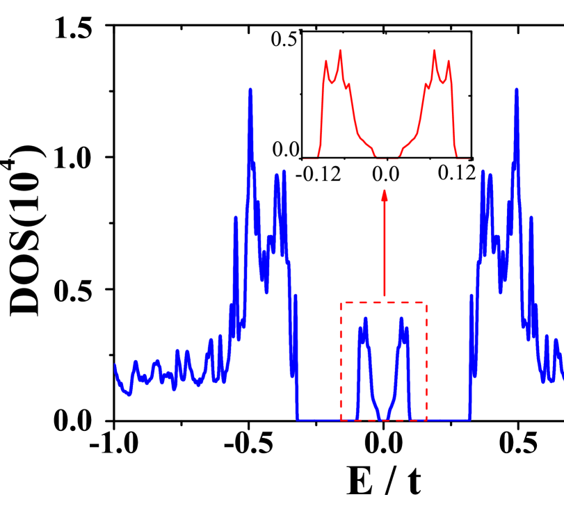
Figure 7: (Color online) The DOS of topological SC with square vortex-lattice: the mid-gap states are induced by the vortex-lattice. The inset shows the details of the mid-gap energy band.

The tunneling effect between vortices would lead to the coupling between two Majorana fermions around the vortices. Thus there exists a mid-gap energy band for the Majorana fermions. We study the density of state (DOS) in the topological SC with a square vortex-lattice numerically and the results are shown in Fig.7. From Fig.7, one can see that besides the energy bands of the paired electrons there exists a mid-gap energy band in parent topological SC. In particular, the mid-gap energy band has finite energy gap. It means that this mid-gap system as shown in Fig.7 may be a topological state associated with a non-trivial topological number intuitively. To check the topological properties of the mid-gap system, we calculate its edge states. We consider a system on a cylinder with $12$ super-unitcells along $x$-direction while periodic boundary along $y$-direction. Thus, $k_{y}$ is still a good quantum number and permits the Fourier transformation $c_{k_{y}}(j_{x})=\frac{1}{\sqrt{L_{y}}}\sum_{j_{y}}c(j_{x},j_{y})e^{ik_{y}j_{y}}.$ The spectral flow of this system on a cylinder is plotted in Fig.8. From Fig.8, one can see that two gapless chiral edge states are localized at the boundaries. On the other hand, we also plot the spectral flow in Fig.9. When the parent SC is a non-topological SC, the edge states disappear. As a result, we conclude that the mid-gap system shown in Fig.7 is indeed a topological state. From Fig.9, we also observe the disappear of the mid-gap band which is induced by the vortex-lattice. So the Majorana mode around the $\pi$-flux is protected by topological invariant of the parent $s$-wave SC.

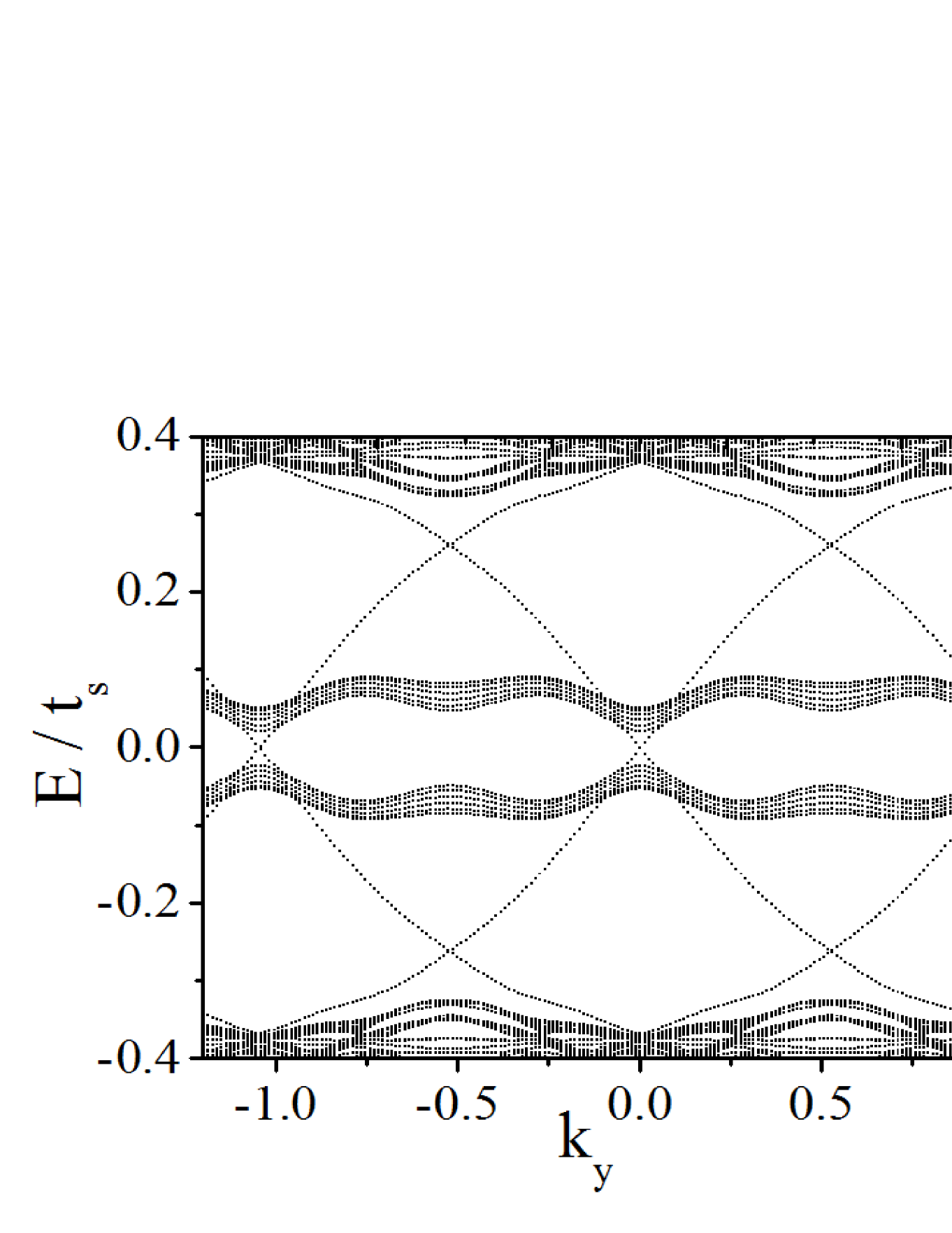
Figure 8: (Color online) The spectrum flow of topological SC with square vortices lattice on a cylinder. There exist gapless edge states for the case of $u=-4t_{s}$, $h=0.8t_{s}$, $\lambda=0.5t_{s}$, $\Delta=0.5t_{s}$.

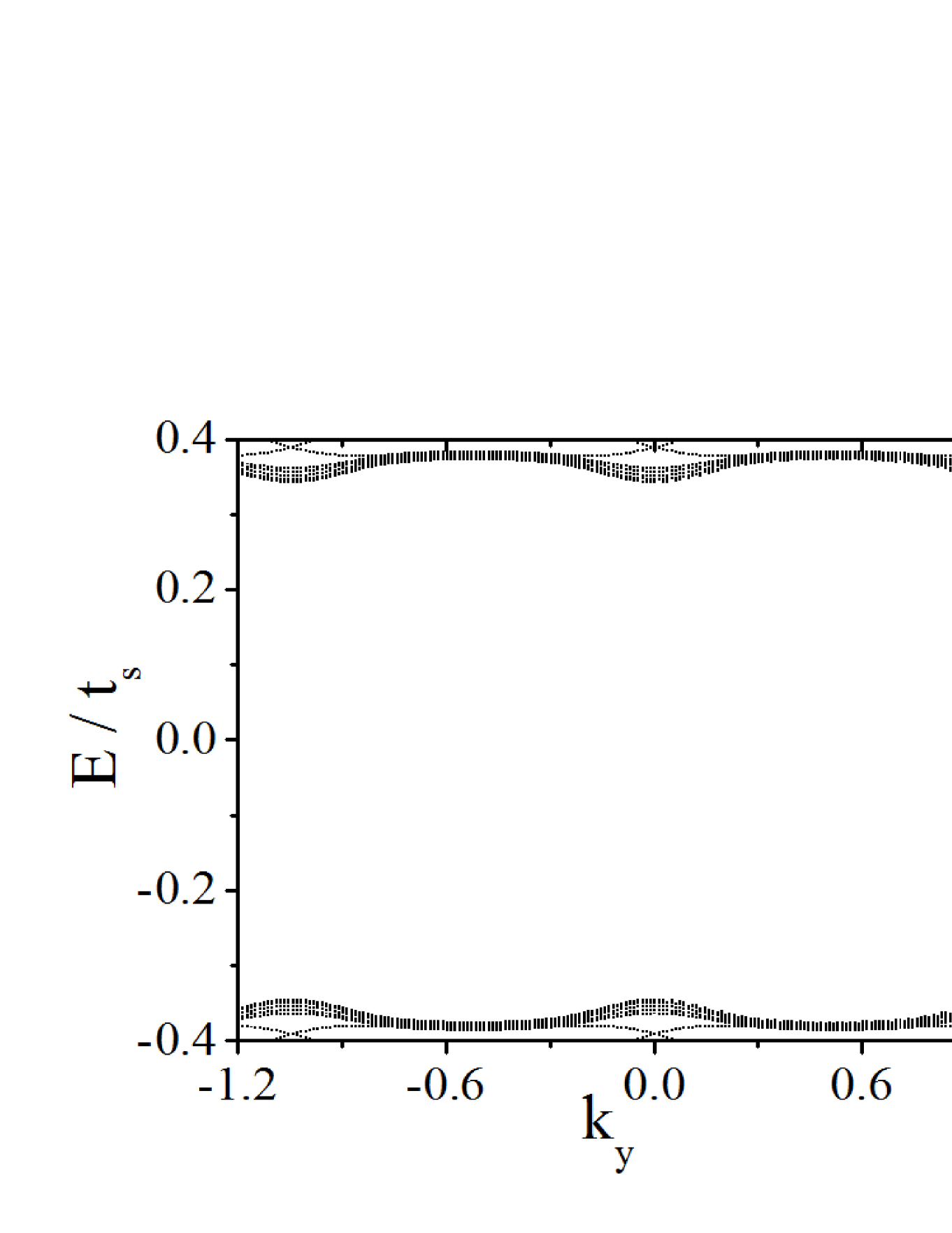
Figure 9: (Color online) The spectrum flow of normal SC with square vortex-lattice on a cylinder. The parameters are $u=-4t_{s}$, $h=0.2t_{s}$, $\lambda=0.5t_{s}$, $\Delta=0.5t_{s}$. There is no edge state.

IV The topological Majorana lattice model

In the last section we found a topological mid-gap system of the s-wave topological SC with a square vortex-lattice numerically. In this section we will learn the nature of this topological mid-gap system analytically.

We propose an effective description of the $s$-wave topological SC with a square vortex-lattice, of which each vortex traps a Majorana zero mode and two Majorana zero modes couple with each other by a short range interaction. The interaction strength is just the energy splitting $\delta E$ from the intervortex quantum tunneling. We call this effective description as the Majorana lattice model, of which the tight-binding Hamiltonian can be written as

$$\mathcal{H}_{m.f}=i\sum_{(j,k)}s_{jk}t_{jk}\gamma_{k}\gamma_{j}$$ (8)

where $t_{jk}$ is the hopping amplitude from $j$ to $k$, and satisfies $t_{jk}=t_{jk}^{\ast}$. $\gamma_{j}$ is a Majorana operator ($\gamma_{j}^{{\dagger}}=\gamma_{j}$) obeying anti-commutate relation $\{\gamma_{j},\gamma_{k}\}=2\delta_{jk}$. $s_{ij}=-s_{ji}$ is a gauge factor. The pair $(j,k)$ denotes the summation that runs over all the nearest neighbor (NN) pairs (with hopping amplitude $t$) and all the next-nearest neighbor (NNN) pairs (with hopping amplitude $t^{\prime}$). From the polygon rule proposed in Ref.EGR , each triangular plaquette possesses $\pi/2$ quantum flux effectively. This Hamiltonian allows a $Z_{2}$ gauge choice $s_{jk}=\pm 1$. For our Majorana lattice model, one possible gauge is given by Fig.10. Thus, the total number of Majorana modes $N$ must be even and then we can divide the Majorana lattice into two sublattices.

Then the Majorana modes can be combined pairwise to create $N/2$ complex fermionic states by pairing the Majorana operators as

$$\gamma_{2j-1}^{a}=a_{j}+a_{j}^{{\dagger}},\quad\gamma_{2j}^{b}=(a_{j}-a_{j}^{{\dagger}})/i$$ (9)

where $a_{j}$ ($a_{j}^{{\dagger}}$) annihilates (creates) a fermion at link $j$. In terms of operator $a_{j}$, the Majorana Hamiltonian takes the form of a ”topological SC” state as follows:

$$\mathcal{H}_{m.f} =\sum_{\mathbf{x}}\big{[}t(a_{\mathbf{x}}^{{\dagger}}a_{\mathbf{x}+\mathbf{j}}-a_{\mathbf{x}}a_{\mathbf{x}+\mathbf{j}}^{{\dagger}})+t(a_{\mathbf{x}}a_{\mathbf{x}+\mathbf{j}}-a_{\mathbf{x}}^{{\dagger}}a_{\mathbf{x}+\mathbf{j}}^{{\dagger}})$$

$$+2t(a_{\mathbf{x}}^{{\dagger}}a_{\mathbf{x}+\mathbf{i}}-a_{\mathbf{x}}a_{\mathbf{x}+\mathbf{i}}^{{\dagger}})-2it(a_{\mathbf{x}}a_{\mathbf{x}+\mathbf{i}}+a_{\mathbf{x}}^{{\dagger}}a_{\mathbf{x}+\mathbf{i}}^{{\dagger}})$$

$$+t^{\prime}(a_{\mathbf{x}}^{{\dagger}}a_{\mathbf{x}+\mathbf{i}-\mathbf{j}}-a_{\mathbf{x}}a_{\mathbf{x}+\mathbf{i}-\mathbf{j}}^{{\dagger}}-a_{\mathbf{x}}a_{\mathbf{x}+\mathbf{i}-\mathbf{j}}+a_{\mathbf{x}}^{{\dagger}}a_{\mathbf{x}+\mathbf{i}-\mathbf{j}}^{{\dagger}})$$

$$+t^{\prime}(a_{\mathbf{x}}^{{\dagger}}a_{\mathbf{x}+\mathbf{i}+\mathbf{j}}-a_{\mathbf{x}}a_{\mathbf{x}+\mathbf{i}+\mathbf{j}}^{{\dagger}}+a_{\mathbf{x}}a_{\mathbf{x}+\mathbf{i}+\mathbf{j}}-a_{\mathbf{x}}^{{\dagger}}a_{\mathbf{x}+\mathbf{i}+\mathbf{j}}^{{\dagger}})$$

$$-t(a_{\mathbf{x}}^{{\dagger}}a_{\mathbf{x}}-a_{\mathbf{x}}a_{\mathbf{x}}^{{\dagger}})\big{]}$$ (10)

where $\mathbf{i}$ and $\mathbf{j}$ are two orthogonal unit vectors (Fig.10).

Figure 10: Two sublattices of the Majorana lattice: $\gamma^{a}$ and $\gamma^{b}$. The arrows denote the $e^{i\pi/2}$ of the hopping parameters. Accordingly, there exists $\pi/2$ in each triangular plaquette. The lattice constant of the Majorana lattice model is $b=6a$.

Performing a Fourier transformation $a_{k}=\frac{1}{\sqrt{L_{\mathbf{x}}}}\sum_{\mathbf{x}}a_{\mathbf{x}}e^{-ikR_{\mathbf{x}}},$ the Hamiltonian becomes

$$\mathcal{H}_{m.f}=\sum_{k,a}\psi_{k}^{{\dagger}}d^{a}(k)\tau_{a}\psi_{k}$$ (11)

in the basis $\psi_{k}^{{\dagger}}=(a_{k}^{{\dagger}},a_{-k})$, where $a=x,y,z$, $\tau_{a}$ is the Pauli matrix, and

$$\begin{split}d^{z}(k)&=-2t\sin^{2}k_{y}+4t^{\prime}\cos k_{x}\cos^{2}k_{y}\\ d^{y}(k)&=-\sin 2k_{y}(t+2t^{\prime}\cos k_{x})\\ d^{x}(k)&=-2t\sin k_{x}\end{split}$$ (12)

See the detailed calculations in Appendix. Then we get the energy spectrum $E(k)$ of the Majorana lattice model as

$$E(k)=\pm\sqrt{\sum_{a=x,y,z}\left|d_{a}(k)\right|^{2}}.$$ (13)

From this result we can derive that there always exists an energy gap of the Majorana lattice model as long as $t^{\prime}\neq 0$. Then we calculate the DOS of the Majorana lattice model and show the result in Fig.11. One may compare the DOS of the Majorana lattice model in Fig.11 and the DOS of the mid-gap system in Fig.7 and find the similarity between them.

Figure 11: (Color online) The DOS of Majorana lattice model for the case of $t=0.048t_{s}$ and $t^{\prime}=0.006t_{s}$.

To characterize the topological properties of the Majorana lattice model, we define the nontrivial topological invariant - the Chern number

$$\mathcal{Q}=\frac{1}{4\pi}\int\int_{BZ}d^{2}k\frac{1}{|\mathbf{d}(k)|^{3}}\mathbf{d}(k)\cdot\frac{\partial\mathbf{d}(k)}{\partial k_{x}}\times\frac{\partial\mathbf{d}(k)}{\partial k_{y}}$$ (14)

which measures that the unit vector $\mathbf{d}(k)/|\mathbf{d}(k)|$ maps the Brillouin zone boundary onto sphere $S^{2}$ via the Chern number $\mathcal{Q}$. In the presence of NNN hopping $t^{\prime}$, we have $\mathcal{Q}=\pm 1$. Furthermore, we calculate the edge states of the Majorana lattice model and present the result in Fig.12. One may compare the spectrum of the edge states of the Majorana lattice model in Fig.12 with that of the mid-gap system in Fig.8 and also find the similarity between them. Now we can conclude that the (topological) Majorana lattice model captures the key low energy physics of the topological SC with a square vortex-lattice.

Figure 12: (Color online) The edge state of Majorana lattice model for the case of $t=0.048t_{s}$, $t^{\prime}=0.006t_{s}.$

In addition, we finish this section by a brief discussion of the $s$-wave topological SC with triangle vortex-lattice. If in the region of $|t^{\prime}/t|<<1$, we observe that the model is characterized by the winding number $\mathcal{Q}=\pm 1$, and this may stem from the redundant NN hopping (which behave as the NNN hopping of the square Majorana lattice model) of the triangular lattice. Moreover, the exotic phase $\mathcal{Q}=\pm 3$ can be reached by varying of the ratio $t^{\prime}/t$. In the region of $|t^{\prime}/t|>>1$, the triangular Majorana lattice model has a $\mathcal{Q}=\pm 3$ phase. It’s worth to point out that, for the triangular Majorana lattice model in $p+ip$ SC, or interacting vortex-lattice in Kitaev’s honeycomb model, people may find similar phase diagramVILL ; p .

V Conclusion

In the end, we draw a conclusion. In this paper we studied the properties of an $s$-wave topological SC with a square vortex-lattice. Because each vortex traps a Majorana zero mode, when we took into account of zero mode tunneling that couples the vortex sites, the Majorana zero modes of the vortex-lattice form a Majorana lattice model. We found that this Majorana lattice model shows nontrivial topological properties, including a nonvanishing Chern number, chiral Majorana edge state. In this sense, the Majorana lattice model is really a ”topological SC” on the parent topological SC. And the ”topological SC” induced by the vortex lattice is topologically protected by the topological invariant of the parent $s$-wave SC. Such correspondence between the topological properties of the Majorana lattice model and the topological properties of the $s$-wave topological SC model with vortex-lattice is another holographic feature of the topological state. In addition, we also had used the numerical approach to study the $s$-wave topological SC with a square vortex-lattice and got similar results.

Furthermore, the Majorana lattice model for chiral $p+ip$ topological superconductor with vortex-lattice and that for the coupled system due to the proximity effect between $s$-wave SC and three dimensional topological insulator with vortex-lattice have the same topological properties to our case. Thus, this approach paves a new way to observe the Majorana modes for the topological SC.

Appendix A Fourier transformation of the Hamiltonian for the Majorana lattice model

The Hamiltonian of the Majorana lattice model can be obtained by Fourier transformation $a_{\mathbf{x}}=1/\sqrt{L_{\mathbf{x}}}\sum_{\mathbf{k}}a_{\mathbf{k}}e^{-i\mathbf{k}R_{\mathbf{x}}},$

$$\mathcal{H}_{m.f} =1/L_{\mathbf{x}}\sum_{\mathbf{k},\mathbf{k^{\prime}}}\sum_{\mathbf{x}}$$

$$\{t(a_{\mathbf{k}}^{{\dagger}}a_{\mathbf{k^{\prime}}}e^{i\mathbf{k}R_{\mathbf{x}}-i\mathbf{k^{\prime}}R_{\mathbf{x}+\mathbf{j}}}-a_{\mathbf{k}}a_{\mathbf{k^{\prime}}}^{{\dagger}}e^{-i\mathbf{k}R_{\mathbf{x}}+i\mathbf{k^{\prime}}R_{\mathbf{x}+\mathbf{j}}})$$

$$+t(a_{\mathbf{k}}a_{\mathbf{k^{\prime}}}e^{-i\mathbf{k}R_{\mathbf{x}}-i\mathbf{k^{\prime}}R_{\mathbf{x}+\mathbf{j}}}-a_{\mathbf{k}}^{{\dagger}}a_{\mathbf{k^{\prime}}}^{{\dagger}}e^{i\mathbf{k}R_{\mathbf{x}}+i\mathbf{k^{\prime}}R_{\mathbf{x}+\mathbf{j}}})$$

$$+2t^{\prime}(a_{\mathbf{k}}^{{\dagger}}a_{\mathbf{k^{\prime}}}e^{i\mathbf{k}R_{\mathbf{x}}-i\mathbf{k^{\prime}}R_{\mathbf{x}+\mathbf{i}}}-a_{\mathbf{k}}a_{\mathbf{k^{\prime}}}^{{\dagger}}e^{-i\mathbf{k}R_{\mathbf{x}}+i\mathbf{k^{\prime}}R_{\mathbf{x}+\mathbf{i}}})$$

$$-2it(a_{\mathbf{k}}a_{\mathbf{k^{\prime}}}e^{-i\mathbf{k}R_{\mathbf{x}}-i\mathbf{k^{\prime}}R_{\mathbf{x}+\mathbf{i}}}+a_{\mathbf{k}}^{{\dagger}}a_{\mathbf{k^{\prime}}}^{{\dagger}}e^{i\mathbf{k}R_{\mathbf{x}}+i\mathbf{k^{\prime}}R_{\mathbf{x}+\mathbf{i}}})$$

$$+t^{\prime}(a_{\mathbf{k}}^{{\dagger}}a_{\mathbf{k^{\prime}}}e^{i\mathbf{k}R_{\mathbf{x}}-i\mathbf{k^{\prime}}R_{\mathbf{x}+\mathbf{i}-\mathbf{j}}}-a_{\mathbf{k}}a_{\mathbf{k^{\prime}}}^{{\dagger}}e^{-i\mathbf{k}R_{\mathbf{x}}+i\mathbf{k^{\prime}}R_{\mathbf{x}+\mathbf{i}-\mathbf{j}}})$$

$$-t^{\prime}(a_{\mathbf{k}}a_{\mathbf{k^{\prime}}}e^{-i\mathbf{k}R_{\mathbf{x}}-i\mathbf{k^{\prime}}R_{\mathbf{x}+\mathbf{i}-\mathbf{j}}}-a_{\mathbf{k}}^{{\dagger}}a_{\mathbf{k^{\prime}}}^{{\dagger}}e^{i\mathbf{k}R_{\mathbf{x}}+i\mathbf{k^{\prime}}R_{\mathbf{x}+\mathbf{i}-\mathbf{j}}})$$

$$+t^{\prime}(a_{\mathbf{k}}^{{\dagger}}a_{\mathbf{k^{\prime}}}e^{i\mathbf{k}R_{\mathbf{x}}-i\mathbf{k^{\prime}}R_{\mathbf{x}+\mathbf{i}+\mathbf{j}}}-a_{\mathbf{k}}a_{\mathbf{k^{\prime}}}^{{\dagger}}e^{-i\mathbf{k}R_{\mathbf{x}}+i\mathbf{k^{\prime}}R_{\mathbf{x}+\mathbf{i}+\mathbf{j}}})$$

$$+t^{\prime}(a_{\mathbf{k}}a_{\mathbf{k^{\prime}}}e^{-i\mathbf{k}R_{\mathbf{x}}-i\mathbf{k^{\prime}}R_{\mathbf{x}+\mathbf{i}+\mathbf{j}}}-a_{\mathbf{k}}^{{\dagger}}a_{\mathbf{k^{\prime}}}^{{\dagger}}e^{i\mathbf{k}R_{\mathbf{x}}+i\mathbf{k^{\prime}}R_{\mathbf{x}+\mathbf{i}+\mathbf{j}}})$$

$$-t(a_{\mathbf{k}}^{{\dagger}}a_{\mathbf{k^{\prime}}}e^{i\mathbf{k}R_{\mathbf{x}}-i\mathbf{k^{\prime}}R_{\mathbf{x}}}-a_{\mathbf{k}}a_{\mathbf{k^{\prime}}}^{{\dagger}}e^{-i\mathbf{k}R_{\mathbf{x}}+i\mathbf{k^{\prime}}R_{\mathbf{x}}})\}$$ (15)

where $R_{\mathbf{x}+\mathbf{\delta}}=R_{\mathbf{x}}+\mathbf{\delta}$, ($\mathbf{\delta}=\mathbf{i},\mathbf{j},\mathbf{i}+\mathbf{j}$). Using the identity $\delta_{\mathbf{k},\mathbf{k}^{\prime}}=1/L_{\mathbf{x}}\sum_{\mathbf{x}}e^{i(\mathbf{k}-\mathbf{k}^{\prime})R_{\mathbf{x}}}$, we have

$$\mathcal{H}_{m.f} =\sum_{\mathbf{k}}\{t(a_{k}^{{\dagger}}a_{k}e^{-ik_{y}}-a_{k}a_{k}^{{\dagger}}e^{ik_{y}})$$

$$+t(a_{k}a_{-k}e^{ik_{y}}-a_{k}^{{\dagger}}a_{-k}^{{\dagger}}e^{-ik_{y}})$$

$$+2t^{\prime}(a_{k}^{{\dagger}}a_{k}e^{-ik_{x}}-a_{k}a_{k}^{{\dagger}}e^{ik_{x}})$$

$$-2it(a_{k}a_{-k}e^{ik_{x}}+a_{k}^{{\dagger}}a_{-k}^{{\dagger}}e^{-ik_{x}})$$

$$+t^{\prime}(a_{k}^{{\dagger}}a_{k}e^{-i(k_{x}-k_{y})}-a_{k}a_{k}^{{\dagger}}e^{i(k_{x}-k_{y})})$$

$$-t^{\prime}(a_{k}a_{-k}e^{i(k_{x}-k_{y})}-a_{k}^{{\dagger}}a_{-k}^{{\dagger}}e^{-i(k_{x}-k_{y})})$$

$$+t^{\prime}(a_{k}^{{\dagger}}a_{k}e^{-i(k_{x}+k_{y})}-a_{k}a_{k}^{{\dagger}}e^{i(k_{x}+k_{y})})$$

$$+t^{\prime}(a_{k}a_{-k}e^{i(k_{x}+k_{y})}-a_{k}^{{\dagger}}a_{-k}^{{\dagger}}e^{-i(k_{x}+k_{y})})$$

$$-t(a_{k}^{{\dagger}}a_{k}-a_{k}a_{k}^{{\dagger}})\}$$ (16)

which is

$$\mathcal{H}_{m.f} =(t\cos k_{y}+2t^{\prime}\cos k_{x}+2t^{\prime}\cos k_{x}\cos k_{y})a_{k}^{{\dagger}}a_{k}$$

$$-(t\cos k_{y}+2t^{\prime}\cos k_{x}+2t^{\prime}\cos k_{x}\cos k_{y})a_{k}a_{k}^{{\dagger}}$$

$$-(2t\sin k_{x}+it\sin k_{y}+2it^{\prime}\sin k_{y}\cos k_{x})a_{-k}a_{k}$$

$$-(2t\sin k_{x}-it\sin k_{y}-2it^{\prime}\sin k_{y}\cos k_{x})a_{k}^{{\dagger}}a_{-k}^{{\dagger}}$$ (17)

or

$$\mathcal{H}_{m.f}=\sum_{\mathbf{k}}\sum_{a=x,y,z}\psi_{\mathbf{k}}^{{\dagger}}d^{a}(\mathbf{k})\sigma_{a}\psi_{\mathbf{k}}.$$ (18)

where $\psi_{\mathbf{k}}^{{\dagger}}=(a_{\mathbf{k}}^{{\dagger}},a_{-\mathbf{k}}).$

References

• (1) Y. Tsutsumi, T. Kawakami, T. Mizushima, M. Ichioka, and K. Machida, Phys. Rev. Lett. 101, 135302 (2008).
• (2) S. Das Sarma, C. Nayak, and S. Tewari, Phys. Rev. B 73, 220502R (2006).
• (3) L. Fu and C. L. Kane, Phys. Rev. Lett. 100, 096407 (2008).
• (4) N. Read and D. Green, Phys. Rev. B 61, 10267 (2000).
• (5) M. Sato, Y. Takahashi, and S. Fujimoto, Phys. Rev. Lett. 103, 020401 (2009).
• (6) J. D. Sau, R. M. Lutchyn, S. Tewari, and S. Das Sarma, Phys. Rev. Lett. 104, 040502 (2010).
• (7) R. M. Lutchyn, J. D. Sau, and S. Das Darma, Phys. Rev. Lett. 105, 077001 (2010).
• (8) D. A. Ivlovik, Phys. Rev. Lett. 86, 268 (2001).
• (9) I. P. Radu, J. B. Miller, C. M. Marcus, M.A.Kastner, L. N. Pfeiffer, K. W. West, Science 320, 899 (2008).
• (10) W. Bishara, P. Bonderson, C. Nayak, K. Shtengel, J. K. Slingerland, Phys. Rev. B 80, 155303 (2009).
• (11) J. Alicea, Phys. Rev. B 81, 125318 (2010).
• (12) C. Nayak, S. H. Simon, A. Stern, M. Freedman, and S. Das Sarma, Rev. Mod. Phys. 80, 1083 (2008).
• (13) S. Das Sarma, M. Freedman, and C. Nayak. Phys. Rev. Lett. 94, 166802 (2005).
• (14) S. Tewari, S. Das Sarma, C. Nayak, C. Zhang, and P. Zoller, Phys. Rev. Lett. 98, 010506 (2007).
• (15) A. Kitaev, Ann. Phys. 303, 2 (2003). A. Kitaev, Ann. Phys. 321, 2 (2006).
• (16) C. Gils, E.Ardonne, S. Trebst, A. W. W. Ludwig, M. Troyer, and Z. Wang, Phys. Rev. Lett. 103, 070401 (2009).
• (17) A. Feiguin, S. Trebst, A. W. W. Ludwig, M. Troyer, A. Kitaev, Z. Wang, and M. H. Freedman, Phys. Rev. Lett. 98, 160409 (2007).
• (18) M. Cheng, R. M. Lutchyn, V. Galitski, and S. Das Sarma, Phys. Rev. B 82, 094504 (2010).
• (19) M. Cheng, R. M. Lutchyn, V. Galitski, and S. Das Sarma, Phys. Rev. Lett 103, 107001 (2009).
• (20) A. Stern, F. von Oppen, and E. Mariani, Phys. Rev. B 70, 205338 (2004).
• (21) V. Gurarie, and L. Radzihovsky, Ann. Phys. 322, 2 (2007).
• (22) T. Mizushima, M. Ichioka, and K. Machida, Phys. Rev. Lett. 101, 150409 (2008).
• (23) C. Zhang, S. Tewari, R. M. Lutchyn, and S. Das Sarma, Phys. Rev. Lett. 101, 160401 (2008).
• (24) N. R. Cooper, and G. V. Shiyapnikov, Phys. Rev. Lett. 103,155302 (2009).
• (25) Y. Nishida, Ann. Phys. (N.Y.) 324, 897 (2009).
• (26) V. Lahtinen, A. W. Ludwig, J. K.Pachos, and S. Trebst, ArXiv:1111.3296.
• (27) M. Baraban, G. Zikos, N. Bonesteel, and S. H. Simon, ArXiv:0901.3502.
• (28) E. Grosfeld and Ady Stern, Phys. Rev. B 73, 201303 (2006).
• (29) J. K. Pachos, E. Alba, V. Lahtinen, J. J. Garcia-Ripoll, ArXiv:1209.5115.