Optimal Transmission Policy for Cooperative Transmission with Energy Harvesting and Battery Operated Sensor Nodes

Abstract

In this paper, we consider a scenario where one energy harvesting and one battery operated sensor cooperatively transmit a common message to a distant base station. The goal is to find the jointly optimal transmission (power allocation) policy which maximizes the total throughput for a given deadline. First, we address the case in which the storage capacity of the energy harvesting sensor is infinite. In this context, we identify the necessary conditions for such optimal transmission policy. On their basis, we first show that the problem is convex. Then we go one step beyond and prove that (i) the optimal power allocation for the energy harvesting sensor can be computed independently; and (ii) it unequivocally determines (and allows to compute) that of the battery operated one. Finally, we generalize the analysis for the case of finite storage capacity. Performance is assessed by means of computer simulations. Particular attention is paid to the impact of finite storage capacity and long-term battery degradation on the achievable throughput.

1 Introduction

Sensor nodes are typically powered by batteries that, quite often, are either costly, difficult or simply impossible to replace. Clearly, this limits network lifetime. Energy harvesting makes it possible to overcome this drawback by allowing sensors to harvest energy from e.g. solar, mechanical, or thermal sources. The harvested energy is typically stored in a device (e.g. battery, super capacitor) and then supplied for communication and/or processing tasks when needed. In recent years, many authors have analyzed how to optimally use such harvested energy. For single-sensor scenarios, in [1] the authors derive the optimal transmission policy which minimizes the time needed to deliver all data packets to the destination subject to causality constraints on energy and packet arrivals. In [2], the authors go one step beyond and, unlike [1], they consider finite storage capacity effects. In both cases, the energy harvesting instants and amounts of energy harvested are assumed to be known a priori. Ozel et al generalize the analysis to Rayleigh-fading channels and for the case in which the information on the harvested energy and channel gains is either causally or non-causally known [3]. Other works in the literature have addressed scenarios with multiple energy harvesting terminals. This includes studies for the multiple-access [4], interference [5], relay [6] and broadcast [7, 8] channels.

Distributed beamforming techniques allow nodes in a Wireless Sensor Network (WSN) to act as a virtual antenna array in order to reach a distant Base Station (BS) or data sink. This, however, requires accurate frequency and phase synchronization over sensors. To that aim, one can resort to the iterative synchronization scheme with one-bit of feedback proposed in [9], or opportunistic sensor selection schemes [10].

In this paper, we consider a scenario where one energy harvesting (EH) and one battery operated (BO) sensor cooperate to transmit (beamform) a common message to a distant base station. This differs from the scenarios in [4, 5, 6], where both sensors/terminals had energy harvesting capabilities. Our goal is to find the jointly optimal power allocation strategy which maximizes the total throughput for a given deadline (e.g. the time by which batteries could be replaced). This problem is equivalent to the one addressed e.g. in [1, 3] but here we consider the more general case with multiple transmitters. Besides, and unlike the Multiple-Access Channel (MAC) scenarios in [4], sensors here attempt to convey a common message to the destination. We also go one step beyond the distributed beamforming approaches in [9, 10] where, implicitly, all sensors were assumed to be battery operated, and investigate the impact of energy harvesting constraints on performance. As in [4], we initially assume that the energy harvesting sensor is equipped with a re-chargeable battery of infinite storage capacity. In this context, we identify the necessary conditions for the jointly optimal transmission policy. This leads to a problem that we show to be convex. Furthermore, and as an extension to our previous work in [11], we prove that the optimal policy for the EH node can be computed independently from that of the BO one, and propose an algorithm to compute the latter from the former. Next, we generalize the analysis for a scenario in which, as in [2], the storage capacity of the EH sensor is finite. We also consider imperfections in the re-chargeable battery of the EH sensor. More specifically, we focus on the impact of long-term capacity degradation, as opposed to the (short-time) battery leakage effects addressed in [12]

2 Signal and Communication Model

Two sensors cooperate to transmit a common message $m(t)$ to a distant base station. The received signal thus reads

$$r(t)=m(t)\left(\sum_{i=1}^{2}w_{i}(t)e^{j\psi_{i}(t)}\right)+n(t)$$ (1)

where the common message is given by $m(t)=\sum_{l}x_{l}g(t-lT_{s})$, with $\{x_{l}\}$ standing for a sequence of zero-mean complex Gaussian symbols with unit variance ($T_{s}$ is the symbol period) and $g(t)$ denoting the impulse response of a bandlimited pulse (unit bandwidth); $w_{i}(t)=\sqrt{p_{i}(t)}e^{j\phi_{i}(t)}$ denotes the time-varying complex transmit weights in polar notation (to be designed); $e^{j\psi_{i}(t)}$ stands for the phase shift of the (Gaussian) sensor-to-base station channels; and $n(t)$ is zero-mean complex additive white Gaussian noise with unit variance (i.e. $n(t)\sim\mathcal{CN}(0,1))$. In the sequel, we assume that by properly designing $\phi_{i}(t)$ the channel phase and, where relevant, oscillator offsets can be ideally pre-compensated [9]. Frequency and time synchronization is assumed, as well. Hence, the sensor network behaves as a virtual antenna array capable of beamforming the message to the base station. Without loss of generality, we let the first sensor be the one with energy harvesting capabilities, and the second to be battery operated. Consequently, we hereinafter denote by $p^{H}\!(t)\triangleq p_{1}(t)$ and $p^{B}\!(t)\triangleq p_{2}(t)$ the transmit power at the energy harvesting and battery operated sensors, respectively. Bearing all this in mind, the instantaneous received power at the base station is given by $p_{BF}\!(t)=(\sqrt{p^{H}\!(t)}+\sqrt{p^{B}\!(t)})^{2}$. The total throughput for a given deadline $T$ then reads

$$G_{T}(p^{H}\!(t),p^{B}\!(t))=\int_{0}^{T}\log\left(1+p_{BF}(t)\right)dt.$$ (2)

Our goal is to find the jointly optimal transmission (power allocation) policies $p^{H}\!(t)$ and $p^{B}\!(t)$ such that $G_{T}$ is maximized subject to the causality constraints imposed by the energy harvesting process, namely,

$$e^{H}\!(t)\leq E^{H}\!(t) \triangleq \sum_{k:s_{k}<t}E_{k}^{1}$$ (3)

$$e^{B}\!(t)\leq E^{B}\!(t) \triangleq E_{0}^{2},$$ (4)

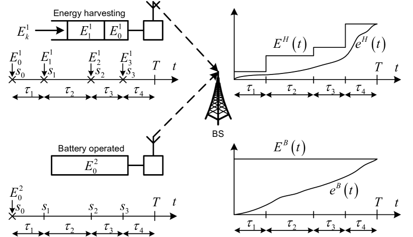
Figure 1: Network with energy harvesting and battery operated sensors (left); cumulative energy constraints and energy consumption curves (right).

for $0\leq t\leq T$, where $e^{H}\!(t)=\int_{0}^{t}p^{H}\!(\tau)d\tau$ and $e^{B}\!(t)=\int_{0}^{t}p^{B}\!(\tau)d\tau$ denote the energy consumption (EC) curves; and $E^{H}\!(t)$, $E^{B}\!(t)$ stand for the cumulative energy harvesting (cEH) constraints (see Fig. 1). In the above expression, $E_{k}^{i}$ accounts for the amount of energy harvested by sensor $i$ in the $k^{\text{th}}$ event ($k=0\ldots N-1$). We define event $s_{k}$ as the time instant in which some energy is harvested by any of the sensors in the network ($E_{k}^{i}=0$ for the sensor not harvesting any energy in that event). Both the events and the amounts of energy harvested $E_{k}^{i}$ are assumed to be known a priori. Further, we impose $E_{0}^{i}>0$ for all $i$ (sensors) so that collaborative transmission can start immediately, that is, from $t=0$. For battery operated sensors, we have $E_{k}^{i}=0$ for $k>0$ and, thus, the cumulative energy harvesting function is constant for the whole period. For the EH sensor, on the contrary, it is given by a staircase function. Finally, we define epoch as the time elapsed between two consecutive events $s_{k}$ and $s_{k-1}$. Its duration is given by $\tau_{k}\triangleq s_{k}-s_{k-1}$ for $k=1\ldots N-1$ and, likewise, we define $\tau_{N}\triangleq T-s_{N-1}$. A given transmission policy is said to be feasible (yet, perhaps, not optimal) if, as imposed by (3) and (4), the energy consumption curves lie below cumulative energy harvesting ones at all times (or occasionally hit them).

3 Necessary conditions for the optimality of the transmission policy

The following lemmas give the necessary optimality conditions under the assumption of infinite storage capacity for the EH sensor. Moreover, the insights gained into the problem structure allow us to compute the jointly optimal transmission policies in Section 4. Unless otherwise stated, the lemmas hold for both the energy harvesting and battery operated sensors.

Lemma 1.

The transmit power in each sensor remains constant between consecutive events.

In other words, the power/rate in each sensor only potentially changes when new energy arrives to any of them . The proof of this lemma, which is based on Jensen’s and Cauchy’s inequalities, can be found in Appendix A. This lemma implies that $p^{H}\!(t)=p^{H}_{k},p^{B}\!(t)=p^{B}_{k}$ for $s_{k-1}\leq t<s_{k}$. That is, the power allocation curves $p^{H}\!(t)$ and $p^{B}\!(t)$ are necessarily staircase functions and, hence, the energy consumption curves $e^{H}\!(t)$ and $e^{B}\!(t)$ are piecewise linear. This observation allows us to pose the original problem (2) in a convex optimization framework in which a numerical (or analytical) solution is easier to find. This will be accomplished in the next section.

Lemma 2.

All the harvested/stored energy must be consumed by the given deadline $T$.

This means that, necessarily, the cumulative energy harvesting curves reach the energy consumption constraints at time instant $T$.

Proof.

Lemma 2 can be easily proved by contradiction. Assume that the optimal transmission policy does not fulfill such condition. We could think of a feasible policy such that (i) the set of curves $e^{H}\!(t)$ and $e^{B}\!(t)$ differ from the optimal ones in the last epoch only, namely, for $t\in[s_{N-1}\ldots T)$; and (ii) it verifies $e^{H}\!(T)=E^{H}\!(T)$ and $e^{B}\!(T)=E^{B}\!(T)$. Being piecewise linear (and continuous), these curves would necessarily lie above the optimal ones at least in part of such last epoch, this resulting in a higher received power and throughput. This contradicts the optimality of the original transmission policy. ∎

Lemma 3.

If feasible, a transmission policy with constant transmit power in each sensor between any two (i.e. not necessarily consecutive) events turns out to be optimal for the period of time elapsed between these two events.

This lemma goes one step beyond and states that Lemma 1 also holds for non-consecutive events, as long as a constant transmit power policy in both sensors is feasible for this period. This follows directly from the proof of Lemma 1 but, since one or more energy harvests might take place in between the initial and final events, feasibility needs to be ensured (clearly, this is not needed in Lemma 1).

Lemma 4.

The transmit powers for an energy harvesting sensor with infinite storage capacity are monotonically increasing, i.e. $p^{H}_{1}\leq p^{H}_{2}\leq\ldots\leq p^{H}_{N}$

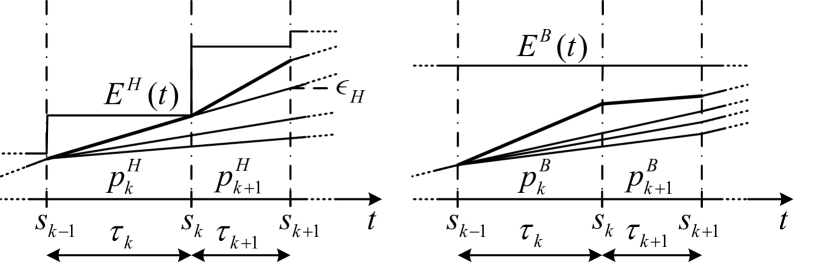
Figure 2: Transmit powers at the EH sensor are monotonically increasing (Lemma 4).

Proof.

This property follows from the fact that $E^{H}\!(t)$ is a staircase function. Assume that the power allocation policy before $s_{k-1}$ and after $s_{k+1}$ is optimal. As shown in Fig. 2, the optimal EC curve verifies $e^{H}\!(s_{k+1})\in\left(e^{H}\!(s_{k-1}),E^{H}\!(s_{k+1})\right]$. For $e^{H}\!(s_{k+1})\in\left(e^{H}\!(s_{k-1}),\epsilon_{H}\right]$, we know from Lemma 3 that a constant power allocation for the energy harvesting and battery operated sensors turns out to be optimal for $\left[s_{k-1},s_{k+1}\right)$ (and, hence, for $\left[0,T\right]$). In particular, this implies that $p^{H}_{k+1}=p^{H}_{k}$. For $e^{H}\!(s_{k+1})\in\left(\epsilon_{H},E^{H}\!(s_{k+1})\right]$, on the contrary, the fact that $e^{H}\!(t)$ is continuous and piecewise linear can only be ensured if (and only if) $p^{H}_{k+1}>p^{H}_{k}$. By repeatedly applying this reasoning to all consecutive epoch pairs the proof follows. As for the relationship between $p^{B}_{k+1}$ and $p^{B}_{k}$, nothing can be said yet. Still, the fact that $E^{B}\!(t)$ is a constant function does not impose any additional restrictions to the power allocation policy of the BO sensor in $\left[s_{k-1},s_{k+1}\right]$. ∎

Lemma 5.

Transmit powers are strictly positive.

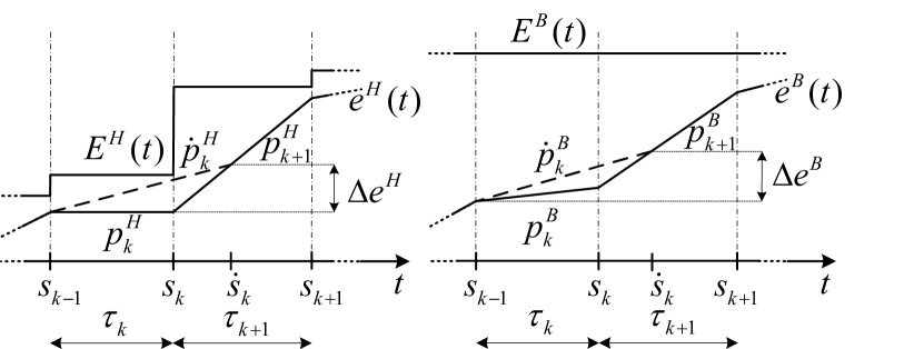
Figure 3: Transmit powers are strictly positive (Lemma 5)

Proof.

Again, this can be proved by contradiction. Assume that the power allocation policy before $s_{k-1}$ and after $s_{k+1}$ is optimal. Assume that, as shown in Fig. 3, the optimal policy for the $\left[s_{k-1},s_{k+1}\right)$ period verifies $p^{H}_{k}=0$ and $p^{H}_{k+1}>0$. One could think of a new (and feasible) transmission policy given by $\dot{p}^{H}_{k}=\frac{\Delta e^{H}}{\dot{s}_{k}-s_{k-1}}$ and $\dot{p}^{B}_{k}=\frac{\Delta e^{B}}{\dot{s}_{k}-s_{k-1}}$ for $t\in\left[s_{k-1},\dot{s}_{k}\right)$; and $\dot{p}^{H}_{k+1}=p^{H}_{k+1}$ along with $\dot{p}^{B}_{k+1}=p^{B}_{k+1}$ for $t\in\left[\dot{s}_{k},s_{k+1}\right)$. From the proof of Lemma 3, we know that the new policy achieves higher throughput than the original one in $\left[s_{k-1},\dot{s}_{k}\right)$ and, thus, in $\left[s_{k-1},s_{k+1}\right)$ too. Yet not optimal (since this new policy e.g. contradicts Lemma 1), this proves that the original policy given by $p^{H}_{k}=0$ and $p^{H}_{k+1}>0$ was not optimal either. Along the same lines, one can easily find a new feasible policy achieving higher throughput than $p^{B}_{k}=0$ and $p^{B}_{k+1}>0$ for the battery operated sensor. ∎

4 Computation of the optimal transmission policy

Lemma 1 allows us to re-write the original optimization problem given by the score function (2) and the causality constraints (3) and (4) as follows (to recall, our focus here is on scenarios where the storage capacity of the EH sensor is infinite):

$$\underset{\{p^{H}_{k}\}_{k=1}^{N},\{p^{B}_{k}\}_{k=1}^{N}}{\text{max}}\sum_{k=1}^{N}\tau_{k}\log\left(1+(\sqrt{p^{H}_{k}}+\sqrt{p^{B}_{k}})^{2}\right)$$ (5)

s.t.:

$$\quad\sum_{k=1}^{n}\tau_{k}p^{H}_{k}\leq E_{n}^{H}=\sum_{k=0}^{n-1}E_{k}^{1}\;\text{ for}\;n=1\ldots N$$ (6)

$$\quad\sum_{k=1}^{n}\tau_{k}p^{B}_{k}\leq E_{n}^{B}=E_{0}^{2}\;\text{ for}\;n=1\ldots N$$ (7)

$$\quad p^{H}_{k}>0\;\text{ for}\;k=1\ldots N$$ (8)

$$\quad p^{B}_{k}>0\;\text{ for}\;k=1\ldots N$$ (9)

where we have defined $E_{n}^{H}\triangleq E^{H}(t)$ for $t\in[s_{n-1},s_{n})$, and where the last two strict inequalities follow from Lemma 5. The problem is convex since all the constraints are affine and linear, and the objective function is concave, as we will prove next. To that aim, we observe that the $k^{\text{th}}$ term in the summation exclusively depends on the corresponding optimization variables $p^{H}_{k}$ and $p^{B}_{k}$ (i.e. no cross-term variables). Hence, it suffices to show that an arbitrary term in the summation, namely, $G_{1}(p^{H},p^{B})=\tau\log(1+(\sqrt{p^{H}}+\sqrt{p^{B}})^{2})$ is concave (indices have been omitted for brevity). Or, alternatively, that $G_{2}(p^{H},p^{B})=-G_{1}(p^{H},p^{B})$ is convex. The latter can be verified by realizing that, for $p^{H}>0$ and $p^{B}>0$, its $2\times 2$ Hessian is positive definite, namely, $\nabla^{2}G_{2}(p^{H},p^{B})\succ 0$. Since the optimization problem is strictly convex, its unique solution can at least be found numerically (e.g. by resorting to interior point methods). However, this task is computationally intensive, in particular when the number of energy harvesting events $N$ is large. This motivates the following lemma and two theorems from which a semi-analytical and less computationally intensive solution to the optimization problem can be obtained.

Lemma 6.

The jointly optimal power allocation policy is such that, whenever the transmit power changes, the energy consumed by the energy harvesting sensor up to that time instant, equals the energy harvested by such sensor up to that instant (i.e, the stored energy is zero).

The proof of this Lemma is based on the Karush-Kuhn-Tucker (K.K.T.) conditions associated to the (joint) optimization problem (5)-(9). Details can be found in Appendix B.

The next theorems state the main result of this paper since they allow to effectively compute the optimal transmissions policies for the EH and BO sensors, respectively.

Theorem 1.

The optimal transmission policy for the energy harvesting sensor, $\{\breve{p}^{H}_{k}\}_{k=1}^{N}$, can be computed independently from that of the battery operated one. The associated energy consumption curve turns out to be the shortest string starting in $t=0$, ending in $t=T$, and lying below the cumulative energy harvesting curve.

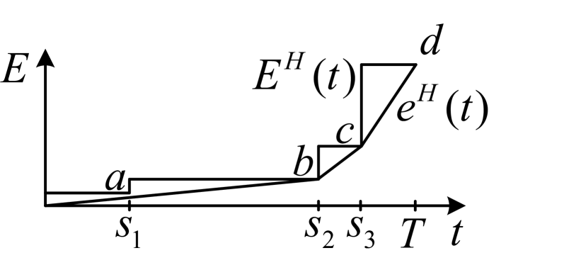
Figure 4: The optimal energy consumption curve for the EH sensor is given by the shortest string below the cumulative EH curve (Theorem 1)

Proof.

As we will prove next, Lemmas 1 to 6 unequivocally determine the optimal transmission policy for the EH sensor. First note that, in order to satisfy the energy causality constraint, the corresponding EC curve must lie below the cEH curve. From Lemma 2, it follows that the EC curve reaches the cEH curve at $t=T$. Besides, from Lemmas 1 and 3, we know that the transmit power only potentially changes at the energy harvesting events. Consequently, the optimal EC curve must be linear between them (i.e. piecewise linear). Moreover, Lemma 6 dictates that, whenever the transmit power (slope) changes at an energy harvesting event, the EC curve hits the cEH curve. Based on these facts, we conclude that the first linear part of EC curve must connect the origin with some corner point on the cEH curve (see Fig 4). Because of Lemma 4, we must choose the one with the minimal slope, since otherwise the constraint on energy causality (point $c$) or monotonicity property of Lemma 4 (point $a$) would not be satisfied. Clearly, in Fig 4 this corresponds to point $b$. Once this point is identified, the algorithm can be iteratively applied until we find the optimal policy until deadline $T$. As a result, the EC curve is given by the shortest string below the cEH curve. It must be noted that this algorithm is equivalent to the one presented in [1]. However, the interesting points are that (i) we have proved that it continues to be optimal in a scenario where two sensors, one of them battery operated, collaborate to send the message (vs. one sensor in [1]); and that (ii) no information on the BO sensor (i.e. its optimal EC curve) is needed to determine it. ∎

Theorem 2.

Upon finding the optimal transmission policy for the energy harvesting sensor, the optimal transmission policy for the battery operated one, $\{\breve{p}^{B}_{k}\}_{k=1}^{N}$, can be computed with the iterative procedure given by Algorithm 1.

Algorithm 1 Optimal policy for the battery operated sensor

1:choose some small $\delta>0$ $\triangleright$ Step for searching

2:$m:=0$ $\triangleright$ Iteration index

3:$E^{B}_{T}:=E_{0}^{2}$ $\triangleright$ Energy stored in the battery

4:repeat

5:     $m:=m+1$

6:     for all $k=1\ldots N$ do

7:         $B_{k,m}:=m\delta$,

8:         solve $\breve{p}^{H}_{k}=\frac{B_{k,m}(A_{k,m}+B_{k,m}-A_{k,m}B_{k,m})}{A_{k,m}(A_{k,m}+B_{k,m})^{2}}$ for $A_{k,m}$

9:         $p^{B}_{k,m}\leftarrow\left(\frac{A_{k,m}}{B_{k,m}}\right)^{2}\breve{p}^{H}_{k}$

10:     end for

11:     $E^{B}_{T,m}:=\sum_{k}\tau_{k}p^{B}_{k,m}$

12:until $E^{B}_{T,m}=E^{B}_{T}$

13:$\breve{p}^{B}_{k}\leftarrow p^{B}_{k,m}$ $\forall k$

Proof.

This algorithm stems from the proof of Lemma 6 in Appendix B (see Remark). The real-valued variables $A_{k}$ and $B_{k}$ (or their counterparts for iteration $m$, namely, $A_{k,m}$ and $B_{k,m}$) are linear functions of the Lagrange multipliers associated to the constraints (6) and (7), respectively. Therefore, the equation in Step 8 provides a connection between the primal and dual solutions of the problem. Since $\breve{p}^{H}_{k}$ is already known from Theorem 1, for each value of $B_{k,m}$ to be tested (from Appendix B we know that all the $B_{k}$s are identical and equal to the largest Lagrange multiplier associated to (7), which is enforced in Step 7), the associated $A_{k,m}$ can be found by solving the corresponding third order equation (a single real-valued root exists). From $\breve{p}^{H}_{k}$, $A_{k,m}$, and $B_{k,m}$, an estimate of the optimal transmission policy for the battery operated sensor for the current iteration, namely, $\{p^{B}_{k,m}\}_{k=1}^{N}$, follows in Step 9. If the total energy consumed until time instant $T$ by the battery operated sensor, computed in Step 9, equals the energy (initially) stored in it, $E^{B}_{T}$, the iterative algorithm stops. The stopping condition not only ensures that Lemma 2 is fulfilled but also, it implies that the whole transmission policy for the battery operated sensor $\{\breve{p}^{B}_{k}\}_{k=1}^{N}$ is feasible. In summary, we have found the optimal transmission policy for the BO sensor by (i) conducting a grid search over one variable of the dual solution ; and (ii) checking in each iteration whether the unknown part of the primal solution results from the algorithm is feasible. Clearly, the choice of $\delta$ leads to a number of trade-offs in terms of accuracy and number of iterations needed. ∎

As for algorithmic convergence, one can easily prove that each element in the set of transmit powers $\{{p}^{B}_{k}\}_{k=1}^{N}$ is a monotonically decreasing function in $\nu_{N}$ (the only non-zero element in the dual solution, see Appendix B for details). Likewise, $E_{T}^{B}$ is a monotonically decreasing function in $\nu_{N}$ as well. In other words, there exists a one-to-one mapping function between the primal and dual solutions. This turns out to be a sufficient condition for the algorithm to converge, as long as a sufficiently small step size $\delta$ is used for the grid search over some range of $\nu_{N}$ values.

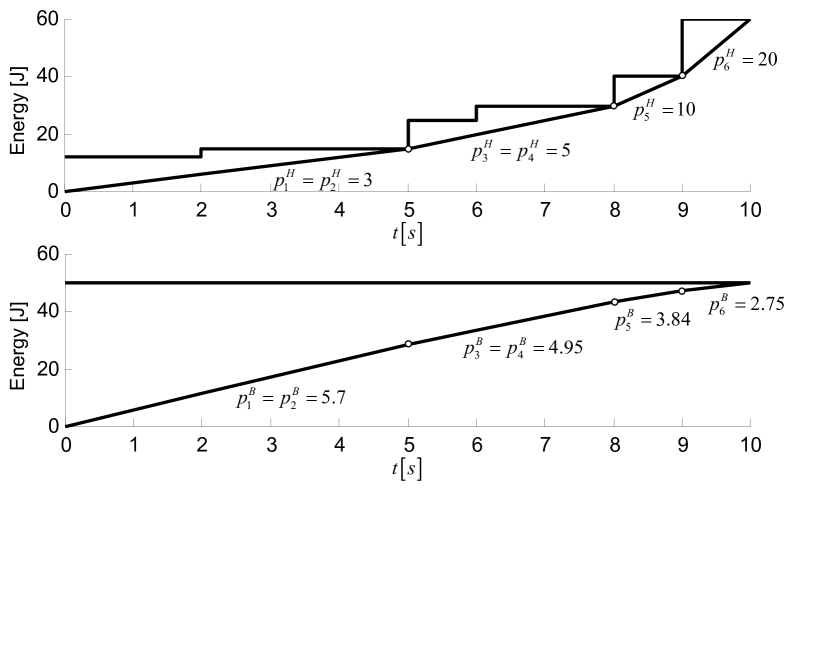
Figure 5: Optimal power allocation: EH and BO sensors ($T=10$, $E_{0}^{2}=50J$)

Finally, Fig. 5 depicts the optimal transmission policies corresponding to the EH and BO sensors for a specific realization of the energy arrivals. Clearly, (i) it satisfies all the lemmas and theorems; (ii) Lemma 4 on the monotonicity of the optimal power allocation does not hold for the BO sensor; and (iii) in order to collaboratively transmit data, the BO sensor must adopt an optimal transmission policy which is different from that of the single-sensor scenario, that is, constant transmit power within $[0\dots T]$.

4.1 Computational complexity analysis

To recall, the computation of the optimal transmission policy for the EH sensor entails the determination of a number of piece-wise linear functions with minimal slope which connect a subset of the $N$ corner points on the cEH curve (see proof of Theorem 1 and [1]). In the worst case, the total number of corner points on the EC curve equals $N$. For the first corner point (actually, the origin), the total number of slopes to be checked equals $N$, that is, as many as the number of corner points up to $t=T$. For the second corner point, the total number of slopes equals $N-1$. The total number of operations is, thus, $N+(N-1)+\ldots 1=\frac{N\cdot(N-1)}{2}$. Hence, the complexity associated to the computation of the optimal transmission policy for the EH sensor is $\mathcal{O}(N^{2})$. As for the BO sensor, each iteration of Algorithm 1 entails the computation of $N$ transmit powers (Steps 6 to 10). When a bi-section scheme is adopted (rather than the grid search we actually used in Algorithm 1), the total number of iterations needed is on the order of $\log(\frac{1}{\epsilon})$ [13], where $\epsilon$ denotes the constraints prescribed tolerance. Hence, the complexity associated to the computations of the optimal transmission policy for the BO sensor is $\mathcal{O}(N\log(\frac{1}{\epsilon}))$. In conclusion, the computational complexity of the proposed scheme is dominated by that of the algorithm presented in [1] and it reads $\mathcal{O}(N^{2})$.

5 Generalization to scenarios with finite storage capacity

Unlike in previous sections, here we assume that the energy storage capacity of the EH sensor, $E_{\text{max}}$, is finite. If, in the $k$-th event, the energy harvested by the EH sensor $E_{k}^{1}$ exceeds the remaining storage capacity at that time instant, a battery overflow occurs. That is, its re-chargeable battery gets fully charged and the excess harvested energy is simply discarded. In Appendix C, we prove that any transmission policy allowing battery overflows to occur is strictly suboptimal. Assuming that $E_{k}^{1}\leq E_{\text{max}}$ $\forall k$, those suboptimal solutions can be removed from the feasible set by imposing that

$$e^{H}\!(t)\geq E^{S}\!(t)\triangleq\sum_{k:s_{k}<t}E_{k}^{1}-E_{\text{max}}$$ (10)

for $0\leq t\leq T$, where $E^{S}\!(t)$ denotes the cumulative energy storage (cES) constraint. One can easily verify that Lemmas 1-3 and Lemma 5 still hold for the case of finite storage capacity. On the contrary, Lemma 4 does not, as we will discuss in the proof of Lemma 7. Since, in particular, Lemma 1 does hold, the optimization problem can be posed again by the set of equations given by (5)-(9) in Section 4, along with the additional constraint (10), namely,

$$\sum_{k=1}^{n}\tau_{k}p_{k}^{H}\geq E_{n}^{S}=\sum_{k=0}^{n}E_{k}^{1}-E_{\text{max}}\;\text{for}\;n=1\ldots N.$$ (11)

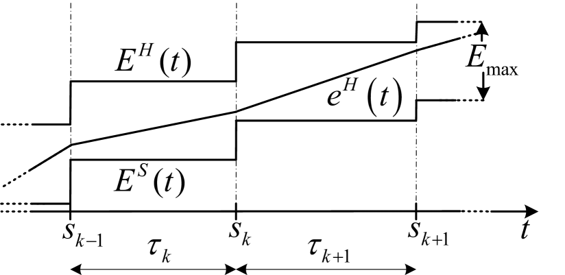
Figure 6: Cumulative energy harvesting and energy storage constraints.

A graphical representation for this additional constraint can be found in Fig. 6. Clearly, a transmit policy is now feasible when the corresponding EC curve lies inside the tunnel defined by the cEH and cES curves. The additional constraint (11) is affine and therefore the optimization problem continues to be convex.

The next Lemma is an extension of Lemma 6 for the case of finite storage capacity:

Lemma 7.

The jointly optimal power allocation policy when the storage capacity of the EH sensor is finite is such that, whenever the transmit power changes, its re-chargeable battery is either fully charged or completely depleted.

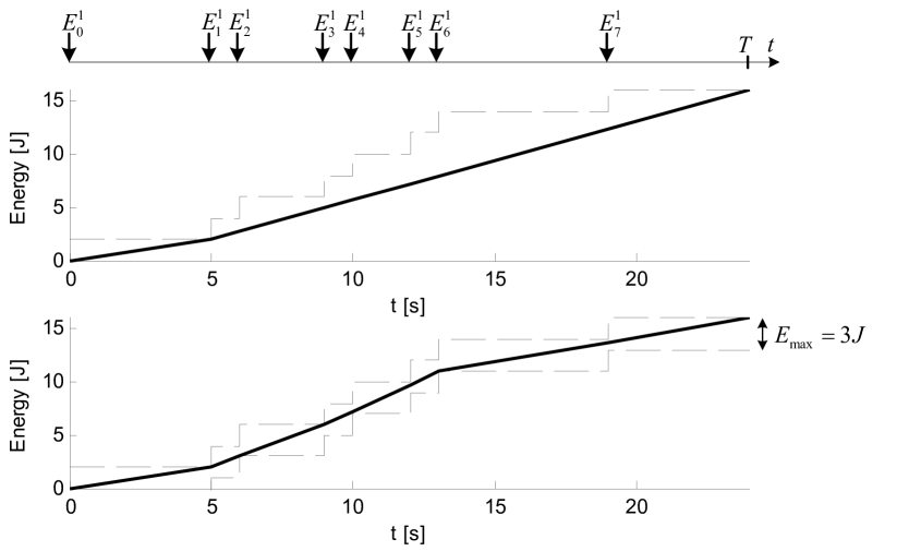
Figure 7: Optimal transmission policy for the EH sensor with infinite (top) and finite (bottom) battery capacity.

Proof.

The proof of this Lemma is based again on the Karush-Kuhn-Tucker (K.K.T.) conditions associated to the new optimization problem and it can be found in Appendix D. This Lemma can also be regarded as an extension of Lemma 4 in [2] for scenarios with multiple sensor nodes forming a virtual array. In essence, Lemma 7 states that changes in the slope of the EC curve can only occur when it hits either the cEH curve (depleted battery) or the cES curve (fully charged). Intuitively, this is the reason why Lemma 4 (on the monotonically increasing behavior of transmit powers for the EH sensor) does not hold anymore in scenarios with finite energy storage capacity. This extent is illustrated in Fig. 7. ∎

In the same vein of Theorem 1, one can easily verify that Lemmas 1-3, 5, and 7 unequivocally determine the optimal transmission policy for the EH harvesting sensor with finite storage capacity. Since those Lemmas are equivalent to the ones presented in [2] for the single sensor case, the (jointly) optimal transmission policy for the EH sensor here can be again independently computed on the basis of algorithm A1 proposed therein. Interestingly, the optimal EC curve turns out to be the shortest feasible string which, now, lies inside the tunnel given by the cEH and cES curves. Besides, the equation in Step 8 of Algorithm 1 in our paper continues to provide a connection between the primal and dual solutions of the problem with finite storage capacity (yet with a different definition of variables $A_{k}$, see Appendix D). Since no additional constraints apply to the BO sensor, its optimal transmission policy can be computed from that of the EH one with Algorithm 1.

6 Computer Simulation Results

In this section, we assess the performance of the proposed power allocation algorithm in a scenario where solar energy is harvested from the environment. The energy storage system in the EH sensor comprises (i) a supercapacitor [14]; and (ii) a re-chargeable Lithium-Ion battery. Upon being harvested, the energy is temporarily stored in the supercapacitor. When it is fully charged, the energy is transferred to the battery in a burst. Clearly, this validates the event-based model of the energy harvesting process presented in Section 2. For such devices, the amount of energy harvested in each event is constant and it equals the maximum energy that can be stored in the supercapacitor. Since solar irradiation levels change over time (e.g. from dawn to noon, from winter to summer), so does the average number of energy arrivals (events). Consequently, the stochastic process that models energy arrivals is non-stationary. In the sequel, we adopt a Poisson process with time-varying mean given by $\lambda_{E}(t)$. From the solar irradiation data in [16], the mean arrival rate from 5 A.M. to 12 P.M. (i.e. dawn to noon, with $T=7$ h) can be fitted by the following exponential function:

$$\lambda_{E}(t)=\beta_{E,c,T}e^{ct}$$ (12)

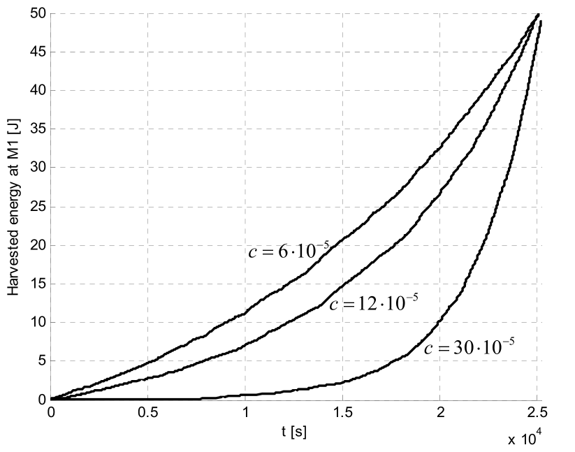
Figure 8: Typical cumulative energy curves parameterized by $c$.

where parameter $c$ models the variability of the energy harvested over time (i.e. the rate of energy transfers from the capacitor to the battery); and $\beta_{E,c,T}$ is a constant depending on the total amount of energy harvested $E$, parameter $c$, and the total harvesting time $T$. For the solar irradiation data in [16], it yields $\beta_{E,c,T}=3.899\cdot 10^{-2}$ and $c=6\cdot 10^{-5}$. Figure 8 shows a number of cumulative energy harvesting curves for different values of parameter $c$: the higher $c$, the higher the energy variability, i.e. the steeper the curves by the end of the observation interval. Hereinafter, we let $E_{T}^{H}=\sum_{k=0}^{N-1}E_{k}^{1}$ and $E_{T}^{B}=E_{0}^{2}$ denote the total energy harvested by/stored in the EH and BO sensors, respectively; whereas $E_{T}=E_{T}^{H}+E_{T}^{B}$ accounts for the total energy in the system. Further, we define $R_{E}={E_{T}^{B}}/{E_{T}^{H}}$ as the ratio between the total energy in the BO and EH sensors, that is, for large $R_{E}$, the battery operated sensor dominates. In all plots, we have $T=7$ h (from 5 A.M. to noon).

6.1 Infinite Energy Storage Capacity

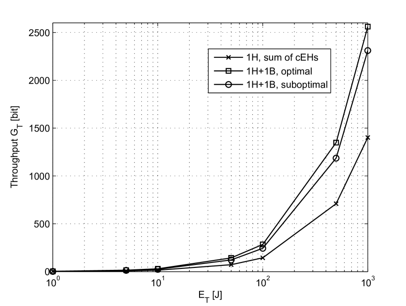
Figure 9: Throughput vs. total energy in the system ($c=30\cdot 10^{-5}$, $R_{E}=1$).

Initially, we assume that the storage capacity of the aforementioned Lithium-ion battery is infinite. In Fig. 9, we depict the throughput of the virtual array with the jointly optimal transmission policies defined by Theorem 1 and Theorem 2 for the EH and BO sensors, respectively. The amount of energy harvested by/stored in the EH and BO sensors is identical ($R_{E}=1$) and results are shown as a function of the total energy $E_{T}$ in the system. As benchmarks, we consider (i) a system with only one EH sensor, the cEH curve of which is given by the point-wise sum of the cEH curves for the EH and BO sensors in the virtual array (curve labeled with “1H, sum of cEHs”); and (ii) a two-sensor virtual array in which the transmission policies for the EH and BO sensors are optimized individually for each sensor as in [1], which is suboptimal for a virtual array (“1H+1B, suboptimal”). For (ii), the optimal policy for the BO sensor consists in a constant transmit power for $t=0\ldots T$. Unsurprisingly, for systems with multiple transmitters the beamforming gain translates into substantially higher throughputs. Besides, some additional throughput gain results from the joint optimization of the transmission policies for the EH and BO sensors, that is, by forcing the BO sensor to adapt to the changes in transmit power in the EH sensor.

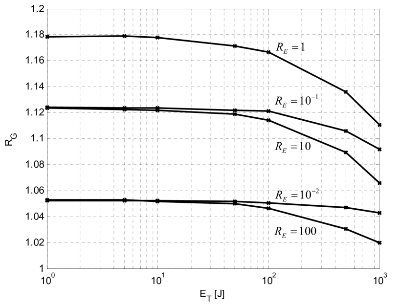
Figure 10: Throughput gain vs. total energy in the system ($c=30\cdot 10^{-5}$).

Fig. 10 provides further insights on the throughput gains stemming from the joint optimization of transmission policies over sensors. More precisely, we depict the throughput gain by ratio $R_{G}={G_{T,\text{opt}}}/{G_{T,\text{subopt}}}$ as a function of the total system energy. Interestingly, the highest gain is attained when the total energy harvested by the EH sensor equals that stored in the BO one, that is, for $R_{E}=1$. Yet in a totally different context, this is consistent with [10] where the authors conclude that, in order to maximize the beamforming gain, the received signal levels from the opportunistically selected sensors must be comparable. Conversely, when either the EH or the BO sensors dominate ($R_{E}\ll 1$ or $R_{E}\gg 1$, respectively) the gain from a joint optimization becomes marginal ($R_{G}\rightarrow 1$) since the signal received from the other sensor is weak. We also observe that, in the case of unbalanced energy levels, throughput gains are lower when the BO sensor dominates. This is motivated by the fact that when $E_{T}^{H}\ll E_{T}^{B}$ the policy for the EH sensor has very little impact in the definition of the (jointly) optimal policy for the BO one. In other words, the energy consumption curves for the BO sensor with and without joint optimization are similar and, hence, the throughput gain approaches 1. It is also clear that throughput gains become negligible when $E_{T}$ increases (i.e. in the high SNR regime). Let $\alpha=E_{T,\text{high}}/E_{T,\text{low}}$ denote the ratio of total system energies in the high and low SNR regimes. Since the total received power $p_{BF}\!(t)$ scales with $\alpha$, from the score function in (5) and for large $E_{T,\text{high}}$ we can write,

$$R_{G}(E_{T,\text{high}})=\frac{N\log(\alpha)+G_{T,\text{opt}}(E_{T,\text{low}})}{N\log(\alpha)+G_{T,\text{subopt}}(E_{T,\text{low}})}.$$

Clearly, for large $\alpha$ the impact of the specific transmission policies (optimal/ suboptimal) diminishes. In other words, joint optimization of transmission policies is more relevant in the low-SNR regime.

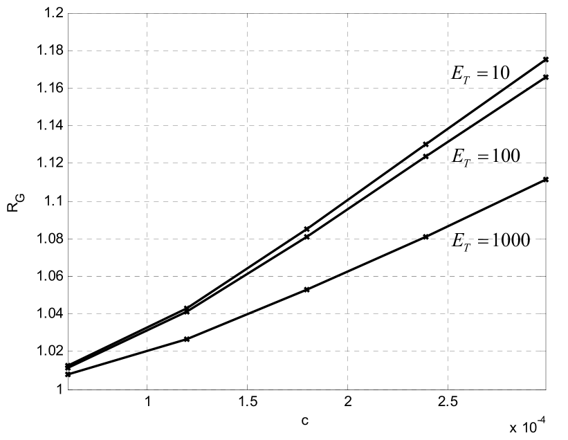
Figure 11: Throughput gain vs. variability of the energy harvested ($R_{E}=1$).

Next, Fig. 11 illustrates the impact of the variability of energy arrivals in the throughput gain. Clearly, the higher the variability (i.e. for higher values of parameter $c$), the higher the gain: $R_{G}=1.2$ (or $+20\%$ gain) for $c=3\cdot 10^{-4}$ and $E_{T}=10$ J. On the contrary, if the average number of arrivals does not vary (increase) substantially in the observation interval, the gain stemming from a joint optimization of both transmission policies is marginal ($R_{G}\approx 1$). In conclusion, rapid variations of solar irradiation levels from dawn to noon (e.g. in high latitude locations, winter time) make joint optimization of transmission policies advisable.

6.2 Finite Energy Storage Capacity

Unlike in the previous subsection, here we realistically assume that the energy storage capacity for the EH sensor is finite.

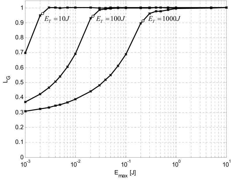
Figure 12: Throughput ratio (loss) as a function of battery capacity ($N=2250$ epochs). Big round markers on the curve correspond to the operating points where the maximum storage capacity $E_{\text{max}}$ equals the energy harvested in each arrival $E_{k}^{1}$ ($E_{k}^{1}=2.21\cdot 10^{-3},2.21\cdot 10^{-2},2.21\cdot 10^{-1}$ for the $E_{T}=10,100,1000$ J curves, respectively).

Figure 12 depicts the total loss in throughput with respect to the case of infinite storage capacity by throughpout ratio $L_{G}$. Interestingly, as long as the maximum storage capacity is greater than the energy harvested in each arrival, the throughput loss is barely noticeable (the throughput ratio equals 1). In other words, the changes in the optimal transmission policy resulting from the introduction of the additional constraint (11), which avoids battery overflows, have a rather marginal impact on the achievable throughput. This is excellent news since, typically, storage capacity is well above individual harvested energy levels. On the contrary, throughput performance rapidly degrades for smaller storage capacities. This stems from the fact that now part of the energy in each arrival is unavoidably wasted in battery overflows. As a result, the total amount of energy stored with respect to the case of infinite capacity decreases, and so does the resulting throughput.

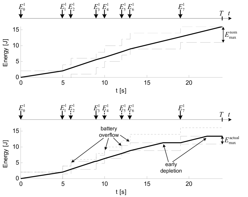
Figure 13: Battery overflow and early depletion phenomena: transmission policies for the EH sensor with nominal battery capacity (top, $E_{\text{max}}^{\text{nom}}=5$ J) and actual capacity (bottom, $E_{\text{max}}^{\text{actual}}=2.5$ J) for a given realization of energy arrivals. Dotted arrows indicate the arrivals in which part of the energy is wasted ($E_{k}^{1}=2$ J). As a reference, the lower plot includes the cEH curve for the nominal capacity (dash-dotted line).

Next, we analyze the impact of battery degradation in the EH sensor on system performance. Our focus is on impairments due to long-term battery degradation due to e.g. aging. Accordingly, its storage capacity is assumed to take a constant value for the whole transmission period (i.e. no battery leakage between arrivals). The nominal storage capacity $E_{\text{max}}^{\text{nom}}$, on which basis the optimal transmission policies for the EH and BO are computed, is assumed to be known. On the contrary, the actual capacity $E_{\text{max}}^{\text{actual}}\leq E_{\text{max}}^{\text{nom}}$, which enables data transmission, is unknown. The fact that the actual capacity is lower that its nominal value may result into battery overflows and early battery depletion (see Fig. 13), both having a negative impact on the achievable throughput. Despite of the introduction of the additional constraint (11), now there is a risk to waste part of the energy arrivals in battery overflows since the remaining battery capacity is smaller than expected. As an example, for the particular realization in Fig. 13, the total energy actually harvested within $0\ldots T$ amounts to $13.375$ J instead of $16$ J. Likewise, the fact that the actual energy stored in the battery is lower than expected might lead to early battery depletions. This forces data transmission for the EH sensor to be suspended until the next energy arrival. Consequently, the beamforming gain vanishes for this period of time.

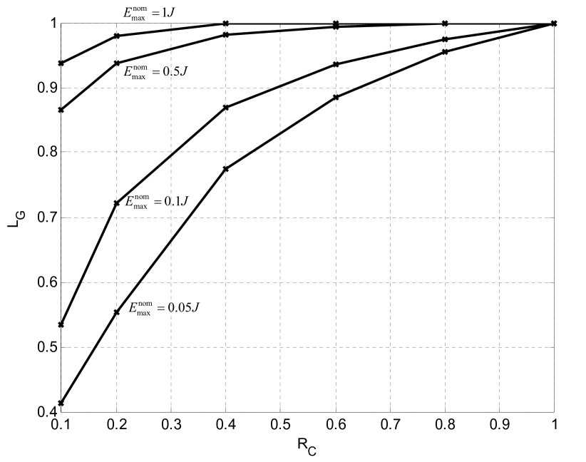
Figure 14: Throughput ratio (loss) due to battery capacity degradation ($E_{T}=100$ J, $c=30\cdot 10^{-5}$, $T=7h$)

In Fig. 14, we investigate the impact of battery overflows and early depletions on throughput. More specifically, we depict the throughput ratio $L_{G}={G_{T,\text{actual}}}/{G_{T,\text{nom}}}$ as a function of the ratio between actual and nominal battery capacities, namely, $R_{C}={E_{\text{max}}^{\text{actual}}}/{E_{\text{max}}^{\text{nom}}}$. Unsurprisingly, throughput degradation is particulary severe and faster for smaller values of nominal capacity (i.e. for $E_{\text{max}}^{\text{nom}}=0.05$ J). In this case, the amount of energy in each arrival ($E_{k}^{1}=2.21\cdot 10^{-2}$ J) is comparable to the nominal capacity. Consequently, many battery overflows and early depletions occur. Furthermore, for $R_{C}=0.1$, the actual battery capacity amounts to $E_{\text{max}}^{\text{actual}}=5\cdot 10^{-3}$ which is below $E_{k}^{1}$. Hence, every energy arrival causes a battery overflow which results into a throughput loss of $60\%$. It is also worth noting that for large nominal battery capacities ($E_{\text{max}}^{\text{nom}}=1$ J) and higher values of capacity degradation ($R_{C}=0.1$) there is also a noticeable throughput loss (some $10\%$). Even though the actual battery capacity ($E_{\text{max}}^{\text{actual}}=0.1$ J) is well above $E_{k}^{1}$, the mismatch between nominal and actual capacities results into some battery overflows and early depletions too.

7 Conclusions

In this paper, we have derived the jointly optimal transmission policy which allows an energy harvesting plus a battery operated sensor node to act as a virtual antenna array to maximize throughput for a given deadline. The necessary conditions for optimality that we have identified, both for scenarios with infinite and finite energy storage capacity in the energy harvesting sensor, allowed us to prove that the optimal transmission policy for the energy harvesting sensor can be computed independently from that of the battery operated one according to the procedure described in [1] and [2], respectively. Interestingly enough, we have proved that such policies continue to be optimal for our two-sensor (vs. single-sensor) scenario. Moreover, we have shown that the optimal transmission policy for the battery operated sensor is unequivocally determined and can be iteratively computed from that of the energy harvesting one. The resulting policy is, in general, different from that of battery operated sensors in single-sensor scenarios (i.e. constant transmit power). The performance of the jointly optimal transmission policy has been assessed by means of computer simulations in a realistic scenario where solar energy is harvested from the environment. Computer simulation results revealed that, in scenarios with infinite storage capacity in the energy harvesting sensor, the joint optimization of transmit policies in combination with beamforming yields substantial throughput gains. The highest gain is attained when the total energy in the energy harvesting and battery operated sensors are identical. However, the gain becomes negligible in high-SNR scenarios where large amounts of energy are harvested by/stored in sensors. In the case of unbalanced energy levels, throughput gains are lower when the BO sensor dominates. Besides, we have found that throughput gain is larger when solar irradiation levels vary rapidly. We have also learnt that throughput losses stemming from finite storage capacity are only substantial when battery capacity is smaller than the amount of energy in each arrival. Finally, we have observed that a long-term degradation of battery capacity may result into battery overflows and early battery depletions. The associated throughput loss is particulary severe for smaller values of the nominal storage capacity. Still, the impact of the mismatch between nominal and actual capacities can also be noticeable for larger values.

8 Acknowledgements

This work is partly supported by the project JUNTOS (TEC2010-17816), NEWCOM# (318306), Spanish Ministry of Education (FPU grant AP2008-03952) and by the Catalan Government under 2009 SGR 1046.

Appendix A Proof of Lemma 1

Assume that the optimal policy before $s_{k-1}$ and after $s_{k}$ is optimal. The total throughput in the $k$-th epoch is given by $G_{\tau_{k}}=\int_{s_{k-1}}^{s_{k}}\log(1+p_{BF}(t))dt$ where, to recall, we defined $p_{BF}\!(t)=(\sqrt{p^{H}\!(t)}+\sqrt{p^{B}\!(t)})^{2}$ as the instantaneous power received at the base station from the two sensors. Besides, let $\Delta e_{BF}=\int_{s_{k-1}}^{s_{k}}p_{BF}(t)dt$ denote the total received energy in the $k$-th epoch of duration $\tau_{k}=s_{k}-s_{k-1}$. From Jensen’s inequality [17][Sec. 7.2.5], we have that the following inequality:

$$\frac{\int_{a}^{b}g\left(f(t)\right)h(t)dt}{\int_{a}^{b}h(t)dt}\leq g\left(\frac{\int_{a}^{b}f(t)h(t)dt}{\int_{a}^{b}h(t)dt}\right)\\$$

holds as long as $g(\cdot)$ is a concave function, $f(t)$ is such that $\alpha\leq f(t)\leq\beta$, and $h(t)\geq 0$. Letting $g(p)=\log(1+p)$, $f(t)=p_{BF}(t)$ and $h(t)=1$ yields

$$G_{\tau_{k}} =\int_{s_{k-1}}^{s_{k}}\log(1+p_{BF}(t))dt$$

$$\leq\tau_{k}\log\left(1+\left(\frac{\int_{s_{k-1}}^{s_{k}}p_{BF}(t)dt}{\int_{s_{k-1}}^{s_{k}}dt}\right)\right)$$ (13)

$$=\tau_{k}\log\left(1+\frac{\Delta e_{BF}}{\tau_{k}}\right).$$

This last inequality evidences that for a given energy $\Delta e_{BF}$, the optimal power allocation policies for the $k$-th epoch must be such that the instantaneous received power at the BS is constant and equal to $p_{BF}(t)=\Delta e_{BF}/\tau_{k}$. In order to determine the optimal transmission policy for each sensor, we resort to Cauchy’s inequality [17][Sec. 7.2.5] to learn that

$$\left(\int_{s_{k-1}}^{s_{k}}p_{BF}(t)dt\right)^{\frac{1}{2}}\leq\left(\int_{s_{k-1}}^{s_{k}}p^{H}\!(t)dt\right)^{\frac{1}{2}}+\left(\int_{s_{k-1}}^{s_{k}}p^{B}\!(t)dt\right)^{\frac{1}{2}}$$

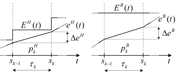
Figure 15: Transmit power in each sensor remains constant between consecutive events (Lemma 1).

or, equivalently (see Fig. 15),

$$\int_{s_{k-1}}^{s_{k}}p_{BF}(t)dt\leq\left(\sqrt{\Delta e^{H}}+\sqrt{\Delta e^{B}}\right)^{2}.$$ (14)

By replacing (14) into (13), we finally get:

$$G_{\tau_{k}}\leq\tau_{k}\log\left(1+\left(\sqrt{\frac{\Delta e^{H}}{\tau_{k}}}+\sqrt{\frac{\Delta e^{B}}{\tau_{k}}}\right)^{2}\right).$$ (15)

In other words, the individual power allocation policies that maximize the throughput in the $k$-th epoch consist in using a constant transmit power given by $p^{H}\!(t)=\Delta e^{H}/\tau_{k}$ and $p^{B}\!(t)=\Delta e^{B}/\tau_{k}$ for the EH and BO sensors, respectively. This concludes the proof.

Appendix B Proof of Lemma 6

The Lagrangian of the optimization problem (9) is given by

$$\mathcal{L}_{1}= -\sum_{k=1}^{N}\tau_{k}\log\left(1+(\sqrt{p^{H}_{k}}+\sqrt{p^{B}_{k}})^{2}\right)$$

$$+\sum_{n=1}^{N}\lambda_{n}\left(\sum_{k=1}^{n}\tau_{k}p^{H}_{k}-E_{n}^{H}\right)+\sum_{n=1}^{N}\nu_{n}\left(\sum_{k=1}^{n}\tau_{k}p^{B}_{k}-E_{n}^{B}\right)$$

$$-\sum_{k=1}^{N}\mu_{k}p^{H}_{k}-\sum_{k=1}^{N}\xi_{k}p^{B}_{k}$$ (16)

and, hence, the corresponding K.K.T. conditions read

$$\frac{\partial\mathcal{L}_{1}}{\partial p^{H}_{k}},\frac{\partial\mathcal{L}_{1}}{\partial p^{B}_{k}} =0$$ (17)

$$\sum_{k=1}^{n}\tau_{k}\breve{p}^{H}_{k} \leq E_{n}^{H}\;\text{for}\;n=1\ldots N$$ (18)

$$\sum_{k=1}^{n}\tau_{k}\breve{p}^{B}_{k} \leq E_{n}^{B}\;\text{for}\;n=1\ldots N$$ (19)

$$\breve{p}^{H}_{k},\breve{p}^{B}_{k} >0$$ (20)

$$\breve{\lambda}_{n},\breve{\nu}_{n},\breve{\mu}_{k},\breve{\xi}_{k} \geq 0$$ (21)

$$\breve{\lambda}_{n}\left(\sum_{k=1}^{n}\tau_{k}\breve{p}^{H}_{k}-E_{n}^{H}\right) =0\;\text{for}\;n=1\ldots N$$ (22)

$$\breve{\nu}_{n}\left(\sum_{k=1}^{n}\tau_{k}\breve{p}^{B}_{k}-E_{n}^{B}\right) =0\;\text{for}\;n=1\ldots N$$ (23)

$$-\breve{\mu}_{k}\breve{p}^{H}_{k} =0\;\text{for}\;k=1\ldots N$$ (24)

$$-\breve{\xi}_{k}\breve{p}^{B}_{k} =0\;\text{for}\;k=1\ldots N.$$ (25)

where the partial derivatives in (17) are can be expressed as

$$\frac{\partial\mathcal{L}_{1}}{\partial p^{H}_{k}}=-\tau_{k}\frac{\sqrt{\breve{p}^{H}_{k}}+\sqrt{\breve{p}^{B}_{k}}}{\sqrt{\breve{p}^{H}_{k}}\left(1+(\sqrt{\breve{p}^{H}_{k}}+\sqrt{\breve{p}^{B}_{k}})^{2}\right)}+\tau_{k}\sum_{n=k}^{N}\breve{\lambda}_{n}-\breve{\mu}_{k}$$

$$\frac{\partial\mathcal{L}_{1}}{\partial p^{B}_{k}}=-\tau_{k}\frac{\sqrt{\breve{p}^{H}_{k}}+\sqrt{\breve{p}^{B}_{k}}}{\sqrt{\breve{p}^{B}_{k}}\left(1+(\sqrt{\breve{p}^{H}_{k}}+\sqrt{\breve{p}^{B}_{k}})^{2}\right)}+\tau_{k}\sum_{n=k}^{N}\breve{\nu}_{n}-\breve{\xi}_{k}$$

From equation (17) and by introducing the change of variables $\breve{A}_{k}=\sum_{n=k}^{N}\breve{\lambda}_{n}-\frac{\breve{\mu}_{k}}{\tau_{k}}$ and $\breve{B}_{k}=\sum_{n=k}^{N}\breve{\nu}_{n}-\frac{\breve{\xi}_{k}}{\tau_{k}}$, the optimal transmit powers in $k$-th epoch, $\breve{p}^{H}_{k}$ and $\breve{p}^{B}_{k}$, yield

$$\breve{p}^{H}_{k}=\frac{\breve{B}_{k}(\breve{A}_{k}+\breve{B}_{k}-\breve{A}_{k}\breve{B}_{k})}{\breve{A}_{k}(\breve{A}_{k}+\breve{B}_{k})^{2}}$$ (26)

$$\breve{p}^{B}_{k}=\frac{\breve{A}_{k}(\breve{A}_{k}+\breve{B}_{k}-\breve{A}_{k}\breve{B}_{k})}{\breve{B}_{k}(\breve{A}_{k}+\breve{B}_{k})^{2}}.$$ (27)

Since, as stated in Lemma 5 and equation (20) above, $\breve{p}^{H}_{k},\breve{p}^{B}_{k}\neq 0$, the complementary slackness conditions (24) and (25), force the corresponding Langrangian multipliers to vanish, i.e. $\breve{\mu}_{k},\breve{\xi}_{k}=0$. When transmit power changes, we have $\breve{p}^{H}_{k}<\breve{p}^{H}_{k+1}$. From (26) and the Remark below, this can only hold if $\breve{A}_{k}\neq\breve{A}_{k+1}$ or, equivalently, if $\breve{\lambda}_{k}\neq 0$ (to recall, $\breve{\mu}_{k}=0$). From the complementary slackness condition in (22), we have that $\breve{\lambda}_{k}\neq 0\Rightarrow\sum_{i=1}^{k}\tau_{i}{\breve{p}^{H}_{i}}-E_{k}^{H}=0$. That is, the energy consumed by the energy harvesting sensor up to $s_{k}$, equals the energy harvested by such sensor up to that instant (see Fig. 16). This concludes the proof.

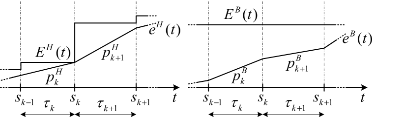
Figure 16: When transmit power changes, the energy consumed by the EH sensor equals the energy harvested (Lemma 6).

Remark: From Lemma 2, we know that $\sum_{k=1}^{N}\tau_{k}\breve{p}^{B}_{k}=E_{0}^{2}$. Since, in addition $\breve{p}^{B}_{k}\neq 0$ this yields $\sum_{k=1}^{n}\tau_{k}\breve{p}^{B}_{k}-E_{0}^{2}<0$ for all $n=1\ldots N-1$. From the complementary slackness condition of (23), we conclude that, necessarily, $\breve{\nu}_{k}=0$ for $k=1\ldots N-1$. This, along with the fact that $\breve{\mu}_{k}=0$ for all $k$, implies that $\breve{B}_{k}=\breve{B}_{N}=\nu_{N},\forall k$, that is, all $\breve{B}_{k}$s are identical. This property is a cornerstone of Algorithm 1 since it turns an $N$-dimensional exhaustive search into a single-dimensional one.

Appendix C Transmission policies with battery overflows are suboptimal

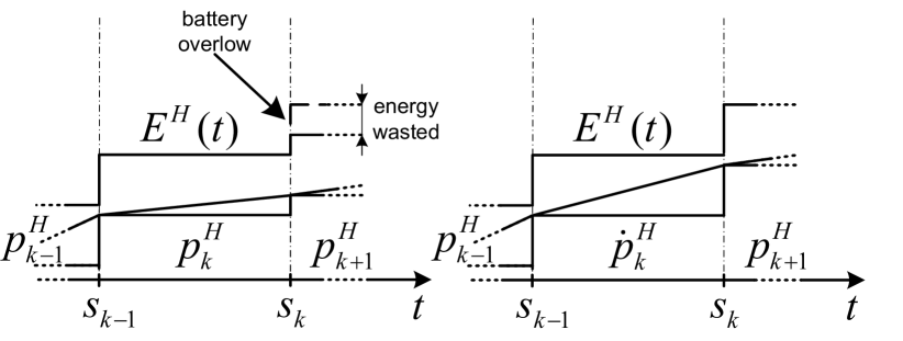
Figure 17: Transmission policies with battery overflows are strictly suboptimal.

Here we show that any transmission policy resulting into battery overflows in the EH sensor is strictly suboptimal. We will prove this by contradiction. Assume that a transmission policy with battery overflow at $s_{k}$ only (Fig. 17 left) is optimal. Let ${\Pi}^{H}=\{p_{1}^{H},\ldots,p_{k-1}^{H},{p}_{k}^{H},p_{k+1}^{H},\dots,p_{N}^{H}\}$ and ${\Pi}^{B}=\{{p}_{1}^{B},\ldots,{p}_{k-1}^{B},{p}_{k}^{B},{p}_{k+1}^{B},\dots,{p}_{N}^{B}\}$ denote the corresponding optimal transmission policies for the EH and BO sensors, respectively. We can think of an alternative (and feasible) transmission policy $\dot{\Pi}=\{\dot{\Pi}^{H},\dot{\Pi}^{B}\}$ such that, on the one hand, $\dot{\Pi}^{H}=\{p_{1}^{H},\ldots,p_{k-1}^{H},\dot{p}_{k}^{H},p_{k+1}^{H},p_{N}^{H}\}$ and, on the other, $\dot{\Pi}^{B}={\Pi}^{B}$. That is, the new policy only differs from the optimal one in the power allocated to the EH sensor in the $k$-th epoch. By properly adjusting $\dot{p}_{k}^{H}$, the battery overflow at $s_{k}$ can be avoided (Fig. 17 right). Since, clearly, $\dot{p}_{k}^{H}>{p}_{k}^{H}$, the throughput in the $k$-th epoch is higher, this resulting into a higher total throughput in $[0\ldots T]$. This contradicts the claim that the original policy ${\Pi}=\{{\Pi}^{H},{\Pi}^{B}\}$ is optimal and concludes the proof.

Appendix D Proof of Lemma 7

The Lagrangian $\mathcal{L}_{2}$ of the new optimization problem with finite battery capacity constraints is given by

$$\mathcal{L}_{2}= -\sum_{k=1}^{N}\tau_{k}\log\left(1+(\sqrt{p^{H}_{k}}+\sqrt{p^{B}_{k}})^{2}\right)$$

$$+\sum_{n=1}^{N}\lambda_{n}\left(\sum_{k=1}^{n}\tau_{k}p^{H}_{k}-E_{n}^{H}\right)-\sum_{n=1}^{N}\pi_{n}\left(\sum_{k=1}^{n}\tau_{k}p_{k}^{H}-E_{n}^{S}\right)$$

$$+\sum_{n=1}^{N}\nu_{n}\left(\sum_{k=1}^{n}\tau_{k}p^{B}_{k}-E_{n}^{B}\right)-\sum_{k=1}^{N}\mu_{k}p^{H}_{k}-\sum_{k=1}^{N}\xi_{k}p^{B}_{k}.$$ (28)

The new K.K.T. conditions thus read

$$\frac{\partial\mathcal{L}_{2}}{\partial p^{H}_{k}},\frac{\partial\mathcal{L}_{2}}{\partial p^{B}_{k}} =0$$ (29)

$$\sum_{k=1}^{n}\tau_{k}\breve{p}^{H}_{k} \leq E_{n}^{H}\;\text{for}\;n=1\ldots N$$ (30)

$$\sum_{k=1}^{n}\tau_{k}\breve{p}^{H}_{k} \geq E_{n}^{S}\;\text{for}\;n=1\ldots N$$ (31)

$$\sum_{k=1}^{n}\tau_{k}\breve{p}^{B}_{k} \leq E_{n}^{B}\;\text{for}\;n=1\ldots N$$ (32)

$$\breve{p}^{H}_{k},\breve{p}^{B}_{k} >0$$ (33)

$$\breve{\lambda}_{n},\breve{\pi}_{n},\breve{\nu}_{n},\breve{\mu}_{k},\breve{\xi}_{k} \geq 0$$ (34)

$$\breve{\lambda}_{n}\left(\sum_{k=1}^{n}\tau_{k}\breve{p}^{H}_{k}-E_{n}^{H}\right) =0\;\text{for}\;n=1\ldots N$$ (35)

$$\breve{\pi}_{n}\left(\sum_{k=1}^{n}\tau_{k}\breve{p}^{H}_{k}-E_{n}^{S}\right) =0\;\text{for}\;n=1\ldots N$$ (36)

$$\breve{\nu}_{n}\left(\sum_{k=1}^{n}\tau_{k}\breve{p}^{B}_{k}-E_{n}^{B}\right) =0\;\text{for}\;n=1\ldots N$$ (37)

$$-\breve{\mu}_{k}\breve{p}^{H}_{k} =0\;\text{for}\;k=1\ldots N$$ (38)

$$-\breve{\xi}_{k}\breve{p}^{B}_{k} =0\;\text{for}\;k=1\ldots N$$ (39)

where equation (36) accounts for the additional constraint given by (11), and $\{\pi_{n}\}$ denote the corresponding set of Lagrange multipliers. Since the additional constraint does not apply to the BO sensor, the partial derivative $\frac{\partial\mathcal{L}_{2}}{\partial p^{B}_{k}}$ is identical to that in Appendix B, namely, $\frac{\partial\mathcal{L}_{2}}{\partial p^{B}_{k}}=\frac{\partial\mathcal{L}_{1}}{\partial p^{B}_{k}}$. On the contrary, $\frac{\partial\mathcal{L}_{2}}{\partial p^{H}_{k}}$ differs and, more specifically, it reads

$$\frac{\partial\mathcal{L}_{2}}{\partial p^{H}_{k}}=-\tau_{k}\frac{\sqrt{\breve{p}^{H}_{k}}+\sqrt{\breve{p}^{B}_{k}}}{\sqrt{\breve{p}^{H}_{k}}\left(1+(\sqrt{\breve{p}^{H}_{k}}+\sqrt{\breve{p}^{B}_{k}})^{2}\right)}+\tau_{k}(\sum_{n=k}^{N}\breve{\lambda}_{n}-\breve{\pi}_{n})-\breve{\mu}_{k}$$ (40)

From (29) and by introducing the change of variables $\breve{A}_{k}=\sum_{n=k}^{N}(\breve{\lambda}_{n}-\breve{\pi}_{n})-\frac{\breve{\mu}_{k}}{\tau_{k}}$ and $\breve{B}_{k}=\sum_{n=k}^{N}\breve{\nu}_{n}-\frac{\breve{\xi}_{k}}{\tau_{k}}$, the optimal transmit powers in $k$-th epoch, $\breve{p}^{H}_{k}$ and $\breve{p}^{B}_{k}$, again yield

$$\breve{p}^{H}_{k}=\frac{\breve{B}_{k}(\breve{A}_{k}+\breve{B}_{k}-\breve{A}_{k}\breve{B}_{k})}{\breve{A}_{k}(\breve{A}_{k}+\breve{B}_{k})^{2}}$$ (41)

$$\breve{p}^{B}_{k}=\frac{\breve{A}_{k}(\breve{A}_{k}+\breve{B}_{k}-\breve{A}_{k}\breve{B}_{k})}{\breve{B}_{k}(\breve{A}_{k}+\breve{B}_{k})^{2}}.$$ (42)

Equation (33) and the complementary slackness conditions (38) and (39) again force the corresponding Lagrangian multipliers to vanish, i.e. $\breve{\mu}_{k},\breve{\xi}_{k}=0$. As in Appendix B, the transmit power changes ($\breve{p}^{H}_{k}\neq\breve{p}^{H}_{k+1}$) iff $\breve{A}_{k}\neq\breve{A}_{k+1}$ or, equivalently, if $\breve{\lambda}_{k}-\breve{\pi}_{k}\neq 0$. This is only possible for the following combinations of values of the Lagrangian multiplier: (i) $\breve{\lambda}_{k}\neq 0,\breve{\pi}_{k}=0$; (ii) $\breve{\lambda}_{k}=0,\breve{\pi}_{k}\neq 0$; or (iii) $\breve{\lambda}_{k}\neq 0,\breve{\pi}_{k}\neq 0,\breve{\lambda}_{k}\neq\breve{\pi}_{k}$. The conditions (i) and (ii) accounts for cases in which the EC curve hits the cEH or cES curves at $s_{k}$ respectively; whereas (iii) accounts for the case in which the cEH and cES curves coincide at time instant $s_{k}$ (i.e. when energy harvested at $s_{k}$ equals battery capacity, namely, $E_{k}^{1}=E_{\text{max}}$).

References

- Yang and Ulukus [2012] J. Yang, S. Ulukus, Optimal packet scheduling in an energy harvesting communication system, IEEE Transactions on Communications 60 (2012) 220 –230.
- Tutuncuoglu and Yener [2012] K. Tutuncuoglu, A. Yener, Optimum transmission policies for battery limited energy harvesting nodes, IEEE Transactions on Wireless Communications 11 (2012) 1180 –1189.
- Ozel et al. [2011] O. Ozel, K. Tutuncuoglu, J. Yang, S. Ulukus, A. Yener, Transmission with energy harvesting nodes in fading wireless channels: Optimal policies, IEEE Journal on Selected Areas in Communications 29 (2011) 1732 –1743.
- Yang and Ulukus [2012] J. Yang, S. Ulukus, Optimal packet scheduling in a multiple access channel with energy harvesting transmitters, Journal of Communications and Networks 14 (2012) 140 –150.
- Tutuncuoglu and Yener [2012] K. Tutuncuoglu, A. Yener, Sum-rate optimal power policies for energy harvesting transmitters in an interference channel, Journal of Communications and Networks 14 (2012) 151 –161.
- Gunduz and Devillers [2011] D. Gunduz, B. Devillers, Two-hop communication with energy harvesting, in: 4th IEEE International Workshop on Computational Advances in Multi-Sensor Adaptive Processing (CAMSAP), 2011, pp. 201 –204.
- Yang et al. [2012] J. Yang, O. Ozel, S. Ulukus, Broadcasting with an energy harvesting rechargeable transmitter, Wireless Communications, IEEE Transactions on 11 (2012) 571 –583.
- Ozel et al. [2012] O. Ozel, J. Yang, S. Ulukus, Optimal broadcast scheduling for an energy harvesting rechargeable transmitter with a finite capacity battery, Wireless Communications, IEEE Transactions on 11 (2012) 2193 –2203.
- Mudumbai et al. [2010] R. Mudumbai, J. Hespanha, U. Madhow, G. Barriac, Distributed transmit beamforming using feedback control, IEEE Transactions on Information Theory 56 (2010) 411 –426.
- Pun et al. [2008] M.-O. Pun, D. Brown, H. Vincent Poor, Opportunistic collaborative beamforming with one-bit feedback, SPAWC 2008. (2008) 246 –250.
- Berbakov et al. [2012] L. Berbakov, J. Matamoros, C. Anton-Haro, Optimal transmission policy for distributed beamforming with energy harvesting and battery operated sensor nodes, in: 9th International Symposium on Wireless Communication Systems (ISWCS) 2012.
- Devillers and Gunduz [2012] B. Devillers, D. Gunduz, A general framework for the optimization of energy harvesting communication systems with battery imperfections, Communications and Networks, Journal of 14 (2012) 130 –139.
- Burden and Faires [2011] R. L. Burden, J. D. Faires, Numerical Analysis, Brooks/Cole, 2011.
- Saggini et al. [2010] S. Saggini, F. Ongaro, C. Galperti, P. Mattavelli, Supercapacitor-based hybrid storage systems for energy harvesting in wireless sensor networks, in: Applied Power Electronics Conference and Exposition (APEC), 2010 Twenty-Fifth Annual IEEE, pp. 2281 –2287.
- Li et al. [2001] J. Li, E. Murphy, J. Winnick, P. A. Kohl, The effects of pulse charging on cycling characteristics of commercial lithium-ion batteries, Journal of Power Sources 102 (2001) 302 – 309.
- NSR [2005] National solar radiation data base, 1991-2005. http://rredc.nrel.gov/solar/old_data/nsrdb/1991-2005/tmy3/.
- Polyanin and Manzhirov [2007] A. D. Polyanin, A. V. Manzhirov, Handbook of Mathematics for Engineers and Scientists, Chapman & Hall/CRC, 2007.