Convergence and prediction of principal component scores in high-dimensional settings

Abstract

A number of settings arise in which it is of interest to predict Principal Component (PC) scores for new observations using data from an initial sample. In this paper, we demonstrate that naive approaches to PC score prediction can be substantially biased toward 0 in the analysis of large matrices. This phenomenon is largely related to known inconsistency results for sample eigenvalues and eigenvectors as both dimensions of the matrix increase. For the spiked eigenvalue model for random matrices, we expand the generality of these results, and propose bias-adjusted PC score prediction. In addition, we compute the asymptotic correlation coefficient between PC scores from sample and population eigenvectors. Simulation and real data examples from the genetics literature show the improved bias and numerical properties of our estimators.

, and

t1Supported in part by NIH Grant GM074175. t2Supported in part by the Carolina Environmental Bioinformatics Center (EPA RD832720) and a Gillings Innovation Award.

1 Introduction

Principal component analysis (PCA) jolliffe2002pca is one of the leading statistical tools for analyzing multivariate data. It is especially popular in genetics/genomics, medical imaging and chemometrics studies where high-dimensional data is common. PCA is typically used as a dimension reduction tool. A small number of top ranked principal component (PC) scores are computed by projecting data onto spaces spanned by the eigenvectors of sample covariance matrix, and are used to summarize data characteristics that contribute most to data variation. These PC scores can be subsequently used for data exploration and/or model predictions. For example, in genome-wide association studies (GWAS), PC scores are used to estimate ancestries of study subjects and as covariates to adjust for population stratification price2006pca , patterson2006psa . In gene expression microarray studies, PC scores are used as synthetic “eigen-genes” or “meta-genes” intended to represent and discover gene expression patterns that might not be discernible from single-gene analysis wall2003svd .

Although PCA is widely applied in a number of settings, much of our theoretical understanding rests on a relatively small body of literature. Girshick girshick1936principal introduced the idea that the eigenvectors of sample covariance matrix are maximum likelihood estimators. Here, a key concept in a population view of PCA is that the data arise as $p$-variate values from a distinct set of $n$ independent samples. Later, the asymptotic distribution of eigenvalues and eigenvectors of the sample covariance matrix (i.e., the sample eigenvalues and eigenvectors) were derived for the situation where $n$ goes to infinity and $p$ is fixed girshick1939sampling , Anderson1 . With the development of modern high-throughput technologies, it is not uncommon to have data where $p$ is comparable in size to $n$, or substantially larger. Under the assumption that $p$ and $n$ grow at the same rate, that is $p/n\rightarrow\gamma>0$, there has been considerable effort to establish convergence results for sample eigenvalues and eigenvectors (see review bai1999msa ). The convergence of the sample eigenvalues and eigenvectors under the “spiked population” model proposed by Johnstone johnstone2001 has also been established Baik2006 , paul2007 , nadler2008fsa . For this model, it is well known that the sample eigenvectors are not consistent estimators of the eigenvectors of population covariance (i.e., the population eigenvectors) johnstone2007spc , paul2007 , nadler2008fsa . Furthermore, Paul paul2007 has derived the degree of discrepancy in terms of the angle between the sample and population eigenvectors, under Gaussian assumptions for $0<\gamma<1$. More recently, Nadler nadler2008fsa has extended the same result to the more general $\gamma>0$ using a matrix perturbation approach.

These results have considerable potential practical utility in understanding the behavior of PC analysis and prediction in modern datasets, for which $p$ may be large. The practical goals of this paper focus primarily on the prediction of PC scores for samples which were not included in the original PC analysis. For example, gene expression data of new breast cancer patients may be collected, and we might want to estimate their PC scores in order to classify their cancer sub-type. The recalculation of PCs using both new and old data might not be practical. For example, if the application of PCs from gene expression is used as a diagnostic tool in clinical applications. For GWAS analysis, it is known that PC analysis which includes related individuals tends to generate spurious PC scores which do not reflect the true underlying population substructures. To overcome this problem, it is common practice to include only one individual per family/sibship in the initial PC analysis. Another example arises in cross-validation for PC regression, in which PC scores for the test set might be derived using PCA performed on the training set jackson2005user . For all of these applications, the predicted PC scores for a new sample are usually estimated in the “naive” fashion, in which the data vector of the new sample is multiplied by the sample eigenvectors from the original PC analysis. Indeed, there appears to be relatively little recognition in the genetics or data mining literature that this approach may lead to misleading conclusions.

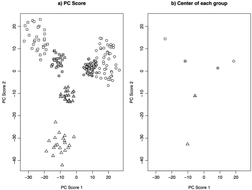
Figure 1: Simulation results for $p=5000$ and $n=(50,30,20)$. Different symbols represent different groups. White background color represents the training set and grey background color represents the test set. (a) First 2 PC score plot of all simulated samples. (b) Center of each group.

For low-dimensional data, where $p$ is fixed as $n$ increases or otherwise much smaller than $n$, the predicted PC scores are nearly unbiased and well-behaved. However, for high-dimensional data, particularly with $p>n$, they tend to be biased and shrunken toward 0. The following simple example of a stratified population with three strata illustrates the shrinkage phenomenon for predicted PC scores. We generated a training data set with $n=100$ and $p=5000$. Among the 100 samples, 50 are from stratum 1, 30 are from stratum 2 and the rest from stratum 3. For each stratum, we first created a $p$-dimensional mean vector $\bolds{\mu}_{k}$ $(k=1,2,3)$. Each element of each mean vector was created by drawing randomly with replacement from $\{-0.3,0,0.3\}$, and thereafter considered a fixed property of the stratum. Then for each sample from the $k$th stratum, its $p$ covariates were simulated from the multivariate normal distribution $\operatorname{MVN}(\bolds{\mu}_{k},4\mathbf{I})$, where $\mathbf{I}$ is the $p\times p$ identity matrix. A test dataset with the same sample size and $\bolds{\mu}_{k}$ vectors was also simulated. Figure 1 shows that the predicted PC scores for the test data are much closer to 0 compared to the scores from the training data. This shrinkage phenomenon may create a serious problem if the predicted PC scores are used to classify new test samples, perhaps by similarity to previous apparent clusters in the original data. In addition, the predicted PC scores may produce incorrect results if used for downstream analyses (e.g., as covariates in association analyses).

In this paper, we investigate the degree of shrinkage bias associated with the predicted PC scores, and then propose new bias-adjusted PC score estimates. As the shrinkage phenomenon is largely related to the limiting behavior of the sample eigenvectors, our first step is to describe the discrepancy between the sample and population eigenvectors. To achieve this purpose, we follow the assumption that $p$ and $n$ both are large and grow at the same rate. By applying and extending results from random matrix theory, we establish the convergence of the sample eigenvalues and eigenvectors under the spiked population model. We generalize Theorem 4 of Paul paul2007 , which describes the asymptotic angle between sample and population eigenvectors, to non-Gaussian random variables for any $\gamma>0$. We further derive the asymptotic angle between PC scores from sample eigenvectors and population eigenvectors, and the asymptotic shrinkage factor of the PC score predictions. Finally, we construct estimators of the angles and the shrinkage factor. The theoretical results are presented in Section 2.

In Section 3, we report simulations to assess the finite sample accuracy of the proposed asymptotic angle and shrinkage factor estimators. We also show the potential improvements in prediction accuracy for PC regression by using the bias-adjusted PC scores. In Section 4, we apply our PC analysis to a real genome-wide association study, which demonstrates that the shrinkage phenomenon occurs in real studies and that adjustment is needed.

2 Method

2.1 General setting

Throughout this paper, we use ^T to denote matrix transpose, $\stackrel{{\scriptstyle p}}{{\rightarrow}}$ to denote convergence in probability, and $\stackrel{{\scriptstyle\mathrm{a.s.}}}{{\rightarrow}}$ to denote almost sure convergence. Let $\bolds{\Lambda}=\operatorname{diag}(\lambda_{1},\lambda_{2},\ldots,\lambda_{p})$, a $p\times p$ matrix with $\lambda_{1}\geq\lambda_{2}\geq\cdots\geq\lambda_{p}$, and $\mathbf{E}=[\mathbf{e}_{1},\ldots,\mathbf{e}_{p}]$, a $p\times p$ orthogonal matrix.

Define the $p\times n$ data matrix, $\mathbf{X}$ as $[\mathbf{x}_{1},\ldots,\mathbf{x}_{n}]$, where $\mathbf{x}_{j}$ is the $p$-dimensional vector corresponding to the $j$th sample. For the remainder of the paper, we assume the following.

Assumption 1.

$\mathbf{X}=\mathbf{E}\bolds{\Lambda}^{1/2}\mathbf{Z}$, where $\mathbf{Z}=\{z_{ij}\}$ is a $p\times n$ matrix whose elements $z_{ij}$’s are i.i.d. random variables with $E(z_{ij})=0,E(z_{ij}^{2})=1$ and $E(z_{ij}^{4})<\infty$.

Although the $z_{ij}$’s are i.i.d., Assumption 1 allows for very flexible covariance structures for $\mathbf{X}$, and thus the results of this paper are quite general. The population covariance matrix of $\mathbf{X}$ is $\bolds{\Sigma}=\mathbf{E}\bolds{\Lambda}\mathbf{E}^{T}$. The sample covariance matrix $\mathbf{S}$ equals

$$\mathbf{S}=\mathbf{X}\mathbf{X}^{T}/n=\mathbf{E}\bolds{\Lambda}^{1/2}\mathbf{Z}\mathbf{Z}^{T}\bolds{\Lambda}^{1/2}\mathbf{E}^{T}/n.$$

The $\lambda_{k}$’s are the underlying population eigenvalues. The spiked population model defined in johnstone2001 assumes that all the population eigenvalues are 1, except the first $m$ eigenvalues. That is, $\lambda_{1}\geq\lambda_{2}\geq\cdots\geq\lambda_{m}>\lambda_{m+1}=\cdots=\lambda_{p}=1$. The spectral decomposition of the sample covariance matrix is

$$\mathbf{S}=\mathbf{U}\mathbf{D}\mathbf{U}^{T},$$

where $\mathbf{D}=\operatorname{diag}(d_{1},d_{2},\ldots,d_{p})$ is a diagonal matrix of the ordered sample eigenvalues and $\mathbf{U}=[\mathbf{u}_{1},\ldots,\mathbf{u}_{p}]$ is the corresponding $p\times p$ sample eigenvector matrix. Then the PC score matrix is $\mathbf{P}=[\mathbf{p}_{1},\mathbf{p}_{2},\ldots,\mathbf{p}_{n}]$, where $\mathbf{p}_{v}^{T}=\mathbf{u}_{v}^{T}\mathbf{X}$ is the $v$th sample PC score. For a new observation $\mathbf{x}_{\mathrm{new}}$, its predicted PC score is similarly defined as $\mathbf{U}^{T}\mathbf{x}_{\mathrm{new}}$ with the $v$th (PC) score equal to $q_{v}=\mathbf{u}_{v}^{T}\mathbf{x}_{\mathrm{new}}$.

2.2 Sample eigenvalues and eigenvectors

Under the classical setting of fixed $p$, it is well known that the sample eigenvalues and eigenvectors are consistent estimators of the corresponding population eigenvalues and eigenvectors anderson . Under the “large $p$, large $n$” framework, however, the consistency is not guaranteed. The following two lemmas summarize and extend some known convergence results.

Lemma 1.

Let $p/n\rightarrow\gamma\geq 0$ as $n\rightarrow\infty$.

When $\gamma=0$,

$$d_{v}\stackrel{{\scriptstyle\mathit{a.s.}}}{{\rightarrow}}\cases{\lambda_{v},&\quad for $v\leq m$,\cr 1,&\quad for $v>m$.}$$ (1)

When $\gamma>0$,

$$d_{v}\stackrel{{\scriptstyle\mathit{a.s.}}}{{\rightarrow}}\cases{\rho(\lambda_{v}),&\quad for $v\leq k$,\cr\bigl{(}1+\sqrt{\gamma}\bigr{)}^{2},&\quad for $v=k+1$,}$$ (2)

where $k$ is the number of $\lambda_{v}$ greater than $1+\sqrt{\gamma}$, and $\rho(x)=x(1+\gamma/(x-1))$.

The result in (ii) is due to Baik and Silverstein Baik2006 , while the proof of (i) can be found in Section 6.3. The result in (i) shows that when $\gamma=0$, the sample eigenvalues converge to the corresponding population eigenvalues, which is consistent with the classical PC result where $p$ is fixed. The result in (ii) shows that for any nonzero $\gamma$, $d_{v}$ is no longer a consistent estimator of $\lambda_{v}$. However, a consistent estimator of $\lambda_{v}$ can be constructed from (2). Define

$$\rho^{-1}(d)=\frac{d+1-\gamma+\sqrt{(d+1-\gamma)^{2}-4d}}{2}.$$

Then $\rho^{-1}(d_{v})$ is a consistent estimator of $\lambda_{v}$ when $\lambda_{v}>1+\sqrt{\gamma}$. Furthermore, Baik, Ben Arous and Péché baik2005ptl have shown the $\sqrt{n}$-consistency of $d_{v}$ to $\rho(\lambda_{v})$, and Bai and Yao bai2008clt have shown that $d_{v}$ is asymptotically normal.

Lemma 2.

Suppose $p/n\rightarrow\gamma\geq 0$ as $n\rightarrow\infty$. Let $\langle\cdot,\cdot\rangle$ be an inner product between two vectors. Under the assumption of multiplicity one:

if $0<\gamma<1$, and the $z_{ij}$’s follow the standard normal distribution, then

$$|\langle\mathbf{e}_{v},\mathbf{u}_{v}\rangle|\stackrel{{\scriptstyle\mathit{a.s.}}}{{\rightarrow}}\cases{\phi(\lambda_{v}),&\quad if $\lambda_{v}>1+\sqrt{\gamma}$,\cr 0,&\quad if $1<\lambda_{v}\leq 1+\sqrt{\gamma}$;}$$ (3)

removing the normal assumption on the $z_{ij}$’s, the following weaker convergence result holds for all $\gamma\geq 0$:

$$|\langle\mathbf{e}_{v},\mathbf{u}_{v}\rangle|\stackrel{{\scriptstyle p}}{{\rightarrow}}\cases{\phi(\lambda_{v}),&\quad if $\lambda_{v}>1+\sqrt{\gamma}$,\cr 0,&\quad if $1<\lambda_{v}\leq 1+\sqrt{\gamma}$.}$$ (4)

Here $\phi(x)=\sqrt{(1-\frac{\gamma}{(x-1)^{2}})/(1+\frac{\gamma}{x-1})}$.

The inner product between unit vectors is the cosine angle between these two. Thus, Lemma 2 shows the convergence of the angle between population and sample eigenvectors. For (i), Paul paul2007 proved it for $\gamma<1$; while Nadler nadler2008fsa obtained the same conclusion for $\gamma>0$ using the matrix perturbation approach under the Gaussian random noise model. We relax the Gaussian assumption on $z$ and prove (ii) for $\gamma\geq 0$ in Section 6.4. The result of (ii) is general enough for the application of PCA to, for example, genome-wide association mapping, where each entry of $\mathbf{X}$ is a standardized variable of SNP genotypes, which are typically coded as $\{0,1,2\}$, corresponding to discrete genotypes.

2.3 Sample and predicted PC scores

In this section, we first discuss convergence of the sample PC scores, which forms the basis for the investigation of the shrinkage phenomenon of the predicted PC scores. For the sample PC scores, we have the following theorem.

Theorem 1.

Let $\mathbf{g}_{v}^{T}=\mathbf{e}_{v}^{T}\mathbf{X}/\sqrt{\mathbf{n}\lambda_{v}}$, the normalized $v$th PC score derived from a corresponding population eigenvector, $\mathbf{e}_{v}$, and $\tilde{\mathbf{p}}_{v}=\mathbf{p}_{v}/\sqrt{\mathbf{n}d_{v}}$, the normalized $v$th sample PC score. Suppose $p/n\rightarrow\gamma\geq 0$ as $n\rightarrow\infty$. Under the multiplicity one assumption,

$$|\langle\mathbf{g}_{v},\tilde{\mathbf{p}}_{v}\rangle|\stackrel{{\scriptstyle p}}{{\rightarrow}}\cases{\sqrt{1-\dfrac{\gamma}{(\lambda_{v}-1)^{2}}},&\quad if $\lambda_{v}>1+\sqrt{\gamma}$,\vspace*{2pt}\cr 0,&\quad if $1<\lambda_{v}\leq 1+\sqrt{\gamma}$.}\vspace*{-2pt}$$ (5)

The proof can be found in Section 6.7. In PC analysis, the sample PC scores are typically used to estimate certain latent variables (largely the PC scores from population eigenvectors) that represent the underlying data structures. The above result allows us to quantify the accuracy of the sample PC scores. Note that here $\langle\mathbf{g}_{v},\tilde{\mathbf{p}}_{v}\rangle$ is the correlation coefficient between $\mathbf{g}_{v}$ and $\tilde{\mathbf{p}}_{v}$. Compared to (3) in Lemma 2, the angle between the PC scores is smaller than the angle between their corresponding eigenvectors.

Before we formally derive the asymptotic shrinkage factor for the predicted PC scores, we first describe in mathematical terms the shrinkage phenomenon that was demonstrated in the Introduction. Note that the first population eigenvector $\mathbf{e}_{1}$ satisfies

$$\mathbf{e}_{1}=\mathop{\arg\max}_{\mathbf{a}\dvtx\mathbf{a}^{T}\mathbf{a}=1}E((\mathbf{a}^{T}\mathbf{x})^{2})$$

for a random vector $\mathbf{x}$ that follows the same distribution of the $\mathbf{x}_{j}$’s. For the data matrix $\mathbf{X}$, its first sample eigenvector $\mathbf{u}_{1}$ satisfies

$$\mathbf{u}_{1}=\mathop{\arg\max}_{\mathbf{a}\dvtx\mathbf{a}^{T}\mathbf{a}=1}\sum_{j=1}^{n}(\mathbf{a}^{T}\mathbf{x}_{j})^{2}.$$

Assuming that $\mathbf{u}_{1}$ and the new sample $\mathbf{x}_{\mathrm{new}}$ are independent of each other, we have

$$E((\mathbf{u}_{1}^{T}\mathbf{x}_{\mathrm{new}})^{2}) = E(E(\mathbf{u}_{1}^{T}\mathbf{x}_{\mathrm{new}}\mathbf{x}_{\mathrm{new}}^{T}\mathbf{u}_{1}^{T}|\mathbf{u}_{1}))=E(\mathbf{u}_{1}^{T}E(\mathbf{x}_{\mathrm{new}}\mathbf{x}_{\mathrm{new}}^{T})\mathbf{u}_{1}^{T})$$

$$= E(\mathbf{u}_{1}^{T}\bolds{\Sigma}\mathbf{u}_{1}^{T})\leq\mathbf{e}_{1}^{T}\bolds{\Sigma}\mathbf{e}_{1}=E((\mathbf{e}_{1}^{T}\mathbf{x}_{\mathrm{new}})^{2}).$$

Since the $\mathbf{u}_{1}^{T}\mathbf{x}_{j}$’s $(j=1,\ldots,n)$ follow the same distribution,

$$\quad nE((\mathbf{e}_{1}^{T}\mathbf{x}_{j})^{2})=E\Biggl{(}\sum_{j=1}^{n}(\mathbf{e}_{1}^{T}\mathbf{x}_{j})^{2}\Biggr{)}\leq E\Biggl{(}\sum_{j=1}^{n}(\mathbf{u}_{1}^{T}\mathbf{x}_{j})^{2}\Biggr{)}=nE((\mathbf{u}_{1}^{T}\mathbf{x}_{j})^{2}).$$ (7)

By (2.3) and (7), we can show that

$$E((\mathbf{u}_{1}^{T}\mathbf{x}_{\mathrm{new}})^{2})\leq E((\mathbf{e}_{1}^{T}\mathbf{x}_{\mathrm{new}})^{2})=E((\mathbf{e}_{1}^{T}\mathbf{x}_{j})^{2})\leq E((\mathbf{u}_{1}^{T}\mathbf{x}_{j})^{2}),$$

which demonstrates the shrinkage feature of the predicted PC scores. The amount of the shrinkage, or the asymptotic shrinkage factor, is given by the following theorem.

Theorem 2.

Suppose $p/n\rightarrow\gamma\geq 0$ as $n\rightarrow\infty$, $\lambda_{v}>1+\sqrt{\gamma}$. Under the multiplicity one assumption,

$$\sqrt{\frac{E(q_{v}^{2})}{E(p_{vj}^{2})}}\stackrel{{\scriptstyle n\rightarrow\infty}}{{\rightarrow}}\frac{\lambda_{v}-1}{\lambda_{v}+\gamma-1},$$ (8)

where $p_{vj}$ is the $j$th element of $\mathbf{p}_{v}$.

The proof is given in Section 6.8. We call $(\lambda_{v}-1)/(\lambda_{v}+\gamma-1)$, the (asymptotic) shrinkage factor for a new subject. As shown, the shrinkage factor is smaller than $1$ if $\gamma>0$. Quite sensibly, it is a decreasing function of $\gamma$ and an increasing function of $\lambda_{v}$. The bias of the predicted PC score can be potentially large for those high-dimensional data where $p$ is substantially greater than $n$, and/or for the data with relatively minor underlying structures where $\lambda_{v}$ is small.

2.4 Rescaling of sample eigenvalues

The previous theorems are based on the assumption that all except the top $m$ eigenvalues are equal to 1. Even under the spiked eigenvalue model, some rescaling of the sample eigenvalues may be necessary with real data.

For a given data, let its ordered population eigenvalues $\bolds{\Lambda}^{*}=\{\zeta\lambda_{1},\ldots,\zeta\lambda_{m}$, $\zeta,\ldots,\zeta\}$, where $\zeta\neq 1$, and its corresponding sample eigenvalues $\mathbf{D}^{*}=\{d_{1}^{*},\ldots,\break d_{n}^{*}\}$. We can show that (4), (8) and (5) still hold under such circumstances. However, $\rho^{-1}(d_{v}^{*})$ is no longer a consistent estimator of $\lambda_{v}$, because

$$d_{v}^{*}\stackrel{{\scriptstyle\mathrm{a.s.}}}{{\rightarrow}}\zeta\lambda_{v}\biggl{(}1+\frac{\gamma}{\lambda_{v}-1}\biggr{)}=\zeta\rho(\lambda_{v}).$$

To address this issue, Baik and Silverstein Baik2006 have proposed a simple approach to estimate $\zeta$. In their method, the top significant large sample eigenvalues are first separated from the other grouped sample eigenvalues. Then $\zeta$ is estimated as the ratio between the average of the grouped sample eigenvalues and the mean determined by the Marčenko–Pastur law marvcenko1967 . To separate the eigenvalues, they have suggested to use a screeplot of the percent variance versus component number. However, for real data, we may not be able to clearly separate the sample eigenvalues in such a manner and readily apply the approach. Thus, we need an automated method which does not require a clear separation of the sample eigenvalues.

The expectation of the sum of the sample eigenvalues when $\zeta=1$ is

$$E\Biggl{(}\sum_{v=1}^{p}d_{v}\Biggr{)}=E(\operatorname{trace}(\mathbf{S}))=\operatorname{trace}(E(\mathbf{S}))=\operatorname{trace}(\bolds{\Sigma})=\sum_{v=1}^{p}\lambda_{v}.$$

Thus, the sum of the rescaled eigenvalues is expected to be close to $(\sum_{v=1}^{m}\lambda_{v}+p-m)$. Let $r_{v}=d_{v}^{*}/(\sum_{v=1}^{p}d_{v}^{*})$ and $\hat{d}_{v}$ be a properly rescaled eigenvalue, then $\hat{d}_{v}$ should be very close to $r_{v}(\sum_{v=1}^{m}\lambda_{v}+p-m)$. Note that ${p}/(\sum_{v=1}^{m}\lambda_{v}+p-\break m)\rightarrow 1$ for fixed $m$ and $\lambda_{v}$. Thus, $pr_{v}$ is a properly adjusted eigenvalue. However, for finite $n$ and $p$, the difference between $p$ and $(\sum_{v=1}^{m}\lambda_{v}+p-m)$ can be substantial, especially when the first several $\lambda_{v}$’s are considerably larger than $1$. To reduce this difference, we propose a novel method which iteratively estimates the $(\sum_{v=1}^{m}\lambda_{v}+p-m)$ and $\hat{d}_{v}$.

1. Initially set $\hat{d}_{v,0}=pr_{v}$.

2. For the $l$th iteration, set $\hat{\lambda}_{v,l}=\rho^{-1}(\hat{d}_{v,l-1})$ for $\hat{d}_{v,l-1}>(1+\sqrt{\gamma})^{2}$, and $\hat{\lambda}_{v,l}=1$ for $\hat{d}_{v,l-1}\leq(1+\sqrt{\gamma})^{2}$. Define $k_{l}$ as the number of $\hat{\lambda}_{v,l}$’s that are greater than 1, and let

$$\hat{d}_{v,l}=\Biggl{(}\sum_{v=1}^{k_{l}}\hat{\lambda}_{v,l}+p-k_{l}\Biggr{)}r_{v}.$$

3. If $\sum_{v=1}^{k_{l}}\hat{\lambda}_{v,l}+p-k_{l}$ converges, let

$$\hat{d}_{v}=\hat{d}_{v,l}$$

and stop. Otherwise, go to step 2.

The consistency of $\hat{d}_{v}$ to $\rho(\lambda_{v})$ is shown in the following theorem.

Theorem 3.

Let $\hat{d}_{v}$ be the rescaled sample eigenvalue from the proposed algorithm. Then, for $\lambda_{v}>1+\sqrt{\gamma}$ with multiplicity one,

$$\hat{d}_{v}\stackrel{{\scriptstyle p}}{{\rightarrow}}\rho(\lambda_{v}).$$

Since $\rho^{-1}(\hat{d}_{v})\stackrel{{\scriptstyle p}}{{\rightarrow}}\lambda_{v}$, $\phi(\rho^{-1}(\hat{d}_{v}))^{2}$ is a consistent estimator of $\phi(\lambda_{v})^{2}$. Combining this fact with Theorems 1 and 2, we can obtain the bias-adjusted PC score $q_{v}^{*}$

$$q^{*}_{v}=q_{v}\frac{\rho^{-1}(\hat{d}_{v})+\gamma-1}{\rho^{-1}(\hat{d}_{v})-1}$$

and the asymptotic correlation coefficient between $\mathbf{g}_{v}$ and $\mathbf{\tilde{p}}_{v}$

$$\sqrt{\biggl{(}1-\frac{\gamma}{(\rho^{-1}(\hat{d}_{v})-1)^{2}}\biggr{)}}.$$

3 Simulation

First, we applied our bias-adjustment process to the simulated data described in the Introduction. Our estimated asymptotic shrinkage factors are 0.465 and 0.329 for the first and second PC scores, respectively. The scatter plot of the top two bias-adjusted PC scores is given in Figure 2. After the bias adjustment,

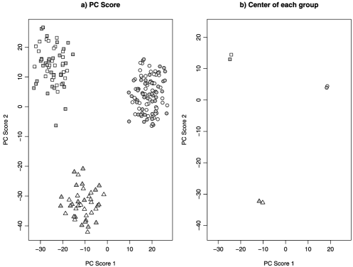
Figure 2: Shrinkage-adjusted PC scores of the data in Figure 1. Different symbols represent different groups. White background color represents the training set and grey background color represents the test set. (a) Plots of all simulation samples. (b) Center of each group.

the predicted PC scores of the test data are comparable to those of the training data. This indicates that our method is effective in correcting for the shrinkage bias.

Next, we conducted a new simulation to check the accuracy of our estimators. For the $j$th sample ($j=1,\ldots,n$), its $i$th variable was generated as

$$x_{ij}=\cases{\lambda_{1}z_{ij},&\quad$i=1$,\cr\lambda_{2}z_{ij},&\quad$i=2$,\cr z_{ij},&\quad$i>2$,}$$

where $\lambda_{1}>\lambda_{2}>1$ and $z_{ij}\sim N(0,2^{2})$. Under this setting, $\lambda_{1}$ and $\lambda_{2}$ are the first and the second population eigenvalues. The first and second population eigenvectors are $e_{1}=\{1,0,\ldots,0\}$ and $e_{2}=\{0,1,0,\ldots,0\}$, respectively. We set the standard deviation of $z_{ij}$ to 2 instead of 1, which allows us to test whether the rescaling procedure works properly. We tried different values of $\gamma$ and $n$, but set $\lambda_{1}$ and $\lambda_{2}$ to $4(1+\sqrt{\gamma})$ and $2(1+\sqrt{\gamma})$, respectively.

We split the simulated samples into test and training sets, each with $n$ samples. We first estimated the asymptotic shrinkage factor based on the training samples. We then calculated the predicted PC scores on the test samples. To assess the accuracy of shrinkage factor estimator for each PC, we empirically estimated the shrinkage factor by the ratio of the mean predicted PC scores of the test samples to the mean PC scores of the training samples. That is, for the $v$th PC, the empirical shrinkage factor is estimated by $\sqrt{\sum_{i=1}^{n}q_{vi}^{2}/\sum_{k=1}^{n}p_{vk}^{2}}$. On the training samples, we also estimated the empirical angle between the sample and (known) population eigenvectors, as well as the empirical angle between PC scores from sample and population eigenvectors. The asymptotic theoretical estimates were also calculated. Tables 1 and 2 summarize the simulation results. Our asymptotic estimators provide accurate estimates for the angles and the shrinkage factor.

Table 1: Cosine angle estimates of eigenvectors and PC scores based on 1000 simulations. “Angle” indicates the theoretical asymptotic $\cos(\mathrm{angle})$, “Estimate1” indicates the empirical $\cos(\mathrm{angle})$ estimator, “Estimate2” indicates the asymptotic $\cos(\mathrm{angle})$ estimator. For each estimator, each entry represents mean of $1000$ simulation results with standard error in parentheses

		PC 1			PC 2
			Angle	Angle		Angle	Angle
$\bolds\gamma$	$\bolds n$	Angle	Estimate1	Estimate2	Angle	Estimate1	Estimate2
Eigenvectors
$1$	$100$	$0.93$	$0.93\ (0.013)$	$0.91\ (0.027)$	$0.82$	$0.81\ (0.053)$	$0.80\ (0.052)$
	$200$		$0.93\ (0.009)$	$0.92\ (0.014)$		$0.81\ (0.030)$	$0.81\ (0.032)$
$20$	$100$	$0.70$	$0.69\ (0.037)$	$0.70\ (0.031)$	$0.51$	$0.50\ (0.053)$	$0.50\ (0.058)$
	$200$		$0.69\ (0.023)$	$0.70\ (0.022)$		$0.51\ (0.036)$	$0.51\ (0.041)$
$100$	$100$	$0.53$	$0.53\ (0.034)$	$0.53\ (0.031)$	$0.37$	$0.35\ (0.043)$	$0.35\ (0.047)$
	$200$		$0.53\ (0.024)$	$0.53\ (0.024)$		$0.36\ (0.029)$	$0.36\ (0.033)$
$500$	$100$	$0.38$	$0.38\ (0.029)$	$0.38\ (0.028)$	$0.25$	$0.24\ (0.033)$	$0.24\ (0.037)$
	$200$		$0.38\ (0.020)$	$0.38\ (0.020)$		$0.25\ (0.021)$	$0.25\ (0.024)$
PC scores
$1$	$100$	$0.99$	$0.99\ (0.004)$	$0.98\ (0.016)$	$0.94$	$0.93\ (0.036)$	$0.91\ (0.048)$
	$200$		$0.99\ (0.003)$	$0.99\ (0.006)$		$0.94\ (0.019)$	$0.93\ (0.024)$
$20$	$100$	$0.98$	$0.97\ (0.083)$	$0.98\ (0.008)$	$0.89$	$0.86\ (0.105)$	$0.87\ (0.055)$
	$200$		$0.97\ (0.055)$	$0.98\ (0.005)$		$0.88\ (0.073)$	$0.88\ (0.036)$
$100$	$100$	$0.97$	$0.97\ (0.079)$	$0.97\ (0.009)$	$0.88$	$0.85\ (0.109)$	$0.86\ (0.060)$
	$200$		$0.97\ (0.058)$	$0.97\ (0.006)$		$0.86\ (0.076)$	$0.87\ (0.039)$
$500$	$100$	$0.97$	$0.96\ (0.084)$	$0.97\ (0.010)$	$0.87$	$0.83\ (0.117)$	$0.84\ (0.069)$
	$200$		$0.96\ (0.058)$	$0.97\ (0.007)$		$0.86\ (0.076)$	$0.86\ (0.038)$

Table 2: Shrinkage factor estimates based on 1000 simulation. “Factor” indicates the theoretical asymptotic factor, “Estimate1” indicates the empirical shrinkage factor estimator, “Estimate2” indicates the asymptotic shrinkage factor estimator. For each estimator, each entry represents mean of $1000$ simulation results with standard error in parentheses

		PC 1			PC 2
			Factor	Factor		Factor	Factor
$\bolds\gamma$	$\bolds n$	Factor	Estimate1	Estimate2	Factor	Estimate1	Estimate2
00$1$	$100$	0.88	$0.88\ (0.017)$	$0.87\ (0.076)$	0.75	$0.75\ (0.044)$	$0.76\ (0.063)$
	$200$		$0.88\ (0.013)$	$0.87\ (0.054)$		$0.75\ (0.027)$	$0.75\ (0.044)$
$20$	$100$	$0.51$	$0.51\ (0.037)$	$0.51\ (0.038)$	$0.33$	$0.34\ (0.033)$	$0.32\ (0.038)$
	$200$		$0.51\ (0.025)$	$0.51\ (0.026)$		$0.34\ (0.022)$	$0.33\ (0.028)$
$100$	$100$	$0.30$	$0.30\ (0.024)$	$0.30\ (0.030)$	$0.17$	$0.17\ (0.019)$	$0.17\ (0.023)$
	$200$		$0.30\ (0.017)$	$0.30\ (0.023)$		$0.18\ (0.013)$	$0.17\ (0.017)$
$500$	$100$	$0.16$	$0.15\ (0.014)$	$0.16\ (0.020)$	$0.08$	$0.08\ (0.010)$	$0.08\ (0.013)$
	$200$		$0.15\ (0.010)$	$0.16\ (0.014)$		$0.08\ (0.007)$	$0.08\ (0.009)$

Finally, we conducted simulation to demonstrate an application of the bias-adjusted PC scores in PC regression. PC regression has been widely used in microarray gene-expression studies bovelstad2007 . In this simulation, we let $p=5000$, and our set up is very similar to the first simulation of Bair et al. bair2006prediction . Let $x_{ij}$ denote the gene expression level of the $i$th gene for the $j$th subject. We generated each $x_{ij}$ according to

$$x_{ij}=\cases{3+\varepsilon,&\quad$i\leq g,j\leq n/2$,\cr 4+\varepsilon,&\quad$i\leq g,j>n/2$,\cr 3.5+\varepsilon,&\quad$i>g$,}$$

and the outcome variable $y_{j}$ as

$$y_{j}=\frac{2}{g}\sum_{i=1}^{g}x_{ij}+\varepsilon_{y},$$

where $n$ is the number of samples, $g$ is the number of genes that are differentially expressed and associated with the phenotype, $\varepsilon\sim N(0,2^{2})$ and $\varepsilon_{y}\sim N(0,1)$. A total of eight different combinations of $n$ and $g$ were simulated. For the training data, we fit the PC regression with the first PC as the covariate and computed the mean square error (MSE). For the test samples with the same configuration of the training samples, we applied the PC model built on the training data to predict the phenotypes using the unadjusted and adjusted PC scores. The results are presented in Table 3. We see that the MSE of the test

Table 3: Mean Square Error (MSE) of the PC regression based on gene-expression microarray data simulation with and without shrinkage adjustment. 1000 simulation were conducted. Each entry in the table represents mean of the MSE with standard error in parentheses

		Test data	Test data
$\bolds n$	$\bolds g$	without adjustment	with adjustment	Training data
$100$	$150$	$1.97\ (0.256)$	$1.70\ (0.284)$	$1.61\ (0.284)$
$100$	$300$	$1.63\ (0.230)$	$1.17\ (0.167)$	$1.12\ (0.158)$
$100$	$500$	$1.43\ (0.204)$	$1.07\ (0.157)$	$1.03\ (0.147)$
$100$	$1000$	$1.22\ (0.182)$	$1.03\ (0.148)$	$0.99\ (0.142)$
$200$	$150$	$1.73\ (0.159)$	$1.33\ (0.133)$	$1.30\ (0.131)$
$200$	$300$	$1.39\ (0.139)$	$1.08\ (0.105)$	$1.07\ (0.110)$
$200$	$500$	$1.24\ (0.131)$	$1.04\ (0.105)$	$1.01\ (0.101)$
$200$	$1000$	$1.10\ (0.114)$	$1.02\ (0.101)$	$1.00\ (0.101)$

set without bias adjustment is appreciably higher than that of the test set with bias adjustment, and the MSE of the test set with bias adjustment is comparable with the MSE of the training set.

4 Real data example

Here, we demonstrate that the shrinkage phenomenon appears in real data, and can be adjusted by our method. For this purpose, genetic data on samples from unrelated individuals in the Phase 3 HapMap study (http://hapmap.ncbi.nlm.nih.gov/) were used. HapMap is a dense genotyping study designed to elucidate population genetic differences. The genetic data are discrete, assuming the values 0, 1 or 2 at each genomic marker (also known as SNPs) for each individual. Data from CEU individuals (of northern and western European ancestry) were compared with data from TSI individuals (Toscani individuals from Italy, representing southern European ancestry).

Figure 3: Scree plot of the first 30 sample eigenvalues, CEU${}+{}$TSI dataset.

Some initial data trimming steps are standard in genetic analysis. We first removed apparently related samples, and removed genomic markers with more than a 10% missing rate, and those with frequency less than 0.01 for the minor genetic allele. To avoid spurious PC results, we further pruned out SNPs that are in high linkage disequlibrium (LD) fellay2007 . Lastly, we excluded $7$ samples with PC scores greater than 6 standard deviations away from the mean of at least one of the top significant PCs [i.e., with Tracy–Widom (TW) Test $p$-value $<$0.01] price2006pca , patterson2006psa . The final dataset contained 178 samples (101 CEU, 77 TSI) and 100,183 markers. We mean-centered and variance-standardized the genotypes for each marker price2006pca . The screeplot of the sample eigenvalues is presented in Figure 3. The first eigenvalue is substantially larger than the rest of the eigenvalues, although the TW test actually identifies two significant PCs. Figure 3 suggests that our data approximately satisfies the spiked eigenvalue assumption.

We estimated the asymptotic shrinkage factor and compared it with the following jackknife-based shrinkage factor estimate. For the first PC, we first computed the scores of all samples. Next, we removed one sample at a time and computed the (unadjusted) predicted PC score. We then calculated the jackknife estimate as the square root of the ratio of the means of the sample PC score and the predicted PC score. The jackknife shrinkage factor estimate is $0.319$, which is close to our asymptotic estimate $0.325$. Figure 4 shows the PC scores from the

Figure 4: An instance with and without shrinkage adjustment, performed on Hapmap CEU(*) and TSI($+$). “*” and “$+$” represent PC scores using all data. The $161$st sample was excluded from PCA, and PC score for it was predicted. The grey rectangle represents the predicted PC score without shrinkage adjustment and the grey circle represents the predicted PC score after the shrinkage adjustment.

whole sample, the predicted PC score of an illustrative excluded sample, and its bias-adjusted predicted score. Clearly, the predicted PC score without adjustment is very biased toward zero, while the bias-adjusted PC score is not.

5 Discussion and conclusions

In this paper, we have identified and explored the shrinkage phenomenon of the predicted PC scores, and have developed a novel method to adjust these quantities. We also have constructed the asymptotic estimator of correlation coefficient between PC scores from population eigenvectors and sample eigenvectors. In simulation experiments and real data analysis, we have demonstrated the accuracy of our estimates, and the capability to increase prediction accuracy in PC regression by adopting shrinkage bias adjustment. For achieving these, we consider asymptotics in the large $p$, large $n$ framework, under the spiked population model.

We believe that this asymptotic regime applies well to many high-dimensional datasets. It is not, however, the only model paradigm applied to such data. For example, the large $p$ small $n$ paradigm hall2005geometric , ahn2007high , which assumes $p/n\rightarrow\infty$, has also been explored. Under this assumption, Jung and Marron sungkyu have shown that the consistency and the strong inconsistency of the sample eigenvectors to population eigenvectors depend on whether $p$ increases at a slower or faster rate than $\lambda_{v}$. It may be argued that for real data where $p/n$ is “large,” we should follow the paradigm of Hall, Marron and Neeman hall2005geometric , Ahn et al. ahn2007high . However, for any real study, it is unclear how to test whether $p$ increases at a faster rate than $\lambda_{v}$, or vice versa, making the application of Hall, Marron and Neeman hall2005geometric , Ahn et al. ahn2007high difficult in practice. Furthermore, the scenario where $p$ and $\lambda_{v}$ grow at the same rate is scientifically more interesting, for which we are aware of no theoretical results. In contrast, our asymptotic results can be straightforwardly applied. Further, our simulation results indicate that for $p/n$ as large as 500, our asymptotic results still hold well. We believe that the approach we describe here applies to many datasets.

Although the results from the spiked model are useful, it is likely that observed data has more structure than allowed by the model. Recently, several methods have been suggested to estimate population eigenvalues under more general scenarios elkaroui2008sel , rao2008 . However, no analogous results are available for the eigenvectors. In data analysis, jackknife estimators, as demonstrated in the real data analysis section, can be used. However, resampling approaches are very computationally intensive, and it remains of interest to establish the asymptotic behavior of eigenvectors in a variety of situations.

We note that inconsistency of the sample eigenvectors does not necessarily imply poor performance of PCA. For example, PCA has been successfully applied in genome-wide association studies for accurate estimation of ethnicity price2006pca , and in PC regression for microarrays ma2006additive . However, for any individual study we cannot rule out the possibility of poor performance of the PC analysis. Our asymptotic result on the correlation coefficient between PC scores from sample and population eigenvectors provides us a measure to quantify the performance of PC analysis.

For the CEU/TSI data, SNP pruning was applied to adjust for strong LD among adjacent SNPs. Such SNP pruning is a common practice in the analysis of GWAS data, and has been implemented in the popular GWAS analysis software Plink purcell2007pts . The primary goal of SNP pruning is to avoid spurious PC results unrelated to population substructures. Technically, our approach does not rely on any independence assumption of the SNPs. However, strong local correlation may affect eigenvalues considerably. Thus, the value in SNP pruning may be viewed as helping the data better accord with the assumptions of the spiked population model. From the CEU/TSI data and our experience in other GWAS data, we have found that the most common pruning procedure implemented in Plink is sufficient for us to then apply our methods.

6 Proofs

Note that $\mathbf{E}\bolds{\Lambda}^{1/2}\mathbf{Z}\mathbf{Z}^{T}\bolds{\Lambda}^{1/2}\mathbf{E}^{T}$ and $\bolds{\Lambda}^{1/2}\mathbf{Z}\mathbf{Z}^{T}\bolds{\Lambda}^{1/2}$ have the same eigenvalues, and $\mathbf{E}^{T}\mathbf{U}$ is the eigenvector matrix of $\bolds{\Lambda}^{1/2}\mathbf{Z}\mathbf{Z}^{T}\bolds{\Lambda}^{1/2}$. Since eigenvalues and angles between sample and population eigenvectors are what we concerned about, without loss of generality (WLOG), in the sequel, we assume $\bolds{\Lambda}$ to be the population covariance matrix.

6.1 Notation

We largely follow notation in Paul paul2007 . We denote $\lambda_{v}(\mathbf{S})$ as the $v$th largest eigenvalue of $\mathbf{S}$. Let suffice $A$ represent the first $m$ coordinates and $B$ represent the remaining coordinates. Then we can partition $\mathbf{S}$ into

$$\mathbf{S}=\left[\matrix{\mathbf{S}_{AA}&\mathbf{S}_{AB}\cr\mathbf{S}_{BA}&\mathbf{S}_{BB}}\right].$$

We similarly partition the $v$th eigenvector $\mathbf{u}_{v}^{T}$ into $(\mathbf{u}_{A,v},\mathbf{u}_{B,v})$ and $\mathbf{Z}^{T}$ into $[\mathbf{Z}_{A}^{T},\mathbf{Z}_{B}^{T}]$. Define $R_{v}$ as $\|\mathbf{u}_{B,v}\|$ and let $\mathbf{a}_{v}=\mathbf{u}_{A,v}/\sqrt{1-R_{v}^{2}}$, then we get $\|\mathbf{a}_{v}\|=1$.

Applying singular value decomposition (SVD) to $\mathbf{Z}_{B}/\sqrt{n}$, we get

$$\frac{1}{\sqrt{n}}\mathbf{Z}_{B}=\mathbf{V}\mathbf{M}^{1/2}\mathbf{H}^{T},$$ (9)

where $\mathbf{M}=\operatorname{diag}(\mu_{1},\ldots,\mu_{p-m})$ is a $(p-m)\times(p-m)$ diagonal matrix of ordered eigenvalues of $\mathbf{S}_{BB}$, $\mathbf{V}$ is a $(p-m)\times(p-m)$ orthogonal matrix and $\mathbf{H}$ is an $n\times(p-m)$ matrix. For $n\geq p-m$, $\mathbf{H}$ has full rank orthogonal columns. When $n<p-m$, $\mathbf{H}$ has more columns than rows, hence it does not have full rank orthogonal columns. For the later case, we make $\mathbf{H}=[\mathbf{H}_{n},0]$ where $\mathbf{H}_{n}$ is an $n\times n$ orthogonal matrix.

6.2 Propositions

We introduce two propositions for later use. The proofs of the two propositions can be found in Sections 6.5 and 6.6.

Proposition 1.

Suppose $\mathbf{Y}$ is an $n\times m$ matrix with fixed $m$ and each entry of $\mathbf{Y}$ is i.i.d. random variable which satisfies the moment condition of $z_{ij}$ in Assumption 1. Let $\mathbf{C}$ be an $n\times n$ symmetric nonnegative definite random matrix and independent of $\mathbf{Y}$. Further, assume $\|\mathbf{C}\|=O(1)$. Then

$$\frac{1}{n}\mathbf{Y}^{T}\mathbf{C}\mathbf{Y}-\frac{1}{n}\operatorname{trace}(\mathbf{C})\mathbf{I}\stackrel{{\scriptstyle p}}{{\rightarrow}}0$$

as $n\rightarrow\infty$.

Proposition 2.

Suppose $\mathbf{y}$ is an $n$-dimensional random vector which follows the same distribution of the row vectors of $\mathbf{Y}$ and independent of $\mathbf{S}_{BB}$. Let $f(x)$ be a bounded continuous function on $[(1-\sqrt{\gamma})^{2},(1+\sqrt{\gamma})^{2}]$ and $f(0)=0$. Suppose $\mathbf{F}=\mathrm{diag}(f(\mu_{1}),\ldots,f(\mu_{p-m}))$, where $\{\mu_{i}\}_{i=1}^{p-m}$ are ordered eigenvalues of $\mathbf{M}$ which is defined on (9), then

$$\frac{1}{n}\mathbf{y}^{T}\mathbf{H}\mathbf{F}\mathbf{H}^{T}\mathbf{y}-\gamma\int{f(x)\,dF_{\gamma}(x)}\stackrel{{\scriptstyle p}}{{\rightarrow}}0$$

as $n\rightarrow\infty$, where $F_{\gamma}(x)$ is a distribution function of Marčenko–Pastur law with parameter $\gamma$ marvcenko1967 .

6.3 Proof of part (i) of Lemma 1

6.3.1 When $p$ is fixed

By the strong law of large numbers, $\mathbf{S}\stackrel{{\scriptstyle\mathrm{a.s.}}}{{\rightarrow}}\bolds{\Lambda}$. Since eigenvalues are continuous with respect to the operator norm, the lemma follows after applying continuous mapping theorem.

6.3.2 When $p\rightarrow\infty$

For every small $\varepsilon>0$, there exist $\tilde{p}(n)$ and $\gamma_{\varepsilon}$ such that $\tilde{p}(n)/n\rightarrow\gamma_{\varepsilon}>0$, $\lambda_{v}(1+\gamma_{\varepsilon}/(\lambda_{v}-1))<\lambda_{v}+\varepsilon$ for all $v\leq m$, $(1+\sqrt{\gamma_{\varepsilon}})^{2}<1+\varepsilon$ and $(1-\sqrt{\gamma_{\varepsilon}})^{2}>1-\varepsilon$. For simplicity, we denote $\tilde{p}(n)$ as $\tilde{p}$. Suppose $\mathbf{Z}_{\tilde{p}}$ is a $\tilde{p}\times n$ matrix that satisfies the moment condition of $z_{ij}$ in Assumption 1. Define an augmented data matrix $\tilde{\mathbf{X}}^{T}=[\mathbf{Z}^{T}\bolds{\Lambda},\mathbf{Z}_{\tilde{p}}^{T}]^{T}$ and its sample covariance matrix $\tilde{\mathbf{S}}=\tilde{\mathbf{X}}\tilde{\mathbf{X}}^{T}$. Let $\mathbf{S}$ be a $p\times p$ upper left submatrix of $\tilde{\mathbf{S}}$. We also let $\hat{\mathbf{S}}$ be an $(m+1)\times(m+1)$ upper left submatrix of $\tilde{\mathbf{S}}$. For $v\leq(m+1)$, by the interlacing inequality (Theorem 4.3.15 of Horn and Johnson horn1990matrix ),

$$\lambda_{v}(\hat{\mathbf{S}})\leq\lambda_{v}(\mathbf{S})\leq\lambda_{v}(\tilde{\mathbf{S}}).$$

Since $\lambda_{v}(\hat{\mathbf{S}})\stackrel{{\scriptstyle\mathrm{a.s.}}}{{\rightarrow}}\lambda_{v}$, $\lambda_{v}(\tilde{\mathbf{S}})\stackrel{{\scriptstyle\mathrm{a.s.}}}{{\rightarrow}}\lambda_{v}(1+\gamma_{\varepsilon}/(\lambda_{v}-1))<1+\varepsilon$ for $v\leq m$, and $\lambda_{v}(\tilde{\mathbf{S}})\stackrel{{\scriptstyle\mathrm{a.s.}}}{{\rightarrow}}(1+\sqrt{\gamma_{\varepsilon}})^{2}<1+\varepsilon$ for $v=m+1$, we have

$$\lambda_{v}-o(1)\leq\lambda_{v}(\mathbf{S})<\lambda_{v}+\varepsilon+o(1)\qquad\mbox{for }v\leq m+1.$$

Thus,

$$\lambda_{v}(\mathbf{S})\stackrel{{\scriptstyle\mathrm{a.s.}}}{{\rightarrow}}\lambda_{v}\qquad\mbox{for }v\leq m+1.$$ (10)

Similarly by the interlacing inequality, we get

$$\lambda_{\tilde{p}}(\tilde{S})\leq\lambda_{p}(S)\leq\lambda_{m+1}(S).$$

Since $\lambda_{m+1}(S)\stackrel{{\scriptstyle\mathrm{a.s.}}}{{\rightarrow}}1$ and $\lambda_{\tilde{p}}(\tilde{S})\stackrel{{\scriptstyle\mathrm{a.s.}}}{{\rightarrow}}(1-\sqrt{\gamma_{\varepsilon}})^{2}>1-\varepsilon$, we conclude that

$$\lambda_{p}(S)\stackrel{{\scriptstyle\mathrm{a.s.}}}{{\rightarrow}}1.$$ (11)

Part (i) of Lemma 1 follows by (10) and (11).

6.4 Proof of part (ii) of Lemma 2

Our proof of Lemma 2(ii) closely follows the arguments in Paul paul2007 . From paul2007 , it can be shown that

$$\biggl{(}\mathbf{S}_{AA}+\frac{1}{n}\bolds{\Lambda}_{A}^{1/2}\mathbf{Z}_{A}\mathbf{H}\mathbf{M}(d_{v}\mathbf{I}-\mathbf{M})^{-1}\mathbf{H}^{T}\mathbf{Z}_{A}^{T}\bolds{\Lambda}_{A}^{1/2}\biggr{)}\mathbf{a}_{v}=d_{v}\mathbf{a}_{v}$$ (12)

and

$$\mathbf{a}_{v}^{T}\biggl{(}\mathbf{I}+\frac{1}{n}\bolds{\Lambda}_{A}^{1/2}\mathbf{Z}_{A}\mathbf{H}\mathbf{M}(d_{v}\mathbf{I}-\mathbf{M})^{-2}\mathbf{H}^{T}\mathbf{Z}_{A}^{T}\bolds{\Lambda}_{A}^{1/2}\biggr{)}\mathbf{a}_{v}=\frac{1}{1-R_{v}^{2}},$$ (13)

where $\bolds{\Lambda}_{A}=\mathrm{diag}\{\lambda_{1},\ldots,\lambda_{m}\}$.

6.4.1 When $\lambda_{v}>1+\sqrt{\gamma}$

We can show that

$$\langle\mathbf{a}_{v},\mathbf{e}_{A,v}\rangle\stackrel{{\scriptstyle p}}{{\rightarrow}}1$$ (14)

and

$$\frac{1}{n}\mathbf{z}_{Av}^{T}\mathbf{H}\mathbf{M}(d_{v}\mathbf{I}-\mathbf{M})^{-2}\mathbf{H}^{T}\mathbf{z}_{Av}\stackrel{{\scriptstyle p}}{{\rightarrow}}\cases{\displaystyle\gamma\int{\frac{x}{(\rho_{v}-x)^{2}}\,dF_{\gamma}(x)},&\quad for $\gamma>0$,\vspace*{2pt}\cr 0,&\quad for $\gamma=0$,}$$ (15)

where $\mathbf{e}_{A,v}$ is a vector of the first $m$ coordinates of the $v$th population eigenvector $\mathbf{e}_{v}$, $\rho_{v}$ is $\lambda_{v}(1+\frac{\gamma}{\lambda_{v}-1})$ and $\mathbf{z}_{Av}$ is a vector of $v$th row of $\mathbf{Z}_{A}$. The proofs can be found in Section 6.4.3. Note that $\mathbf{e}_{v}$ is a vector with $1$ in its $v$th coordinate and $0$ elsewhere. WLOG, we assume that $\langle\mathbf{e}_{v},\mathbf{u}_{v}\rangle\geq 0$. Since $\langle\mathbf{e}_{v},\mathbf{u}_{v}\rangle=\sqrt{1-R_{v}^{2}}\langle\mathbf{e}_{A,v},\mathbf{a}_{v}\rangle$, $\langle\mathbf{e}_{v},\mathbf{u}_{v}\rangle\stackrel{{\scriptstyle p}}{{\rightarrow}}\sqrt{1-R_{v}^{2}}$. By (13) and (15), we can show that

$$\frac{1}{1-R_{v}^{2}}\stackrel{{\scriptstyle p}}{{\rightarrow}}\cases{\displaystyle 1+\lambda_{v}\gamma\int{\frac{x}{(\rho_{v}-x)^{2}}\,dF_{\gamma}(x)},&\quad for $\gamma>0$,\vspace*{2pt}\cr 1,&\quad for $\gamma=0$.}$$ (16)

From Lemma B.2 of paul2007 ,

$$\int{\frac{x}{(\rho_{v}-x)^{2}}\,dF_{\gamma}(x)}=\frac{1}{(\lambda_{v}-1)^{2}-\gamma}.$$ (17)

Thus,

$$\sqrt{1-R_{v}^{2}}\stackrel{{\scriptstyle p}}{{\rightarrow}}\cases{\displaystyle\sqrt{\biggl{(}1-\frac{\gamma}{(\lambda_{v}-1)^{2}}\biggr{)}\Big{/}\biggl{(}1+\frac{\gamma}{\lambda_{v}-1}\biggr{)}},&\quad for $\gamma>0$,\vspace*{2pt}\cr 1,&\quad for $\gamma=0$.}$$ (18)

It concludes the proof of the first part of Lemma 2(ii).

6.4.2 When $1<\lambda_{v}\leq 1+\sqrt{\gamma}$

Here, we only need to consider $\gamma>0$ because no eigenvalue satisfies this condition when $\gamma=0$. We first show that $R_{v}\stackrel{{\scriptstyle p}}{{\rightarrow}}1$, which implies $\mathbf{u}_{A,v}\stackrel{{\scriptstyle p}}{{\rightarrow}}0$, hence $\langle\mathbf{e}_{v},\mathbf{u}_{v}\rangle\stackrel{{\scriptstyle p}}{{\rightarrow}}0$. For any $\varepsilon>0$ and $x\geq 0$, define

$$(x)_{\varepsilon}=\cases{x,&\quad if $x>\varepsilon$,\cr\varepsilon,&\quad if $x\leq\varepsilon$,}$$

and

$$\mathbf{G}_{\varepsilon}=\mathrm{diag}\bigl{(}d_{v}/\bigl{(}(d_{v}-\mu_{1})^{2}\bigr{)}_{\varepsilon},\ldots,d_{v}/\bigl{(}(d_{v}-\mu_{p-m})^{2}\bigr{)}_{\varepsilon}\bigr{)},$$

then by Propositions 1 and 2,

$$\frac{1}{n}\mathbf{z}_{Av}^{T}\mathbf{H}\mathbf{G}_{\varepsilon}\mathbf{H}^{T}\mathbf{z}_{Av}\stackrel{{\scriptstyle p}}{{\rightarrow}}\gamma\int{\frac{x}{((\rho_{v}-x)^{2})_{\varepsilon}}\,dF_{\gamma}(x)}.$$ (19)

By monotone convergence theorem,

$$\gamma\int{\frac{x}{((\rho_{v}-x)^{2})_{\varepsilon}}\,dF_{\gamma}(x)}\stackrel{{\scriptstyle\varepsilon\rightarrow 0}}{{\longrightarrow}}\gamma\int{\frac{x}{(\rho_{v}-x)^{2}}\,dF_{\gamma}(x)}.$$ (20)

The right-hand side of (20) is

$$\int_{a}^{b}{\frac{\sqrt{(b-x)(x-a)}}{2\pi(\rho_{v}-x)^{2}}\,dx},$$ (21)

where $a=(1-\sqrt{\gamma})^{2}$ and $b=(1+\sqrt{\gamma})^{2}$. Since (21) equals $\infty$ for any $a\leq\rho_{v}\leq b$, we conclude that

$$\frac{1}{n}\mathbf{z}_{Av}^{T}\mathbf{H}\mathbf{M}(d_{v}\mathbf{I}-\mathbf{M})^{-2}\mathbf{H}^{T}\mathbf{z}_{Av}\stackrel{{\scriptstyle p}}{{\rightarrow}}\infty.$$ (22)

Therefore $R_{v}\stackrel{{\scriptstyle p}}{{\rightarrow}}1$, which proves the second part of Lemma 2(ii).

6.4.3 Proof of (14) and (15)

Define

$$\mathcal{R}_{v} = \sum_{k\neq v}^{m}\frac{\lambda_{v}}{\rho_{v}(\lambda_{k}-\lambda_{v})}\mathbf{e}_{A,k}\mathbf{e}_{A,k}^{T},$$

$$\mathcal{D}_{v} = \mathbf{S}_{AA}+\mathbf{S}_{AB}(d_{v}\mathbf{I}-\mathbf{S}_{BB})^{-1}\mathbf{S}_{BA}-(\rho_{v}/\lambda_{v})\bolds{\Lambda}_{A},$$

$$\alpha_{v} = \|\mathcal{R}_{v}\mathcal{D}_{v}\|+|d_{v}-\rho_{v}|\|\mathcal{R}_{v}\|\quad\mbox{and}\quad\beta_{v}=\|\mathcal{R}_{v}\mathcal{D}_{v}\mathbf{e}_{A,v}\|.$$

With the exactly same argument of paul2007 , it can be shown that

$$\mathbf{a}_{v}-\mathbf{e}_{A,v}=-\mathcal{R}_{v}\mathcal{D}_{v}\mathbf{e}_{A,v}+\mathbf{r}_{v},$$

where $\mathbf{r}_{v}=-(1-\langle\mathbf{e}_{A,v},\mathbf{a}_{v}\rangle)\mathbf{e}_{A,v}-\mathcal{R}_{v}\mathcal{D}_{v}(\mathbf{a}_{v}-\mathbf{e}_{A,v})+(d_{v}-\rho_{v})\mathcal{R}_{v}(\mathbf{a}_{v}-\mathbf{e}_{A,v})$. By Lemma 1 of paul2005 , $r_{v}=o_{p}(1)$, if $\alpha_{v}=o_{p}(1)$ and $\beta_{v}=o_{p}(1)$.

When $\gamma=0$, $\mathbf{S}_{AA}-(\rho_{v}/\lambda_{v})\bolds{\Lambda}_{A}\stackrel{{\scriptstyle p}}{{\rightarrow}}0$ and the remainder of $\mathcal{D}_{v}$ is

$$\quad\mathbf{S}_{AB}(d_{v}\mathbf{I}-\mathbf{S}_{BB})^{-1}\mathbf{S}_{BA}=\frac{1}{n}\bolds{\Lambda}_{A}^{1/2}\mathbf{Z}_{A}\mathbf{H}\mathbf{M}(d_{v}\mathbf{I}-\mathbf{M})^{-1}\mathbf{H}^{T}\mathbf{Z}_{A}^{T}\bolds{\Lambda}_{A}^{1/2}.$$ (23)

Since $d_{v}\stackrel{{\scriptstyle\mathrm{a.s.}}}{{\rightarrow}}\lambda_{v}$ and $\mu_{1}\stackrel{{\scriptstyle\mathrm{a.s.}}}{{\rightarrow}}1$,

$$\|\mathbf{H}\mathbf{M}(d_{v}\mathbf{I}-\mathbf{M})^{-1}\mathbf{H}^{T}\|\stackrel{{\scriptstyle\mathrm{a.s.}}}{{\rightarrow}}1/(\lambda_{v}-1).$$

By Proposition 1,

$$0\leq\|(\ref{PF13_1})\|\leq\lambda_{1}\frac{p\mu_{1}}{n(d_{v}-\mu_{1})}+o_{p}(1)=o_{p}(1),$$ (24)

hence $\mathcal{D}_{v}=o_{p}(1)$.

When $\gamma>0$, $\mathcal{D}_{v}$ can be written as

$$\hskip 28.0pt\mathcal{D}_{v} = [\mathbf{S}_{AA}-\bolds{\Lambda}_{A}]$$

$${}+\biggl{[}\bolds{\Lambda}_{A}^{1/2}\biggl{(}\frac{1}{n}\mathbf{Z}_{A}\mathbf{H}\mathbf{M}(\rho_{v}\mathbf{I}-\mathbf{M})^{-1}\mathbf{H}^{T}\mathbf{Z}_{A}$$

$$\hskip 49.0pt{}-\frac{1}{n}\operatorname{trace}\bigl{(}\mathbf{M}(\rho_{v}\mathbf{I}-\mathbf{M})^{-1}\bigr{)}\mathbf{I}\biggr{)}\bolds{\Lambda}_{A}^{1/2}\biggr{]}$$

$${}+\biggl{[}\biggl{(}\frac{1}{n}\operatorname{trace}\bigl{(}\mathbf{M}(\rho_{v}\mathbf{I}-\mathbf{M})^{-1}\bigr{)}-\gamma\int{\frac{x}{\rho_{v}-x}\,dF_{\gamma}(x)}\biggr{)}\bolds{\Lambda}_{A}\biggr{]}$$

$${}+\biggl{[}(\rho_{v}-d_{v})\frac{1}{n}\bolds{\Lambda}_{A}^{1/2}\mathbf{Z}_{A}\mathbf{H}\mathbf{M}(\rho_{v}\mathbf{I}-\mathbf{M})^{-1}(d_{v}\mathbf{I}-\mathbf{M})^{-1}\mathbf{H}^{T}\mathbf{Z}_{A}\bolds{\Lambda}_{A}^{1/2}\biggr{]}.$$

The first term of the right-hand side is $o_{p}(1)$ by the weak law of large number. The second and third terms are $o_{p}(1)$ by Propositions 1 and 2. For the fourth term, $\rho_{v}-d_{v}=o_{p}(1)$ and its remainder part is $O_{p}(1)$. Therefore, $\mathcal{D}_{v}=o_{p}(1)$. By combining the above results and $\mathcal{R}_{v}=O_{p}(1)$ plus $d_{v}-\rho_{v}=o_{p}(1)$, we prove (14).

For (15): When $\gamma=0$, (15) can be proved by the exactly same way used to show (24). When $\gamma>0$, $d_{v}\stackrel{{\scriptstyle\mathrm{a.s.}}}{{\rightarrow}}\rho_{v}$, and $\mu_{1}\stackrel{{\scriptstyle\mathrm{a.s.}}}{{\rightarrow}}(1+\sqrt{\gamma})^{2}<\rho_{v}$, hence $\|\mathbf{C}\|\stackrel{{\scriptstyle\mathrm{a.s.}}}{{\rightarrow}}\frac{(1+\sqrt{\gamma})^{2}}{(\rho_{v}-(1+\sqrt{\gamma})^{2})^{2}}$. Therefore, the result follows according to Propositions 1 and 2.

6.5 Proof of Proposition 1

Let $\mu_{1}\geq\mu_{2}\geq\cdots\geq\mu_{n}$ be the ordered eigenvalues of $\mathbf{C}$, and $c_{ij}$ be the $(i,j)$th element of $\mathbf{C}$. Suppose $\mathbf{y}_{s}$ is the $s$th column of $\mathbf{Y}$, and $y_{ij}$ is the $(i,j)$th element of $\mathbf{Y}$. We further define $\psi(s,s)=\frac{1}{n}\mathbf{y}_{s}^{T}\mathbf{C}\mathbf{y}_{s}-\frac{1}{n}\operatorname{trace}(\mathbf{C})$ and $\psi(s,t)=\frac{1}{n}\mathbf{y}_{s}^{T}\mathbf{C}\mathbf{y}_{t}$ for $s\neq t$. The conditional mean of $\psi(s,s)$ given $\mathbf{C}$ is

$$E(\psi(s,s)|\mathbf{C}) = E\biggl{(}\frac{1}{n}\sum_{i,j}c_{ij}y_{is}y_{js}|\mathbf{C}\biggr{)}-\frac{1}{n}\sum_{i=1}^{n}\mu_{i}$$

$$= \frac{1}{n}\sum_{i=1}^{n}c_{ii}E(y_{is}^{2})+\frac{2}{n}\sum_{i<j}^{n}c_{ij}E(y_{is}y_{js})-\frac{1}{n}\sum_{i=1}^{n}\mu_{i}$$

$$= \frac{1}{n}\sum_{i=1}^{n}c_{ii}-\frac{1}{n}\sum_{i=1}^{n}\mu_{i}=0.$$

Thus, $E(\psi(s,s))=E(E(\psi(s,s)|\mathbf{C}))=E(0)=0$.

Next, the conditional variance of $\psi(s,s)$ given $\mathbf{C}$ is

$$\operatorname{Var}(\psi(s,s)|\mathbf{C}) = \frac{1}{n^{2}}\operatorname{Var}\biggl{(}\sum_{i,j}c_{ij}y_{is}y_{js}|\mathbf{C}\biggr{)}$$

$$= \frac{1}{n^{2}}\sum_{i,j,l,q=1}^{n}c_{ij}c_{lq}\operatorname{Cov}(y_{is}y_{js},y_{ls}y_{qs})$$

$$= \frac{4}{n^{2}}\sum_{i,j=1}^{n}c_{ij}^{2}\operatorname{Var}(y_{is}y_{js})\leq\frac{4\alpha}{n^{2}}\sum_{i,j=1}^{n}c_{ij}^{2}$$

$$= \frac{4\alpha}{n^{2}}\operatorname{trace}(\mathbf{C}^{2})=\frac{4\alpha}{n^{2}}\sum_{i=1}^{n}\mu_{i}^{2},$$

where $\alpha=\max(1,E(y_{is}^{4})-1)$. Since $\|\mathbf{C}\|=O(1)$, $\mu_{i}^{2}\leq\|\mathbf{C}\|^{2}=O(1)$. Therefore, $\operatorname{Var}(\psi(s,s)|\mathbf{C})\leq O(1/n)$ and $\operatorname{Var}(\psi(s,s))=\operatorname{Var}(E(\psi(s,s)|\mathbf{C}))+\break E(\operatorname{Var}(\psi(s,s)|\mathbf{C}))\leq 0+O(1/n)\rightarrow 0$ as $n\rightarrow\infty$. By the Chebyshev inequality, we can conclude that

$$\psi(s,s)\stackrel{{\scriptstyle p}}{{\rightarrow}}0.$$

We can similarly show $\psi(s,t)\stackrel{{\scriptstyle p}}{{\rightarrow}}0$, which we omit here.

6.6 Proof of Proposition 2

Consider an expansion

$$\frac{1}{n}y^{T}\mathbf{H}\mathbf{F}\mathbf{H}^{T}y-\gamma\int{f(x)\,dF_{\gamma}(x)}$$

$$\qquad=\biggl{[}\frac{1}{n}y^{T}\mathbf{H}\mathbf{F}\mathbf{H}^{T}y-\frac{1}{n}\operatorname{trace}(\mathbf{F})\biggr{]}$$

$$\qquad\quad{}+\biggl{[}\frac{1}{n}\operatorname{trace}(\mathbf{F})-\gamma\int{f(x)\,dF_{\gamma}(x)}\biggr{]}$$

$$\qquad=\mbox{(a)}+\mbox{(b)}.$$

We show that both (a) and (b) converge to 0 in probability.

(a): Since $\mu_{1}\stackrel{{\scriptstyle\mathrm{a.s.}}}{{\rightarrow}}(1+\sqrt{\gamma})^{2}$, $\mu_{\min(p-m,n)}\stackrel{{\scriptstyle\mathrm{a.s.}}}{{\rightarrow}}(1-\sqrt{\gamma})^{2}$, $\mu_{k}=0$ for $k>\min(p-m,n)$ and $f(x)$ is continuous and bounded on $[(1-\sqrt{\gamma})^{2},(1+\sqrt{\gamma})^{2}]$, there exists $K>0$ such that ${\sup_{i}}|f(\mu_{i})|<K$ a.s. Let $\mathbf{C}=\mathbf{H}\mathbf{F}\mathbf{H}^{T}$, then $\operatorname{trace}(\mathbf{C})=\operatorname{trace}(\mathbf{F})$. By Proposition 1, $\mbox{(a)}=o_{p}(1)$.

(b): Let $F_{p-m}$ be an empirical spectral distribution of $\mathbf{S}_{BB}$, then

$$\frac{1}{n}\operatorname{trace}(\mathbf{F})=\frac{p-m}{n}\int{f(x)\,dF_{p-m}(x)}$$

and $\int{f(x)\,dF_{n}(x)}\stackrel{{\scriptstyle p}}{{\rightarrow}}\int{f(x)\,dF_{\gamma}(x)}$ marvcenko1967 , bai1999msa . Thus,

$$\frac{p-m}{n}\int{f(x)\,dF_{p-m}(x)}\stackrel{{\scriptstyle p}}{{\rightarrow}}\gamma\int{f(x)\,dF_{\gamma}(x)},$$

which shows that $\mbox{(b)}=o_{p}(1)$.

Combining (a) and (b), we finish the proof.

6.7 Proof of Theorem 1

Without loss of generality, we assume $\langle\mathbf{g}_{v},\tilde{\mathbf{p}}_{v}\rangle\geq 0$. Let $\mathbf{e}_{v}=\{\mathbf{e}_{A,v},\mathbf{e}_{B,v}\}$, then $\mathbf{e}_{A,v}$ is the vector with 1 in $v$th coordinate and $0$ elsewhere, and $\mathbf{e}_{B,v}$ is the zero vector. Since $\mathbf{S}_{AA}\mathbf{u}_{A,v}+\mathbf{S}_{AB}\mathbf{u}_{B,v}=d_{v}\mathbf{u}_{A,v}$, we have

$$\langle\mathbf{g}_{v},\tilde{\mathbf{p}}_{v}\rangle = \frac{1}{n\sqrt{d_{v}\lambda_{v}}}\mathbf{e}_{v}^{T}\mathbf{X}\mathbf{X}^{T}\mathbf{u}_{v}$$

$$= \mathbf{e}_{A,v}^{T}\mathbf{S}_{AA}\mathbf{u}_{A,v}/\sqrt{d_{v}\lambda_{v}}+\mathbf{e}_{A,v}^{T}\mathbf{S}_{AB}\mathbf{u}_{B,v}/\sqrt{d_{v}\lambda_{v}}$$

$$= \frac{d_{v}}{\sqrt{d_{v}\lambda_{v}}}\mathbf{e}_{A,v}^{T}\mathbf{u}_{A,v}=\sqrt{\frac{d_{v}}{\lambda_{v}}}\mathbf{e}_{v}^{T}\mathbf{u}_{v}$$

$$\stackrel{{\scriptstyle p}}{{\rightarrow}} \cases{\sqrt{\biggl{(}1-\dfrac{\gamma}{(\lambda_{v}-1)^{2}}\biggr{)}},&\quad for $\lambda_{v}>1+\sqrt{\gamma}$,\vspace*{2pt}\cr 0,&\quad for $1<\lambda_{v}\leq 1+\sqrt{\gamma}$.}$$

6.8 Proof of Theorem 2

First, we show the square of the denominator converges to $\rho(\lambda_{v})$. Since $p_{vj}=\mathbf{u}_{v}^{T}\mathbf{x}_{j}$, and $E(p_{vi}^{2})=E(p_{vj}^{2})$ for $i\neq j$,

$$E(p_{vj}^{2}) = \frac{1}{n}E\Biggl{(}\sum_{j=1}^{n}p_{vj}^{2}\Biggr{)}=\frac{1}{n}E\Biggl{(}\sum_{j=1}^{n}(\mathbf{u}_{v}^{T}\mathbf{x}_{j})^{2}\Biggr{)}$$

$$= E(\mathbf{u}_{v}^{T}\mathbf{X}\mathbf{X}^{T}\mathbf{u}_{v}/n)=E(d_{v})\stackrel{{\scriptstyle\mathrm{a.s.}}}{{\rightarrow}}\rho(\lambda_{v}).$$

Next, we show the square of numerator converges to $\phi(\lambda_{v})^{2}(\lambda_{v}-1)+1$. Define $\mathbf{u}_{v}^{\bot}:=\frac{1}{\sqrt{1-(\mathbf{u}_{v}^{T}\mathbf{e}_{v})^{2}}}(I-\mathbf{e}_{v}\mathbf{e}_{v}^{T})\mathbf{u}_{v}$, then $\mathbf{u}_{v}$ can be expressed as

$$\mathbf{u}_{v}=(\mathbf{u}_{v}^{T}\mathbf{e}_{v})\mathbf{e}_{v}+\sqrt{1-(\mathbf{u}_{v}^{T}\mathbf{e}_{v})^{2}}\mathbf{u}_{v}^{\bot}.$$

Partition $\mathbf{u}_{v}^{\bot}=\{\mathbf{u}^{\bot}_{A,v},\mathbf{u}^{\bot}_{B,v}\}$. From (14), $\mathbf{a}_{v}\stackrel{{\scriptstyle p}}{{\rightarrow}}\mathbf{e}_{A,v}$, therefore $\mathbf{u}^{\bot}_{A,v}\stackrel{{\scriptstyle p}}{{\rightarrow}}0$ and $\mathbf{u}^{\bot T}_{B,v}\mathbf{u}^{\bot}_{B,v}\stackrel{{\scriptstyle p}}{{\rightarrow}}1$. Since $\mathbf{x}_{\mathrm{new}}$ and $\mathbf{u}_{v}$ are independent, we have

$$E(q_{v}^{2}|\mathbf{u}_{v}) = E((\mathbf{u}_{v}^{T}\mathbf{x}_{\mathrm{new}})^{2}|\mathbf{u}_{v})=\mathbf{u}_{v}^{T}E(\mathbf{x}_{\mathrm{new}}\mathbf{x}_{\mathrm{new}}^{T}|\mathbf{u}_{v})\mathbf{u}_{v}=\mathbf{u}_{v}^{T}\bolds\Lambda\mathbf{u}_{v}$$

$$= (\mathbf{u}_{v}^{T}\mathbf{e}_{v})^{2}\mathbf{e}_{v}^{T}\bolds\Lambda\mathbf{e}_{v}+\bigl{(}1-(\mathbf{u}_{v}^{T}\mathbf{e}_{v})^{2}\bigr{)}\mathbf{u}_{v}^{\bot T}\bolds\Lambda\mathbf{u}_{v}^{\bot}$$

$${}+2\mathbf{u}_{v}^{T}\mathbf{e}_{v}\sqrt{1-(\mathbf{u}_{v}^{T}\mathbf{e}_{v})^{2}}\mathbf{e}_{v}^{T}\bolds\Lambda\mathbf{u}_{v}^{\bot}$$

$$= (\mathbf{u}_{v}^{T}\mathbf{e}_{v})^{2}\lambda_{v}+\bigl{(}1-(\mathbf{u}_{v}^{T}\mathbf{e}_{v})^{2}\bigr{)}(\mathbf{u}^{\bot T}_{A,v}\bolds\Lambda_{A}\mathbf{u}^{\bot}_{A,v}+\mathbf{u}^{\bot T}_{B,v}\mathbf{u}^{\bot}_{B,v})$$

$${}+2\mathbf{u}_{v}^{T}\mathbf{e}_{v}\sqrt{1-(\mathbf{u}_{v}^{T}\mathbf{e}_{v})^{2}}\mathbf{e}_{A,v}\bolds\Lambda_{A}\mathbf{u}^{\bot}_{A,v}$$

$$\stackrel{{\scriptstyle p}}{{\rightarrow}} \phi(\lambda_{v})^{2}(\lambda_{v}-1)+1.$$

From (6.8) and (6.8),

$$\sqrt{\frac{E(q_{v}^{2})}{E(p_{vi}^{2})}}\rightarrow\sqrt{\frac{\phi(\lambda_{v})^{2}(\lambda_{v}-1)+1}{\rho(\lambda_{v})}}=\frac{(\lambda_{v}-1)}{(\lambda_{v}+\gamma-1)}.$$ (31)

6.9 Proof of Theorem 3

Since $\rho^{-1}(pr_{v})\rightarrow\lambda_{v}$ for $v\leq k$, WLOG we assume that $k_{0}=k$, where $k$ is the number of $\lambda_{v}$ bigger than $1+\sqrt{\gamma}$. Set

$$h(x)=\sum_{v=1}^{k}\rho^{-1}(r_{v}x)+p-k-x.$$ (32)

The first and second partial derivatives of $h(x)$ are

$$\frac{\partial h(x)}{\partial x} = \frac{1}{2}\sum_{v=1}^{k}r_{v}+\frac{1}{2}\sum_{v=1}^{k}\frac{(xr_{v}-(1+\gamma))r_{v}}{\sqrt{(xr_{v}-(1+\gamma))^{2}-4\gamma}}-1,$$ (33)

$$\frac{\partial^{2}h(x)}{\partial x^{2}} = 2\sum_{v=1}^{k}\frac{-r_{v}^{2}\gamma}{((xr_{v}-(1+\gamma))^{2}-4\gamma)^{3/2}}<0,$$ (34)

so $h(x)$ is a concave function of $x$ given $r_{v}$. From the fact that $\rho^{-1}(r_{v}p)>1$ for $v\leq k$, we know $h(p)>0$. Because of the concave nature of this function, $h(x)=0$ has a unique solution $\tau$ on $[p,\infty)$, which $\sum_{v=1}^{k_{l}}\hat{\lambda}_{v,l}+p-m_{l}$ converges to. Thus, $\hat{d}_{v}=\tau r_{v}.$ Define $\tilde{d}_{v}=r_{v}\omega$ where $\omega=\sum_{v=1}^{k}\lambda_{v}+p-k$, and set $d_{v}$ as the sample eigenvalue when $\sigma^{2}=1$. The sum of all $d_{v}$ is

$$\sum_{v=1}^{p}d_{v}=\frac{1}{n}\operatorname{trace}(\mathbf{Z}\mathbf{Z}^{T}\bolds\Lambda)=\frac{1}{n}\sum_{i=1}^{p}\sum_{j=1}^{n}\lambda_{i}z_{ij}^{2},$$ (35)

thus

$$E\biggl{(}\frac{\sum_{v=1}^{p}d_{v}}{\omega}\biggr{)}=\frac{\sum_{v=1}^{m}\lambda_{v}+p-k}{\omega}\rightarrow 1$$ (36)

and

$$\operatorname{Var}\biggl{(}\frac{\sum_{v=1}^{p}d_{v}}{\omega}\biggr{)}=\frac{1}{n}\frac{\sum_{v=1}^{p}\lambda_{v}^{2}}{\omega^{2}}\bigl{(}E(z_{11}^{4})-1\bigr{)}\rightarrow 0.$$ (37)

By (36) and (37),

$$\sum_{v=1}^{p}d_{v}/\omega=1+o_{p}(1).$$ (38)

Since $d_{v}\rightarrow\rho(\lambda_{v})$ for $v\leq k$,

$$\tilde{d}_{v}=d_{v}\omega\Big{/}\sum_{v=1}^{p}d_{v}=d_{v}\bigl{(}1+o_{p}(1)\bigr{)}\stackrel{{\scriptstyle p}}{{\rightarrow}}\rho(\lambda_{v}).$$ (39)

Now, we show that $\tau=\omega+o_{p}(1)$. Plugging $\omega$ into $h(x)$ and combining the fact that $\rho^{-1}(\tilde{d}_{v})=\lambda_{v}+o_{p}(1)$, we get

$$h(\omega)=\sum_{v=1}^{k}\rho^{-1}(\tilde{d}_{v})-\sum_{v=1}^{k}\lambda_{v}=o_{p}(1).$$ (40)

From the facts that $h(x)$ is a continuous concave function, $\omega>p$, and $h(p)>0$, we conclude that

$$\omega=\tau+o_{p}(1).$$ (41)

Therefore,

$$\hat{d}_{v}=r_{v}\tau=r_{v}\bigl{(}\omega+o_{p}(1)\bigr{)}=\tilde{d}_{v}+o_{p}(1)\stackrel{{\scriptstyle p}}{{\rightarrow}}\rho(\lambda_{v})$$ (42)

for $v\leq k$, which concludes the proof.

References

- (1) Ahn, J., Marron, J. S., Muller, K. M. and Chi, Y.-Y. (2007). The high-dimension, low-sample-size geometric representation holds under mild conditions. Biometrika 94 760–766. \MR2410023
- (2) Anderson, T. W. (1963). Asymptotic theory for principal component analysis. Ann. Math. Statist. 34 122–148. \MR0145620
- (3) Anderson, T. W. (2003). An Introduction to Multivariate Statistical Analysis, 3rd ed. Wiley, Hoboken, NJ. \MR1990662
- (4) Bai, Z. and Yao, J.-F. (2008). Central limit theorems for eigenvalues in a spiked population model. Ann. Inst. H. Poincaré Probab. Statist. 44 447–474. \MR2451053
- (5) Bai, Z. D. (1999). Methodologies in spectral analysis of large-dimensional random matrices, a review. Statist. Sinica 9 611–677. \MR1711663
- (6) Baik, J., Ben Arous, G. and Péché, S. (2005). Phase transition of the largest eigenvalue for nonnull complex sample covariance matrices. Ann. Probab. 33 1643–1697. \MR2165575
- (7) Baik, J. and Silverstein, J. W. (2006). Eigenvalues of large sample covariance matrices of spiked population models. J. Multivariate Anal. 97 1382–1408. \MR2279680
- (8) Bair, E., Hastie, T., Paul, D. and Tibshirani, R. (2006). Prediction by supervised principal components. J. Amer. Statist. Assoc. 101 119–137. \MR2252436
- (9) Bovelstad, H., Nygard, S., Storvold, H., Aldrin, M., Borgan, O., Frigessi, A. and Lingjaerde, O. (2007). Predicting survival from microarray data a comparative study. Bioinformatics 23 2080–2087.
- (10) El Karoui, N. (2008). Spectrum estimation for large dimensional covariance matrices using random matrix theory. Ann. Statist. 36 2757–2790. \MR2485012
- (11) Fellay, J., Shianna, K., Ge, D., Colombo, S., Ledergerber, B., Weale, M., Zhang, K., Gumbs, C., Castagna, A., Cossarizza, A. et al. (2007). A whole-genome association study of major determinants for host control of HIV-1. Science 317 944–947.
- (12) Girshick, M. (1936). Principal components. J. Amer. Statist. Assoc. 31 519–528.
- (13) Girshick, M. (1939). On the sampling theory of roots of determinantal equations. Ann. Math. Statist. 10 203–224. \MR0000127
- (14) Hall, P., Marron, J. S. and Neeman, A. (2005). Geometric representation of high dimension, low sample size data. J. R. Stat. Soc. Ser. B Stat. Methodol. 67 427–444. \MR2155347
- (15) Horn, R. and Johnson, C. (1990). Matrix Analysis. Cambridge Univ. Press, Cambridge. \MR1084815
- (16) Jackson, J. (2005). A User’s Guide to Principal Components. Wiley, New York.
- (17) Johnstone, I. and Lu, A. (2009). On consistency and sparsity for principal components analysis in high dimensions. J. Amer. Statist. Assoc. 104 682–693.
- (18) Johnstone, I. M. (2001). On the distribution of the largest eigenvalue in principal components analysis. Ann. Statist. 29 295–327. \MR1863961
- (19) Jolliffe, I. (2002). Principal Component Analysis. Springer, New York. \MR2036084
- (20) Jung, S. and Marron, J. S. (2009). PCA consistency in high dimension, low sample size context. Ann. Statist. 37 4104–4130. \MR2572454
- (21) Ma, S., Kosorok, M. R. and Fine, J. P. (2006). Additive risk models for survival data with high-dimensional covariates. Biometrics 62 202–210. \MR2226574
- (22) Marčenko, V. and Pastur, L. (1967). Distribution of eigenvalues for some sets of random matrices. Sbornik: Mathematics 1 457–483.
- (23) Nadler, B. (2008). Finite sample approximation results for principal component analysis: A matrix perturbation approach. Ann. Statist. 36 2791–2817. \MR2485013
- (24) Patterson, N., Price, A. and Reich, D. (2006). Population structure and eigenanalysis. PLoS Genetics 2 e190.
- (25) Paul, D. (2005). Asymptotics of the leading sample eigenvalues for a spiked covariance model. Technical report. Available at http://anson.ucdavis.edu/ ~debashis/techrep/eigenlimit.pdf.
- (26) Paul, D. (2007). Asymptotics of sample eigenstructure for a large dimensional spiked covariance model. Statist. Sinica 17 1617–1642. \MR2399865
- (27) Price, A., Patterson, N., Plenge, R., Weinblatt, M., Shadick, N. and Reich, D. (2006). Principal components analysis corrects for stratification in genome-wide association studies. Nat. Genet. 38 904–909.
- (28) Purcell, S., Neale, B., Todd-Brown, K., Thomas, L., Ferreira, M., Bender, D., Maller, J., Sklar, P., de Bakker, P., Daly, M. et al. (2007). PLINK: A tool set for whole-genome association and population-based linkage analyses. Am. J. Hum. Gen. 81 559–575.
- (29) Rao, N. R., Mingo, J. A., Speicher, R. and Edelman, A. (2008). Statistical eigen-inference from large Wishart matrices. Ann. Statist. 36 2850–2885. \MR2485015
- (30) Wall, M., Rechtsteiner, A. and Rocha, L. (2003). Singular value decomposition and principal component analysis. In A Practical Approach to Microarray Data Analysis (D. P. Berrar, W. Dubitzky and M. Granzow, eds.) 91–109. Kluwer, Norwell, MA.