Pseudo-Orbits, Stationary Measures and Metastability

Abstract.

We characterize absolutely continuous stationary measures (acsms) of randomly perturbed dynamical systems in terms of pseudo-orbits linking the ergodic components of absolutely continuous invariant measures (acims) of the unperturbed system. We focus on those components, called least-elements , which attract pseudo orbits. Under the assumption that the transfer operators of both systems, the random and the unperturbed, satisfy a uniform Lasota-Yorke inequality on a suitable Banach space, we show that each least element is in a one-to-one correspondence with an ergodic acsm of the random system.

1. Introduction

In this paper we study statistical aspects of random perturbations under the assumption that the transfer operators of the random and the unperturbed systems satisfy a uniform Lasota-Yorke inequality on a suitable Banach space (see subsection 2.3) . Let $T:M\to M$, $M\subset\mathbb{R}^{q}$. A random orbit $\{x_{n}^{\varepsilon}\}_{n}$ is a random process where, for all $n$, $x_{n+1}^{\varepsilon}$ is a random variable whose possible values are obtained in an $\varepsilon$-neighbourhood of $Tx_{n}^{\varepsilon}$ according to a transition probability ${P}_{\varepsilon}(x_{n},.)$. We consider the case where ${P}_{\varepsilon}(x_{n},.)$ is absolutely continuous with respect to Lebesgue measure $m$. Denoting the density of the transition probability by $p_{\varepsilon}(x,.)$, we define a perturbed transfer operator , $\mathcal{L}_{\varepsilon}$, by:

$$\mathcal{L}_{\varepsilon}f(x)=\int_{M}p_{\varepsilon}(y,x)f(y)dy$$

where $f\in L_{m}^{1}(M)$. We focus on non-invertible dynamical systems whose transfer operators, perturbed and non-perturbed, satisfy a uniform Lasota-Yorke inequality. In this paper, the non-perturbed operator

$$\mathcal{L}f(x)=\sum_{y\in T^{-1}x}\frac{f(y)}{|D_{y}T)|}$$

is the traditional transfer operator (Perron-Frobenius) associated with the map $T$ [5]. Among other things, the Lasota-Yorke inequality implies the existence of a finite number of ergodic acims for the initial system $T$, and a finite number of ergodic acsms for the random system [5].

We then define an equivalence relation between the ergodic components of acims of $T$ using pseudo-orbits. Using this equivalence relation, we consequently introduce equivalence classes of ergodic acims. Among the latter, we identify those which attract pseudo-orbits and call them least elements. We show that each least element admits a neighbourhood which supports exactly one ergodic acsm of the random system, and the converse is also true, namely the support of any ergodic acsm contains only one least element. This result allows us to identify the attractors of the random orbits, namely the least elements, and we give a nice illustration in the example 2 in Section 5. Moreover, we use our result to identify random perturbations that exhibit a metastable behavior. Such a phenomenon has recently been a very active topic of research in both ergodic theory [3, 4, 14, 16, 17, 24] and applied dynamical systems [11, 30].

Section 2 contains the setup of the problem, our assumptions, the notion of a least element and the statement of our main result (Theorem 2.8). Section 3 contains the proof of Theorem 2.8. In Section 4 we use the results of the previous sections to identify random systems which exhibit a metastable behavior. In Section 5 we apply our results to random transformations, in particular, we provide examples to illustrate the results of Sections 2 and 4.

2. Setup and statement of the main result

2.1. The initial system

Let $M\subset\mathbb{R}^{q}$ be compact with $\overline{intM}=M$. We denote by $d$ the Euclidean distance on $\mathbb{R}^{q}$. Let $(M,\mathcal{A},m)$ be the measure space, where $\mathcal{A}$ is Borel $\sigma$-algebra, and $m$ is the normalized Lebesgue measure on $M$; i.e, $m(M)=1$.
Let $T:M\rightarrow M$ be a measurable map, ${\mathcal{D}_{T}}$ be the set of discontinuities of $T$; with the notation ${\mathcal{D}_{g}}$ we mean the set of discontinuities of the function $g$. We assume that $m({\mathcal{D}_{T}})=0$, and $T$ is non-singular with respect to $m$. The transfer operator (Perron-Frobenius) [5] associated with $T$, $\mathcal{L}:L^{1}_{m}\hookrightarrow L^{1}_{m}$ is defined by duality: for $g_{1}\in L^{1}_{m}$ and $g_{2}\in L^{\infty}_{m}$

$$\int_{M}g_{1}g_{2}\circ Tdm=\int_{M}\mathcal{L}g_{1}g_{2}dm.$$

2.2. The perturbed system

We perturb the map $T$ by introducing a family of Markov chains $(\mathcal{X}^{\varepsilon}_{n})$, $\varepsilon>0,n\geq 0$ with state space $M$ and transition probabilities $\{P_{\varepsilon}(x,.)\}_{x\in M}$; i.e, $P_{\varepsilon}(x,A)$ is the probability that a point $x$ is mapped into a measurable set $A$. At time $n=0$, $(\mathcal{X}^{\varepsilon}_{0})$ can have any probability distribution. We assume that:

1. For all $x\in M$, $P_{\varepsilon}(x,.)$ is absolutely continuous with respect to the Lebesgue measure. We will denote its density by $p_{\varepsilon}(x,.)$. Therefore $P_{\varepsilon}(\mathcal{X}^{\varepsilon}_{n+1}\in A|\mathcal{X}^{\varepsilon}_{n}=x)=\int_{A}p_{\varepsilon}(x,y)dm(y)$.

2. We have: supp$P_{\varepsilon}(x,.)=B_{\varepsilon}(Tx)$ for all $x$.

Assumption (P2) can be weakened by supposing that supp$P_{\varepsilon}(x,.)$ is a subset of a slightly larger ball around $Tx$. Our proofs can be easily adapted to show that the results of this paper will still hold under such a slightly weakened assumption.

2.2.1. Random orbits and stationary measures

The perturbed evolution of a state $x\in M$ will be represented by a random orbit:

Definition 2.1.

A sequence $\{x_{n}^{\varepsilon}\}_{n\geq 0}\subset M$ is an $\varepsilon$-random orbit if each $x_{n+1}^{\varepsilon}$ is a random variable whose distribution is $P_{\varepsilon}(x_{n}^{\varepsilon},.)$, namely $\{x_{n}^{\varepsilon}\}_{n\geq 0}$ coincides with the Markov chains $(\mathcal{X}^{\varepsilon}_{n})$, $\varepsilon>0,n\geq 0$.

The counterpart of an invariant measure in the case of randomly perturbed dynamical systems is called a stationary measure:

Definition 2.2.

A probability measures $\mu_{\varepsilon}$ is called a stationary measure if for any $A\in\mathcal{A}$

$$\mu_{\varepsilon}(A)=\int_{M}P_{\varepsilon}(x,A)d\mu_{\varepsilon}(x).$$

We call it an absolutely continuous stationary measure (acsm), if it has a density with respect to the Lebesgue measure (see below).

2.2.2. The transfer operator of the random system

To study Markov processes it is useful to define the transition operator $\mathcal{T}_{\varepsilon}$ acting on bounded real-valued measurable functions $g$ defined on $M$:

$$(\mathcal{T}_{\varepsilon}g)(x)=\int_{M}g(y)P_{\varepsilon}(x,dy).$$

Its adjoint $\mathcal{T}^{\ast}$ is defined on the space $\mathcal{M}(M)$ of all finite signed measures and is given by:

$$\mathcal{T}_{\varepsilon}^{\ast}\mu(A)=\int_{M}P_{\varepsilon}(x,A)d\mu(x).$$

The measure $\mu_{\varepsilon}$ is stationary if and only if $\mathcal{T}_{\varepsilon}^{\ast}\mu_{\varepsilon}=\mu_{\varepsilon}$ [26]. Moreover, a stationary measure is ergodic if, any $A\in\mathcal{A}$ with $\mathcal{T}_{\varepsilon}1_{A}=1_{A}$ implies that $\mu_{\varepsilon}(A)=0$ or $\mu_{\varepsilon}(A)=~{}1$ [26].

Since condition (P1) implies the absolute continuity of any stationary measure, it will be convenient to define an operator, $\mathcal{L}_{\varepsilon}$, acting on densities. That is to say, if $\mu$ is an absolutely continuous measure with respect to $m$, whose density is a function $g\in L^{1}_{m}$, then $\mathcal{T}_{\varepsilon}^{\ast}\mu$ is an absolutely continuous measure whose density is $\mathcal{L}_{\varepsilon}g$, where $\mathcal{L}_{\varepsilon}g$ is given by:

(2.1) $$\mathcal{L}_{\varepsilon}g(x)=\int_{M}p_{\varepsilon}(z,x)g(z)dz.$$

Thus, densities of acsms are fixed points of $\mathcal{L}_{\varepsilon}$. Results on the existence of acsms can be found in [7] and references therein. We will comment again about this definition of the random transfer operator in Remark 5.1, Section 5.

2.3. A Banach space and quasi-compactness of $\mathcal{L}$ and $\mathcal{L}_{\varepsilon}$

We now introduce a Banach space $\mathcal{B}(M)\subset L^{1}_{m}$. We assume that

1. The constant function $1$ belongs to $\mathcal{B}(M)$.

2. The set of discontinuities, $\mathcal{D}_{f}$, of any function $f\in\mathcal{B}(M)$ has Lebesgue measure zero.

3. There is a semi-norm $\left|.\right|$ on $\mathcal{B}(M)$ such that the unit ball of $\mathcal{B}(M)$ is compact in $L^{1}_{m}$ with respect to the complete norm $||\cdot||_{B}\equiv\left|.\right|+\left\|.\right\|_{1}$, where $\left\|.\right\|_{1}$ denotes the $L^{1}_{m}$ norm.

We also assume that the transfer operators $\mathcal{L}$ and $\mathcal{L}_{\varepsilon}$ satisfy a uniform Lasota-Yorke inequality: there exist an $\eta\in(0,1)$ and a $D\in(0,\infty)$ such that for all $f\in\mathcal{B}(M)$ and $\varepsilon>0$ small enough:

$$|\mathcal{L}f|\leq\eta\left|f\right|+D\left\|f\right\|_{1};\hskip 99.58464pt({LY})$$

$$|\mathcal{L}_{\varepsilon}f|\leq\eta\left|f\right|+D\left\|f\right\|_{1}.\hskip 99.58464pt({RLY})$$

Assumptions (LY) and (RLY) ensure the quasi-compactness of both $\mathcal{L}$ and $\mathcal{L}_{\varepsilon}$, see [5] and [2] for non-invertible systems. In particular, among other things, (LY) implies the existence of a finite number of $T$-ergodic acim, and (RLY) implies the existence of a finite number of ergodic acsm for the Markov process $(\mathcal{X}^{\varepsilon}_{n})$. More precisely, we have for the operator $\mathcal{L}$ (see [9, 18]):

• The subspace of non-negative fixed points $w$ of $\mathcal{L}$, is a convex set with a finite number of extreme points $w_{1},\cdots,w_{l}$ with supports $\Lambda_{k},k=1,\cdots,l$. The supports $\Lambda_{k},k=1,\cdots,l$, are mutually disjoint Lebesgue a.e..

• The measures $\mu_{1}=w_{1}m,\cdots,\mu_{l}=w_{l}m$ are ergodic and they give the ergodic decomposition of any acim $\mu=hm$, $h\in L^{1}_{m}$. We also call them the extreme (ergodic) points (measures) decomposing $\mu$.

The Lasota-Yorke inequality (RLY) of $\mathcal{L}_{\varepsilon}$ ensures that the random system admits finitely many ergodic acsms $\mu_{1}^{\varepsilon}=h_{\varepsilon,1}m,\ldots,\mu_{K}^{\varepsilon}=h_{\varepsilon,K}m$. Note that in general the number $K$ of extreme points for $\mu_{\varepsilon}$ is different from the number $l$ of ergodic components of $\mu$. In our setting, (see Corollary 2.9), we show that the number of ergodic ascms is bounded above by the number of ergodic acims.

Remark 2.3.

We point out that for certain perturbations one can prove that (RLY) follows from (LY). See [7, 22] for precise examples.

Remark 2.4.

In our work we are mainly concerned with non-invertible systems. In general, to get spectral results from the Lasota-Yorke inequality, one needs to work with a couple of adapted spaces. We choose here to work with $L^{1}_{m}$ because it is the partner of the natural space of functions, namely functions of bounded variation, needed when studying the examples of Section 5. A closer inspection to the proof of Theorem 1 shows that any pair of adapted spaces will work whenever conditions (B1)-(B3) are satisfied. A generalization of our results to invertible systems will require to replace $L_{m}^{1}$ with an appropriate generalized Banach space, see [6, 12, 13] for detailed discussions of such spaces.

A well known consequence of assumption (LY) and (RLY) is the following proposition, see for instance [9, 10].

Proposition 2.5.

. Let $\{h_{\varepsilon}\}_{\varepsilon>0}$ be a family of densities of absolutely continuous stationary measures of $(\mathcal{X}_{\varepsilon}^{n})$. Then any limit point, as $\varepsilon\to 0$, of $\{h_{\varepsilon}\}_{\varepsilon>0}$ in the $L^{1}_{m}$-norm is a density of $T$-acim.

2.4. Pseudo-orbits, least elements and the statement of the main result

We now introduce the notion of a pseudo orbit which will be our main tool to characterize ergodic acsm. Pseudo-orbits were previously used by Ruelle [28], followed by Kifer [25], to study attractors of randomly perturbed smooth maps. See also [8].

Definition 2.6 (pseudo-orbit).

For $\varepsilon>0$, an $\varepsilon$-pseudo-orbit is a finite set $\left\{x_{i}\right\}_{i=0}^{n}\subset M$ such that $d(Tx_{i},x_{i+1})<\varepsilon$ for $i=0\ldots n-1$.

Using pseudo-orbits, we define a pre-order (reflexive and transitive) “$\rightarrow$” among the supports $\left\{\Lambda_{i}\right\}$ of $T$-ergodic acim by writing $\Lambda_{i}\rightarrow\Lambda_{j}$ if for any $\varepsilon>0$ there is an $\varepsilon$-pseudo-orbit $\left\{x_{i}\right\}_{i=0}^{k}$ such that $x_{0}\in\Lambda_{i}$ and $x_{k}\in\Lambda_{j}$. Then we define a relation “$\sim$” among $\left\{\Lambda_{i}\right\}$ by writing $\Lambda_{i}\sim\Lambda_{j}$ if both $\Lambda_{i}\rightarrow\Lambda_{j}$ and $\Lambda_{j}\rightarrow\Lambda_{i}$. By ergodicity, given a point $y\in\Lambda_{i}\equiv\mbox{supp}\mu_{i}$ and $\varepsilon>0$, $\mu_{i}$-almost any point $x\in\Lambda_{i}$ will enter the ball $B_{\varepsilon}(y)$ of positive $\mu_{i}$ measure, and therefore all the pairs $(x,y)\in\Lambda_{i}$ can be connected with a (finite) $\varepsilon$-pseudo-orbit. Hence we get an equivalence relation among those ergodic components and we define $\tilde{\Lambda}_{i}$ the equivalence class which contains $\Lambda_{i}$. We write $\tilde{\Lambda}_{i}\rightarrow\tilde{\Lambda}_{j}$ if $\Lambda_{k}\rightarrow\Lambda_{l}$ for any $\Lambda_{k}\in\tilde{\Lambda}_{i}$ and $\Lambda_{l}\in\tilde{\Lambda}_{j}$.

Definition 2.7.

$\tilde{\Lambda}_{i}$ is said to be a least element, if there is no $\tilde{\Lambda}_{j},\ j\neq i,$ such that $\tilde{\Lambda}_{i}\rightarrow\tilde{\Lambda}_{j}$.

This in particular means that for all $\varepsilon$ small enough no $\varepsilon$-pseudo-orbit can travel from the least element to other equivalence classes. We point out that under the Assumption (LY) and (BLY), there are at most finitely many such equivalence classes $\tilde{\Lambda}_{j}$’s, hence, the least elements always exists by Zorn’s lemma. In general, a dynamical system may have more than one least-element. This will be illustrated in Example 5.2. We now state our first result:

Theorem 2.8.

Under Assumption (P1) and (P2), if (LY) and (RLY) hold for functions in a Banach space $\mathcal{B}(M)$ satisfying (B1-B3), then we have:

1. If $\tilde{\Lambda}$ is a least element, then for $\varepsilon$ small enough there exists an open neighborhood ${\mathcal{U}}_{\varepsilon}\supset\tilde{\Lambda}$ which supports a unique ergodic acsm $\mu_{\varepsilon}^{\tilde{\Lambda}}$.

2. If $\tilde{\Lambda}$ is not a least element, then for $\varepsilon$ small enough, $\mu_{\varepsilon}(\tilde{\Lambda})=0$ for any acsm $\mu_{\varepsilon}$. Therefore, for any weak-limit of $\mu_{\varepsilon}$ as $\varepsilon\rightarrow 0$, $\tilde{\Lambda}$ is a set of measure $0$.

Theorem 2.8 implies the following three corollaries:

Corollary 2.9.

For $\varepsilon>0$ small enough, the number of acsms of the random system $(\mathcal{X}_{\varepsilon}^{n})$ is bounded above by the number of acims of the map $T$. In particular, if $T$ has a unique acim, then $(\mathcal{X}_{\varepsilon}^{n})$ has a unique acsm.

Remark 2.10.

In Theorem 2.8 we do not assume that $\underset{{||f||_{\mathcal{B}}\leq 1}}{\sup}||(\mathcal{L}_{\varepsilon}-\mathcal{L})f||_{1}\to 0$. Thus, Corollary 2.9 does not follow directly from the spectral stability result of [23].

We also have the converse of part 1 of Theorem 2.8, namely:

Corollary 2.11.

For $\varepsilon>0$ small enough, the support of any ergodic acsm contains exactly one least element.

Therefore, for $\varepsilon$ small enough, we can uniquely associate to each least element ${\tilde{\Lambda}}$ the family of densities $\{h_{\varepsilon}^{\tilde{\Lambda}}\}_{\varepsilon>0}$.

Definition 2.12.

We say that the system $(M,\mathcal{A},T)$ is strongly stochastically stable if any $L^{1}_{m}$ limit point of the densities of the ergodic absolutely continuous stationary measures $\{\mu_{j}^{\varepsilon}\}_{\varepsilon>0}$, $j=1,\ldots,K$ and as $\varepsilon$ goes to zero, is a convex combination of the densities of the absolutely continuous ergodic extreme measures of $\mu$.

In our setting, by Proposition 2.5 and Theorem 2.8, any limit point of the family $\{h_{\varepsilon}^{\tilde{\Lambda}}\}_{\varepsilon>0}$ as $\varepsilon$ goes to $0$, is a convex combination of the densities of the ergodic measures spanning $\tilde{\Lambda}$. Hence we proved that

Corollary 2.13.

The system $(M,\mathcal{A},T)$ is strongly stochastically stable.

Remark 2.14.

Our definition of stochastic stability is inspired by the definition in Section 1.1 of [1]. Whenever there is only one absolutely continuous ergodic invariant measure $\mu$ and only one absolutely continuous ergodic stationary measure $\mu_{\varepsilon}$, it makes sense to speak of strongly stochastic stability of the measure $\mu$ if the density of $\mu_{\varepsilon}$ converges in $L^{1}_{m}$ to the density of $\mu$, see for instance [10]. Adapting this point of view we can restate the previous corollary by saying that: an absolutely continuous invariant measure for the original system $(M,\mathcal{A},T)$ whose support is the union of least elements, is strongly stochastically stable.

3. Proofs

We first prove a key lemma.

Lemma 3.1.

Let $f\in\mathcal{B}\equiv\mathcal{B}(M)$ and $\left\{x_{i}\right\}_{i=0}^{N}\subset M$ be an $\varepsilon$-pseudo-orbit such that $x_{j}\in M\setminus(\mathcal{D}_{\mathcal{L}_{\varepsilon}^{j}f}\cap\mathcal{D}_{T})$, $0\leq j\leq N$ and $\mathcal{L}_{\varepsilon}^{i}f(x_{i})>0$ for some $0\leq i<N$. Then for all $i<k\leq N$ we have $\mathcal{L}_{\varepsilon}^{k}f(x_{k})>0$.

Proof.

Let $f\in\mathcal{B}$ and $\left\{x_{i}\right\}_{i=0}^{N}$ be an $\varepsilon$-pseudo-orbit, satisfying the assumptions of the lemma. In particular, suppose that for some fixed $0\leq i<N$, $\mathcal{L}_{\varepsilon}^{i}f(x_{i})>0$. Then

$$\mathcal{L}_{\varepsilon}^{i+1}f(x_{i+1})=\int_{M}\mathcal{L}_{\varepsilon}^{i}f(y)p_{\varepsilon}(y,x_{i+1})\>dy.$$

By the hypothesis (P2) we have $x_{i+1}\in B_{\varepsilon}(Ty)\Rightarrow p_{\varepsilon}(y,x_{i+1})>0$ and by the preceding continuity assumptions there exists $\delta>0$ such that $y\in B_{\delta}(x_{i})\Rightarrow\mathcal{L}_{\varepsilon}^{i}f(y)>0$. But this $\delta$-neighborhood of $x_{i}$ can be made smaller in such a way that when $y$ belongs to it, $d(Ty,Tx_{i})\leq\frac{\varepsilon-d(Tx_{i},x_{i+1})}{2}$ which implies that $x_{i+1}$ is $\varepsilon$-close to $Ty$. Therefore for all the $y$ in this $\delta$-neighborhood (which is of positive Lebesgue measure), the integrand above is strictly positive and this finishes the proof of the Lemma. ∎∎

of Theorem 2.8.

We first show that for every least element $\tilde{\Lambda}$ there exists a neighborhood $\mathcal{U}_{\varepsilon}$ such that $T(\mathcal{U}_{\varepsilon})\subset\mathcal{U}_{\varepsilon}$. We denote by $B_{\varepsilon}(A)$ the (open) $\varepsilon$-neighborhood of a set $A$, that is, $B_{\varepsilon}(A)=\{x\in M:d(x,A)<\varepsilon\}$. We observe that even though a least element $\tilde{\Lambda}$ is forward invariant, the image of a ball of radius $\varepsilon$ centred at a point in $\tilde{\Lambda}$ may not be necessarily contained in $\tilde{\Lambda}$. However, this ball will surely be a subset of the open set $\mathcal{U}_{\varepsilon,1}:=B_{\varepsilon}(T\tilde{\Lambda})$. We define inductively a family of nested open sets $\mathcal{U}_{\varepsilon,n}:=B_{\varepsilon}(T\mathcal{U}_{\varepsilon,n-1})$ and consider the open neighborhood $\mathcal{U}_{\varepsilon}$ of $\tilde{\Lambda}$ defined by $\mathcal{U}_{\varepsilon}:=\cup_{n=1}^{\infty}\mathcal{U}_{\varepsilon,n}$. This set is clearly forward invariant under $T$, and its closure is disjoint, for $\varepsilon$ small enough, from the supports of the other ergodic acim; otherwise, we can construct an $\varepsilon$ pseudo-orbit linking the least element to them.

Let ${\mathcal{B}}(\mathcal{U}_{\varepsilon}):=\{f\in\mathcal{B}|f\textnormal{ is supported on }\mathcal{U}_{\varepsilon}\}$. Since $\mathcal{L}_{\varepsilon}f(x)=\int_{M}p_{\varepsilon}(y,x)f(y)dy$, the forward invariance of $\mathcal{U}_{\varepsilon}$ together with $x\in B_{\varepsilon}(Ty)$, insure that $\mathcal{L}_{\varepsilon}$ leaves the Banach space ${\mathcal{B}}(\mathcal{U}_{\varepsilon})$ invariant. Then by applying on ${\mathcal{B}}(\mathcal{U}_{\varepsilon})$ the Lasota-Yorke inequality and successively the Ionescu-Tulcea-Marinescu spectral theorem, (see for instance [9, 18],) we obtain a fixed point $\mathcal{L}_{\varepsilon}h_{\varepsilon}=h_{\varepsilon}\in{\mathcal{B}}(\mathcal{U}_{\varepsilon})$: the measure $\mu_{\varepsilon}=h_{\varepsilon}m$, $\int_{\mathcal{U}_{\varepsilon}}h_{\varepsilon}dm=1$ is therefore stationary.

We now prove that $h_{\varepsilon}$ is the only fixed point of $\mathcal{L}_{\varepsilon}$ in ${\mathcal{B}}(\mathcal{U}_{\varepsilon})$. Suppose there is another function $h_{\varepsilon}^{\prime}\in{\mathcal{B}}(\mathcal{U}_{\varepsilon}))$ with the same property, and let us define the function $\hat{h}=\min(h_{\varepsilon},h_{\varepsilon}^{\prime})$. Then clearly: $\min(h_{\varepsilon},h_{\varepsilon}^{\prime})\leq h_{\varepsilon}$ and $\min(h_{\varepsilon},h_{\varepsilon}^{\prime})\leq h_{\varepsilon}^{\prime}$ and thus $\mathcal{L}_{\varepsilon}(\min(h_{\varepsilon},h_{\varepsilon}^{\prime}))\leq\mathcal{L}_{\varepsilon}h_{\varepsilon}$ and $\mathcal{L}_{\varepsilon}(\min(h_{\varepsilon},h_{\varepsilon}^{\prime}))\leq\mathcal{L}_{\varepsilon}h_{\varepsilon}^{\prime}$ which implies $\mathcal{L}_{\varepsilon}(\min(h_{\varepsilon},h_{\varepsilon}^{\prime}))\leq\min(\mathcal{L}_{\varepsilon}h_{\varepsilon},\mathcal{L}_{\varepsilon}h_{\varepsilon}^{\prime})$. But $\min(\mathcal{L}_{\varepsilon}h_{\varepsilon},\mathcal{L}_{\varepsilon}h_{\varepsilon}^{\prime})=\min(h_{\varepsilon},h_{\varepsilon}^{\prime})=\hat{h}$, so $\mathcal{L}_{\varepsilon}\hat{h}\leq\hat{h}$ and therefore $\mathcal{L}_{\varepsilon}\hat{h}=\hat{h}$. Let us consider $h_{\varepsilon}-\hat{h}$. It is a nonnegative function and it satisfies $\mathcal{L}_{\varepsilon}(h_{\varepsilon}-\hat{h})=h_{\varepsilon}-\hat{h}$. By Proposition 2.5 and by taking $\varepsilon$ small enough, we insure that the supports of $h_{\varepsilon}$ and $h^{\prime}_{\varepsilon}$ will intersect the least element in a Borel set $B$ of positive Lebesgue measure. Starting from almost any point in this set we can attain any other point in $\mathcal{U}_{\varepsilon}$ with a (finite) ${\varepsilon}$-pseudo-obit . Take any $x_{0}\in B\setminus(\mathcal{D}_{h_{\varepsilon}-h}\cap\mathcal{D}_{T})$ such that $(h_{\varepsilon}-\hat{h})(x_{0})>0$. For any point $x\in\mathcal{U}_{\varepsilon}\setminus(\mathcal{D}_{h_{\varepsilon}-h}\cap\mathcal{D}_{T})$ there is an ${\varepsilon}$-pseudo-orbit $\left\{x_{i}\right\}_{i=0}^{N}\subset M\setminus(\mathcal{D}_{h_{\varepsilon}-h}\cap\mathcal{D}_{T})$ which starts from $x_{0}$ and lands at $x=x_{N}$. Hence we can apply Lemma 3.1 with $f=h_{\varepsilon}-\hat{h}$ to get $\mathcal{L}_{\varepsilon}^{k}(h_{\varepsilon}-\hat{h})(x_{k})=(h_{\varepsilon}-\hat{h})(x_{k})>0$, $k=1,\cdots,N$. This implies that $(h_{\varepsilon}-\hat{h})(x)>0$ for all $x\in\mathcal{U}_{\varepsilon}\setminus(\mathcal{D}_{h_{\varepsilon}-h}\cap\mathcal{D}_{T})$, that is $h_{\varepsilon}>h_{\varepsilon}^{\prime}$ almost everywhere on $\mathcal{U}_{\varepsilon}$, contradicting the fact that $\int h_{\varepsilon}dm=\int h_{\varepsilon}^{\prime}dm=1$. Therefore $h_{\varepsilon}=h_{\varepsilon}^{\prime}$ almost everywhere on $\mathcal{U}_{\varepsilon}$. We get part 1 of the theorem.

Now we prove part 2. Suppose $\tilde{\Lambda}_{0}$ is not a least element. We will show that $h_{\varepsilon}^{\prime}=0$ on $\tilde{\Lambda}_{0}$ for the density $h_{\varepsilon}^{\prime}$ be the density of any acsm. We proceed by contradiction. In this case we have $\tilde{\Lambda}_{0}\rightarrow\tilde{\Lambda}$ for some least element $\tilde{\Lambda}$, if otherwise $\tilde{\Lambda}_{0}$ would be a least element itself. So there is an $\varepsilon$-pseudo-orbit which starts from $\tilde{\Lambda}_{0}$ and ends up in $\tilde{\Lambda}$. Let $h_{\varepsilon}$ denote the density of the unique acsm supported on $\tilde{\Lambda}$. If $h^{\prime}_{\varepsilon}\not=0$, we can invoke again the arguments of Lemma 3.1 and part 1 of this theorem to conclude that $h_{\varepsilon}>0$ on $\tilde{\Lambda}$ too and also that $\min(h_{\varepsilon},h_{\varepsilon}^{\prime})$ is a fixed point of $\mathcal{L}_{\varepsilon}$. But the support of such a minimum is a subset of $\mathcal{U}_{\varepsilon}$ since for $\varepsilon$ small enough, $h_{\varepsilon}=0$ outside $\mathcal{U}_{\varepsilon}$. Then by uniqueness of the density $h_{\varepsilon}$ over $\mathcal{U}_{\varepsilon}$ we get that $h_{\varepsilon}=\min(h_{\varepsilon},h_{\varepsilon}^{\prime})$. This implies that $\int_{M}h_{\varepsilon}^{\prime}dm>1$, which is false. ∎∎

of Corollary 2.

By Proposition 1 and part 2 of Theorem 2.8, for $\varepsilon$ small enough, the support of any ergodic acsm $\mu^{\varepsilon}_{1}$ intersects the support of a least element. By part 1 of Theorem 2.8 a small neighborhood of this least element supports an ergodic acsm $\mu^{\varepsilon}_{2}$. By repeating the arguments of the proof of part 2 of Theorem 2.8 we obtain that those two ergodic acsm must coincide. Finally the unicity of the least element inside the support of $\mu^{\varepsilon}_{1}$ follows from the fact that two disjoints least elements are at strictly positive distance and therefore they cannot share the same ergodic acsm. ∎∎

4. Pseudo-orbits and metastability

An ergodic dynamical system is said to be metastable if it possesses regions in its phase space that remain close to invariant for long periods of time. A well-known approach for detecting such a behaviour is by proving that the corresponding Perron-Frobenius operator has a subdominant real eigenvalue $\xi_{\varepsilon}$. Then the positive and negative parts of the eigenfunction corresponding to $\xi_{\varepsilon}$ can be used to identify sets which remain close to invariant for long periods of time. Such sets are often called almost invariant sets. For more information on almost invariant sets we refer the reader to [15] and references therein. An analogous theory also exists in the framework of non-autonomous dynamical systems, where the analogous sets are called coherent structures (see for instance [16] and references therein).

In this section we assume that:
(M1) As an operator on $\mathcal{B}(M)$, $\mathcal{L}$ has $1$ as an eigenvalue of multiplicity two. Moreover, if $\lambda\not=1$ is an eigenvalue of $\mathcal{L}$, then $|\lambda|<1$.
(M2) The map $T$ has a unique least element.

Under conditions (M1) and (M2), we will show that random perturbations of $T$ exhibit a metastable behavior. In particular, we will show that $\mathcal{L}_{\varepsilon}$, as an operator on $\mathcal{B}$, will have $1$ as a simple eigenvalue and will have another real eigenvalue $\xi_{\varepsilon}$ close to $1$. Moreover $\xi_{\varepsilon}$ has the second largest modulus among eigenvalues of $\mathcal{L}_{\varepsilon}$. Such a $\xi_{\varepsilon}$ determines the rate of mixing [5] of the random system $(\mathcal{X}^{\varepsilon}_{n})$.

For this purpose, we first introduce some notation and recall the Keller-Liverani perturbation theorem [23]. We adapt it to our situation which deals with the two adapted norms $||\cdot||_{\mathcal{B}}=|\cdot|+||\cdot||_{1}$ and $||\cdot||_{1}$. For the unperturbed Perron-Frobenius operator ${\mathcal{L}}$ let us consider the set

$$V_{\delta,r}({\mathcal{L}})=\{z\in C:|z|\leq r\textnormal{ or dist}(z,\sigma({\mathcal{L}}))\leq\delta\},$$

where $\sigma({\mathcal{L}})$ is the spectrum of ${\mathcal{L}}$ as an operator on $\mathcal{B}$. Further, for $\varepsilon\geq 0$, we define the following operator norm

(4.1) $$|||{\mathcal{L}}_{\varepsilon}|||=\sup_{||f||_{\mathcal{B}}\leq 1}||{\mathcal{L}}_{\varepsilon}f||_{1}.$$

Conditions (LY) and (RLY) are necessary for the operators $\mathcal{L}$, $\mathcal{L}_{\varepsilon}$ to satisfy the assumptions [23]. Thus, we are ready to state and use the following important result of [23]:

Theorem 4.1.

[23] If $\lim_{\varepsilon\to 0}|||{\mathcal{L}}_{\varepsilon}-{\mathcal{L}}|||=0$ then for sufficiently small $\varepsilon>0$, $\sigma({\mathcal{L}}_{\varepsilon})\subset V_{\delta,r}({\mathcal{L}})$. Moreover, in each connected component of $V_{\delta,r}({\mathcal{L}})$ that does not contain $0$ both $\sigma({\mathcal{L}})$ and $\sigma({\mathcal{L}}_{\varepsilon})$ have the same multiplicity; i.e., the associated spectral projections have the same rank.

Using Theorem 4.1, we show that our random system $(\mathcal{X}_{\varepsilon}^{n})$ exhibits metastable behavior:

Proposition 4.2.

Suppose that

• $T$ satisfies assumptions (M1), (M2);

• $\lim_{\varepsilon\to 0}|||\mathcal{L}-\mathcal{L}_{\varepsilon}|||=0$.

Then, as an operator on $\mathcal{B}$, $\mathcal{L}_{\varepsilon}$ has $1$ as a simple eigenvalue. Moreover, $\mathcal{L}_{\varepsilon}$ has a real eigenvalue $\xi_{\varepsilon}$ very close to $1$. In particular, $\xi_{\varepsilon}$ has the second largest modulus among eigenvalues of $\mathcal{L}_{\varepsilon}$.

Proof.

Assumption (M1) states that the spectrum of $\mathcal{L}$, as an operator on $\mathcal{B}$, satisfies the following: $\exists$ an $r\in(\eta,1)$ and a $\delta>0$ such that:

1. The eigenvalue 1 of $\mathcal{L}$ is of multiplicity two;

2. if $\lambda_{i}\not=1$ is an eigenvalue of $\mathcal{L}$, then $\lambda_{i}\in B(0,r)$;

3. $B(0,r)\cap B(1,\delta)=\emptyset$.

Moreover, under assumptions (M2), using Theorem 2.8, the random map $(\mathcal{X}_{\varepsilon}^{n})$ has exactly one ergodic acsm; i.e., as an operator on $\mathcal{B}$, $\mathcal{L}_{\varepsilon}$ has 1 as a simple eigenvalue. Consequently, by Theorem 4.1, for sufficiently small $\varepsilon$, the spectrum of $\mathcal{L}_{\varepsilon}$ satisfies the following:

1. $\mathcal{L}_{\varepsilon}$ has a real eigenvalue $\xi_{\varepsilon}<1$, with $\xi_{\varepsilon}\in B(1,\delta)$;

2. if $\lambda_{i,\varepsilon}\notin\{1,\xi_{\varepsilon}\}$ is an eigenvalue of $\mathcal{L}_{\varepsilon}$, then $\lambda_{i,\varepsilon}\in B(0,r)$.∎

∎

Remark 4.3.

The condition $\lim_{\varepsilon\to 0}|||\mathcal{L}-\mathcal{L}_{\varepsilon}|||=0$ of Proposition 4.2 can be checked in several cases. A general theorem is presented in Lemma 8 of [7] for piecewise expanding maps of the interval endowed with our pair of adapted spaces where the noise is represented by a convolution kernel. In the multidimensional case, using quasi-Hölder spaces, the proof is given in Proposition 4.3 of [2]. It should be noted that the previous result implies that the non-essential spectrum of $\mathcal{L}$ is stable [23].

Remark 4.4.

The technique followed to prove Proposition 4.2 does not work when the number of ergodic $T$-acim is $l>2$. This is due to the fact that
a) If $l$ is odd, then $l-1$ is even. Therefore, the transfer operator $\mathcal{L}_{\varepsilon}$ may have $l-1$ complex eigenvalues of modulus one sitting in $B(1,\delta)$.
b) If $l$ is even, then $l-2$ is even. Therefore, the transfer operator $\mathcal{L}_{\varepsilon}$ may have $l-2$ complex eigenvalues of modulus one sitting in $B(1,\delta)$.

Whether Proposition 4.2 is true or not for $l>2$ is an interesting question.

5. Random Transformations

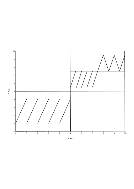
Figure 1. An example of a $1-$dimensional map $T$ with two least elements

In sections 2, 3 and 4 we studied random perturbations of a dynamical system in the framework of general Markov processes. Nevertheless, it is often useful to deal with the case when the Markov process is generated by random transformations [26]. In this setting, we consider an i.i.d. stochastic process $(\omega_{k})_{k\in N}$ with values in $\Omega_{\varepsilon}$ and with probability distribution $\theta_{\varepsilon}$. We associate with each $\omega\in\Omega_{\varepsilon}$ a map $T_{\omega}:M\to M$ and we consider the random orbit starting from the point $x$ and generated by the realization $\underline{\omega}_{n}=(\omega_{1},\omega_{2},\cdots,\omega_{n})$, defined as : $T_{\underline{\omega}_{n}}:=T_{\omega_{n}}\circ\cdots\circ T_{\omega_{1}}(x)$. This defines a Markov process $\mathcal{X}_{\varepsilon}$ with transition function

(5.1) $$P(x,A)=\int_{\Omega_{\varepsilon}}\mathbf{1}_{A}(T_{\omega}(x))d\theta_{\varepsilon}(\omega),$$

where $A\in\mathcal{B}(M)$, $x\in M$ and $\mathbf{1}_{A}$ is the indicator function of a set $A$. The transition function induces an operator ${\mathcal{U}}_{\varepsilon}^{*}$ which acts on measures $\mu$ on $(I,\mathcal{B}(M))$ as:

$${\mathcal{U}}_{\varepsilon}^{*}\mu(A)=\int_{M}\int_{\Omega_{\varepsilon}}\mathbf{1}_{A}(T_{\omega}(x))d\theta_{\varepsilon}(\omega)d\mu(x)=\int_{I}{\mathcal{U}}_{\varepsilon}{\bf 1}_{A}(x)d\mu_{\varepsilon}(x),$$

where ${\mathcal{U}}_{\varepsilon}$ is the random evolution operator acting on $L^{\infty}_{m}$ functions $g$:

(5.2) $${\mathcal{U}}_{\varepsilon}g=\int_{\Omega_{\varepsilon}}g\circ T_{\omega}d\theta_{\varepsilon}(\omega).$$

A measure $\mu_{\varepsilon}$ on $(M,\mathcal{B}(M))$ is called a $\mathcal{X}_{\varepsilon}$-stationary measure if and only if, for any $A\in\mathcal{B}(M)$,

(5.3) $${\mathcal{U}}_{\varepsilon}^{*}\mu_{\varepsilon}(A)=\mu_{\varepsilon}(A).$$

We are interested in studying $\mathcal{X}_{\varepsilon}$-acsm. By (5.2), one can define the transfer operator $\mathcal{L}_{\varepsilon}$ (Perron-Frobenius) acting on $L^{1}(M,\mathcal{B}(M),m)$ by:

(5.4) $$(\mathcal{L}_{\varepsilon}f)(x)=\int_{\Omega_{\varepsilon}}\mathcal{L}_{\omega}f(x)d\theta_{\varepsilon}(\omega),$$

which satisfies the duality condition

(5.5) $$\int_{M}g\mathcal{L}_{\varepsilon}fdm=\int_{M}{\mathcal{U}}_{\varepsilon}gfdm$$

where $g$ is in $L^{\infty}_{m}$ and $\mathcal{L}_{\omega}$ is the transfer operator associated with $T_{\omega}$. It is well know that $\mu_{\varepsilon}:=\rho_{\varepsilon}m$ is a $\mathcal{X}_{\varepsilon}$-acsm if and only if $\mathcal{L}_{\varepsilon}\rho_{\varepsilon}=\rho_{\varepsilon}$; i.e., $\rho_{\varepsilon}$ is a $\mathcal{X}_{\varepsilon}$-invariant density. In order to use the results of sections 2, 3 and 4, we also assume that assumptions (P1), (P2) (B1)-(B3), (LY) and (RLY) hold. Moreover, we assume that (5.4) reduces to

(5.6) $$(\mathcal{L}_{\varepsilon}f)(x)=\int_{\Omega_{\varepsilon}}\mathcal{L}_{\omega}f(x)d\theta_{\varepsilon}(\omega)=\int_{M}p_{\varepsilon}(z,x)f(z)dz.$$

In fact, an important example of a random perturbation where $\mathcal{L}_{\varepsilon}$ can be reduced as in (5.6) is the case of additive noise. For instance if $M=S^{q}$, the $q$-dimensional torus , let define $T_{\omega}=T(x)-\omega$ mod $S^{q}$, where $\omega\in S^{q}$. Let the density of $\theta_{\varepsilon}$ with respect to the Lebesgue measure $d\omega$ on $S^{m}$, $h_{\varepsilon}$, be continuously differentiable with support contained in the square $\Omega_{\varepsilon}\equiv[-\varepsilon,\varepsilon]^{q}$: $\int d\theta_{\varepsilon}=\int h_{\varepsilon}(\omega)d\omega=1$. It is then straightforward to check that $p_{\varepsilon}(x,y)=h_{\varepsilon}(Tx-y)$.

Remark 5.1.

The preceding example illustrates very well the relation between the two approaches used in this paper to deal with randomness. Namely the Markov chain approach, which was used to prove Theorem 1, and the random transformations approach which permits to follow the orbit of a point under the concatenation of the randomly chosen maps. Consequently, the latter allows for more explicit representation of objects like the evolution operator and the transfer operator. In fact, relation (5.6) is a general fact whenever the transition function for the Markov chain is given by the integral (see (5.1)), $P(x,A)=\int_{\Omega_{\varepsilon}}\mathbf{1}_{A}(T_{\omega}(x))d\theta_{\varepsilon}(\omega)$, and the noise is absolutely continuous, namely $\theta_{\epsilon}(\omega\in\Omega_{\epsilon};\ T_{\omega}x\in A)=\int_{A}p_{\epsilon}(x,z)dz$, where $A$ is a measurable set in $M$. This in particular means that we can always construct a Markov chain starting with a random transformation. The converse is also true. We refer to [26] for the construction, and to [21] for recent results in this direction. Finally, we stress that Theorem 1 has been proved for an absolutely continuous noise. This means that it cannot be applied, in its actual form, to random perturbations on a finite noise space, for which the probability $\theta_{\epsilon}$ is an atomic measure and the random transfer operator $\mathcal{L}_{\epsilon}$ applied to the function $f$ becomes a weighted operator of the form $\sum_{j\geq 1}\mathcal{L}_{\omega_{j}}\ f\ p_{\omega_{j}}$, where the weights $p_{\omega_{j}},\ \sum_{j\geq 1}p_{\omega_{j}}=1$, are associated to the values of the random variables $\omega_{j}$.

5.1. $1$-dimensional examples

To illustrate our results, we present two simple examples of $1$-dimensional maps. In these examples the Banach space $\mathcal{B}$ is considered to be the space of functions of bounded variation. In Example 5.2 we present a map that has three ergodic components and two least elements.

Example 5.2.

In this example $T:[0,10]\to[0,10]$. The graph of $T$ is shown in Fig. 1. $T$ is piecewise linear and Markov with respect to the partition:

$$[0,1),\dots,[4,5),[5,5.5)\dots,[9.5,10].$$

One can easily check that $T$ has exactly three ergodic acim whose supports $\Lambda_{1},\Lambda_{2},\Lambda_{3}$ are, respectively, equal to $[1,4]$, $[5.5,7.5]$, and $[7.5,9.5]$. Moreover, one can easily check that $T$ admits two least elements. Namely, $\{\Lambda_{1}\}$ and $\{\Lambda_{2},\Lambda_{3}\}$.

5.2. A $2$-dimensional example

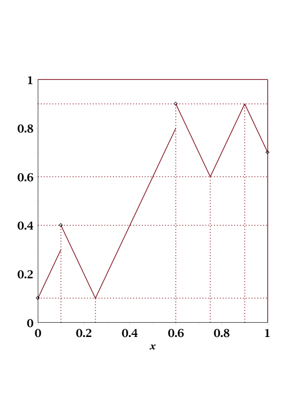
Figure 2. The graph of the map $T$ for $a=0.1$. The least element for $T$ is the closed interval $[\frac{1}{2}+a,1-a]$. This induces the least element $[\frac{1}{2}+a,1-a]\times S$ for $\Phi_{0}$ on $[0,1]\times S$.

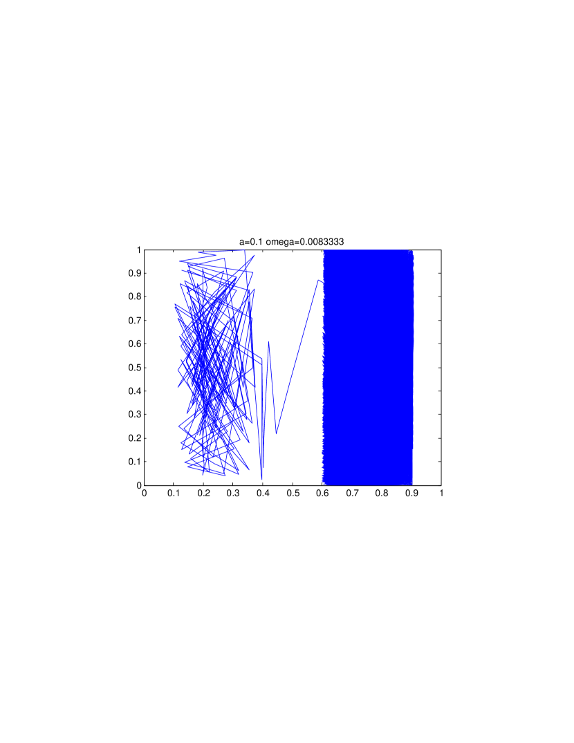
Figure 3. The least element on the right side $x>\frac{1}{2}$ for the map $\Phi_{\omega}$; notice that $\omega$ on the top of the figure is just $\epsilon=1/120.$

Example 5.3.

We now present an example in higher dimensions, in particular the two-dimensional skew system $\Phi_{\omega}:[0,1]\times S\rightarrow[0,1]\times S$ defined as $(x^{\prime},y^{\prime})=\Phi_{\omega}(x,y)$ where

$$x^{\prime}=T(x)+\omega y$$

$$y^{\prime}=2y\ \text{ mod}1,$$

where $S$ denotes the unit circle, and $T:[0,1]\to[0,1]$ is given by

• for $x\in[0,a),\ T(x)=(\frac{1}{2a}-3)x+a$;

• for $x\in[a,\frac{1}{4}),\ T(x)=-2x+(a+\frac{1}{2})$;

• for $x\in[\frac{1}{4},\frac{1}{2}+a),\ T(x)=2x+(a-\frac{1}{2})$;

• for $x\in[\frac{1}{2}+a,\frac{3}{4}),T(x)=-2x+(2+a)$;

• for $x\in[\frac{3}{4},1-a),T(x)=2x+(a-1)$;

• for $x\in[1-a,1],T(x)=(3-\frac{1}{2a})x+(-\frac{5}{2}+\frac{1}{2a}+2a)$.

The graph of $T$ is depicted in Fig.2

We considered a piecewise linear map to simply the exposition. However, this is not really needed to apply our results. In fact, a map with nonlinear branches can be used in the example as long as we keep uniform dilatation, bounded distortion, and a $C^{1+}$ smoothness. For each $\omega$ we have a different random map and we compose them by taking $\omega$ uniformly distributed, for instance, between $(-\epsilon,\epsilon)$. In this case $\theta_{\epsilon}(\omega)=\frac{1}{2\epsilon}d\omega$. The positive parameter $a$ can be chosen equal to $\frac{1}{10}$, in such a way that the image of the unit interval remains in $[0,1]$ when $\epsilon<a$. It is very easy to check that the unperturbed map $\Phi_{0}$ has two ergodic components which are, respectively, subsets of $[a,\frac{1}{2}-a]\times S$ and $[\frac{1}{2}+a,1-a]\times S$ and the latter is a least element. These ergodic components are with respect to absolutely continuous invariant measures whose densities are the fixed points of the Perron-Frobenius operator associated to $\Phi_{0}$. The existence of such fixed points follow easily by obtaining a Lasota-Yorke inequality on a suitable function space, such as the space of functions of bounded variation [9] or quasi-Hölder functions, [29, 19], which satisfy all the assumptions required in this paper. Notice that a Lasota-Yorke inequality can be obtained as well for the random Perron-Frobenius operator associated to the random system, by using the closeness of the perturbed maps $\Phi_{\omega},\ |\omega|\leq\epsilon$ for small $\epsilon$ (this means that the constants $\eta$ and $D$ in (LY) and (RLY) can be chosen to be the same for the unperturbed and the perturbed systems). According to our main theorem, there must be only one ergodic absolutely continuous stationary measure and this must be supported in a neighborhood of the least element. In Fig. 4 we show the limit set of several random orbits taken with $\epsilon=1/120$ and $a=0.1$. All these random orbits accumulate in the right hand side of $[0,1]\times S$ as predicted by our theory.

References

- [1] Alves, J.F., Araujo, V., Random perturbations of nonuniformly expanding maps, Astérisque, 286, (2003), 25–62.
- [2] Aytac, H., Freitas, J., Vaienti, S. Laws of rare events for deterministic and random dynamical systems. Submitted. Available at arxiv.org/pdf/1207.5188.
- [3] Bahsoun, W. , Vaienti, S. Metastability of certain intermittent maps. Nonlinearity, 25 (2012), no. 1, 107–124.
- [4] Bahsoun, W, Vaienti, S., Escape rates formulae and metastability for randomly perturbed maps. Nonlinearity, 26 (2013), 1415–1438.
- [5] Baladi, V. Positive transfer operators and decay of correlations. Advanced Series in Nonlinear Dynamics, 16. World Sci. Publ., NJ, 2000.
- [6] Baladi, V., Gouëzel, S. Good Banach spaces for piecewise hyperbolic maps via interpolation. Ann. Inst. H. Poincaré Anal. Non Linéaire 26 (2009), no. 4, 1453–1481.
- [7] Baladi, V., Young, L.-S. On the spectra of randomly perturbed expanding maps. Comm. Math. Phys. 156 (1993), no. 2, 355–385.
- [8] Bonatti, Christian; Daz, Lorenzo J.; Viana, Marcelo, Dynamics beyond uniform hyperbolicity. A global geometric and probabilistic perspective. Encyclopaedia of Mathematical Sciences, 102. Mathematical Physics, III. Springer-Verlag, Berlin, 2005.
- [9] Boyarsky, A., Gora, P., Laws of Chaos, Invariant measures and Dynamical Systems in one dimension, Birkhäuser, (1997).
- [10] Cowieson, W., Stochastic stability for piecewise expanding maps in , Nonlinearity, 13, (2000), 1745-1760.
- [11] Dellnitz, M., Froyland, G., Horenkamp, C., Padberg-Gehle, K., and Sen Gupta, A. Seasonal variability of the subpolar gyres in the Southern Ocean: a numerical investigation based on transfer operators. Nonlinear Processes in Geophysics, 16:655-664, (2009).
- [12] Demers, M., Liverani, C., Stability of statistical properties in two-dimensional piecewise hyperbolic maps. Trans. Am. Math. Soc., 360 (2008), 4777–4814.
- [13] M. Demers and H.-K. Zhang, Spectral analysis of the transfer operator for the Lorentz Gas, Journal of Modern Dynamics 5, (2011), 665-709.
- [14] Dolgopyat, D., Wright, P. The Diffusion Coefficient for Piecewise Expanding Maps of the Interval with Metastable States. Stochastics and Dynamics, 12 (2012), no. 1, 1150005, 13 pp.
- [15] Froyland, G., Stancevic, O. Escape rates and Perron-Frobenius operators: open and closed dynamical systems. Discrete Contin. Dyn. Syst. Ser. B 14 (2010), no. 2, 457–472.
- [16] Froyland, G. and Stancevic, O. Metastability, Lyapunov exponents, escape rates, and topological entropy in random dynamical systems. Stochastics and Dynamics, 13, (2013) 1–26.
- [17] Gonzaléz-Tokman, C., Hunt, B., Wright, P. Approximating invariant densities for metastable systems, Ergod. Th. Dynam. Sys. (2011), 31, 1345–1361.
- [18] Hennion, H., Hervé, L., Limit theorems for Markov chains and Stochastic Properties of Dynamical Systems by Quasicompactness, Lect. Notes Math., 1766, (2001), Springer-Verlag.
- [19] Hu, H., Vaienti, S. Absolutely continuous invariant measures for non-uniformly expanding maps. Ergod. Th. Dynam. Sys, 29 (2009), 1185–1215.
- [20] Ionescu-Tulcea, C.T., Marinescu, G. Théorie ergodique pour des classes d’opérateurs non complétement continus. Ann. Math. (1950), 52 (2), 140–147.
- [21] Jost, J., Kell, M. and Rodrigues, C. Representation of Markov chains by random maps: existence and regularity conditions. Available on http://arxiv.org/pdf/1207.5003.pdf
- [22] Keller, G. Stochastic stability in some chaotic dynamical systems. Monatsh. Math. 94 (1982), no. 4, 313–333.
- [23] Keller, G., Liverani, C. Stability of the spectrum for transfer operators. Ann. Scuola Norm. Sup. Pisa Cl. Sci. (4) 28 (1999), no. 1, 141–152.
- [24] Keller, G. and Liverani, C. Rare events, escape rates, quasistationarity: some exact formulae. J. Stat. Phys., 135 (2009), no. 3, 519–534.
- [25] Kifer, Y. Attractors via random perturbations, Commun. Math. Phys., (1989), 445–455.
- [26] Kifer, Y. Ergodic theory of random transformations, Birkhäuser, 1986.
- [27] Liverani, C. Multidimensional expanding maps with singularities: a pedestrian approach. Ergod. Th. Dynam. Sys. 33 (2013), no. 1, 168–182.
- [28] Ruelle, D. Small random perturbations of dynamical systems and the definition of attractors, Commun. Math. Phys., (1981), 82, 137–151.
- [29] Saussol, B., Absolutely continuous invariant measures for multidimensional maps, Israel Jour. Math., 116, (2000), 223–248.
- [30] Santitissadeekorn, N., Froyland, G., and Monahan, A. Optimally coherent sets in geophysical flows: A new approach to delimiting the stratospheric polar vortex. Phys. Rev. E, (2010), 056311-6.