Measuring Propagation Speed of Coulomb Fields

Abstract

The problem of gravity propagation has been subject of discussion for quite a long time: Newton, Laplace and, in relatively more modern times, Eddington pointed out that, if gravity propagated with finite velocity, planet motion around the sun would become unstable due to a torque originating from time lag of the gravitational interactions.

Such an odd behavior can be found also in electromagnetism, when one computes the propagation of the electric fields generated by a set of uniformly moving charges. As a matter of fact the Liénard-Weichert retarded potential leads to the same formula as the one obtained assuming that the electric field propagates with infinite velocity. The Feynman explanation for this apparent paradox was based on the fact that uniform motions last indefinitely.

To verify such an explanation, we performed an experiment to measure the time/space evolution of the electric field generated by an uniformly moving electron beam. The results we obtain, on a finite lifetime kinematical state, are compatible with an electric field rigidly carried by the beam itself.

1 Introduction

In Space, Time and Gravitation Eddington discusses [1] the problem of gravity propagation. He remarks that if gravity propagated with finite velocity the motion of the planets around the Sun would become unstable, due to a torque acting on the planets. The problem was already known to Newton and was examined by Laplace [2], who calculated a lower limit for the gravity propagation velocity, finding a value much larger than the speed of light.

However, at the time of Eddington’s writing, General Relativity had been just formulated, with gravitational waves traveling with the speed of light as a possible solution. Eddington noted that a similar problem existed in electromagnetism, and since electromagnetic waves in vacuum do travel with the speed of light, he concluded that in General Relativity gravity also propagates with the speed of light.

We remark that an intriguing behavior of electromagnetism occurs when the field of an electric charge moving with constant velocity is computed. One finds that in such a case the electric field at a given point $\boldsymbol{P(x,y,z,t)}$ evaluated with the Liénard-Wiechert (L.W.) potentials is identical to that calculated by assuming that the Coulomb field travels with infinite velocity.

This is a direct consequence of the velocity field, the part of the L.W. potentials independent of the charge acceleration, being a static field. This feature has been strassed by several authors e.g. [5] [6]. The Feynman [3] interpretation is based instead on the assumption that the uniform motion lasts indefinitely and that an observer would see an angular acceleration of the approaching charge.

The only way to shed some light on this problem, either the Feynman interpretation or the static Coulomb field carried rigidly by the charge is by means of an experiment.

To verify if the Feynman interpretation of the L.W. potentials holds in case of a charge moving with constant velocity for a finite time, we have performed an experiment to measure the time evolution of the electric field produced by an electron beam in our laboratory; such kinematic state has obviously a finite lifetime.

It is well known that a sizable number of instrumentation devices (e.g. beam position monitors) are based on effects produced by electric fields carried by particle beams. The effects and the propagation of such fields, however, have never been studied in details: the main point exploited by these devices is that the field effects are contemporary to the particles passage and that the signal size obtained, for instance, on a pair of strip-lines inside a vacuum pipe yields a measurement of the transverse position of the beam itself. The experimental situation for those devices is quite complicated to understand, as all the fields are inside a conductor and the transverse distances exploited are always small. We, on the contrary, tried to carry out our experiment in a clean environment: the electron beams used were propagating in a vacuum like environment. We covered a wide range of transverse distances w.r.t. the beam line (up to 55 cm). Such range leads to explore time and space domains for the emission of the detected field far outside the physical region.

The data we collected, as shown in the following, are compatible with the hypothesis of a Coulonb filed carried rigidly by the moving charge

2 Theoretical Considerations

The electric field at ${\boldsymbol{r}}(x,y,z)$ from a charge $e$ traveling with constant velocity $\boldsymbol{v}$, at a time $t$ can be written, using the Liénard-Wiechert retarded potentials as [4, 5, 6]:

$${\boldsymbol{E}}({\boldsymbol{r}},t)=\frac{e}{4\pi\epsilon_{o}}\frac{1-{v^{2}}/{c^{2}}}{\left(R(t^{\prime})-\frac{{\boldsymbol{R}}(t^{\prime})\cdot{\boldsymbol{v}}}{c}\right)^{3}}\left({\boldsymbol{R}}(t^{\prime})-{\boldsymbol{v}}\frac{R(t^{\prime})}{c}\right),$$ (1)

where

$${\boldsymbol{R}}(t^{\prime})={\boldsymbol{r}}-{\boldsymbol{v}}t^{\prime}$$ (2)

is the distance between the moving charge and the space point where one measures the field at time $t$, and

$$t^{\prime}=t-\frac{R(t^{\prime})}{c}.$$ (3)

The field from a steadily moving charge can also be written (as easily deducible from Eq. 1 in case of constant velocity) [3, 4, 5, 6] as

$${\boldsymbol{E}}(t)=\frac{e}{4\pi\epsilon_{o}}\frac{{\boldsymbol{R}}(t)}{R(t)^{3}}\frac{1-{v^{2}}/{c^{2}}}{(1-\frac{v^{2}}{c^{2}}sin^{2}(\theta(t))^{\frac{3}{2}}}$$ (4)

where $\boldsymbol{R}(t)$ is the vector joining the charge position and the point at which we evaluate the e.m. field at time $t$ (Eqs. 38.8 and 38.9 of [4]) and $\theta(t)$ is the angle between $\boldsymbol{v}$ and $\boldsymbol{R}(t)$

A pictorial view of the above mentioned quantities can be seen in Fig.1.

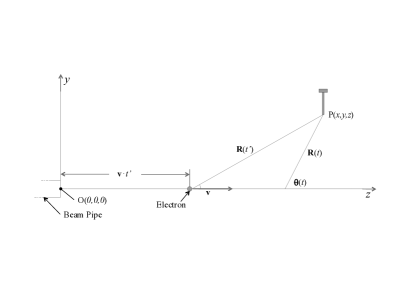
Figure 1: A pictorial view of various quantities mentioned in eqns 1 and 4.

If we indicate with $y$ the generic transverse coordinate, using eqn.1 we can compute the maximum transverse electric field w.r.t. the direction of motion, given by ($\gamma\equiv 1/\sqrt{1-v^{2}/c^{2}}$):

$$E_{max}=\frac{e}{4\pi\epsilon_{o}}\frac{\gamma}{y^{2}},$$ (5)

a value obtained when the charge is at a distance $\gamma y$ at a time

$$t^{\prime}=t-\frac{\gamma y}{c}$$ (6)

.

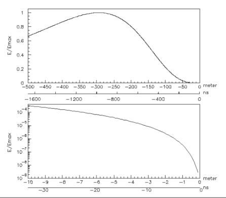
Figure 2: The electric field from eqn. 1 normalized to its maximum value, ${E_{y}(R)}/{E_{max}}$, generated by 500 MeV electrons as a function of $z^{\prime}$ (or $t^{\prime}$, lower abscissa scales), expected at $(z=0{\rm\,cm},y=30{\rm\,cm})$. $z^{\prime}$ and $t^{\prime}$ are defined in eqns. 2 and 3. The horizontal scale of the upper graph (a) is such to include the point where ${E_{y}(R)}={E_{max}}$; the lower graph (b) is a close-up of the region $z\in[-10,0]\,$m typical of our experiment (note the different vertical scales).

Fig. 2 shows the field, normalized to $E_{max}$, generated by relativistic electrons ($E=500\,$MeV) moving along the $z$ axis, at a transverse distance $y=30\,$cm. We observe that the maximum value of the field appears to be generated when the charges are in an unphysical region, namely $z=-300\,$m. Conversely, the calculated electric field in the region of our experiment ($|z|\leq 10\,$m) is many orders of magnitude smaller.

3 The Experiment

In our experiment we measure the electric field generated by the electron beam produced at the DA$\Phi$NE Beam Test Facility (BTF) [7], a beam line built and operated at the Frascati National Laboratory to produce a well-defined number of electrons (or positrons) with energies between 50 and 800 MeV. At maximum intensity the facility yields, at a 50 Hz repetition rate, 10 nsec long beams with a total charge up to several hundreds pCoulomb. The electron beam is delivered to the 7 m long experimental hall in a beam pipe of about 10 ${\rm\,cm}$ diameter, closed by a $40\,\mu$m Kapton window. Test were carried out shielding the exit window with a thin copper layer, but we did not observe any change in the experimental situation. At the end of the hall a lead beam dump absorbs the beam particles. In our measurements we used 500 MeV beams of $0.5\div 5.0\times 10^{8}$ electrons/pulse ($\gamma\simeq 10^{3}$).

A schematic view of the experimental setup is shown in Fig. 3. At the beam pipe exit flange, electrons go through a fast toroidal transformer measuring total charge and providing redundancy on our LINAC-RF based trigger.

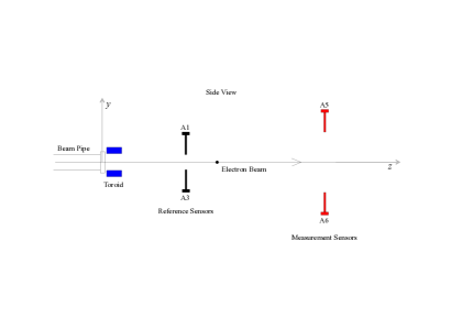
Figure 3: A schematic side viewof our experimental apparatus. Sensors A2 and A4, orthogonal to the figure plane, are not shown.

To measure the electric field we used as sensors 14.5 ${\rm\,cm}$ long, 0.5 ${\rm\,cm}$ diameter Copper round bars, connected to our Data Acquisition System by means of fast, terminated coax cables.

To record the sensors waveforms we used a Switched Capacitor Array (SCA) circuit (CAEN mod V1472) able to sample the input signal at 5 GHz. In addition to the sensors output, the SCA stored also the LINAC-RF trigger and the toroid pulse.

The Coulomb field acts on our sensor quasi-free electrons, generating a current. An example of the recorded signals is shown in Fig.4.

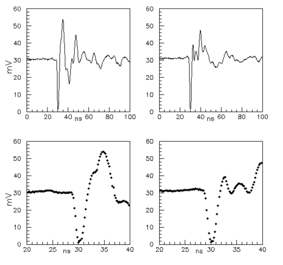
Figure 4: Typical A5 (left) and A6 (right) sensor responses. The lower plots show in detail the granularity of our time measurements (200 psec./bin).

The pulse shape which, unlike the current intensity, depends on the inductance, capacitance and resistance (L, C, R) of the detectors.

The sensor response $V(t)$ for a step excitation $V_{0}$ can be written as:

$$V(t)=V_{o}\cdot e^{-\frac{R}{2L}t}sin(\omega t).$$ (7)

The natural frequency of the detectors is $\approx$ 250 MHz. The voltage difference between the bar ends for the maximum value of the Coulomb field, obtained suitably modifying eqn. 5 for a finite longitudinal extent of the charge distribution (in our case, the electron beam is $\approx$ 3 m. long) is:

$$V^{t}_{max}=\eta\frac{\lambda}{2\pi\epsilon_{o}}ln\left(\frac{y+14.5~{}cm}{y}\right),$$ (8)

where $\lambda$ is the charge per unit length of the incoming beam and $\eta$ is the sensor calibration constant. In the electric field calculations, the image charges appearing on the flange as the beam exits the pipe have also been included. However, as their effect decreases rapidly with the distance from the flange, it is completely negligible in our experiment (distance$\geqslant 1\,$m). The sensor calibration has been carried out using a known field generated by a parallel plate capacitor. We find experimentally $\eta=7.5\times 10^{-2}\pm\ 3\%$, however due to various systematic effects we believe our calibration to be good to $\approx$ 20%, in absolute terms.

Assuming that the L.W. formula in eqn. 8 holds (which should apply only if the uniform charge motion would last indefinitely and the charges generating the field would not be shielded by conductors) we expect, in our typical beam operating conditions, pulse heights of the order of 10 mV out of our sensors. In the more realistic hypothesis that the L.W. formula should be corrected to take into account the beam pipe shielding and the finite lifetime for the charges uniform motion, as it is in our experiment, the expected amplitude, cfr. fig.2, would be of the order of few nanoVolt and hence unmeasurable.

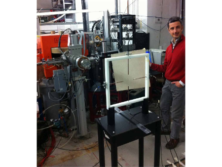
Figure 5: A photograph of the beam pipe exit window and of the four reference sensors in the cross configuration.

We used six sensors: four of them, A1, A2, A3 and A4 in the following, are located at a longitudinal distance of 92 cm from the beam exit flange in a cross configuration, each at a transverse distance of 5 cm from the beam line (cfr. fig. 5). The main purpose of these four sensors is to provide reference for the other two detectors A5 and A6 located through out the measurements at various longitudinal and transverse coordinates along the beam trajectory.

4 Measurements and data base

Electron beams were delivered by BTF operators at a rate of few Hertz; data were collected in different runs, identified by given longitudinal and transverse position of the movable detectors (A5 and A6).

We collected a total of eighteen runs, spanning six transverse positions and three longitudinal positions of A5 and A6 for a total of about 15,000 triggers. Through out the data taking, the references sensors (A1,A2,A3,A4) were left at the same location (92 cm. from the beam exit flange) in order to extract a timing and amplitude reference. As mentioned before, we collected data with the movable sensor at 172 cm, 329.5 cm and 552.5 cm longitudinal distance from the beam exit flange. For each of the longitudinal positions we collected data on six transverse positions: 3, 5, 10, 20, 40 and 55 cm from the nominal beam line. For each run, A5 and A6 were positioned symmetrically with respect to the nominal beam line; spatial precision in the sensor positioning was of the order of few mm in the longitudinal coordinate and 1 mm in the transverse one.

We define:

$${\bf Sn}=\frac{V_{max}\times 10^{8}}{N_{elec}},$$ (9)

where $V_{max}$ is the peak signal recorded by the SCA and $N_{elec.}$ is the total number of electrons in the beam, as measured by the fast toroid. The factor $10^{8}$ in eqn.9 takes into account the typical beam charge.

Figure 6: Normalized amplitude Sn (see text for details) for sensor A1 in two different runs: the above mentioned sensor was in the same operating conditions through out the different runs, taken minutes apart.

As an example, the two plots in Fig. 6 show the Sn values for the reference sensor A1, for two different runs. One issue common to all our measurements stands out clearly: in the same experimental conditions (sensor position, trigger timing, cable lengths, DAQ settings) the two distributions are different. We attribute this difference to less than perfect reliability in the beam delivery conditions (launch angles, total beam length, charge distribution in the beam pulse length, stray magnetic fields, etc.), over which we had little control.

Since our four reference sensors must provide normalization for the measurements taken by A5 and A6, our analysis proceeds as follows. We obtain, on a run-by-run basis, the average amplitude of the four reference sensors, either evaluating the medians, or fitting the distributions with Gaussian functions and taking the mean values.

Next we make the assumption that in any given series of runs under study, different only for the position of the movable sensors A5 and A6, each reference sensor, that is never moved, must always yield the same amplitude. Since Fig. 6 shows that this is not the case, we need to allow for some (uncontrolled) effect due to variation of beam parameters. We do so by enlarging the errors on the reference amplitudes, originating from the Gaussian fits, by a rescaling factor. This factor is chosen by requesting that the reduced $\chi^{2}$ of the series be consistent with the hypothesis that all amplitude measurements for any given sensor in the series have one common value.

Once obtained the error rescaling factor, for a given sensor and run series, we proceed to analyze the movable detectors by enlarging by the same factor their own uncertainties. The amount of rescaling needed is of the order of 10; the overall relative error on the run-averaged pulse height is typically $\approx$ 10%.

4.1 Amplitude as a function of transverse distance

As mentioned in the previous section, at each longitudinal position we collected data at six different transverse positions for A5 and A6. The requirements placed on data were: a lower cut on the beam charge ($N_{e}>0.5\times 10^{8}$) and upper cut on the baseline noise on the six detectors (noise $<$ 0.5 mV , where the typical r.m.s. noise was 0.15 mV). We select in this way roughly 70% of the recorded triggers.

Fig. 7, 8 and 9 show normalized amplitudes Sn versus transverse distance obtained for the three different longitudinal positions. The displayed results are completely consistent with eqn.8, which gives the voltage value expected in case of a charge indefinitely moving with constant speed.

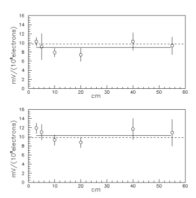
Figure 7: Comparison between measurements and predictions from eqn 8: normalized amplitudes Sn for sensors A1(upper) and A3(lower) for $z_{A5,A6}$ =172.0 cm. The continuous line at 8.98$\pm$0.54 mV (upper) and 10.25$\pm$0.59 mV (lower) indicate the weighted average of our measurements. The six measurements plotted refer to the transverse positions of sensor A5, A6. No dependence is expected (see text), as sensor A1, A3 were kept in the same operating conditions and at the same locations. The dashed line indicates the nominal normalized value $V^{t}_{max}=9.78~{}mV$ of eqn.8 for y=5 cm. The agreement between measurements and prediction is remarkable

Figure 8: The same plot as in fig.7 at $z_{A5,A6}$= 329.5 cm. The continuous lines at 8.80 $\pm$0.63 mV (upper) and 10.47$\pm$0.86 (lower) indicate the weighted average of our measurements.

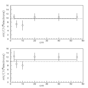
Figure 9: The same plot as in fig.7 at $z_{A5,A6}$ = 552.5 cm. The continuous line at 9.67 $\pm$0.54 mV (upper) and 10.75$\pm$0.74 (lower) indicate the weighted average of our measurements.

The results shown in fig 7, 8 and 9 were obtained without any normalization between measurements and L.W. theory. We stress again that the amplitude we measure is many orders of magnitude higher than that one would expect from the unshielded beam charge. Were we sensitive only to fields generated by the electron beam once they exited the beam pipe, our pulse height would have been, as mentioned in the previous paragraph, in the few nanoVolt range and then undetectable.

In figg. 10, 11 and 12 we show the amplitude ratios between sensors A5 and A1 (A6 and A3) as a function of transverse distance from the beam line. Also in this case, data are completely consistent with the logarithmic behavior of eqn 8.

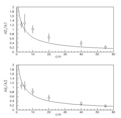
Figure 10: Upper graph: the points show the ratio $V_{max}(A5)\over V_{max}(A1)$ at z_A5,A6=172.0 cm versus the transverse distance. Lower graph: $V_{max}(A6)\over V_{max}(A3)$. The continuous lines represent eqn. 8 for the depicted ratios. The two reduced $\chi^{2}$ are respectively 1.82 and 1.06. No fit has been performed on the data: the reduced $\chi^{2}$ has been evaluated from eqn 8 and the experimental data.

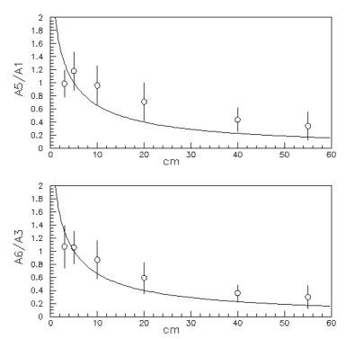
Figure 11: The same plot as in fig.10 at z_A5,A6=329.5 cm. The two reduced $\chi^{2}$ are respectively 1.36 and 0.66.

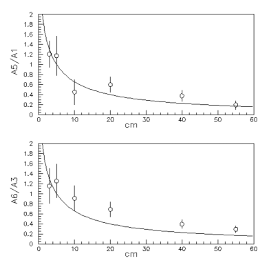
Figure 12: The same plot as in fig.10 at z_A5,A6=552.5 cm The two reduced $\chi^{2}$ are respectively 0.91 and 2.48.

4.2 Timing measurements

Our 200 psec/chn SCA provides timing for detector outputs, so that it is possible to detect both longitudinal and transverse position-time correlations. As a reminder we stress again that, in the hypothesis of stationary constant speed motion, no time difference is expected as a function of transverse distance, while different longitudinal positions should exhibit delays consistent with particles traveling at $\gamma\approx$ 1000.

Also in this case, we will have to rescale the errors yielded by standard procedures extracting central values from quasi Gaussian distributions; in this case we impose that, by symmetry, the time difference between A5 and A6 be independent from the transverse distance between detector and nominal beam line. We then duplicate the procedure described in the previous section requiring that time difference between A5 and A6 for each run all come from a common value.

Figure 13: Top graph: time difference between A5 and A6 versus the transverse distance. Errors have been rescaled according to the procedure described in the text. Middle and bottom plots: time difference between the movable sensors A5 and A6 (respectively) and one of the fixed sensors, A1. $z_{A5,A6}$ = 172 cm. The line at 1.549$\pm$0.036 nsec.(middle) and 1.500$\pm$0.036 nsec (lower) indicate the weighted average of our measurements, once the reduced $\chi^{2}$ is rescaled according to the procedure described in the text (par. 4.2). The values obtained for the A5-A1, A6-A1 absolute delays have to be corrected for the cables different lengths ($\approx$ 1 nsec.).

The upper graph of fig 13 shows the time difference relative to 172 cm longitudinal distance data. The amount of rescaling, in this case, is about a factor of 10 and the overall resolution on time difference measurements is of the order of 50 psec.

The data show no time dependence of the sensor signal on transverse distance: the reduced $\chi^{2}$ for the hypothesis of a constant delay as function of $y$ is always below 2 at each longitudinal positions. Furthermore, would one add a linear term depending on transverse distance for the sensor time delay, the inverse velocity obtained would have a value smaller than $3\times 10^{-9}$ $sec\over m$ at 95% confidence level.

We summarize the time distance correlations in Table 1, where the data obtained at the three different longitudinal positions are shown.

Table 1: Timing measurements. The expected differences are calculated for 500 MeV electrons.

longitudinal distances	expected	experimental	experimental
between two sensors [cm]	[ns]	a5 [ns]	a6 [ns]
(552.5-329.5) 223.0$\pm 1.5$	$7.43\pm 0.05$	$7.28\pm 0.02$	$7.52\pm 0.04$
(552.5-172.0) 380.5$\pm 1.5$	$12.68\pm 0.05$	$12.62\pm 0.04$	$12.84\pm 0.05$
(329.5-172.0) 157.5 $\pm 15.$	$5.19\pm 0.05$	$5.21\pm 0.03$	$5.17\pm 0.04$

4.3 E.M. Backgrounds

We preformed different tests in order to ascertain that E.M. radiation coming from the interaction of the electron beam with its environment was not the original cause of our sensors’ response.

With the beam steering system, we changed the launch angle in the experimental hall; varying the current of the beam line magnet(s) one can then predict the amplitude ratio of two detectors located right and left of the beam line, according to the calculated beam position at the sensors’ longitudinal coordinates. Special runs were taken to this purpose and the results are completely consistent with the expected horizontal beam displacement w.r.t. the nominal position.

Other E.M. phenomena are related to boundary crossings: as the beam travels between different media (e.g. the beam exit flange) E.M. radiation can be generated. This, in turn, might mimic pulses we assume due to the interaction of the beam itself with our sensors. The experimental situation can be schematized as a Tamm [8] problem: a beam of particles traveling inside the vacuum pipe of the Linac, suddenly appears out of the end flange of the accelerator, moves with uniform velocity through out the experimental hall ($\approx$ 7 m.) and disappears in the concrete wall of the hall. A calculation of the expected effect, using the formulae reported in [9] lent us confidence that this background was not extremely relevant; however, in order to demonstrate that such a phenomenon does not contribute (or contributes very little) to our sensors’ signal, we had a dedicated run during April 2014.

We collected data in two different modes:

1. Calibration runs in order to match the data collected during the 2012 campaign to the latest (2014) runs.

2. Beam dump runs in which the electron beam was stopped in a 40 X₀ lead dump before reaching the vertical detectors A5 and A6.

The underlying idea was that data taken with the beam dump, would yield the response of the A5, A6 detectors in a no-beam situation thus allowing us to map the pulse height of our detectors when just backgrounds were present in the experimental hall.

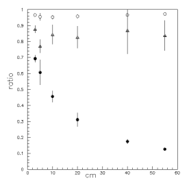
Figure 14: Amplitude ratios vs transverse distance of sensors A5,A6 for calibration runs: open circles A1 A3 ratio, triangles A5 A6 ratio, full dots A5 A1 ratio. The plot is completely consistent with results described in sec 4.1

From fig.14 one can infer that the main features of the previous (2012) measurements are retained in the (2014) latest run; small difference in the absolute values for the given ratios can be attributed to a less the perfect alignment of the two sets of detector on the beam line.

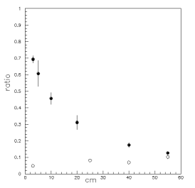
Figure 15: Amplitude ratio for sensor A5 A1 vs (A5) transverse distance from the beam line: full dots calibration runs; circles runs taken with the beam dump inserted between A1…A4 and A5, A6. Open circles data show unequivocally that any e.m. radiation originating either at the beam pipe boundaty or at the beam dump entrance does not score on our detectors.

Fig 15 shows the comparison between data taken in the calibration mode and the beam dump mode, that is when the 40 X₀ lead absorber is inserted between the A1…A4 and the A5,A6 sensors. The vertical sensors responses are, with the beam dump in place, reduced by a factor $\approx$ 10, at 5 cm (transverse) distance, with practically no dependence on (transverse) distance from the beam line. Such behavior lends itself to the interpretation that the overall amount of E.M. background originating either at the transition flange or at the beam dump entrance is indeed small w.r.t. the response obtained when beams unimpeded go through the experimental hall.

5 Discussion

With reference to table 1, we notice that the longitudinal time differences are completely consistent with the hypothesis of a beam traveling along the $z$ axis with a Lorentz factor $\gamma\approx 1000$.

Such an occurrence agrees with the Liénard-Weichert model. Retarded potentials, however, predict that most of the virtual photons [10] responsible for the field detected at coordinates $z$ and $y$ be emitted several hundred meters before the sensor positions and at different times according to the detectors transverse distances. Conversely, assuming that such virtual photons are emitted in a physically meaningful region (between the beam exit window and our detectors), the amplitude response of the sensors should be several order of magnitude smaller than what is being measured (cfr. Fig.2). Our result, obtained with a well definite set of boundary conditions (longitudinal and transverse distance between beam line and sensors, details of the beam delivery to the experimental hall etc.) matches precisely (within the experimental uncertainties) the expected value of the maximum field calculated according to L.W. theory, that is also the value calculated with Eq.4 when the beam is at the minimum distance from the sensor.

We again point out that the consistency of our measurement and eqn 8 has been obtained without any kind of normalization.

6 Conclusions

The data we have discussed in the previous paragraphs led us to assume that the electric field of the electron beams acts on our sensors only after the beam itself has exited the beam pipe and that Cerenkov and/or transition radiation effects are negligible.

Our results agree with the prediction of L.W.formula, however if equation 1 is intended as if the fields were launched at an earlier time with respect to the sensors’ response, such response would be orders of magnitudes smaller than the ones we measure. The Feynman interpretation of the L.W. formula for uniformly moving charges does not show consistency with our experimental data. Even if the steady state charge motion in our experiment lasted few tens of nanoseconds, our measurements indicate that everything behaves as if this state lasted for much longer.

To summarize our finding in few words, one might say that the data do not agree with the most common interpretation of the Liénard-Weichert potential, while seem to support the idea of a Coulomb field carried rigidly by the electron beam.

7 Acknowledgments

We gratefully acknowledge Angelo Loinger for stimulating discussions, Ugo Amaldi for his interest in this research line and his advice, Antonio Degasperis for cross-checking several calculations and Francesco Ronga pointing out and discussing Cerenkov and transition radiation effects. We are indebted with Carlo Rovelli for his criticism and valuable suggestions. We thank Giorgio Salvini for his interest in this research.

We stress as well the relevant contribution of our colleagues from the Frascati National Laboratory Accelerator Division and in particular of Bruno Buonomo and Giovanni Mazzitelli. Technical support of Giuseppe Mazzenga and Giuseppe Pileggi was also very valuable in the preparation and running of the experiment. A special acknowledgment is in order for Paolo Valente, who in different stages of the experiment, has provided, with his advice and ingenuity, solutions for various experimental challenges we faced.

References

-
[1]
A.Eddington Space, Time and Gravitation,
Harper Torchbooks, pag 94 (1959) -
[2]
Laplace, P., Mechanique Celeste , volumes published from 1799-1825, English
translation reprinted by Chelsea Publ., New York (1966)
. -
[3]
R. Feynman, R.B. Leighton, M.L. Sands, The Feynman Lectures on Physics,
Addison-Wesley, Redwood City, vol. II, Chapters 21 and 26.2 (1989)
-
[4]
L.D.Landau and E.M.Lifshitz The classical theory of fields, pag.162,
Pergamon Press, Oxford (1971)
-
[5]
R.Becker Teoria della elettricità, pagg. 73-77
Sansoni Ed. Scientifiche (1950)
-
[6]
J.D.Jackson Classical Electrodynamics, pagg. 654-658
John Wiley & Sons Inc. (1962,1975)
-
[7]
A. Ghigo, G. Mazzitelli, F. Sannibale, P.Valente, G. Vignola
N.I.M. A515 524-542 (2003)
-
[8]
I.E. Tamm Jour. Phys. USSR 1 439 1939
-
[9]
D. Garcia-Fernandez, J. Alvarez-Muniz, W. R. Carvalho, A. Romero-Wolf and E. Zas,
“Calculations of electric fields for radio detection of Ultra-High Energy particles,”
Phys. Rev. D 87, 023003 (2013)
[arXiv:1210.1052 [astro-ph.HE]]
-
[10]
W. K. H.. Panofsky and M. Philips,, Classical
Electricity and Magnetism pagg. 350-351
Addison Wesley Publishing Co.(1955, 1962)