Pairing correlations in exotic nuclei

Abstract

The BCS and HFB theories which can accommodate the pairing correlations in the ground states of atomic nuclei are presented. As an application of the pairing theories , we investigate the spatial extension of weakly bound Ne and C isotopes by taking into account the pairing correlation with the Hartree-Fock-Bogoliubov (HFB) method and a 3-body model, respectively. We show that the odd-even staggering in the reaction cross sections of ^30,31,32Ne and ^14,15,16C are successfully reproduced, and thus the staggering can be attributed to the unique role of pairing correlations in nuclei far from the stability line. A correlation between a one-neutron separation energy and the anti-halo effect is demonstrated for $s$- and $p$-waves using the HFB wave functions. We also propose effective density-dependent pairing interactions which reproduce both the neutron-neutron ($nn$) scattering length at zero density and the neutron pairing gap in uniform matter. Then, we apply these interactions to study pairing gaps in semi-magic finite nuclei, such as Ca, Ni, Sn and Pb isotopic chains.

1 Introduction

It has been known that the pairing correlations play an important role in finite and also infinite nuclear systems. Just after the BCS theory was proposed as a fundamental theory of metallic superconductor, Bohr, Mottelson and Pines proposed a possible analogy of superfluidity in atomic nuclei in 1958[1]. The most prominent evidence for pairing correlation in nuclei is found in the odd-even staggering in binding energies and the energy gap in the excitation spectrum of even-even nuclei in contrast to a compressed quasi-particle spectrum in odd-A nuclei [1, 2, 3]. There are also dynamical effects of pairing correlations seen in the moment of inertia associated with nuclear rotation and large amplitude collective motion [3, 4, 5]. The Hartree-Fock (HF)+BCS method and Hartree-Fock-Bogoliubov (HFB) method have been commonly used to study the ground state properties of superfluid nuclei in a broad mass region [6, 7, 8, 9].

As new phenomena in nuclei near the neutron-drip line, large odd-even staggering (OES) phenomena have been revealed experimentally in reaction cross sections of the isotopes ^14,15,16C [10], ^18,19,20C [11], ^28,29,30Ne[12], ^30,31,32Ne [12], and ^36,37,38Mg [13]. In Ref. [14], we have argued that the pairing correlations play an essential role in these OES. That is, the OES in reaction cross sections is intimately related to the so called pairing anti-halo effect discussed in Ref. [15]. In this lecture , we discuss the pairing correlations close to the zero energy by a Hartree-Fock Bogoliubov (HFB) method. This problem is also related with the superfluidity of neutron gases in the outer crust of neutron stars [16].

Recently, we proposed new types of density dependent contact pairing interaction, which reproduce pairing gaps in a wide range of nuclear mass table [9]. We discussed also the relation between the proposed paring interactions and the pairing gaps in symmetric and neutron matters obtained by a microscopic treatment based on the nucleon-nucleon interaction. We will show the necessity of the isovector type pairing interaction on top of the isoscalar term to reproduce systematically nuclear empirical pairing gaps.

This lecture note is organized as follows. Section 2 gives basic formulas of BCS and HFB theories. In section 3, we will discuss the odd-even staggering in the reaction cross sections in nuclei near the neutron drip line. Section 4 is devoted to study the isospin dependent pairing interaction for the study of pairing correlations in semi-magic nuclei.

2 BCS and HFB theories

A very important generalization of the HF theory is to accommodate pairing interaction on top of the mean field. The general theoretical framework with the pairing correlations for the single-particle orbitals is called Hartree-Fock-Bogoliubov (HFB) equations, that is also called the Bogoliubov-deGenne equations in condensed matter physics. A simpler version of HFB is called the BCS theory which has been often employed in nuclear physics. In dealing with even-even nuclei, the HF equations are invariant under time reversal. This implies that each orbital $i$ has its time-reversed partner $\bar{i}$, and the two orbits have the same single-particle energy $\varepsilon_{i}$. The basic BCS Ansatz for the many-particle wave function is

$$|\mbox{BCS}\rangle=\prod_{i>o}(u_{i}+v_{i}a^{\dagger}_{i}a^{\dagger}_{\bar{i}})|0\rangle$$ (1)

where $a^{\dagger}_{i}$ is the particle creation operator acting on the HF vacuum $|0\rangle$. The parameters $u_{i}$ and $v_{i}$ will be determined by minimizing the expectation value of the Hamiltonian. The normalization of the state requires

$$|u_{i}|^{2}+|v_{i}|^{2}=1.$$ (2)

The BCS state (1) is further rewritten to be

$$|\mbox{BCS}\rangle\propto\mbox{exp}\biggl{(}\sum_{i>0}\frac{v_{i}}{u_{i}}a^{\dagger}_{i}a^{\dagger}_{\bar{i}}\biggr{)}|0\rangle.$$ (3)

The BCS state is not an eigenstate of the particle number. In condensed matter physics, this does not cause any serious problem since the number of particles is close to the Avogadro number $\sim$10²³. On the other hand, in nuclear physics, the number of nucleons is in the order of at most 200 so that we have to take care of the number conservation in some way. One possible way is to introduce a Lagrange multiplier term in the Hamiltonian

$$H^{\prime}=H-\lambda\hat{N}.$$ (4)

Then the particle number expectation value can be fixed to the desired value $N$

$$\langle\mbox{BCS}|\hat{N}|\mbox{BCS}\rangle=2\sum_{i>0}v_{i}^{2}=N$$ (5)

on average. The quasi-particles are introduced by a unitary transformation, so called the Bogoliubov-Valatin transformation

$$\alpha^{\dagger}_{i}=u_{i}a_{i}^{\dagger}-v_{i}a_{\bar{i}}$$

$$\alpha_{\bar{i}}=u_{i}a_{\bar{i}}+v_{i}a_{i}^{\dagger}$$ (6)

where $a_{i}$ is the physical (or bare) annihilation operator. For the unitary transformation, the quasi-particles preserve the anti-commutation relations

$$\{\alpha_{i},\alpha^{\dagger}_{j}\}=\delta_{i,j},\,\,\,\,\,\,\{\alpha_{i},\alpha_{j}\}=\{\alpha^{\dagger}_{i},\alpha^{\dagger}_{j}\}=0.$$ (7)

The BCS vacuum is defined by an equation

$$\alpha_{i}|\mbox{BCS}\rangle=0.$$ (8)

We can prove that the definition (8) is equivalent to the BCS vacuum (1). Firstly, the definition (8) can read

$$|\mbox{BCS}\rangle=\prod_{i\in all}\alpha_{i}|0\rangle=\prod_{i>0}\alpha_{i}\alpha_{\bar{i}}|0\rangle.$$ (9)

By performing the transformation (6) from the quasi-particles to the bare particles in Eq. (9), we obtain

$$|\mbox{BCS}\rangle = \prod_{i>0}\{u_{i}^{2}a_{i}a_{\bar{i}}+u_{i}v_{i}(1-a_{i}^{\dagger}a_{i})-u_{i}v_{i}a_{\bar{i}}^{\dagger}a_{\bar{i}}+v_{i}^{2}a_{i}^{\dagger}a_{\bar{i}}^{\dagger}\}|0\rangle$$ (10)

$$= \prod_{i>0}v_{i}\{u_{i}+v_{i}a_{i}^{\dagger}a_{\bar{i}}^{\dagger}\}|0\rangle\propto\prod_{i>0}\{u_{i}+v_{i}a_{i}^{\dagger}a_{\bar{i}}^{\dagger}\}|0\rangle.$$

The hamiltonian density can be evaluated for the BCS state as

$$\langle\mbox{BCS}|H^{\prime}|\mbox{BCS}\rangle=\sum_{i}(\varepsilon_{i}-\lambda)v_{i}^{2}-\sum_{i,j>0}V_{i\bar{i}j\bar{j}}u_{i}v_{i}u_{j}v_{j}$$ (11)

The variation of the Hamiltonian density with respect to the $v_{i}$ (or equivalently $u_{i}$ ) gives a BCS gap equation to be solved;

$$\Delta_{i}=\sum_{j>0}\frac{2j_{j}+1}{2}V_{i\bar{i}j\bar{j}}u_{j}v_{j}$$ (12)

with

$$u_{i}^{2}=\frac{1}{2}\biggl{(}1+\frac{\varepsilon_{i}-\lambda}{\sqrt{(\varepsilon_{i}-\lambda)^{2}+\Delta_{i}^{2}}}\biggr{)}$$

$$v_{i}^{2}=\frac{1}{2}\biggl{(}1-\frac{\varepsilon_{i}-\lambda}{\sqrt{(\varepsilon_{i}-\lambda)^{2}+\Delta_{i}^{2}}}\biggr{)}$$ (13)

The quasi-particle energy $E_{i}$ is evaluated by a commutator relation

$$[H^{\prime},\alpha^{\dagger}_{i}]=E_{i}$$ (14)

to be

$$E_{i}=\sqrt{(\varepsilon_{i}-\lambda)^{2}+\Delta_{i}^{2}}.$$ (15)

The BCS theory is generalized to HFB theory by using the following unitary transformation. The Hartree-Fock-Bogoliubov (HFB) transformation for quasi-particle can read

$$\alpha^{\dagger}_{i}=\sum_{i}u_{ij}a_{j}^{\dagger}-v_{ij}a_{\bar{j}}$$

$$\alpha_{\bar{i}}=\sum_{i}u_{ij}a_{\bar{j}}+v_{ij}a_{j}^{\dagger}$$ (16)

where $u_{ij}$ and $v_{ij}$ are the upper and the lower components of BCS transformation, respectively. The normalization condition for the $u_{ij}$ and $v_{ij}$ factors is given by

$$\sum_{j}u_{ij}^{2}+v_{ij}^{2}=1.$$ (17)

The HFB model can be generalized to the coordinate space representation as [17]

$$\alpha^{\dagger}_{i}=\int d{\bf r}\{u_{i}({\bf r})\psi^{\dagger}({\bf r})+v_{i}^{*}({\bf r})\psi({\bf r})\}$$

$$\alpha_{i}=\int d{\bf r}\{u_{i}^{*}({\bf r})\psi({\bf r})+v_{i}({\bf r})\psi^{\dagger}({\bf r})\}$$ (18)

where $\psi^{\dagger}({\bf r})$ and $\psi({\bf r})$ are the creation and the annihilation operators of bare particle in the coordinate space representation and obey the anti-commutator relation

$$\{\psi({\bf r}),\psi^{\dagger}({\bf r}^{\prime})\}=\delta({\bf r}-{\bf r}^{\prime}).$$ (19)

The orthonormal conditions of $u_{i}({\bf r})$ and $v_{i}({\bf r})$ functions are given by

$$\int d{\bf r}\{u_{i}^{*}({\bf r})u_{j}({\bf r})+v_{i}^{*}({\bf r})v_{j}({\bf r})\}=\delta_{i,j}$$

$$\sum_{i}\{u_{i}^{*}({\bf r})u_{i}({\bf r}^{\prime})+v_{i}^{*}({\bf r})v_{i}({\bf r}^{\prime})\}=\delta({\bf r}-{\bf r}^{\prime}).$$ (20)

The density and the pair density (abnormal density) are obtained as

$$\rho({\bf r},{\bf r}^{\prime})=\langle\mbox{HFB}|\psi^{\dagger}({\bf r})\psi({\bf r}^{\prime})|\mbox{HFB}\rangle=\sum_{i}v_{i}({\bf r})v_{i}^{*}({\bf r}^{\prime})$$ (21)

$$\kappa({\bf r},{\bf r}^{\prime})=\langle\mbox{HFB}|\psi({\bf r})\psi({\bf r}^{\prime})|\mbox{HFB}\rangle=\sum_{i}v_{i}({\bf r})u_{i}({\bf r}^{\prime})$$ (22)

where the HFB vacuum is defined by

$$\alpha_{i}|\mbox{HFB}\rangle=0.$$ (23)

The hamiltonian density for the constrained Hamiltonian $H^{\prime}$ (4) is expressed to be

$$\langle\mbox{HFB}|H^{\prime}|\mbox{HFB}\rangle=Tr\{(T-\lambda)\rho\}+\frac{1}{2}Tr\{V\rho\rho\}+\frac{1}{2}\{V\kappa\kappa\}$$ (24)

where $T$ and $V$ are the kinetic density and the hamiltonian density due to a two-body interaction, respectively.

The HFB equations are obtained by the variation of the hamiltonian density in Eq. (24) with respect to the $u_{i}({\bf r})$ and $v_{i}({\bf r})$ functions to be

$$\left(\begin{array}[]{cc}T+V_{HF}-\lambda&\Delta({\bf r})\\ \Delta({\bf r})&-T-V_{HF}+\lambda\end{array}\right)\left(\begin{array}[]{c}u_{i}({\bf r})\\ v_{i}({\bf r})\end{array}\right)=E_{i}\left(\begin{array}[]{c}u_{i}({\bf r})\\ v_{i}({\bf r})\end{array}\right).$$ (31)

where $V_{HF}$ is the HF potential,

$$V_{HF}=Tr\{V\rho\}$$ (32)

and $\Delta({\bf r})$ is the pairing gap potential,

$$\Delta({\bf r})=Tr\{V\kappa\},$$ (33)

respectively. In Eq. (31), $u_{i}({\bf r})$ and $v_{i}({\bf r})$ are radial wave functions and could have different shapes from the HF single particle wave function, which is the eigenstate of HF hamiltonian $h_{HF}=T-V_{HF}$. In contrast, in the BCS model, the $u_{i}$ and $v_{i}$ are factors and simply multiplied to the HF single particle wave function $\varphi_{i}$ by the Bogoliubov-Valatin transformation (2).

A question is whether the HFB is necessary for realistic framework to treat the pairing correlations in nuclei. When the active orbitals are well bound as in nuclei along the valley of stability, the single-particle wave functions are not influenced by the pairing field and the BCS model could be entirely adequate. This might not be the case in nuclei near the drip lines, where the pairing correlations would make the difference between bound and unbound orbitals. In a recent paper, we showed that a major part of the effects of HFB could be included by a perturbative treatment of the BCS wave functions even in nuclei far from the valley of stability [18].

3 Halo and Pairing correlations

The pairing correlations play a crucial role to develop the halo structure of loosely bound nuclei. At the same time, the pairing will act to prevent the divergence of very loosely bound nucleons in the mean field. Let us discuss how the single-particle wave function will expand its tail in the mean field potential and how the pairing correlations will prevent the exponential growth of expansion to be infinity. In the mean field model, the single particle wave function

$$\psi_{lm}({\bf r})=\varphi_{lm}(r)Y_{lm}(\hat{r})=\frac{u_{l}(r)}{r}Y_{lm}(\hat{r})$$ (34)

is calculated with a Schrödinger equation

$$\biggl{(}-\frac{\hbar^{2}}{2m}\frac{d^{2}}{dr^{2}}+\frac{l(l+1)\hbar^{2}}{2mr^{2}}+V_{HF}(r)-\varepsilon_{l}\biggr{)}u_{l}(r)=0.$$ (35)

The asymptotic behavior in the limit $r\rightarrow\infty$ with $V_{HF}\rightarrow 0$ is given by the modified spherical Bessel function and behaves

$$u_{l=0}(r)\rightarrow\exp(-\kappa r)\,\,\,\,\mbox{in the limit}\,\,\,r\rightarrow\infty$$ (36)

for the angular momentum $l=0$ case. Then the mean square radius for $s-$wave is evaluated to be

$$\langle r^{2}\rangle_{l=0}=\frac{\int r^{2}u_{l=0}(r)^{2}dr}{\int u_{l=0}(r)^{2}dr}\propto\frac{1}{\kappa^{2}}=\frac{\hbar^{2}}{2m|\varepsilon|}\rightarrow\infty$$ (37)

which diverges in the limit of very loosely bound case $|\varepsilon|\rightarrow 0$. It is also shown in the case of $p-$wave case, $l=1$, that the mean square radius also diverges but slightly slowly proportional to $1/\sqrt{|\varepsilon|}$ [19]. On the other hand, the wave function with $l\geq 2$ does not show any divergence of mean square radius in the limit of $|\varepsilon|\rightarrow 0$ [20].

In contrast, the upper component of a HFB wave function, which is relevant to the density distribution, behaves [21]

$$v(r)\propto\exp(-\beta r),$$ (38)

where $\beta$ is proportional to the square root of the quasi-particle energy $E$,

$$\beta=\sqrt{\frac{2m}{\hbar^{2}}(E-\lambda)},$$ (39)

$\lambda$ being the chemical potential. If we evaluate the quasi-particle energy in the BCS approximation or HFB with canonical basis, it is given as

$$E=\sqrt{(\varepsilon-\lambda)^{2}+\Delta^{2}},$$ (40)

where $\Delta$ is the pairing gap. For a weakly bound single-particle state with $\varepsilon\sim 0$ and $\lambda\sim 0$, the asymptotic behavior of the wave function $v(r)$ is therefore determined by the gap parameter as,

$$v(r)\propto\exp\left(-\sqrt{\frac{2m}{\hbar^{2}}\Delta}\cdot r\right).$$ (41)

The radius of the HFB wave function will then be given in the limit of small separation energy $|\varepsilon|\rightarrow 0$ as

$$\langle r^{2}\rangle_{\rm\mbox{HFB}}=\frac{\int r^{2}|v(r)|^{2}d{\bf r}}{\int|v(r)|^{2}d{\bf r}}\propto\frac{1}{\beta^{2}}\rightarrow\frac{\hbar^{2}}{2m\Delta}.$$ (42)

As we show, the gap parameter $\Delta$ stays finite even in the zero energy limit of $\varepsilon$ with a density dependent pairing interaction. Thus the extremely large extension of a halo wave function in the HF field will be reduced substantially by the pairing field and the root-mean-square (rms) radius of the HFB wave function will not diverge. This is called the anti-halo effect due to the pairing correlations [15].

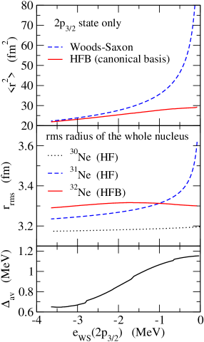
Figure 1: (Color online) (left panel) The mean square radii and the average paring gap as a function of the single particle energy $\varepsilon_{\rm WS}$ in a Woods-Saxon mean-field potential. The top panel shows the mean square radius of the 2s_1/2 wave function with and without the pairing correlation, denoted by HFB and Woods-Saxon, respectively. The middle panel shows the rms radii for ²²O (the dotted line), ²³O (the dashed line), and ²⁴O (the solid line), obtained with the Hartree-Fock (²²O and ²³O) and the Hartree-Fock-Bogoliubov (²⁴O) calculations. The bottom panel shows the results of the HFB calculations for the average paring gap of ²⁴O. (right panel) Same as the left panel, but for the 2$p_{3/2}$ state and for ^30,31,32Ne isotopes.

We now numerically carry out mean-field calculations with a Woods-Saxon (WS) potential and also HFB calculations using the single-particle wave functions in the WS potential. Most of following materials of this section are taken from refs. [14]. As examples of $s$-wave and $p$-wave states, we choose the 2$s_{1/2}$ state in ²³O and 2$p_{3/2}$ state in ³¹Ne, respectively. Although ³¹Ne is most likely a deformed nucleus[22, 23], for simplicity we assume a spherical Woods-Saxon mean-field potential. Notice that a Woods-Saxon potential with a large diffuseness parameter $a$ yields the 2$p_{3/2}$ state which is lower in energy than the 1$f_{7/2}$ state, as was shown in Ref. [24]. We use a similar potential with $a$=0.75 fm as in Ref. [24] for ³¹Ne, while that in Ref. [25] for ²³O. For the HFB calculations, we use the density-dependent contact pairing interaction of surface type, in which the parameters are adjusted in order to reproduce the empirical neutron pairing gap for ³⁰Ne [26]. While we fix the Woods-Saxon potential for the mean-field part, the pairing potential is obtained self-consistently with the contact interaction.

The left top panel of Fig. 1 shows the mean square radius of the 2$s_{1/2}$ state for ²³O, while right top panel of Fig. 1 shows the mean square radius of the 2$p_{3/2}$ state for ³¹Ne. In order to investigate the dependence on the single-particle energy, we vary the depth of the Woods-Saxon wells for the $s_{1/2}$ and $p_{3/2}$ states for ²³O and ³¹Ne, respectively. The dashed lines are obtained with the single-particle wave functions, while the solid lines are obtained with the wave function for the canonical basis in the HFB calculations. One can see an extremely large increase of the radius of the WS wave function for both the $s$-wave and $p$-wave states in the limit of $\epsilon_{\rm WS}\rightarrow 0$. In contrast, the HFB wave functions show only a small increase of radius even in the limit of $\epsilon_{WS}\rightarrow 0$. This feature remains the same even when the contribution of the other orbits are taken into account, as shown in the middle panel of Figs. 1. Due to the pairing effect in the continuum, the HFB calculations yield a larger radius than the HF calculations for the cases of $\epsilon_{\rm WS}\leq-1$ MeV. On the other hand, in the case of $-1$ MeV $<\epsilon_{\rm WS}<0$ MeV the HF wave function (equivalently one quasi-particle wave function in HFB) extends largely, while the HFB wave function does not get much extension due to the pairing anti-halo effect.

In the bottom panel of Figs. 1, the average pairing gaps are shown as a function of the single particle energy $\epsilon_{\rm WS}$. It is seen that the average pairing gap increases as $\epsilon_{\rm WS}$ approaches zero. This is due to the fact that the paring field couples with the extended wave functions of weakly bound nucleons in the self-consistent calculations. That is, the pairing field is extended as the wave functions do and becomes larger for a loosely bound system.

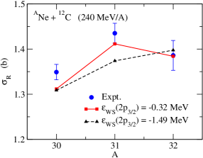
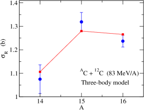
Figure 2: (Color online) (left panel) Reaction cross sections of Ne isotopes on a ¹²C target at $E_{\rm lab}$=240 MeV/A. The cross sections are calculated with the Glauber theory with HF and HFB densities. The solid line with the filled squares shows the results of $S_{n}$(³¹Ne) =$|\varepsilon(2p_{3/2})|$=0.32 MeV, while the dashed line with the open triangles is obtained for $S_{n}$(³¹Ne) =$|\varepsilon(2p_{3/2})|$=1.49 MeV. The experimental data are taken from Ref. [12]. (right panel) Reaction cross sections of C isotopes on a ¹²C target at $E_{\rm lab}$=83 MeV/A. The cross sections are calculated with the Glauber theory with three-body model densities. The experimental data are taken from Ref. [10].

Let us now calculate the reaction cross sections for the ^30,31,32Ne isotopes and discuss the role of pairing anti-halo effect. To this end, we use the Glauber theory, in which we adopt the prescription in Refs. [24, 27] in order to take into account the effect beyond the optical limit approximation. The left panel of Fig. 2 shows the reaction cross sections of the ^30,31,32Ne nuclei on a ¹²C target at 240 MeV/nucleon. We use the target density given in Ref. [28] and the profile function for the nucleon-nucleon scattering given in Ref. [29]. In order to evaluate the phase shift function, we use the two-dimensional Fourier transform technique [30]. The cross sections $\sigma_{R}$ shown in Fig. 2 are calculated by using projectile densities constrained to two different separation energies of the 2$p_{3/2}$ neutron state. The dashed line with triangles is obtained using the wave functions with the separation energy $S_{n}$ (³¹Ne) =$|\epsilon_{\rm WS}|$=1.49 MeV, while the solid line with squares is calculated with the wave functions of $S_{n}$(³¹Ne)=$|\epsilon_{\rm WS}|$=0.32 MeV. The empirical separation energy of ³¹Ne has a large ambiguity with $S_{n}$=0.29$\pm 1.64$ MeV[31]. The cross section $\sigma_{R}$ of ³⁰Ne is already much larger than the systematic values of Ne isotopes with A$<$30. On top of that, we can see a clear odd-even staggering in the results with the smaller separation energy, $S_{n}$=0.32 MeV, as much as in the experimental data, while almost no staggering is seen in the case of the larger separation energy, $S_{n}$=1.49 MeV. This difference is easily understood by looking at the anti-halo effect for $|\epsilon_{\rm WS}|\leq 1$MeV shown in the middle panel of Fig. 1. Recently, the effect of deformation of neutron-rich Ne isotopes on reaction cross sections was evaluated using a deformed Woods-Saxon model [32, 33]. It was shown that the deformation is large as much as $\beta_{2}\sim 0.42$ in ³¹Ne and enhances the reaction cross section by about 5%. However, the calculated results did not show any significant odd-even staggering in $\sigma_{R}$ between ²⁸Ne and ³²Ne [32].

We investigate next neutron-rich C isotopes. We particularly study the ¹⁶C nucleus using a three-body model given in Ref. [34]. In this case, the valence neutron in ¹⁵C occupies the 2$s_{1/2}$ level at $\epsilon_{\rm WS}=-1.21$ MeV, while ¹⁶C is an admixture of mainly the $(2s_{1/2})^{2}$ and $(1d_{5/2})^{2}$ configurations. Assuming the set D given in Ref. [34] for the parameters of the Woods-Saxon and the density distribution for ¹⁴C given in Ref. [35], the rms radii are estimated to be 2.53, 2.90, and 2.81 fm for ¹⁴C, ¹⁵C, and ¹⁶C, respectively. The corresponding reaction cross sections $\sigma_{R}$ calculated with the Glauber theory are shown in the right panel of Fig. 2. The calculation well reproduces the experimental odd-even staggering of the reaction cross sections, that is a clear manifestation of the pairing anti-halo effect.

In order to quantify the OES of reaction cross sections, we introduce the staggering parameter defined by

$$\gamma_{3}=(-)^{A}\frac{\sigma_{R}(A+1)-2\sigma_{R}(A)+\sigma_{R}(A-1)}{2},$$ (43)

where $\sigma_{R}(A)$ is the reaction cross section of a nucleus with mass number $A$. We can define the same quantity also for rms radii. Notice that this staggering parameter is similar to the one often used for the OES of binding energy, that is, the pairing gap.

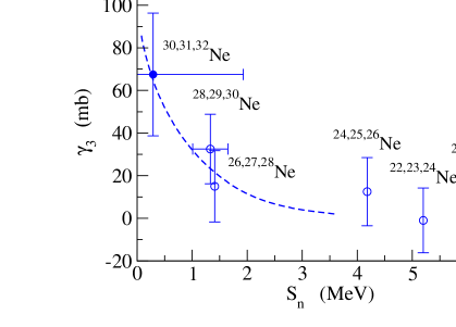
Figure 3: (Color online) The staggering parameter $\gamma_{3}$ of reaction cross sections defined by Eq. (43) for the Ne isotopes with the ¹²C target at $E$=240 MeV/nucleon. This is plotted as a function of the neutron separation energy S_n of the odd-$A$ nuclei. The experimental data for the reaction cross sections are taken from Ref. [12], while the empirical separation energies are taken from Refs. [36, 31]. The dashed line is the calculated staggering parameter for the ^30,31,32Ne isotopes, assuming that the valence neutron of ³¹Ne occupies the 2p${}_{3}/2$ orbit.

The experimental staggering parameters $\gamma_{3}$ are plotted in Fig. 3 for Ne isotopes as a function of the neutron separation energy for the odd-mass nuclei. We use the experimental reaction cross sections given in Ref. [13] while we evaluate the separation energies with the empirical binding energies listed in Ref. [36]. For the neutron separation energy for the ³¹Ne nucleus, we use the value in Ref. [31]. The experimental uncertainties of the staggering parameter are obtained as

$$\delta\gamma_{3}=\frac{\sqrt{(\delta\sigma_{R}(A+1))^{2}+4(\delta\sigma_{R}(A))^{2}+(\delta\sigma_{R}(A-1))^{2}}}{2},$$ (44)

where $\delta\sigma_{R}(A)$ is the experimental uncertainty for the reaction cross section of a nucleus with mass number $A$. The figure also shows by the dashed line the calculated staggering parameter for the ^30,31,32Ne nuclei with the 2p_3/2 orbit. One sees that the experimental staggering parameter agrees with the calculated value for ^30,31,32Ne nuclei when one assumes that the valence neutron in ³¹Ne occupies the 2p_3/2 orbit. Furthermore, although the structure of lighter odd-A Ne isotopes is not known well, it is interesting to see that the empirical staggering parameters closely follow the calculated values for the 2p_3/2 orbit. This may indicate that the low-$l$ single-particle orbits are appreciably mixed in these Ne isotopes due to the deformation effects[22, 23].

4 Isospin Dependent Pairing Interaction and Pairing Gaps in Finite Nuclei

There are mainly two different approaches for a calculation of pairing correlations in finite nuclei. The first approach is based on phenomenological pairing interactions whose parameters are determined using some selected data [37], while the second approach starts from a bare nucleon-nucleon interaction and eventually includes the effect of phonon coupling [38]. The latter approach has shown that the medium polarization reduces the pairing gaps in neutron matter while, in symmetric matter, the neutron pairing gaps are much enlarged at low density compared to that of the bare calculation. This enhancement takes place especially for neutron Fermi momenta $k_{\mathrm{Fn}}<0.7$ fm^-1.

We propose effective density-dependent pairing interactions which reproduce both the neutron-neutron ($nn$) scattering length at zero density and the neutron pairing gap in uniform matter. In order to simultaneously describe the density dependence of the neutron pairing gap for both symmetric and neutron matter, it is necessary to include an isospin dependence in the effective pairing interaction [9]. Depending on whether the medium polarization effects on the pairing gap given in Ref. [39] are taken into account or not, we invent two different density dependent functionals in the pairing interaction. Then, we apply these interactions to study pairing gaps in semi-magic finite nuclei, such as Ca, Ni, Sn and Pb isotopic chains.

The density$-$dependent pairing interaction can be read as

$$v_{\rm pair}(1,2)=\frac{1-\mathrm{P}_{\sigma}}{2}v_{0}\,\mathrm{g}[\rho,I]\,\delta(\vec{\rm r}_{1}-\vec{\rm r}_{2}).$$ (45)

where $\rho$ is the nuclear density and $I$ is defined as $I=(\rho_{n}-\rho_{p})/\rho\cdot\tau_{z}$ [9]. In Ref. [9], an isovector dependence in the density-dependent term $\mathrm{g}$ is separated to two parts $\mathrm{g}=\mathrm{g}^{1}+\mathrm{g}^{2}$. The function $\mathrm{g}^{1}$ is determined to mimic the bare pairing gaps in nuclear matters and the function $\mathrm{g}^{2}$ takes care of the medium polarization effect. The functional form of $\mathrm{g}^{1}$ is given by

$$\mathrm{g}^{1}[\rho,I]=1-\mathrm{f}_{\mathrm{s}}(I)\eta_{\mathrm{s}}\left(\frac{\rho}{\rho_{0}}\right)^{\alpha_{\mathrm{s}}}-\mathrm{f}_{\mathrm{n}}(I)\eta_{\mathrm{n}}\left(\frac{\rho}{\rho_{0}}\right)^{\alpha_{\mathrm{n}}}\;,$$ (46)

where $\rho_{0}$=0.16 fm^-3 is the saturation density of symmetric nuclear matter and the functions $\mathrm{f}_{\mathrm{s}}(I)$ and $\mathrm{f}_{\mathrm{n}}(I)$ are $\mathrm{f}_{\mathrm{s}}(I)=1-\mathrm{f}_{\mathrm{n}}(I)$ and $\mathrm{f}_{\mathrm{n}}(I)=I=(\rho_{\mathrm{n}}(r)-\rho_{\mathrm{p}}(r))/\rho(r)\cdot\tau_{z}$. The values of parameters $\eta_{\mathrm{s}},\eta_{\mathrm{n}}$ and powers of density dependence $\alpha_{\mathrm{s}},\alpha_{\mathrm{n}}$ are given elsewhere [9].

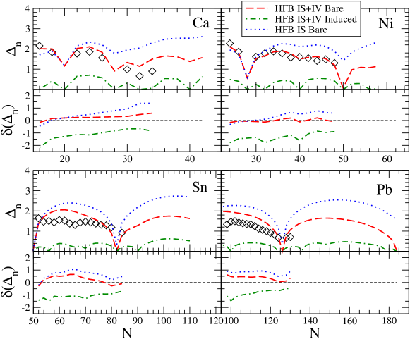
Figure 4: Comparison of the neutron HFB pairing gaps $\Delta_{\mathrm{n}}$ with the odd-even mass staggering given by the three-point formula $\Delta^{(3)}$. The dotted line shows the results of the pairing interactions IS+IV Bare, while the short dashed, and long dashed lines are obtained with the pairing interactions IS+IV Screened and IS Bare, respectively. The difference $\delta(\Delta_{\mathrm{n}})$ is defined as $\delta(\Delta_{\mathrm{n}})=\Delta_{\mathrm{n}}(\mathrm{th.})-\Delta_{\mathrm{n}}(\mathrm{exp.})$. All units are given in MeV.

We perform Hartree-Fock-Bogoliubov (HFB) calculations for semi-magic Calcium, Nickel, Tin and Lead isotopes using these density-dependent pairing interactions in Eq. (45) derived from a microscopic nucleon-nucleon interaction. Our calculations reproduce well the neutron number dependence of experimental data for binding energy, two neutrons separation energy, and odd-even mass staggering of these isotopes [40]. Especially the interaction IS+IV Bare without the medium polarization effect gives satisfactory results of all the isotopes as is seen in Fig. 4. It is clear in the comparison between IS bare and IS+IV bare that the isospin dependence of the pairing interaction plays an important role in the pairing gaps of neutron-rich nuclei. The isospin dependent pairing interaction is further applied to both even-even and even-odd nuclei by using EV8-odd program. The results successfully reproduce the empirical isotope and isotone dependent functionals of the odd-even mass differences of several medium-heavy and heavy nuclei [41]. Yamagami et al., studied also the quadratic isospin dependent terms of pairing interaction [42, 43]. They adopted several Skyrme interactions with different effective mass and showed the effective mass dependence of the isospin dependent terms. It is also shown in ref. [44] that the effect of Coulomb two-body interaction on the proton pairing gaps can be mimicked by the leaner isospin dependent term in the pairing interaction.

5 Summary

We have studied the mass radii of Ne isotopes with the Hartree-Fock (HF) and Hartree-Fock-Bogoliubov (HFB) methods with a Woods-Saxon potential. The reaction cross sections $\sigma_{R}$ were calculated using the Glauber theory with these microscopic densities. We have shown that the empirical odd-even staggering in the reaction cross sections of neutron-rich Ne isotopes with the mass A=$30\sim 32$ is well described by the HFB density and can be considered as a clear manifestation of the pairing anti-halo effect associated with a loosely-bound 2$p_{3/2}$ wave function. The index of the odd-even staggering is proposed and applied successfully for the study of the reaction cross sections of Ne isotopes to revel the role of the pairing correlations in exotic nuclei.

A new type of density dependent contact pairing interaction was obtained to reproduce the microscopic pairing gaps in symmetric and neutron matter. We performed also HFB calculations for semi-magic Calcium, Nickel, Tin and Lead isotopes using these density-dependent pairing interactions. Our calculations reproduce well the neutron number dependence of experimental data of binding energy, two neutrons separation energy, and odd-even mass staggering of these isotopes with the interaction IS+IV Bare. Recently, the isospin dependent interaction is extended to introduce the quadratic terms of isospin and applied to a wide region of nuclei in the mass table. These result suggests that by introducing the isospin dependent term in the pairing interaction, one can construct a global effective pairing interaction which is applicable to nuclei in a wide range of the nuclear chart.

References

References

- [1] A. Bohr, B. R. Mottelson, and D. Pines, Phys. Rev. 110, 936 (1958).
- [2] A. Bohr and B. R. Mottelson, Nuclear Structure(Benjamin, New York, 1969) Vol. I.
- [3] D. M. Brink and R. Broglia, “Nuclear superfluidity, pairing in Finite Systems”, Cambridge monographs on particle physics, nuclear physics and cosmology, vol 24 (2005).
- [4] G. F. Bertsch, “ 50 Years of Nuclear BCS”, (World Scientific, edited by R. Broglia and V. Zelevinsky), arXiv:1203.5529v1 (March,2012).
- [5] K. Matsuyanagi, N. Hinohara, and K. Sato, arXiv:1205.0078v1 (May,2012).
- [6] M. Bender, P.-H.Heenen and P.-G. Reinhard, Rev. Mod. Phys. 75, 121 (2003).
- [7] M. V. Stoitsov, J. Dobaczewski, W. Nazarewicz and P. Borycki, Int. J. Mass Spectrum, 251, 243 (2006).
- [8] T. Duguet, P. Bonche, P.-H. Heenen, and J. Meyer, Phys. Rev. C 65, 014311 (2001).
- [9] J. Margueron, H. Sagawa and K. Hagino, Phys. Rev. C 76, 064316 (2007); Phys. Rev. C 77, 054309 (2008).
- [10] D.Q. Fang et al., Phys. Rev. C69, 034613 (2004).
- [11] A. Ozawa et al., Nucl. Phys. A691, 599 (2001).
- [12] M. Takechi et al., Nucl. Phys. A834, 412c(2010), and private communication.
- [13] M. Takechi et al., private communication.
- [14] K. Hagino and H. Sagawa, Phys. Rev. C84, 011303(R) (2011); Phys. Rev. C85, 014303(2012) ; Phys. Rev. C85, 037604(2012)
- [15] K. Bennaceur, J. Dobaczewski and M. Ploszajczak, Phys. Lett. B496, 154 (2000).
- [16] P. Schuck and X. Vinas, Phys. Rev. Lett. 107, 205301 (2011).
- [17] A. Bulgac, arXiv:nucl-th/9907088.
- [18] K. Hagino and H. Sagawa, Phys. Rev. C 71 044302 (2005).
- [19] K. Riisager, A.S. Jensen and P. Moller, Nucl. Phys. A548, 393 (1992).
- [20] H. Sagawa, Phys. Lett. B286, 7 (1992).
- [21] J. Dobaczewski et al., Phys. Rev. C53, 2809 (1996).
- [22] I. Hamamoto, Phys. Rev. C81, 021304(R) (2010).
- [23] Y. Urata, K. Hagino, and H. Sagawa, Phys. Rev. C83, 041303(R) (2011).
- [24] W. Horiuchi, Y. Suzuki, P. Capel, and D. Baye, Phys. Rev. C81, 024606 (2010).
- [25] K. Hagino and H. Sagawa, Phys. Rev. C72, 044321 (2005).
- [26] M. Yamagami and Nguyen Van Giai, Phys. Rev. C69, 034301 (2004).
- [27] B. Abu-Ibrahim and Y. Suzuki, Phys. Rev. C62, 034608 (2000).
- [28] Y. Ogawa, K. Yabana, and Y. Suzuki, Nucl. Phys. A543, 722 (1992).
- [29] B. Abu-Ibrahim et al., Phys. Rev. C77, 034607 (2008).
- [30] C.A. Bertulani and H. Sagawa, Nucl. Phys. A588, 667 (1995).
- [31] B. Jurado et al., Phys. Lett. B649, 43 (2007).
- [32] K. Minomo et al., Phys. Rev. C8̱4, 034602 (2011); Phys. Rev. Lett. 108, 052503 (2012).
- [33] Y. Urata, K. Hagino, and H. Sagawa, Phys. Rev. C86, 044613(2012).
- [34] K. Hagino and H. Sagawa, Phys. Rev. C75, 021301(R) (2007).
- [35] Yu. L. Parfenova, M.V. Zhukov, and J.S. Vaagen, Phys. Rev. C62, 044602 (2000).
- [36] G. Audi and A.H. Wapstra, Nucl. Phys. A595, 409 (1995).
- [37] J. Dobaczewski, W. Nazarewicz, and P.-G. Reinhard, Nucl. Phys. A693, 361 (2001).
- [38] F. Barranco et al, Phys. Rev. Lett. 83, 2147 (1999).
- [39] L. G. Cao, U. Lombardo, and P. Schuck, Phys. Rev. C 74, 064301 (2006).
- [40] J. Margueron, H. Sagawa, and K. Hagino, Phys. Rev. C 77, 054309 (2008).
- [41] C. A. Bertulani, H. F. Lu and H. Sagawa, Phys. Rev. C80, 027303(2009).
- [42] M. Yamagami, Y. R. Shimizu and T. Nakatsukasa, Phys. Rev. C 80, 064301 (2009).
- [43] M. Yamagami, J. Margueron, H. Sagawa and K. Hagino, Phys. Rev. C86, 034333 (2012).
- [44] H. Nakada and M. Yamagami, Phys. Rev. C83, 031302 (2011).