Supersolid in Bose-Bose-Fermi Mixtures subjected to a Square Lattice

Abstract

Two-component Bose condensates with repulsive interaction are stable when $g_{\rm\scriptscriptstyle 1}g_{\rm\scriptscriptstyle 2}<g_{\rm\scriptscriptstyle 12}^{2}$ is satisfied. By tuning the interactions, we show that the instability corresponding to bose-bose phase separation always happens at a higher temperature than corresponding to bose-fermi phase separation happens. Moreover, we find both the transition temperature $T_{\rm\scriptscriptstyle DW}$ of supersolid and the coherence peak at $k_{\rm\scriptscriptstyle DW}$ are enhanced in the mixtures studied. These will make the observation of supersolid in experiments more reachable.

I Introduction

Supersolids, a concept simultaneously exhibiting superfluidity and crystalline order, have been studied intensely over five decades O. Penrose ; A. F. Andreev ; G. V. Chester ; A. J. Leggett . Theoretically, people mainly focus on lattice models of interacting bosons and fermions such as the Hubbard model and its various generalizations and have obtained many important results by numerical analysis G. G. Batrouni ; I. Titvinidze . Experimentally, Kim and Chan recently reported they found nonclassical rotational inertia which should be an direct evidence of supersolid based on Leggett’s suggestion in solid ⁴He E. Kim1 ; E. Kim2 , however, it has also been pointed out that this observation may not be due to supersolid but due to other reasons, such as an increase in shear modulus of bulk solid helium J. Day , and triggered an intense debate M. Boninsegni ; D. Y. Kim .

Besides the study of supersolids in condensed matter systems, ultracold atoms in optical lattices D. Jaksch have emerged as a parallel platform with highly controllability to study supersolids. Trapped Bose-Einstein condensates with dipole-dipole interaction can produce a “roton” minimum in the excitation spectrum D. H. J. O'Dell ; L. Santos ; Shai Ronen , and this led to the prediction of supersolid upon softening of the roton excitation energy D. Kirzhnits ; G. Blatter . Recently, on the basis of off-resonant dressing of atomic Bose-Einstein condensates to high-lying Rydberg states, people have found the effective atomic interactions resulting from such a Rydberg dressing can also produce a roton minimum and, therefore, provide a clean realization of available model for supersolidity N. Henkel ; F. Cinti .

In this work, we consider the two kind of bosons are two hyperfine state of ⁸⁷Rb, and the fermions are a hyperfine state of ⁴⁰K and investigate bose-bose-fermi mixtures in a square lattice. For the bose-fermi mixtures subjected to a square lattice, it has been pointed out that the density wave instability introduced by fermions will establish crystalline order, while the condensate bosons exhibit superfluidity, so a supersolid phase emerges at finite temperature G. Blatter . For the bose-bose-fermi mixtures studied here, besides the density wave instability introduced by fermions, there is another instability between the two-component bose-condensates when $g_{\rm\scriptscriptstyle 1}g_{\rm\scriptscriptstyle 2}=g_{\rm\scriptscriptstyle 12}^{2}$, where $g_{\rm\scriptscriptstyle 1,2}$ are the repulsive intraspecies interaction and $g_{\rm\scriptscriptstyle 12}$ is the interspecies interaction E. Timmermans . When $g_{\rm\scriptscriptstyle 1}g_{\rm\scriptscriptstyle 2}>g_{\rm\scriptscriptstyle 12}^{2}$, the bose-condensates are mixed and stable. When $g_{\rm\scriptscriptstyle 1}g_{\rm\scriptscriptstyle 2}<g_{\rm\scriptscriptstyle 12}^{2}$, the bose-condensates are unstable and tend to either phase separation or collapse depending on $g_{\rm\scriptscriptstyle 12}>0$ or $<0$. In this article, we assume the bose-condensates are initially mixed and stable, and we find that bose-bose phase separation always happens before bose-fermi phase separation when we decrease the temperature. Moreover, we find both the transition temperature $T_{\rm\scriptscriptstyle DW}$ of supersolid and the coherence peak at $k_{\rm\scriptscriptstyle DW}$ are enhanced comparing to the bose-fermi mixtures case G. Blatter .

The article is organized as follows. In Sec.II, we consider the two kind of bosons are two hyperfine state of ⁸⁷Rb, and the fermions are a hyperfine state of ⁴⁰K and investigate bose-bose-fermi mixtures in a square lattice, and give the fermionic response in the static limit. In Sec.III, we give the details of the instabilities and different phases induced by the instabilities, and give a mean field description of the supersolid phase. Some conclusions are obtained in Sec.IV.

II The bose-bose-fermi mixtures in a square lattice

The Hamiltonian for the bose-bose-fermi mixtures takes the form $H=H_{0}+H_{int}$ with ($\alpha=\uparrow,0,\downarrow$)

$$H_{0} = \sum_{\alpha}\int d{\bf x}\psi_{\alpha}^{{\dagger}}\left\{(-\frac{\hbar^{2}}{2m_{\alpha}}\bigtriangledown^{2}+V_{\alpha}(x)\right\}\psi_{\alpha},$$

$$H_{int} = \int d{\bf x}\left\{g_{\rm\scriptscriptstyle 1}\psi_{\uparrow}^{{\dagger}}\psi_{\uparrow}^{{\dagger}}\psi_{\uparrow}\psi_{\uparrow}+g_{\rm\scriptscriptstyle 2}\psi_{\downarrow}^{{\dagger}}\psi_{\downarrow}^{{\dagger}}\psi_{\downarrow}\psi_{\downarrow}\right.$$

$$\left.+2g_{\rm\scriptscriptstyle 12}\psi_{\uparrow}^{{\dagger}}\psi_{\downarrow}^{{\dagger}}\psi_{\downarrow}\psi_{\uparrow}+2g_{\rm\scriptscriptstyle BF}\left(\psi_{\uparrow}^{{\dagger}}\psi_{\uparrow}+\psi_{\downarrow}^{{\dagger}}\psi_{\downarrow}\right)\psi_{0}^{{\dagger}}\psi_{0}\right\},$$

where $\psi^{{\dagger}}_{\uparrow,\downarrow}$ are the bosonic field operators and $\psi^{{\dagger}}_{0}$ is the fermionic field operator. In order to assure the mixtures to be stable, we assume all of the interactions between bosons are repulsive, with $g_{\alpha\beta}=4\pi a_{s,\alpha\beta}\hbar^{2}/m$ ($\alpha,\beta=1,2$. In this work, we use $\alpha,\beta$ to label the interactions, densities and phases of bosons, and use $\uparrow,\downarrow$ only to label the bosonic operators, moreover, when $\alpha=\beta$ we only keep $\alpha$ for convenience) and $g_{\rm\scriptscriptstyle 1}g_{\rm\scriptscriptstyle 2}>g_{\rm\scriptscriptstyle 12}^{2}$. $g_{\rm\scriptscriptstyle BF}=2\pi a_{\rm\scriptscriptstyle BF}\hbar^{2}/\mu$, the strength of coupling between bosons and fermions, we assume that they are equal for both component of bosons. $a_{s,\alpha}$ is the intraspecies scattering length, $a_{s,12}$ is the interspecies scattering length, and $\mu$ is the relative mass. $V_{\alpha}({\bf x})=V_{\alpha}[\sin^{2}(\pi x/a)+\sin^{2}(\pi y/a)]$ is the periodic potential produced by the optical lattice with wave-length $\lambda=2a$ and $m_{\alpha}$ are the mass of bosons and fermions. As the bosons are two hyperfine state of ⁸⁷Rb, it is justified to assume $m_{\uparrow}=m_{\downarrow}$ and $V_{\uparrow}=V_{\downarrow}$ for simplicity in the following. Since the fermions are single component, the interaction between them can be neglected due to Pauli exclusion principle.

In order to obtain the Hamiltonian in momentum space, we follow the procedures used in Ref.G. Blatter and expand the bosonic and fermionic field operators $\psi_{\alpha}$ in the forms

$$\psi_{\uparrow,\downarrow}(x) = \sum_{{\bf k}\in K}b_{{\bf k}\uparrow,\downarrow}w_{{\bf k}\uparrow,\downarrow}(x),$$

$$\psi_{0}(x) = \sum_{{\bf k}\in K}c_{{\bf k}}v_{{\bf k}}(x),$$ (2)

where $K$ denotes the first Brillouin zone, $b_{{\bf k}\uparrow,\downarrow}$ and $c_{{\bf k}}$ are the bosonic and fermionic annihilation operators, while $w_{{\bf k}\uparrow,\downarrow}(x)$ and $v_{{\bf k}}(x)$ are the Bloch wave functions corresponding to a single boson ($\uparrow$ or $\downarrow$) or fermion in the periodic potential $V_{\alpha}$, respectively. Since $m_{\uparrow}=m_{\downarrow}$ and $V_{\uparrow}=V_{\downarrow}$, $w_{{\bf k}\uparrow}(x)$ should be equal to $w_{{\bf k}\downarrow}(x)$. Therefore, we use $w_{{\bf k}}(x)$ to denote both of them for convenience. Substituting Eq.(2) into Eq.(II) and restricting in the lowest Bloch band, we obtain the Hamiltonian in momentum space as

$$H = \sum_{{\bf k}\in K,\sigma}\epsilon_{\rm\scriptscriptstyle B\sigma}b_{{\bf k}\sigma}^{{\dagger}}b_{{\bf k}\sigma}+\sum_{\{{\bf k,k^{\prime},q,q^{\prime},\sigma}\}}\frac{U_{\scriptscriptstyle\rm B\sigma}}{2N}b^{+}_{{\bf k}\sigma}b_{{\bf k}^{\prime}\sigma}b^{+}_{{\bf q}\sigma}b_{{\bf q}^{\prime}\sigma}$$ (3)

$$+\sum_{\{{\bf k,k^{\prime},q,q^{\prime}}\}}\frac{U_{\scriptscriptstyle\rm B,12}}{N}b^{+}_{{\bf k}\uparrow}b_{{\bf k}^{\prime}\uparrow}b^{+}_{{\bf q}\downarrow}b_{{\bf q}^{\prime}\downarrow}+\sum_{{\bf q}\in K}\epsilon_{\scriptscriptstyle\rm F}({\bf q})c^{+}_{{\bf q}}c_{{\bf q}}$$

$$+\frac{U_{\scriptscriptstyle\rm BF}}{N}\sum_{\{{\bf k,k^{\prime},q,q^{\prime},\sigma}\}}b^{+}_{{\bf k}\sigma}b_{{\bf k}^{\prime}\sigma}c^{+}_{{\bf q}}c_{{\bf q}^{\prime}},$$

where $N$ is the number of unit cells, $\epsilon_{\scriptscriptstyle\rm F,B\sigma}({\bf k})$ denote the energy dispersion of the fermions and bosons, respectively, while $U_{\scriptscriptstyle\rm BF}=g_{\scriptscriptstyle\rm BF}\int d{\bf x}|\widetilde{w}|^{2}|\widetilde{v}|^{2}$ and $U_{\scriptscriptstyle\rm B,\alpha\beta}=g_{\scriptscriptstyle\rm\alpha\beta}\int d{\bf x}|\widetilde{w}|^{4}$, with $\widetilde{w}({\bf x})$ and $\widetilde{v}({\bf x})$, the Wannier functions associated with the Bloch band $w_{{\bf k}}({\bf x})$ and $v_{{\bf k}}({\bf x})$. In a deep optical lattice, the Wannier functions $\widetilde{w}({\bf x})$ and $\widetilde{v}({\bf x})$ are well localized around the minimum of $V_{\alpha}$. As a result, the Hamiltonian reduces to a familiar Bose-Fermi-Hubbard model, and for $\epsilon_{\scriptscriptstyle\rm F,B\sigma}({\bf k})$, only nearest neighbor hopping survives,

$$\epsilon_{\scriptscriptstyle\rm B}({\bf q}) = 2J_{\rm\scriptscriptstyle B}\left[2-\cos\left(q_{x}a\right)-\cos\left(q_{y}a\right)\right],$$

$$\epsilon_{\scriptscriptstyle\rm F}({\bf q}) = -2J_{\rm\scriptscriptstyle F}\left[\cos\left(q_{x}a\right)+\cos\left(q_{y}a\right)\right],$$ (4)

where $J_{\rm\scriptscriptstyle B,F}$ is the hopping energy for fermions and bosons, respectively. The bosonic dispersion relation implies $\mu_{B}=-4J_{B}$ and the bosons will form a zero-momentum Bose-Einstein condensation for sufficiently low temperature. The fermionic dispersion relation implies the Fermi surface at half-filling $n_{\rm\scriptscriptstyle F}=1/2$ (where $\mu_{\rm F}=0$, in this work. $n_{\rm\scriptscriptstyle F}$ and $n_{\rm\scriptscriptstyle B}$ denote the number of particles per unit cell) and exhibits perfect nesting for ${\bf k}_{\rm\scriptscriptstyle DW}=(\pi/a,\pi/a)$ and van Hove singularities at ${\bf k}=(0,\pm\pi/a),(\pm\pi/a,0)$.

Integrating out the fermions produces two effects. To the first order in $U_{\scriptscriptstyle\rm BF}$ (in this work, we focus on weak interaction, so an expansion in $U_{\scriptscriptstyle\rm BF}$ and a cut at the second order are justified), the fermions simply produce a (trivial) shift of the bosonic chemical potential $\mu_{\scriptscriptstyle\rm B\sigma}\rightarrow\mu_{\scriptscriptstyle\rm B\sigma}-U_{\scriptscriptstyle\rm BF}n_{\scriptscriptstyle\rm F}$. To the second order in $U_{\scriptscriptstyle\rm BF}$, the fermions provide an effective interaction for the bosons which depends on the temperature $T$ of the fermionic atom gas,

$$H_{\rm\scriptscriptstyle int} = \frac{1}{2N}\sum_{\{{\bf k,k^{\prime},q,q^{\prime},\sigma}\}}U_{\rm\scriptscriptstyle B\sigma}(T,{\bf q-q^{\prime}})b^{+}_{{\bf k}\sigma}b_{{\bf k}^{\prime}\sigma}b^{+}_{{\bf q}\sigma}b_{{\bf q}^{\prime}\sigma}$$

$$+\frac{1}{N}\sum_{\{{\bf k,k^{\prime},q,q^{\prime},}\}}U_{\rm\scriptscriptstyle B,12}(T,{\bf q-q^{\prime}})b^{+}_{{\bf k}\uparrow}b_{{\bf k}^{\prime}\uparrow}b^{+}_{{\bf q}\downarrow}b_{{\bf q}^{\prime}\downarrow},$$

with

$$U_{\rm\scriptscriptstyle B\sigma}(T,{\bf q-q^{\prime}}) = U_{\rm\scriptscriptstyle B\sigma}+U_{\rm\scriptscriptstyle FB}^{2}\chi(T,{\bf q-q^{\prime}}),$$

$$U_{\rm\scriptscriptstyle B,12}(T,{\bf q-q^{\prime}}) = U_{\rm\scriptscriptstyle B,12}+U_{\rm\scriptscriptstyle FB}^{2}\chi(T,{\bf q-q^{\prime}}).$$ (5)

The fermionic response in the static limit is given by the Lindhard function

$$\chi(T,{\bf q})=\int_{K}\frac{d{\bf k}}{v_{0}}\frac{f[\epsilon_{\rm\scriptscriptstyle F}({\bf k})]-f[\epsilon_{\rm\scriptscriptstyle F}({\bf k+q})]}{\epsilon_{\rm\scriptscriptstyle F}({\bf k})-\epsilon_{\rm\scriptscriptstyle F}({\bf k+q})+i\eta},$$ (6)

where $v_{0}=(2\pi/a)^{2}$ is the volume of the first Brillouin zone, $f(\epsilon)=1/[1+\exp(\epsilon/T)]$ ($\mu_{\rm\scriptscriptstyle F}=0$ at half filling) is just the Dirac-Fermi distribution function. The static limit is justified if the fermions are much faster than the bosons ($J_{\rm\scriptscriptstyle F}>>J_{\rm\scriptscriptstyle B}$), as then the fermionic response occurs on much faster timescales than the movement of the bosons, and one can safely neglect retardation effects Peter P. Orth . Using the fermionic dispersion relation Eq.(4), the Lindhard function exhibits two logarithmic singularities at ${\bf q}=0$ and ${\bf k}_{\rm\scriptscriptstyle DW}$. The singularity at ${\bf q}=0$ is purely due to the logarithmic van Hove singularity in the density of states, and the singularity at ${\bf k}_{\rm\scriptscriptstyle DW}$ is due to the combination of van Hove singularities and perfect nesting. The singularity at ${\bf q}=0$ induces an instability towards a series of phase separation, while the singularity at ${\bf k}_{\rm\scriptscriptstyle DW}$ induces an instability towards density wave formation and provides a supersolid phase. The two instabilities are competing with each other.

III INSTABILITIES AND PHASES

For the weak interaction, when the temperatures is well below the superfluid transition temperature $T_{\rm\scriptscriptstyle KT}$ of the bosons, the Lindhard function at ${\bf q}=0$ reduces to $\chi(T\rightarrow 0,0)$ and takes the form G. Blatter

$$\chi(T\rightarrow 0,0)=\int d\epsilon N(\epsilon)\partial_{\epsilon}f(\epsilon)\sim-N_{0}\ln\frac{16c_{1}J_{\rm\scriptscriptstyle F}}{T},$$ (7)

with $N(\epsilon)\sim N_{0}\ln|16J_{\rm\scriptscriptstyle F}/\epsilon|$, $N_{0}=1/(2\pi^{2}J_{\rm\scriptscriptstyle F})$ and $c_{1}=2\exp(C)/\pi\approx 1.13$. As $\chi(T\rightarrow 0,0)$ is always negative, the coupling between the bosons and the fermions induces an attractive interaction, which is proportional to $U_{\rm\scriptscriptstyle FB}^{2}\chi(T,{\bf 0})$, between the bosons (see Eq.(5)). This attractive interaction has the effect to reduce the repulsive interactions $U_{B,\alpha\beta}$ between bosons to $U_{\rm\scriptscriptstyle eff,\alpha\beta}=U_{\rm\scriptscriptstyle B,\alpha\beta}+U_{\rm\scriptscriptstyle FB}^{2}\chi(T,0)$. As a result, even $U_{\rm\scriptscriptstyle B,1}U_{\rm\scriptscriptstyle B,2}>U_{\rm\scriptscriptstyle B,12}^{2}$ (equivalent to $g_{\rm\scriptscriptstyle 1}g_{\rm\scriptscriptstyle 2}>g_{\rm\scriptscriptstyle 12}^{2}$) initially, $U_{\rm\scriptscriptstyle eff,1}U_{\rm\scriptscriptstyle eff,2}$ can be tuned to equal to $U_{\rm\scriptscriptstyle eff,12}^{2}$ by lowering the temperature to some value. Moreover, a superfluid condensate at low temperatures to be stable requires a positive effective interaction $U_{\rm\scriptscriptstyle eff,\alpha}>0$. If we take $U_{\rm\scriptscriptstyle B,1}$ as the energy unit, and define the ratios $U_{\rm\scriptscriptstyle B,2}/U_{\rm\scriptscriptstyle B,1}$, $U_{\rm\scriptscriptstyle B,12}/U_{\rm\scriptscriptstyle B,1}$ and $U_{\rm\scriptscriptstyle BF}/U_{\rm\scriptscriptstyle B,1}$ as $\gamma$, $\lambda$ and $\kappa$, respectively. The condition $U_{eff,12}^{2}=U_{eff,1}U_{eff,2}$ defines the critical temperature $T_{\rm\scriptscriptstyle BB,PS}$ for bose-bose phase separation,

$$T_{\rm\scriptscriptstyle BB,PS}=16c_{1}J_{\rm\scriptscriptstyle F}\exp\left[\frac{\lambda^{2}-\gamma}{N_{0}\kappa^{2}(1+\gamma-2\lambda)}\right].$$ (8)

The condition $U_{\rm\scriptscriptstyle eff,\alpha}=0$ defines two critical temperatures $T_{\rm\scriptscriptstyle BF1,PS}$ and $T_{\rm\scriptscriptstyle BF2,PS}$ for bose-fermi phase separation.

$$T_{\rm\scriptscriptstyle BF1,PS} = 16c_{1}J_{\rm\scriptscriptstyle F}\exp\left[-\frac{1}{N_{0}\kappa^{2}}\right],$$

$$T_{\rm\scriptscriptstyle BF2,PS} = 16c_{1}J_{\rm\scriptscriptstyle F}\exp\left[-\frac{\gamma}{N_{0}\kappa^{2}}\right].$$ (9)

When $\lambda\neq 1$ and $\gamma$, it is directly to show that $(\gamma-\lambda^{2})/(1+\gamma-2\lambda)$ is always smaller than $\min\{1,\gamma\}$ under the constraint $\lambda^{2}<\gamma$, which is the condition that the bose condensates are initially mixed (see Fig.1). $(\gamma-\lambda^{2})/(1+\gamma-2\lambda)<\min\{1,\gamma\}$ indicates when we lower the temperature, the bose-bose mixtures are always easier to be unstable and phase separated (or collapse, see Fig.1) than the bose-fermi mixtures. Moreover, when $\lambda$ gets close to the boundary $\sqrt{\gamma}$, $(\gamma-\lambda^{2})/(1+\gamma-2\lambda)$ decreases very fast, as a result, $T_{\rm\scriptscriptstyle BB,PS}$ increases exponentially to values much larger than $max\{T_{\rm\scriptscriptstyle BF1,PS},T_{\rm\scriptscriptstyle BF2,PS}\}$ and easy to reach in experiments. Therefore, such a bose-bose phase separation induced by fermions should be easy to be observed in experiments. If we continue to lower the temperature after the bose-bose mixtures are phase separated, we can expect that bose-fermi phase separation will happen and all the components will distribute separately in space at last.

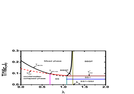
Figure 1: (Color online) $\lambda-T$ Phase diagram. Parameters are set as $t_{\rm B}=0.55$, $N_{0}\kappa^{2}=0.39$, $\gamma=1.5$, $\lambda_{c}=\sqrt{\gamma}$. For $\lambda>\lambda_{c}$, the two-component bosons are phase separation initially (BBPS), and supersolid corresponding to bosons-$\uparrow$ (SS1) emerges when the temperature is below $T^{\prime}_{DW}$. For $\lambda<\lambda_{c}$, the supersolid phase established by the two Bose-condensates appears when the temperature is below $T_{\rm DW}$ with $T_{\rm BB,PS}<T_{\rm DW}$. For $\lambda<1$ ($1<\lambda<\lambda_{c}$), the two Bose-condensates collapse (separate) when the temperature is below $T_{\rm BB,PS}$ with $T_{\rm BB,PS}>T_{\rm DW}$.

Now, we discuss the second instability induced by the singularity in the Lindhard function at ${\bf k}_{\rm\scriptscriptstyle DW}$. Using Eq.(6) and the perfect nesting $\epsilon_{\scriptscriptstyle\rm F}({\bf q}+{\bf k}_{\rm\scriptscriptstyle DW})\!=-\epsilon_{\scriptscriptstyle\rm F}({\bf q})$, the Lindhard function becomes G. Blatter

$$\chi(T,{\bf k}_{\rm DW})=\int d\epsilon N(\epsilon)\frac{\tanh\left({\epsilon}/{2T}\right)}{-2\epsilon}\sim-\frac{N_{0}}{2}\left[\ln\frac{16c_{1}J_{\rm\scriptscriptstyle F}}{T}\right]^{2}.$$

The combination of van Hove singularities and perfect nesting produces a $[\ln T]^{2}$ singular behavior. Such a singular behavior can produce a roton minimum at ${\bf k}_{\rm\scriptscriptstyle DW}$. Within Bogoliubov theory, the bosonic quasi-particle spectrum becomes

$$E_{\rm\scriptscriptstyle B,\pm}^{2}({\bf q}) = \epsilon_{\rm\scriptscriptstyle B}^{2}({\bf q})+\epsilon_{\rm\scriptscriptstyle B}({\bf q})n_{\rm\scriptscriptstyle B}\left[U_{\rm\scriptscriptstyle B1}(T,q)+U_{\rm\scriptscriptstyle B2}(T,q)\right]$$ (11)

$$\pm\left\{\epsilon_{\rm\scriptscriptstyle B}^{2}({\bf q})n_{\rm\scriptscriptstyle B}^{2}\left[U_{\rm\scriptscriptstyle B1}(T,q)-U_{\rm\scriptscriptstyle B2}(T,q)\right]^{2}\right.$$

$$+\left.4\epsilon_{\rm\scriptscriptstyle B}^{2}({\bf q})n_{\rm\scriptscriptstyle B}^{2}U_{\rm\scriptscriptstyle B,12}^{2}(T,q)\right\}^{1/2},$$

here we have assumed $n_{\rm\scriptscriptstyle B1}=n_{\rm\scriptscriptstyle B2}=n_{\rm\scriptscriptstyle B}$. The induced attraction proportional to $U_{\rm\scriptscriptstyle BF}^{2}\chi(T,{\bf k}_{\rm\scriptscriptstyle DW})$ reduces the energy of quasi-particles at ${\bf k}_{\rm\scriptscriptstyle DW}$ from a pure-bosonic maximum (when $U_{\rm\scriptscriptstyle BF}=0$, the maximum of $E_{\rm\scriptscriptstyle B,-}({\bf q})$ locates at ${\bf k}_{\rm\scriptscriptstyle DW}$) to an induced zero roton minimum ($E_{\rm\scriptscriptstyle B,-}({\bf k}_{\rm\scriptscriptstyle DW}))=0$) at the critical temperature

$$T_{\rm\scriptscriptstyle DW}=16c_{1}J_{\rm\scriptscriptstyle F}\exp\left[-\sqrt{\frac{t_{\rm\scriptscriptstyle B}^{2}+2t_{\rm\scriptscriptstyle B}(1+\gamma)+4\gamma-4\lambda^{2}}{2N_{0}\kappa^{2}(1+\gamma+t_{\rm\scriptscriptstyle B}-2\lambda)}}\right]$$ (12)

with $t_{\rm\scriptscriptstyle B}=8J_{\rm\scriptscriptstyle B}/n_{\rm\scriptscriptstyle B}U_{\rm\scriptscriptstyle B1}$. As $E_{\rm\scriptscriptstyle B,-}({\bf k}_{\rm\scriptscriptstyle DW},T_{\rm\scriptscriptstyle DW})=E_{\rm\scriptscriptstyle B,-}({\bf k=0})=0$, we can expect the boson modes $b_{{\bf k}_{\rm\scriptscriptstyle DW}\alpha}$ to become macroscopically occupied just like the boson mode $b_{0\alpha}$ below this critical temperature. Comparing this result to the one obtained in Ref.G. Blatter ,

$$T_{\rm\scriptscriptstyle DW}^{{}^{\prime}}=16c_{1}J_{\rm\scriptscriptstyle F}\exp\left[-\sqrt{(2+t_{\rm\scriptscriptstyle B})/\lambda_{\rm\scriptscriptstyle FB}}\right],$$

we find $T_{\rm\scriptscriptstyle DW}$ is always higher than $T_{\rm\scriptscriptstyle DW}^{{}^{\prime}}$ when parameters appearing in both systems take the same values (see Fig.1). Moreover, since $T_{\rm\scriptscriptstyle DW}$ depends on $\sqrt{\frac{t_{\rm\scriptscriptstyle B}^{2}+2t_{\rm\scriptscriptstyle B}(1+\gamma)+4\gamma-4\lambda^{2}}{2N_{0}\kappa^{2}(1+\gamma+t_{\rm\scriptscriptstyle B}-2\lambda)}}$ exponentially (12), a small change of this term may induce a great change of $T_{\rm\scriptscriptstyle DW}$. Therefore, such an enhancement of critical temperature can be large. However, $T_{\rm\scriptscriptstyle DW}$ can not increase as greatly as $T_{\rm\scriptscriptstyle BB,PS}$, since $t_{\rm\scriptscriptstyle B}$ has to be larger than a critical value $t_{\rm\scriptscriptstyle SF-MI}\approx 1/3$, below which Mott insulating phase emerges and the above picture fails D. Jaksch . As a comparison, we calculate $T_{\rm\scriptscriptstyle DW}$ based on the parameters used in Ref.G. Blatter and find $T_{\rm\scriptscriptstyle DW,max}/T_{\rm\scriptscriptstyle DW}^{{}^{\prime}}\approx 1.3$ (this ratio goes to the maximum when $\gamma\rightarrow 1$, in Fig.1, we take $\gamma=1.5$ just for manifesting every phase) under the constraint $T_{\rm\scriptscriptstyle DW,max}>T_{\rm\scriptscriptstyle BB,PS}$ (if bose-bose phase separation happens first, $T_{\rm\scriptscriptstyle DW}$ reduces to $T_{\rm\scriptscriptstyle DW}^{{}^{\prime}}$, and the enhancement effect of $T_{\rm\scriptscriptstyle DW}$ misses). Such an enhancement of $T_{\rm\scriptscriptstyle DW}$ is of realistic meaning, since the lower the temperature is, the harder it is to reach in cold atomic experiments.

For temperatures well below $T_{\rm\scriptscriptstyle KT}$ and $T_{\rm\scriptscriptstyle DW}$, both the boson mode $b_{{\bf k}_{\rm\scriptscriptstyle DW}\alpha}$ and $b_{0\alpha}$ are macroscopically occupied, therefore, it is justified to use mean fields $\langle b_{{\bf k}_{\rm\scriptscriptstyle DW}\alpha}\rangle$ and $\langle b_{0\alpha}\rangle$ to substitute them. Introducing the mean fields $\langle b_{0\alpha}\rangle=\sqrt{n_{0\alpha}N}\exp(i\varphi_{0\alpha})$ and $\langle b_{{\bf k}_{\rm\scriptscriptstyle DW}\alpha}\rangle=(\Delta_{\alpha}/2U_{\rm\scriptscriptstyle BF})\sqrt{N/n_{0\alpha}}\exp(i\varphi_{\alpha})$ with the constraint $n_{\rm B\alpha}=n_{0\alpha}+\Delta_{\alpha}^{2}/(4n_{0\alpha}U^{2}_{\rm\scriptscriptstyle BF})$ and neglecting thermal excitations of bosonic quasi-particles G. Blatter , we obtain the bosonic densities as

$$n_{\rm\scriptscriptstyle B\alpha}(x,y)=n_{\rm\scriptscriptstyle B\alpha}+\frac{\Delta_{\alpha}\cos\theta_{\alpha}}{U_{\rm\scriptscriptstyle BF}}\left[\cos\frac{\pi x}{a}\cos\frac{\pi y}{a}\right]$$ (13)

with $\theta_{\alpha}=\varphi_{0\alpha}-\varphi_{\alpha}$. The phase difference $\Delta\theta=\theta_{1}-\theta_{2}$ between the two bosonic density waves determines whether they are constructive or destructive. Introducing $\langle b_{0\alpha}\rangle$ and $\langle b_{{\bf k}_{\rm\scriptscriptstyle DW}\alpha}\rangle$ to Hamiltonian (3) and neglecting terms independent of $\Delta_{\alpha}$, the Hamiltonian per unit cell is given as

$$\frac{H}{N} = 2J_{\rm\scriptscriptstyle B}\frac{\Delta_{1}^{2}+\Delta_{2}^{2}}{n_{\rm\scriptscriptstyle B}U_{\rm\scriptscriptstyle BF}^{2}}+\frac{U_{\rm\scriptscriptstyle B1}\Delta_{1}^{2}\cos^{2}\theta_{1}}{2U_{\rm\scriptscriptstyle BF}^{2}}+\frac{U_{\rm\scriptscriptstyle B2}\Delta_{2}^{2}\cos^{2}\theta_{2}}{2U_{\rm\scriptscriptstyle BF}^{2}}$$ (14)

$$+\frac{U_{\rm\scriptscriptstyle B,12}\Delta_{1}\Delta_{2}(\cos^{2}\theta_{1}+\cos^{2}\theta_{2}+2\cos(\theta_{1}-\theta_{2}))}{4U_{\rm\scriptscriptstyle BF}^{2}}$$

$$+\frac{H_{\rm\scriptscriptstyle F}}{N}+o(\Delta^{4}).$$

The terms in the first and second lines describe the increase in the kinetic and interaction energies of the bosons due to the modulation of densities triggered by the boson modes $b_{{\bf k}_{\rm\scriptscriptstyle DW}\alpha}$, while $H_{\rm F}$ takes the form

$$H_{\rm F}=\frac{1}{2}\sum_{{\bf q}\in K}\left(\begin{array}[]{cc}c_{{\bf q}}^{+},&c_{{\bf q}^{\prime}}^{+}\end{array}\right)\!\left(\begin{array}[]{cc}\epsilon_{\rm\scriptscriptstyle F}({\bf q})&\Delta(\theta_{1},\theta_{2})\\ \Delta(\theta_{1},\theta_{2})&\epsilon_{\rm\scriptscriptstyle F}({\bf q}^{\prime})\end{array}\right)\left(\begin{array}[]{c}c_{{\bf q}}\\ c_{{\bf q}^{\prime}}\end{array}\right)$$ (15)

with a constraint ${\bf q}^{\prime}={\bf q}-{\bf k}_{\rm\scriptscriptstyle DW}+{\bf K}_{h}$ (the reciprocal lattice vector ${\bf K}_{h}$ ensures the constraint ${\bf q}^{\prime}\in K$) and $\Delta(\theta_{1},\theta_{2})=\Delta_{1}\cos\theta_{1}+\Delta_{2}\cos\theta_{2}$. Diagonalizing the fermionic Hamiltonian, we obtain the fermionic quasi-particle excitation spectrum $E_{\rm\scriptscriptstyle F}({\bf k},\Delta)=\pm[\epsilon_{\rm\scriptscriptstyle F}^{2}({\bf k})+(\Delta_{1}\cos\theta_{1}+\Delta_{2}\cos\theta_{2})^{2}]^{1/2}$. To determine the phase difference $\Delta\theta$, we minimize the thermodynamic potential $\Omega(T,\Delta_{1},\Delta_{2},\theta_{1},\theta_{2})$ and find a constraint between $\theta_{1}$ and $\theta_{2}$: $\theta_{1}=\theta_{2}=s\pi$, with $s$ an integer. Therefore, the phase difference $\Delta\theta=0$, the two bosonic density waves are completely constructive and produce a stronger density wave. A stronger density wave makes the crystalline order favorable, therefore, such a phase-locking effect is favorable to form a supersolid phase. As $\theta_{1}=\theta_{2}=s\pi$, $\Delta_{+}=\Delta_{1}+\Delta_{2}$ is in fact the gap. Introducing $\Delta_{\pm}=\Delta_{1}\pm\Delta_{2}$ and rewriting Eq.(14), the self-consistency relations ($\partial_{\Delta_{\pm}}\Omega=0$) take the form

$$(1+\gamma+t_{B}-2\lambda)\Delta_{-}=(\gamma-1)\Delta_{+},$$

$$\frac{1}{2N_{0}\kappa^{2}}[t_{B}+(1+\frac{\Delta_{-}}{\Delta_{+}})+\gamma(1-\frac{\Delta_{-}}{\Delta_{+}})+2\lambda]=$$

$$\frac{1}{N_{0}}\int_{K}\frac{d{\bf k}}{v_{0}}\frac{\tanh\left[E_{\rm\scriptscriptstyle F}({\bf k},\Delta_{+})/2T\right]}{E_{\rm\scriptscriptstyle F}({\bf k},\Delta_{+})}.$$ (16)

Setting $\Delta_{+}(T_{\rm\scriptscriptstyle DW})=0$ and combining the two equations above, we reproduce the critical temperature in Eq.(12). This confirms the picture that upon softening $E_{\rm\scriptscriptstyle B,-}({\bf k}_{\rm\scriptscriptstyle DW})$ to zero the bosonic density waves characterized by $\langle b_{{\bf k}_{\rm\scriptscriptstyle DW}\alpha}\rangle\neq 0$ emerge with a breaking of the discrete symmetry of the optical lattice be right. Furthermore, using the density of states $N_{\Delta_{+}}(\epsilon)=N(\sqrt{\epsilon^{2}-\Delta_{+}^{2}})|\epsilon|/\sqrt{\epsilon^{2}+\Delta_{+}^{2}}$, the gap at $T=0$ becomes

$$\Delta_{+}(0)=32J_{\rm\scriptscriptstyle F}\exp\left[-\sqrt{\frac{t_{\rm B}^{2}+2t_{\rm B}(1+\gamma)+4\gamma-4\lambda^{2}}{2N_{0}\kappa^{2}(1+\gamma+t_{\rm B}-2\lambda)}}\right],$$ (17)

and the standard BCS relation $2\Delta_{+}(0)/T_{\rm\scriptscriptstyle DW}=2\pi/e^{C}\approx 3.58$ holds. This relation implies that the density wave have the characteristic of the superfluid, an evidence of supersolid. Therefore, $T_{\rm\scriptscriptstyle DW}$ is just the critical temperature of supersolid to emerge.

In experiments, the supersolid can be detected via the usual coherence peak of a bosonic condensate in an optical lattice. The appearance of a coherence peak at ${\bf k}_{\rm\scriptscriptstyle DW}$ is a symbol that the supersolid appears. Since the weight of this coherence peak is proportional to the number of bosons condensed at ${\bf k}_{\rm\scriptscriptstyle DW}$, the larger $\Delta_{+}$ (here equivalent to $\langle b_{{\bf k}_{\rm\scriptscriptstyle DW}\alpha}\rangle$) is, the sharper the peak is. Therefore, based on the similarity of the forms between $\Delta_{+}(0)$ and $T_{\rm\scriptscriptstyle DW}$, we find a sharper coherence peak at ${\bf k}_{\rm\scriptscriptstyle DW}$ appears in bose-bose-fermi mixtures compared to the one appearing in bose-fermi mixtures G. Blatter when parameters appearing in both systems take the same values. Based on the results above, we can make the conclusion that it is more favorable to observe the supersolid in bose-bose-fermi mixtures than in bose-fermi mixtures.

IV Conclusions

In this article, we have investigated a bose-bose-fermi mixture subjected to a square lattice and found that the instability corresponding to bose-bose phase separation always happens at a higher temperature than the one corresponding to bose-fermi phase separation. Moreover, we find both the transition temperature $T_{\rm\scriptscriptstyle DW}$ of supersolid and the coherence peak at $k_{\rm\scriptscriptstyle DW}$ are enhanced in the mixtures studied. These will make the observation of supersolid in experiments more reachable.

References

• (1) O. Penrose and L. Onsager, Phys. Rev. 104, 576 (1956).
• (2) A. F. Andreev and I. M. Lifshitz, Sov. Phys. JETP 29, 1107 (1969).
• (3) G. V. Chester, Phys. Rev. A 2, 256 (1970).
• (4) A. J. Leggett, Phys. Rev. Lett. 88, 1543 (1970).
• (5) G. G. Batrouni et al., Phys. Rev. Lett. 74, 2527 (1994); G. G. Batrouni and R. T. Scalettar, Phys. Rev. Lett. 84, 1599 (1999); A. Kuklov et al., Phys. Rev. Lett. 93, 230402 (2004); P. Sengupta et al., Phys. Rev. Lett. 94, 207202 (2005). T. Ohgoe, T. Suzuki, and N. Kawashima, Phys. Rev. Lett. 108, 185302
• (6) I. Titvinidze, M. Snoek, and W. Hofstetter, Phys. Rev. Lett. 100, 100401 (2008); Hong-Chen Jiang, Liang Fu, Cenke Xu, Phys. Rev. B 86, 045129 (2012).
• (7) E. Kim and M. H.W. Chan, Nature (London) 427, 225 (2004).
• (8) E. Kim and M. H. W. Chan, Science 305, 1941 (2004).
• (9) J. Day and J. Beamish, Nature (London) 450, 853 (2007).
• (10) M. Boninsegni, N. V. Prokof’ev, and B. V. Svistunov, Phys. Rev. Lett. 96, 105301 (2006); P. W. Anderson, Science 324, 631 (2009). John D. Reppy, Phys. Rev. Lett. 104, 255301 (2010). H. J. Maris, Phys. Rev. B 86, 020502 (2012).
• (11) Duk Y. Kim and Moses H. W. Chan, Phys. Rev. Lett. 109 155301 (2012).
• (12) D. Jaksch et al., Phys. Rev. Lett. 81, 3108 (1998).
• (13) D. H. J. O’Dell, S. Giovanazzi and G. Kurizki, Phys. Rev. Lett. 90, 110402 (2003);
• (14) L. Santos, G.V. Shlyapnikov and M. Lewenstein, Phys. Rev. Lett. 90, 250403 (2003).
• (15) S. Ronen, D. C. E. Bortolotti, J. L. Bohn, Phys. Rev. Lett. 98, 030406 (2007).
• (16) D. Kirzhnits and Y. Nepomnyashchii, JETP 59, 2203 (1970); T. Schneider and C. P. Enz, Phys. Rev. Lett. 27, 1186 (1971).
• (17) H.P. Büchler and G. Blatter, Phys. Rev. Lett. 91 130404 (2003).
• (18) N. Henkel, R. Nath, and T. Pohl, Phys.Rev. Lett. 104, 195302 (2010); N. Henkel et al., Phys.Rev. Lett. 108, 265301 (2012);
• (19) F. Cinti et al., Phys.Rev. Lett. 105, 135301 (2010);
• (20) E. Timmermans, Phys.Rev. Lett. 81, 5718 (1998)
• (21) Peter P. Orth, Doron L. Bergman, and Karyn Le Hur, Phys. Rev. A 80, 023624 (2009).