![[Uncaptioned image]](/html/1211.2863/assets/x1.png)
Raymond and Beverly Sackler
Faculty of Exact Sciences
School of Computer Science
Multi-Sensor Fusion via Reduction of Dimensionality
Thesis submitted for the degree of
“Doctor of Philosophy”
by
Alon Schclar
This thesis was carried out under the supervision of
Prof. Amir Averbuch
Submitted to the Senate of Tel-Aviv University
January, 2008
This thesis was carried out under the supervision of
Prof. Amir Averbuch
Dedicated to my beloved family
Abstract
Large high-dimensional datasets are becoming more and more popular in an increasing number of research areas. Processing the high dimensional data incurs a high computational cost and is inherently inefficient since many of the values that describe a data object are redundant due to noise and inner correlations. Consequently, the dimensionality, i.e. the number of values that are used to describe a data object, needs to be reduced prior to any other processing of the data. The dimensionality reduction removes, in most cases, noise from the data and reduces substantially the computational cost of algorithms that are applied to the data.
In this thesis, a novel coherent integrated methodology is introduced (theory, algorithm and applications) to reduce the dimensionality of high-dimensional datasets. The method constructs a diffusion process among the data coordinates via a random walk. The dimensionality reduction is obtained based on the eigen-decomposition of the Markov matrix that is associated with the random walk. The proposed method is utilized for: (a) segmentation and detection of anomalies in hyper-spectral images; (b) segmentation of multi-contrast MRI images; and (c) segmentation of video sequences.
We also present algorithms for: (a) the characterization of materials using their spectral signatures to enable their identification; (b) detection of vehicles according to their acoustic signatures; and (c) classification of vascular vessels recordings to detect hyper-tension and cardio-vascular diseases.
The proposed methodology and algorithms produce excellent results that successfully compete with current state-of-the-art algorithms.
Acknowledgments
First and foremost, I wish to extend my deepest gratitude to my adviser Prof. Amir Averbuch for his invaluable guidance throughout the preparation of this thesis. Prof. Averbuch has been my adviser since I started my M.Sc degree and he has been a source for inspiration, knowledge and creativity, ever since. His patience and willingness to go far and beyond for his students is nothing less than inspiring - setting high standards to follow. Working with Prof. Averbuch has been an honor and a privilege and I can only hope to continue and conduct further research with him in the years to come.
I am also in debt to Prof. Ronald R. Coifman for his insightful ideas and enlightening discussions and especially for being my adviser at Yale University during my fellowship there. His original ideas and fruitful advise have been keystones in my voyage into this fascinating research area.
I would like to thank Dr. Yosi Keller for his very helpful advice and discussion during my stay at Yale University. Yosi is not only a collaborator but also a friend who made, along with his charming wife, Orit, tremendous efforts to welcome me at Yale. I am grateful for both of them for their very warm welcome and hospitality.
Special thanks goes to Dr. Amit Singer and Dr. Yoel Shkolinsky for their valuable critic.
I would like to thank the Fulbright Foundation (The United States-Israel Educational Foundation) for granting me the Fulbright Doctoral Dissertation Research Fellowship. This distinguished grant, which enabled me to carry out research at the Department of Applied Mathematics and Computer Science at Yale University, had a crucial contribution to my thesis.
And last but never the least, I am grateful to my family for their constant support, encouragement and belief in me throughout my Ph.D studies.
List of abbreviations
| BGD | Background data |
| BSDB | Background subtraction algorithm using diffusion bases |
| CART | Classification and regression trees |
| CCD | Charge-coupled device |
| CPU | Central processing unit |
| CSF | Cerebrospinal fluid |
| DB | Diffusion bases |
| DB1 | Signature database 1 |
| DB2 | Signature database 2 |
| DBG | Dynamic background |
| DBSDB | Dynamic background subtraction algorithm using DB |
| DFS | Depth first search |
| DM | Diffusion maps |
| DTI | Diffusion tensor imaging |
| FIFO | First in first out |
| FLAIR | Fluid level attenuated inversion recovery |
| fMRI | Functional magnetic resonance imaging |
| FOV | Field of view |
| GMDS | Generalized multidimensional scaling |
| HLLE | Hessian local linear embedding |
| ID | Intrinsic dimensionality |
| KDE | Kernel density estimation |
| KPCA | Kernel principle component analysis |
| LDA | Linear discriminant analysis |
| LLE | Local linear embedding |
| LTSA | Local tangent space analysis |
| MD | Medial-dorsal nucleus |
| MDB | Modified diffusion bases |
| MDM | Modified diffusion maps |
| MDS | Multidimensional scaling |
| MgT | Magnetization transfer |
| MinDist | Minimal distance |
| MRI | Magnetic resonance imaging |
| OIF | Optimum index factor |
| PCA | Principle component analysis |
| PCM | Pulse-code modulation |
| RAM | Random access memory |
| RGB | Red, Green and Blue |
| ROI | Region of interest |
| RSNOFP | Random search for a near-optimal footprint |
| RTD | Real-time data |
| SAM | Spectral angle mapper |
| SBG | Static background |
| SBSDB | Static background subtraction algorithm using DB |
| SCM | Spectral correlation mapper |
| SDK | Silhouette-driven K-means |
| SFF | Spectral feature fitting |
| SIM | Spectral identification method |
| SNE | Stochastic neighbor embedding |
| SNF | Sub-nuclei finder |
| SPE | Stochastic proximity embedding |
| SPGR | Spoiled gradient recalled echo |
| SPS | Samples per second |
| SR | Sampling rate |
| STIR | Short tau inversion recovery |
| SW | Sliding window |
| WAV | Wavelength-averaged-version |
| WPT | Wavelet packet transform |
| WWG | Wavelength-wise global |
| SOM | Self-organizing maps |
| GTM | Generative topographic map |
| RBF | Radial basis function |
| AVIRIS | Airborne Visible InfraRed Imaging Spectrometer |
Chapter 1 Introduction
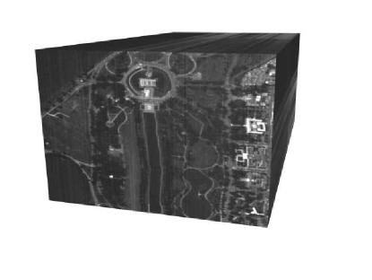
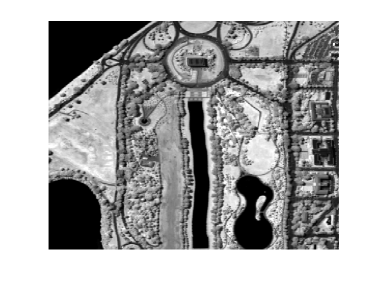
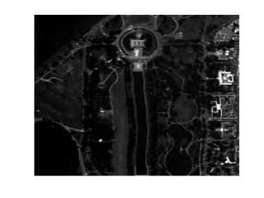
The overflow of data is a critical contemporary challenge in many areas such as information retrieval, biotechnology, textual search, hyper-spectral sensing, classification etc. It is commonly manifested by a high dimensional representation of data observations. A dimension of a data observation is the number of values that describes it. A simple example is an ordinary color image where each pixel has 3 values that represent the red, green and blue values. In this example, the dimensionality is low (equals to 3), however in hyper-spectral images, the dimensionality can reach several hundreds (each value corresponds to a different wavelength of the spectrum). Figure 1.1 illustrates a hyper-spectral image, which is also referred as a hyper-spectral cube (see Chapter 5). The image is a birds-eye view of Washington DC mall, USA, and its surroundings. The images that correspond to two of the wavelengths are given in Fig. 1.2. Images such as those in Figs. 1.1 and 1.2 are common in remote sensing applications e.g. segmentation and anomalies detection (see Chapter 6).
 |
 |
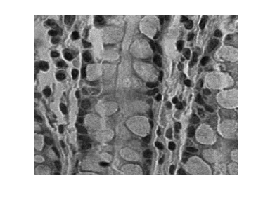
Hyper-spectral images are also used in medical applications such as detection of tissue anomalies. In this case a hyper-spectral microscope is used to capture hyper-spectral images of tissue samples. These images are analyzed in order to detect benign and malignant tumors [144, 145, 56]. Figure 1.3 shows two wavelengths of a hyper-spectral microscope-generated image of a human colon tissue. A more comprehensive introduction on hyper-spectral imagery, can be found in Chapter 5.
 |
Another area that uses high-dimensional data is information retrieval. Applications in this area include text mining, search engines (Google™search is one typical example), etc. In order to process text documents, they must be represented as a vector [133]. One possible high-dimensional representation of a text document is a vector whose coordinates contain the number of occurrences of common and uncommon words.
Financial data such as credit transactions, loan payments and transactions in banking monitoring systems are also examples for high-dimensional data. Data-mining applications such as fraud detection and credit-rate evaluation commonly use high-dimensional financial data to infer behavior characteristics of clients. One representation of high-dimensional financial-data is transaction amounts along time periods whose length is predefined.
The main problem of high dimensional data is the so called curse of dimensionality, which means that in a large number of algorithms the complexity grows exponentially with the increase of the dimensionality of the input data [110]. Furthermore, in certain situations, the number of observations is not sufficient to produce satisfactory reduction of dimensionality [16].
Commonly, the acquiring sensor produces data whose dimensionality is much higher than the actual degrees of freedom of the data. Unfortunately, this phenomenon is usually unavoidable due to the inability (lack of knowledge which values from the sensor are more important for the task at hand) to produce a special sensor for each application. Consider for example a task that separates red objects from green objects using an off-the-shelf digital camera. In this case, a the camera will produce, in addition to the red and green channels, a blue channel, which is unnecessary for this task.
In order to efficiently process high-dimensional datasets, one must first analyze their geometrical structure and detect the actual degrees of freedom, which are manifested by a (small) number of parameters that govern the structure of the dataset. This number is referred to as the intrinsic dimension (ID) of the dataset. Consequently, the information that is conveyed by the dataset can be described by a set of vectors whose dimension is equal to the ID of the original dataset.
There is a direct connection between the intrinsic dimensionality of the data and the degrees of freedom of the observations. This is one of the key motivations for trying to reduce the dimensionality of the observed data. Commonly, correlation exists between some subsets of the observation variables. Hence, it is reasonable to try and find a mapping that embeds the data into a low-dimensional space in which the data is represented by a small number of uncorrelated variables. This embedding can additionally reveal hidden information in the original data, even before subsequent algorithms are applied. The loss of information, which is due to the dimensionality reduction, is not always a disadvantage, on the contrary, the lost information is in many cases not essential, for example information which is due to noise.
The process of finding a low-dimensional representation is called dimensionality reduction. Dimensionality reduction is also referred to as manifold learning. An ID that is lower than the dimension of the ambient space, means that the dataset lies near or on a manifold whose dimension is equal to the ID. Local dimensionality reduction techniques, which are introduced in Section 2.2, are better defined as manifold learning techniques since they investigate local neighborhoods, which usually have a simple structure, in order to reveal the global and usually more complicated structure of the dataset.
One of the most important applications of dimensionality reduction is visualization of high-dimensional datasets. This is facilitated when the dimension of the reduced space is not greater than three. The high-dimensional set is visualized by a plot of its low-dimensional embedding. Since most dimensionality techniques are designed to produce a low-dimensional embedding that preserves the geometry of the original high-dimensional set, the visualized results provide valuable information regarding the geometry of the dataset at hand.
Contribution of this thesis
The contribution of this thesis is two-fold. First, a novel method for dimensionality reduction - Diffusion Bases - is introduced. The method is based on the diffusion map dimensionality reduction algorithm and the theoretical connection between the methods is described. The applicative effectiveness of the diffusion bases method is demonstrated for the segmentation of images that originate from various domains - hyper-spectral imagery, multi-contrast MRI and video.
Second, this thesis shows that dimensionality reduction is an effective tool for solving problems from various domains, namely, identification of materials via their spectral signatures, detection of vehicles using their acoustic signatures and detection of vascular diseases using acoustic recordings of blood vessels.
Structure of this thesis
This thesis is composed of three parts. In the first part, we introduce the novel Diffusion Bases methodology (theory, algorithms and applications) for dimensionality reduction. Specifically, in Chapter 2 we give an in depth introduction to dimensionality reduction where we provide a formal definition of the problem followed by a description of the current state-of-the-art techniques for dimensionality reduction. In Chapter 3 we describe in details the diffusion maps technique [45] since it is closely connected to our diffusion Bases (DB) dimensionality reduction scheme which we introduce in Chapter 4. The DB algorithm explores the variability among the coordinates of the original data while the DM explores local neighborhoods of points in the dataset. Both algorithms use a random walk model. The DB algorithm uses the eigenvectors of the corresponding Markov matrix as an orthonormal system and projects the original data onto it to obtain the low-dimensional representation. The DM algorithm, on the other hand, builds a different Markov matrix whose eigenvectors constitute the low-dimensional representation. In Chapter 5 we provide an introduction to hyper-spectral imagery which includes the terminology, concept, motivation and common applications in this area. Chapter 5 is necessary for the understanding of Chapters 6 and 9. Chapters 6-8 include successful applications of the DB scheme. Specifically, in Chapter 6, the DB dimensionality reduction scheme is used for segmentation of hyper-spectral images and for the detection of anomalies in images of this type. In Chapter 7, the DB scheme is incorporated in an algorithm for segmentation of multi-contrast MRI images. Segmentation of video sequences which uses the DB scheme is described in Chapter 8.
In the second part of this thesis, we present two methods for uniquely identifying materials according to their spectral signatures. Given a spectral signature of a material to be identified, the first method seeks an exact match in a database of spectral signatures while the second method takes into account noise and looks for an approximate identification. Both methods reduce the dimensionality of the spectral signatures by means of feature extraction.
In the third part, we introduce two methods for the detection and classification of predefined events in acoustic signals. The first method is tailored for the detection of vehicles in acoustic signals that were recorded in various terrains where noise and background sounds are present. The second method detects hyper-tension and cardio-vascular diseases according to recordings of vascular vessels. Both methods reduce the dimensionality of the recordings in order to extract features which uniquely characterize the various events that need to be detected and classified.
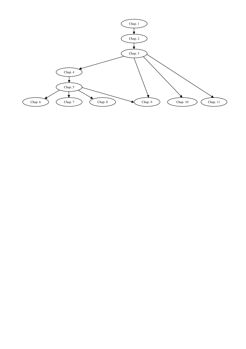
This thesis is based on the following papers: [187], [190], [188], [7], [8], [13] and [189]. Table 1.1 associates the chapters with the papers. Figure 1.4 illustrates the connections and dependencies between the chapters. It indicates the order in which the chapters are to be read. For example, in order to read Chapters 6-8, Chapters 1-5 have to be read first.
| Paper | Chapter |
|---|---|
| [187] | 4, 6 |
| [190] | 7 |
| [188] | 8 |
| [7], [8] | 9 |
| [13] | 10 |
| [189] | 11 |
Chapter 2 Dimensionality Reduction
In this chapter, we describe in detail the current state-of-the-art techniques for dimensionality reduction. We focus on a set of methods that we feel span most of the different approaches to tackle the dimensionality reduction problem while providing references to other available methods.
Notation
The following notation are used throughout this chapter. We denote a original high-dimensional dataset as a set of column vectors
| (2.1) |
where , is the (high) dimension and is the size of the dataset. All dimensionality reduction methods embed the vectors into a lower dimensional space where . Their output is a set of column vectors in the lower dimensional space
| (2.2) |
where approximates the ID (Chapter 1) of . We refer to the vectors in the set as the embedding vectors.
Previous work
The general problem of dimensionality reduction has been extensively researched. In their pioneering work, Johnson and Lindenstrauss [111] laid the theoretical foundations by proving the feasibility of dimension reduction. Specifically, they showed that points in dimensional space can almost always be projected onto a space of dimension with control on the ratio of distances and the error (distortion). Bourgain [23] showed that any metric space with points can be embedded by a bi-Lipschitz map into an Euclidean space of dimension with a bi-Lipschitz constant of . Various randomized versions of this theorem are used for protein mapping [139] and for reconstruction of frequency sparse signals [30, 67].
We classify current dimensionality reduction methods into two categories: global and local methods. Although all methods seek to maintain global properties of the dataset, they differ in the way they accomplish this. Global methods (Section 2.1) first extract the properties they aim to maintain from the high-dimensional dataset and then seek to embed the data into a low-dimensional space while preserving the extracted properties for all the high-dimensional points. Local methods (Section 2.2), on the other hand, utilize the Newtonian paradigm according to which a global description of a system can be derived by the aggregation of local transitions.
2.1 Global methods
In the following, we describe common available global methods for dimensionality reduction.
2.1.1 Principal Component Analysis (PCA)
PCA [103] finds a low-dimensional embedding of the data points that best preserves their variance as measured in the high-dimensional input space. As a preliminary step, the vectors in are centered around the origin. Let be the set centered at the origin where . We define a matrix whose columns are comprised of the vectors
The covariance matrix of the set is computed by is a symmetric matrix that captures the correlations between all possible pairs of measurements. An eigen-decomposition of is performed to produce a set of eigenvalues and their corresponding eigenvectors . The eigenvector gives the direction where the variance of the data is maximal. The magnitude of this variance is given by . In a similar way, the eigenvector gives the direction of the second largest variance , and so on.
The low dimensional vector , which is the embedding of , is given by the projection of onto the first eigenvectors :
where denotes the inner product operator.
One can find many applications spanning a wide range of domains that successfully apply PCA. These include seismology [170], face recognition [216], coin classification [105] to name a few.
The size of the covariance matrix depends on the dimensionality of the vectors in . Consequently, the computation of the covariance matrix may be impossible when the dimensionality of is very high. In such cases, one can use approximation techniques [166]. Furthermore, PCA is only able to discover the true structure of data in case it lies on or near a linear subspace of the high-dimensional input space [150]. This pitfall is crucial since many datasets contain nonlinear structures.
2.1.2 Kernel PCA (KPCA)
KPCA [191] is a generalization of PCA that is able to detect non-linear structures. This ability relies on the kernel trick: any algorithm whose description involves only dot products and does not require explicit usage of the variables can be extended to a non-linear version by using Mercer kernels [192]. When this principle is applied to dimensionality reduction it means that non-linear structures correspond to linear structures in high-dimensional spaces.
In order to linearize a structure, one must find a transformation into a high-dimensional space which maps the original non-linear structure to a high-dimensional linear structure. Finding this is not a trivial task. Fortunately, this can be accomplished by applying a non-linear kernel on the pair-wise inner products.
In KPCA, the covariance matrix is substituted by a pair-wise kernel matrix
According to the kernel trick we have where is the linearizing transformation to a high-dimensional space and denotes the inner product operator.
Centering of the points in the high-dimensional space is achieved by
| (2.3) |
An eigen-decomposition of is performed to produce a set of eigenvalues and their corresponding eigenvectors . The embedding of into is given by:
where is the -th column of the matrix .
Choosing the kernel that achieves the best dimensionality reduction for a given dataset is an open problem and is highly dependent on the dataset at hand (this property is shared with the diffusion map algorithm which is described in Chapter 3). Common choices for kernels are linear kernel in which case KPCA coincides with PCA, Gaussian kernels [192, 196], Polynomial kernels [192, 196] and hyperbolic tangent [192] which is common in neural networks.
2.1.3 Multidimensional Scaling (MDS)
MDS [129, 52] algorithms find an embedding that best preserves the inter-point distances among the vectors in . The input to the algorithms is a matrix that contains all pair-wise distances or dissimilarities. The output is a set of points in a low-dimensional space - usually, the Euclidean space.
The embedding is facilitated by minimizing a loss/cost function which is also known as a stress function. This function measures the error between the pairwise distances among the vectors in and . A common cost function is the raw stress function which is given by
where is the used distance measure.
Another choice for a cost function is the Sammons cost function which is defined as
The minimization of the stress function is obtained by applying common optimization methods such as the conjugate gradient method, the pseudo-Newton technique [52] or by performing spectral decomposition of the pairwise dissimilarity matrix. Metric multidimensional scaling algorithms generalize the optimization procedure to a variety of stress functions and weighted input matrices - however, the result is still given in Euclidean space.
MDS enables the visualization of high-dimensional datasets when the embedding space is or . This property was used for numerous applications such as fMRI data analysis [207] and molecular modeling [219] to name a few. Variations of the MDS algorithm have been proposed. These include Stochastic Proximity Embedding (SPE) [4], FastMap [75] and Stochastic Neighbor Embedding (SNE) [96]. In fact, the ISOMAP algorithm, which is described below, may be considered as a special case of metric multidimensional scaling where the geodesic distance measure constitutes the metric.
2.1.3.1 Generalized multidimensional scaling (GMDS)
Generalized multidimensional scaling [27] generalizes the classical Metric multidimensional scaling by allowing any valid metric space to be used for the output. One of the important uses facilitated by this extension is the representation of the intrinsic metric structure of one surface in terms of the intrinsic geometry of another (also known as the isometric representation problem). Furthermore, using a distance measure111It is not exactly a distance measure since it does not possess all the required properties of a distance measure. that is derived from the Gromov-Hausdorff distance [86], one can compute the partial embedding distance between two surfaces, thus facilitating the partial matching of surfaces. GMDS also allows to find local differences between two shapes.
Formally, let and be given two datasets representing the sampled surfaces of two continuous surfaces and , respectively. The geodesic distances between the samples and are given by the and matrices and , respectively.
The general stress function is defined as
for and
for where the matrix represents the positions of points on in some local or global parametric coordinates , and is a symmetric matrix of nonnegative weights. It should be noted that (a) the metric in the embedding space is not given analytically and is approximated numerically and (b) the norm of the classical MDS algorithm is generalized to the norm.
2.1.4 Summary
Classical techniques for dimensionality reduction such as PCA and MDS, are simple to implement and can be efficiently computed. However, the pitfall of these methods is that they are global i.e. they take into account the distances between all pairs of points. This makes them highly sensitive to noise and outliers since the embedding requires to take into account all the outlier and noise. By taking into account the outliers, the embedding may deviate from the normal data. This pitfall is amended by local methods for dimensionality reduction which are described next.
Beyer et al. [20] show that under a wide variety of conditions, inspection of nearest neighbors is not meaningful. Specifically, they show that as the dimension increases the difference between the distance to the nearest neighbor and the farthest neighbor diminishes and thus renders the nearest neighbor notion practically meaningless. Consequently, using distance as a similarity measurement must be used with caution. This phenomenon may occur even at 10 to 15 dimensions.
2.2 Local methods
Local-information-preserving dimensionality reduction methods (which we refer to as local methods in short) are based on the assumption that the only relevant information lies in local distance measurements. These measurements vary and are usually a function of the Euclidean distance (see below). Accordingly, they look for a low-dimensional embeddings that preserve only local properties of the high-dimensional set. Utilizing the Newtonian paradigm, these methods derive the global geometry of the dataset by aggregating the local information i.e. consider for each point only the information which is inherent in its closest neighboring points. By doing so, they can identify and thus give less importance to outliers and thereby produce an embedding that better fits the original dataset. In this sense, local methods amend the pitfall of global methods.
An interesting property of local dimensionality methods is that they can be formulated using the KPCA framework. This is facilitated by tailoring an appropriate kernel function to each of the methods.
2.2.1 Laplacian Eigenmaps
Laplacian Eigenmaps [15] aim at embedding low dimensional manifolds that reside in a high-dimensional ambient space. It finds a low-dimensional embedding that best preserves the distance from each point only to its closest neighbors. This is in contrast to MDS where the embedding attempt to minimize all pair-wise distances.
The algorithm consists of three steps. First, a graph is constructed on where each graph vertex corresponds to a data point. Edges connect each point (vertex) only to its closest neighbors. The closest neighbors of a point can be chosen either as its nearest neighbors or they can be chosen as the points in the -dimensional hyper-ball of radius centered at . Depending on the neighborhood type that is chosen, either or is given as a parameter to the algorithm.
Second, a weight function is chosen for the edges of the graph. This function can be the Gaussian kernel, which is also referred to as the heat kernel ( is given as a parameter):
Alternatively, in order to avoid the parameter , the weight function can be a simple adjacency function, i.e.
It was shown in [15] that when is approximately lying on a submanifold, choosing to be the heat kernel corresponds to an approximation of the heat kernel on the submanifold.
The third and last step of the algorithm minimizes the cost function
Note that minimizing ensures that neighboring points and are mapped to close points since the choice of weights penalizes otherwise. The solution to this minimization problem is obtained by solving the following generalized eigenvector problem:
where is the degree matrix of the graph which is defined as and is the graph Laplacian which is given by The eigenvalues of the solution are denoted by and their corresponding eigenvectors are given by . The embedding of a point into is defined as
where denotes the -th coordinate of the -th eigenvector.
2.2.2 ISOMAP
The main drawback of MDS is that it produces an embedding that tries to preserve all pair-wise Euclidean distances as captured in the high-dimensional space. Using the Euclidean distance may lead to an embedding that does not reflect the geometry of the manifold since a small Euclidean distance between a pair of points does not imply they are close over the manifold. An example where this phenomenon occurs is the Swiss roll manifold [210] which is displayed in Fig. 2.1. Consequently, a dimensionality reduction algorithm that preserves the pair-wise distances over the manifold will produce an embedding that conforms better with the geometry of the manifold. This is exactly what ISOMAP [211] does. Specifically, ISOMAP applies MDS using the geodesic distance measure instead of the Euclidean one. The geodesic distance between a pair of points is defined as the length of the shortest path connecting these points that passes only through points on the manifold.

Initially, a sparse graph whose vertices correspond to the data points in is constructed where edges connect each vertex to its nearest neighbors. The pair-wise geodesic distance matrix is then approximated using either the Dijkstra [63] or the Floyd-Warshall [78] algorithms. Since the graph is sparse, the pair-wise geodesic distances that is produced provides only an estimate to the exact geodesic distances. The low-dimensional embedding is obtained by applying MDS to the pair-wise geodesic distances matrix.
Two main shortcomings of ISOMAP are its topological instability and its requirement for the original dataset to be convex. Its performance is degraded in the presence of graph short-circuits (also known as loops) and holes in the manifold [135]. Manifolds that contain holes are dealt with by dividing the manifold into sub-manifolds without holes [135]. Graph loops can be overcome by removal of nearest neighbors that do not conform with a predefined local linearity constraint [184]. Another approach for handling graph loops is to remove data points which have high total flow in the shortest path algorithms [40].
2.2.3 Local Linear Embedding (LLE)
LLE [178] assumes that the manifold is locally linear. Accordingly, it approximates the geometry of a manifold by fitting hyperplanes to local neighborhoods of points i.e. the manifold is expressed as an aggregation of locally linear patches. To achieve this, every point is formulated as a linear combination of its nearest neighbors, where is given as a parameter to the algorithm. The output of this formulation is a weight matrix . On one hand, an embedding that maps the high-dimensional data into a low-dimensional space can be approximated by a linear mapping. On the other hand, the weights in describe intrinsic geometric properties of the data that are invariant to linear transformations. Combining these facts implies that the same weights will hold for the low-dimensional embedding points as well. Thus, the second step of the algorithm finds the low-dimensional embedding of the points which best preserves the weights of the high-dimensional linear combinations. Thus, the LLE algorithm consists of two steps where each step solves an optimization problem.
The first step finds the linear combination weights that minimize the following cost function
where the constraint is imposed for every .
The second step finds the low-dimensional embedding points which minimize the cost function
with respect to the weights that were found in the first step.
The LLE algorithm successfully embeds non-convex manifold as opposed to the ISOMAP algorithm and is also more robust to short-circuits than ISOMAP. However, LLE performance is degraded when it is applied on manifolds that include holes [108, 137]. Nevertheless, LLE has been successfully applied to image colorization [172], sound source localization [69] and to image super-resolution [35].
2.2.4 Hessian LLE (HLLE)
The Hessian LLE or Hessian eigenmaps [68] algorithm extends the class of datasets whose dimensionality can be successfully reduced by ISOMAP. Specifically, the convexity requirement is relaxed. This method is based on the underlying assumption that the manifold is locally isometric to an open, connected subset in the low-dimensional space. In order to reduce the dimensionality of a -functional, which measures the average curviness over the manifold, is introduced. The -functional is derived by aggregating all point-wise local Hessian estimations. The Hessian is required to be invariant to the position of the point and therefore is represented in the local tangent space. The low-dimensional embedding is obtained by minimization of with respect to the Frobenius norm.
The embedding algorithm consists of the following steps: first, the basis of the local tangent space is calculated at each point by applying PCA to its nearest neighbors. Next, a matrix whose columns comprise of a column of ones and all cross products of the basis vectors up to the -th order, is constructed. Gram-Schmidt orthogonalization is applied to and the representation of the local Hessian in the tangent space is estimated using the last columns of . Then, the -functional is constructed as where is the Frobenius norm. This functional is minimized via its eigen-decomposition in order to approximate its null space. The -dimensional subspace corresponding to the smallest eigenvalues are extracted. There will be a zero eigenvalue that is associated with the subspace of constant functions. The next eigenvalues correspond to eigenvectors spanning a -dimensional space where our embedding coordinates are to be found. Finally, a basis for is selected. This basis must constitute an orthonormal basis when it is restricted to a specific fixed neighborhood (which may be chosen arbitrarily from those used in the algorithm). The embedding of a point into is obtained as
2.2.5 Local Tangent Space Analysis (LTSA)
LTSA [237] shares with HLLE the property of using the local tangent space in order to discover and represent local properties of . It assumes local linearity of the manifold. This assumption implies that a high-dimensional point and its corresponding low-dimensional point can be mapped to the same local tangent space via two linear transformations. LTSA looks for both a low-dimensional embedding and a linear transformation the maps the low dimensional embedding into the local tangent space of .
Initially, in a similar manner to HLLE, the basis of the local tangent space is calculated at each point by applying PCA to its nearest neighbors. We denote by the low-dimensional embedding of the points in the neighborhood of . Using the property from the last paragraph, an embedding and a linear transformation that minimize are calculated where is the centering matrix of size and is the Frobenius norm.
2.2.6 Random projections
Random projection [67] is a technique whose theoretical foundation stems from the works of Johnson and Lindenstrauss [111] and Bourgain [23] as referenced in the beginning of Section 2. In order to reduce the dimensionality of using random projections, a random basis is first generated where . Two common choices for generating a random basis are:
-
1.
The vectors are uniformly distributed over the dimensional unit sphere.
-
2.
The elements of the vectors are chosen from a Bernoulli +1/-1 distribution and the vectors are normalized so that for .
Next, a matrix whose columns are composed of the vectors in , is constructed. The embedding of is obtained by
2.2.7 Multilayer autoencoders
Multilayer autoencoders [59, 97] use feed-forward neural networks which have an odd number of hidden layers. These networks are tailored for dimensionality reduction by setting the input and output layers to have nodes ( recall that is the dimension of the original dataset while setting the middle layer to contain nodes ( is the dimension of the embedding space). Accordingly, must be given as input to the algorithm. The data points in are input to the network and the network is trained so that the mean square error between the input and the output is minimized. The embedding of a data point is determined according to the values of the nodes in the middle layer when it is fed to the network. Using linear neurons produces similar results to PCA [130] and classical MDS [52] while non-linear dimensionality reduction is obtained by using non-linear activation functions such as Sigmoids.
Backpropagation is usually a poor approach for training multilayer autoencoders since it converges slowly and is sensitive to local minima due to the high number of connections in the autoencoder. In order to overcome this difficulty, several approaches were proposed. Restricted Boltzmann Machines [95] were used in [97] for pre-training using simulated annealing [118]. Following the pre-training, backpropagation was applied to the network in order to fine-tune its weights. Genetic algorithms can also be used for training multilayer autoencoders [99, 174].
2.2.8 Self-Organizing Maps
Self-Organizing Maps [120, 85, 100] are a neural network algorithm which embeds the high dimensional data into a 2D or 3D space. The low-dimensional embedding is called a map and one of the primary uses of this method is visualization of high-dimensional data. The algorithm uses a deformable template to translate data similarities into spatial relationships. The template consists of nodes in a grid formation (hexagonal or rectangular) which discretisize the low-dimensional space. Each node is associated with a position in the map space and a weight vector of the same dimension as the input data vectors.
The training consists of an iterative procedure that performs the following. For each training vector , find the node whose weight is the closest to according to the Euclidean distance. Update its weights and its map neighbors so they become closer to :
where is a monotonically decreasing learning coefficient and is a neighborhood function that depends on the grid distances between and closest node to .
Embedding of a vector to the map is done by assigning the map coordinates of the node whose weight vector is the closest to .
2.2.9 Generative Topographic Mapping
Generative topographic map (GTM) [21, 221, 163] is a probabilistic method that, similarly to SOM, embeds high-dimensional data in 2D or 3D space using a discrete grid to describe the latent space. The algorithm assumes that the high-dimensional data was generated by a smooth non-linear mapping of low-dimensional data into the high-dimensional space and addition of Gaussian noise to it. The Gaussian noise assumption renders the model a constrained mixture of Gaussians. The nonlinear mapping using a radial basis function network (RBF). Given the training data, the parameters of the mapping, the noise and the low-dimensional probability distribution are learned using the expectation-maximization (EM) algorithm.
2.2.10 Other methods
One can find additional methods for dimensionality reduction which can be regarded as variants of the above methods. These include Kernel Maps [206], Conformal Eigenmaps [195], Principal Curves [36], Geodesic Nullspace Analysis [25], Maximum Variance Unfolding [226], Stochastic Proximity Embedding [4], FastMap [75], Locality Preserving Projection [91] and various methods that perform alignment of local linear models [209, 24, 177, 220].
Chapter 3 The Diffusion Maps (DM) Algorithm
Recently, Coifman and Lafon [45] introduced the Diffusion Maps (DM) scheme which is used for manifold learning. DM embed high dimensional data into a Euclidean space of substantially smaller dimension while preserving the geometry of the dataset. The global geometry is preserved by maintaining the local neighborhood geometry of each point in the dataset - a property that classifies it as a local method (see Section 2.2). However, DM use a random walk distance that is more robust to noise since it takes into account all the paths connecting a pair of points. Furthermore, DM can provide parametrization of the data when only a point-wise similarity matrix is available - a property it shares with MDS. This may occur either when there is no access to the original data or when the original data consists of abstract objects.
Given a set of data points as defined in Section 2.1, the DM algorithm includes the following steps:
-
1.
Construction of an undirected graph on with a weight function that corresponds to the local point-wise similarity between the points in 111 is sparse since only the points in the local neighborhood of each point are considered. Wider neighborhood are explored via a diffusion process. . In case we are only given this step is skipped.
-
2.
Derivation of a random walk on the graph via a Markov transition matrix that is derived from .
-
3.
Eigen-decomposition of .
By designing a local geometry that reflects quantities of interest, it is possible to construct a diffusion operator whose eigen-decomposition enables the embedding of into a space of substantially lower dimension. The Euclidean distance between a pair of points in the reduced space defines a diffusion metric that measures the proximity of points in terms of their connectivity in the original space. Specifically, the Euclidean distance between a pair of points, in , is equal to the random walk distance between the corresponding pair of points in the original space.
The eigenvalues and eigenfunctions of define a natural embedding of the data through the diffusion map. Furthermore, the study of the eigenvalues allows us to use the eigenfunctions for dimensionality reduction.
3.1 Building the graph and the weight function
Let be a set of points in as defined in Eq. 2.1. We construct the graph , on in order to study the intrinsic geometry of this set. A weight function , which measures the pairwise similarity between the points, is introduced. For all , the weight function has the following properties:
-
•
symmetry:
-
•
non-negativity:
-
•
fast decay: given a scale parameter , when and when . The sparsity of is a result of this property.
Note that the parameter defines a notion of neighborhood. In this sense, defines the local geometry of by providing a first-order pairwise similarity measure for -neighborhoods of every point . Higher order similarities are derived through a diffusion process. A common choice for is the Gaussian kernel
| (3.1) |
However, other weight functions can be used and the choice of the weight function essentially depends on the application at hand. An automatic procedure for choosing is described in Section 3.4.
3.2 Construction of the normalized graph Laplacian
The non-negativity property of allows to normalize it into a Markov transition matrix where the states of the corresponding Markov process are the data points. This enables to analyze via a random walk.
Formally, is constructed as follows:
| (3.2) |
where
| (3.3) |
is the degree of . If we let be a diagonal matrix where , and we let be the weight matrix that corresponds to the weight function , can be derived as
| (3.4) |
is a Markov matrix since it is row stochastic i.e. the sum of each row in is 1 and , . Thus, can be viewed as the probability to move from to in a single time step. By raising this quantity to a power , this influence is propagated to nodes in the neighborhood of and and the result is the probability for this move in time steps. We denote this probability by and it can be defined by induction:
These probabilities measure the connectivity of the points within the graph. The parameter controls the scale of the neighborhood in addition to the scale control provided by .
3.3 Eigen-decomposition
The close relation between the asymptotic behavior of , i.e. the properties of its eigen-decomposition and the clusters that are inherent in the data, was explored in [41, 79]. We denote the left and the right bi-orthogonal eigenvectors of by and , respectively. Let be the eigenvalues of where .
It is well known that Coifman et al. [47] show that for a finite time we have
| (3.5) |
An appropriate choice of achieves a fast decay of . Thus, to achieve a relative accuracy , only a few terms are required in the sum in Eq. 3.5. By accuracy, we mean that is chosen such that
| (3.6) |
Due to the fast decay of , we will typically have A simple linear search procedure is used to calculate
Coifman and Lafon [45] introduced the diffusion distance
| (3.7) |
This formulation is derived from the known random walk distance in Potential Theory: where 2 is due to the fact that the graph is undirected.
Averaging along all the paths from to results in a distance measure that is more robust to noise and topological short-circuits than the geodesic distance or the shortest-path distance which are used in the ISOMAP algorithm [211]. Finally, the diffusion distance can be expressed in terms of the right eigenvectors of (see [132] for a proof):
| (3.8) |
The sum starts from 2 since is constant. It follows that in order to compute the diffusion distance, one can simply use the right eigenvectors of . Moreover, this facilitates the embedding of the original points in a Euclidean space by:
| (3.9) |
which also provides coordinates on the set . Essentially, due to the fast decay of the eigenvalues of . Furthermore, depends only on the primary intrinsic variability of the data as captured by the random walk and not on the original dimensionality of the data. This data-driven method enables the parametrization of any set of points - abstract or not - provided the similarity matrix of the points is available.
3.4 Choosing
The choice of is critical to achieve the optimal performance of the DM algorithm (and also for the DB algorithm that will be introduced in Chapter 4) since it defines the size of the local neighborhood of each point. On one hand, a large produces a coarse analysis of the data as the neighborhood of each point will contain a large number of points. In this case, the similarity weight will be close to one for most pairs of points. On the other hand, a small might produce many neighborhoods that contain only one point. In this case, the similarity weight will be zero for most pairs of points. Clearly, an adequate choice of lies between these two extreme cases and should be derived from the data.
In the following, we describe an automatic procedure to determine such an for a Gaussian kernel based weight function when the dataset approximately lies on a low dimensional manifold [187]. That is, although is given in the ambient Euclidean space , it is actually restricted to an intrinsic low dimensional manifold . We denote by the intrinsic dimension of . Let be the normalized graph Laplacian [41] where was defined in Eq. 3.4 and is the identity matrix. The matrices and share the same eigenvectors. Furthermore, Singer [198] proved that if the points in are independently uniformly distributed over then with high probability
| (3.10) |
where is a smooth function and is the continuous Laplace-Beltrami operator of the manifold . The error term is composed of a variance term , which is minimized by a large value of , and a bias term , which is minimized by a small value of .
We utilize the scheme that was proposed in [94] and examine the sum of the weight matrix elements
| (3.11) |
as a function of . Let be the volume of the manifold . The sum in Eq. 3.11 can be approximated by its mean value integral
| (3.12) |
provided the variance term in Eq. 3.10 is sufficiently small.
Moreover, we use the fact that for small values of , the manifold looks locally like its tangent space and thus
| (3.13) |
Combining Eqs. 3.11-3.13, we get
Applying logarithm on both sides yields
Consequently, the slope of as a function of on a log-log scale is . However, this slope is only linear in a limited subrange of since and as illustrated in Fig. 3.1. In this subrange, the error terms in Eq. 3.10 are smaller than they are in the rest of the range. Thus, an adequate is chosen from this linear subrange.
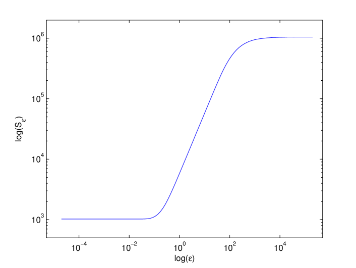
Given the properties of , a simple algorithm for choosing can be devised. First, a graph of on a log-log space is constructed. The axis should range from the of the minimal value to the maximal value of the similarity matrix. If the minimal value is zero, a near zero number should be taken. Given the graph, we look for a section where is (nearly) linear i.e. a linear line. This can be achieved by looking for a near-constant section of the derivative of the graph. We choose from this section.
3.5 Conclusion
In this chapter, the diffusion maps method [45] for dimensionality reduction was introduced. The main contribution of this chapter is a novel algorithm - theory and description - for the automatic derivation of the parameter which is crucial to the performance of the algorithm since it defines the local neighborhood that is examined in the algorithm.
Chapter 4 Diffusion Bases (DB)
Diffusion bases (DB) is a dual algorithm to the DM algorithm in the sense that it explores the variability among the coordinates of the original data [187]. Both algorithms share a graph Laplacian construction, however, the DB algorithm uses the Laplacian eigenvectors as an orthonormal system and projects the original data onto it. The DB algorithm also assumes that there is access to the original data .
Let be the original dataset as defined in Eq. 2.1 and let denote the -th coordinate of , . We define the vector
| (4.1) |
to be the -th coordinate of all the points in . We construct the set The DM algorithm is executed on the set . The right eigenvectors of constitute an orthonormal basis . These eigenvectors capture the non-linear coordinate-wise variability of the original data. This bares some similarity to PCA, however, the diffusion process yields a more accurate estimation of the variability than PCA due to: (a) its ability to capture non-linear manifolds within the data by local exploration of each coordinate; (b) its robustness to noise. Furthermore, this process is more general than PCA and it coincides with it when the weight function (Section 3.1) is linear.
Next, we use the eigenvalue decay property of the eigen-decomposition to extract only the first eigenvectors (we are not excluding the first eigenvector as mentioned in Section 3.3), which contain the non-linear directions with the highest variability of the coordinates of the original dataset .
The dimensionality of is reduced by projecting it onto the basis . Let
| (4.2) |
be the set of these projections, similarly to as it was defined in Eq. 2.2. The embedding of is defined as
and denotes the inner product operator. contains the coordinates of the original points in the orthonormal system whose axes are given by . Alternatively, can be interpreted in the following way: the coordinates of contain the correlation between and the directions given by the vectors in . A summary of the DiffusionBasis procedure is given in Algorithm 4.1.
4.1 Numerical enhancement of the eigen-decomposition
The Markov matrix, which is obtained in Eq. 3.2, is not symmetric. In general, working with a symmetric matrix is faster and more accurate. A symmetric matrix , which is conjugate to , can be obtained in the following way:
| (4.3) |
where and are defined in Eq. 3.3. Let be the eigenvectors of It can be shown (see [41]) that and have the same eigenvalues and that
| (4.4) |
where and are the left and right eigenvectors of , respectively. This leads to modifications of the DM algorithm and the DB algorithm (Algorithm 4.1). The modified DM (abbreviated as MDM from this point on) algorithm calculates the eigenvectors using the symmetric matrix in Eq. 4.3 and applying Eq. 4.4 while the modified DB algorithm (abbreviated as MDB from this point on) projects the data points in onto the orthonormal basis instead of where the number was introduced in Section 3.3. The MDB algorithm is given in Algorithm 4.2.
DiffusionBasis(, , , )
-
1.
Calculate the weight function , (Eq. 3.1).
-
2.
Construct a Markov transition matrix by normalizing the sum of each row in to be 1:
where .
-
3.
Perform eigen-decomposition of
where the left and the right eigenvectors of are given by and , respectively, and are the eigenvalues of in descending order of magnitude.
-
4.
Project the original data onto the orthonormal system to produce:
where
and is the inner product.
-
5.
return .
ModifiedDiffusionBasis(, , , )
-
1.
Calculate the weight function
-
2.
Construct the matrix
where .
-
3.
Perform eigen-decomposition of
where are the eigenvectors of , and are the eigenvalues of in descending order of magnitude.
-
4.
Project the original data onto the orthonormal system to produce:
where
and denotes the inner product.
-
5.
return .
4.2 The algebraic connection between the DM and DB algorithms
Let be a set of vectors as defined in Eq. 2.1. We define weight functions
and
to be used by the modified diffusion maps (MDM) and the modified diffusion bases (MDB) algorithms (Section 4.1), respectively. We denote by and the eigenvectors that are the result of the eigen-decomposition in the MDM and MDB algorithms, respectively. and are orthonormal systems in and , respectively. Accordingly, every coordinate vector can be expressed in as
In a similar manner, every vector can be expressed in as
Let be a matrix whose rows are composed of the vectors in . In this setting, the columns of are given by the coordinate vectors (Eq. 4.1). We define the set where and denotes the cross product. It is easy to verify that is an orthonormal system in . We also define as a row vector by horizontally concatenating its rows
Thus, can be expressed in as
An attempt to directly calculate will involve a weight function of size by which is not feasible even for relatively small values of and . However, we see that can indirectly be calculated as the Cartesian product of the orthonormal bases that result from the eigen-decomposition step in the DM and DB algorithms.
4.3 A graph theoretic link between DB and DM
In this section, we describe a graph theoretic framework that links between the DM and DB algorithms by constructing a special graph. This construction demonstrates the duality between these methods.
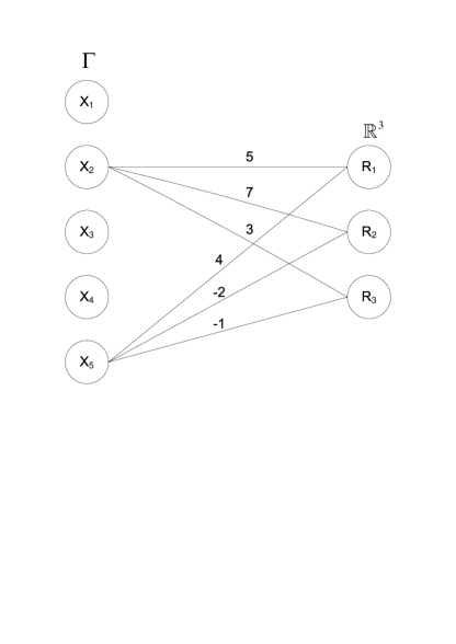
Let be a set of vectors as defined Eq. 2.1. This set of vectors can be represented by a full weighted bi-partite graph where corresponds to the vectors and corresponds to the dimensions of . The weight of each edge is given by - the value in the -th coordinate of the vector which is equal to the -th coordinate of the vector . The size of the weight matrix is . We demonstrate this construction in Fig. 4.1 for the set where the edge weights are specified for and .
For the case of a hyper-spectral cube , the graph construction is as follows. Let be the intensity of wavelength at spatial position where and . We construct a bi-partite graph where correspond to the spatial positions and corresponds to the wavelengths. Their sizes are given by and . A vertex corresponds to the spatial position where denotes the floor operator. The weight of an edge is equal to the -th wavelength intensity at spatial position .
In the following, we describe a construction that corresponds to the kernel that is used in Section 3.1. First, we construct a function which takes a matrix and produces a matrix that depends on and . An example for is the row pairwise correlation where and
| (4.5) |
Another example is the row pairwise squared distances
| (4.6) |
An alternative definition for is a function . In this context, the function (Eq. 4.5) can be defined using when is the inner product. Similarly, (Eq. 4.6) can be defined by when is the squared distance.
Next, we define an element-wise function on a matrix where denotes the result of applying on every element of . We denote by the result of the application of to the element at row and column . With the above definitions, we can define any kernel on for both the DM and the DB algorithms. A DM kernel is constructed from by , while a DB kernel is constructed from by . For example, the Gaussian kernel in Eq. 3.1 can be defined using and .
Given a kernel for which is and is the identity function, DM and DB are connected through the eigenvectors of and . In order to verify this, we look at the singular value decomposition of (assuming there is one). Since and , the result of the eigen-decomposition in the DM and DB algorithms are given by and , respectively.
4.4 Conclusion
In this chapter, a novel method for dimensionality reduction was introduced - diffusion bases. The method is closely related to the diffusion maps algorithm [45]. The algebraic and graph-theoretic connection between the methods was presented. Both methods preserve the geometrical structure of the dataset whose dimension is being reduced.
Table 4.1 summarizes the differences between the DM and DB algorithms. When the number of items in the dataset is higher than the dimensionality of the items (this is the common case), the diffusion bases algorithm has a lower time and space complexity than the diffusion maps algorithm.
| Criterion | DM | DB |
| Similarity matrix is built on | data items | coordinates of the data items |
| Size of similarity matrix | ||
| Time complexity of | ||
| similarity matrix construction | ||
| Embedding mapping |
Chapter 5 Introduction to Hyper-spectral Imagery
A significant recent breakthrough in imagery has been the development of hyper-spectral sensors and software to analyze the resulting image data. Fifteen years ago only spectral remote sensing experts had access to hyper-spectral images or software tools to take advantage of such images. Over the past decade hyper-spectral image analysis has matured into one of the most powerful and fastest growing technologies in fields such as remote sensing and biology to name a few. It is now gradually entering to the area of medical diagnostics.
The “hyper” in hyper-spectral means “over” as in “too many” and refers to the large number of measured wavelength bands. Hyper-spectral images are spectrally overdetermined, which means that they provide ample spectral information to identify and distinguish spectrally unique materials. Hyper-spectral imagery provides the potential for more accurate and detailed information extraction than it is possible with any other type of remotely sensed data. A hyper-spectral cube is a good example for a high dimensional dataset. Therefore, the methods in previous chapters will be applied to these datasets in order to reduce their dimensionality.
In this chapter we review definitions of some basic hyper-spectral concepts and present some recent hyper-spectral image analysis research.
5.1 Spectral imaging: basics
To understand the advantages of hyper-spectral imagery, it may help to first review some basic spectral remote sensing concepts. We recall that each photon of light has a wavelength determined by its energy level. Light and other forms of electromagnetic radiation are commonly described in terms of their wavelengths. For example, visible light has wavelengths between 0.4 and 0.7 microns, while radio waves have wavelengths greater than 30 cm. Reflectance is the percentage of the light hitting a material that is then reflected by that material (as opposed to being absorbed or transmitted). A reflectance spectrum shows the reflectance of a material measured across a range of wavelengths. Some materials will reflect certain wavelengths of light, while other materials will absorb the same wavelengths. These patterns of reflectance and absorption across wavelengths can be used to uniquely identify certain materials. We refer to a unique reflectance pattern of a material as a spectral signature. In Chapter 9 we extract features from spectral signatures in order to uniquely identify materials. These signatures are obtained in laboratory conditions in the wavelength range of nanometer. It should be mentioned that given a sufficient amount of noise and a low spectral resolution (a small number of wavelengths) two signatures might be similar. Nevertheless, this is not the case in the data that is used in this thesis. Our data has high spectral resolution - which is referred to as hyper-spectral (see the next section). This guarantees the uniqueness of the signatures even in the presence of noise.
Field and laboratory spectrometers usually measure reflectance at many narrow, closely spaced spectral bands, so that the resulting spectra appear to be continuous curves. When a spectrometer is used in an imaging sensor, the resulting images record a reflectance spectrum for each pixel in the image. A tutorial on this topic can be found in [153].
5.2 Hyper-spectral data
Most multi-spectral imaging devices measure radiation reflected from a surface at a few wide, separated spectral bands. Most hyper-spectral imagers, on the other hand, measure reflected radiation at a series of narrow and contiguous spectral bands. When we look at a spectrum for one pixel in a hyper-spectral image, it resembles a spectrum that would be measured in a spectroscopy laboratory. This type of detailed pixel spectrum can provide much more information about the surface than a multi-spectral pixel spectrum where multi indicates a lower resolution of captured spectral bands.
Although most hyper-spectral sensors measure hundreds of wavelengths, it is not the number of measured wavelengths that defines a sensor as hyper-spectral but rather it is the narrowness and contiguous nature of the measurements. For example, a sensor that measures only 20 bands could be considered hyper-spectral if those bands were contiguous and, say, 10 nanometer (nm) wide. If a sensor measured 20 spectral bands that were, say, 100 nm wide, or that were separated by non-measured wavelength ranges, the sensor would no longer be considered hyper-spectral.
Standard multi-spectral image classification techniques were generally developed to classify multi-spectral images into broad categories. Hyper-spectral imagery provides an opportunity for more detailed image analysis. For example, using hyper-spectral data, spectrally similar materials can be distinguished, and sub-pixel scale information can be extracted. To materialize this potential, new image processing techniques have been developed. In Chapter 6 we introduce algorithms for segmentation of hyper-spectral images and detection of anomalies (manifested as sub-pixel segments).
5.3 Applications of hyper-spectral image analysis
Hyper-spectral imagery has been used to detect and map a wide variety of materials using their characteristic reflectance spectra. For example, hyper-spectral images have been used by geologists for mineral mapping ([182, 43]) and for detection of soil properties including moisture, organic content, and salinity ([109]). Vegetation scientists have successfully used hyper-spectral imagery to identify vegetation species ([222]), study plant canopy chemistry ([18]), and detect vegetation stress ([2]). Military personnel have used hyper-spectral imagery to detect military vehicles under partial vegetation canopy, and also for many other military target detection objectives.
5.3.1 Medical applications
With new advances in sensor technology and the recent affordability of high-performance spectral imagers, hyper-spectral instruments have enabled a host of new applications - with key efforts in the area of medical imaging. Rather than flying over battlefields, these hyper-spectral sensors can be deployed to scan a patient’s body in search of pre-cancerous regions or to provide much needed spectral information through endoscopy procedures. These hyper-spectral medical instruments hold great potential for non-invasive diagnosis of cancer, assessment of wound conditions, etc. For the patient, tremendous advantage is obtained by being able to not only diagnose the condition in a non-invasive manner but also to potentially treat the condition at the time of diagnosis. Great interest has been generated on behalf of health care providers to investigate the promise of reducing health care costs and timeliness of treatment for many types of disease conditions through the use of hyper-spectral scanning procedures.
Physicians have successfully used hyper-spectral imagery to detect skin tumors. Skin cancers may not be visually obvious since the visual signature may appear as a shape distortion rather than discoloration. Hyper-spectral imaging offers an instant, non-invasive diagnostic procedure (comparing to skin biopsy) based on the analysis of the spectral signatures of skin tissue ([122]). Hyper-spectral imaging was found efficient in providing information regarding the spatial tissue oxygen saturation in patients with peripheral vascular disease ([115]). In addition hyper-spectral imaging systems have been shown to be useful in the monitoring of the spatial distribution of skin oxygenation ([53, 171]), general surgery, plastic surgery, hemorrhagic shock, and burns ([115, 149, 202, 3, 29]).
5.4 Spectral libraries
Spectral libraries are collections of reflectance spectra measured from materials of known composition, usually in the field or laboratory. Many investigators construct spectral libraries of materials from their field sites as part of every project, to facilitate analysis of multi-spectral or hyper-spectral imagery from those sites. Several high quality spectral libraries are also publicly available (e.g. ([152, 87, 72, 123, 180, 181])).
5.5 Classification and target identification
There are many unique image analysis algorithms that have been developed to take advantage of the extensive information contained in hyper-spectral imagery. Most of these algorithms also provide accurate, although more limited, analysis of multi-spectral data. Spectral analysis methods usually compare pixel spectra with a reference spectrum (often called a target). Target spectra can be derived from a variety of sources, including spectral libraries, regions of interest within a spectral image, or individual pixels within a spectral image. The most commonly used hyper-spectral/multi-spectral image analysis methods will be described in Section 9.2.
5.6 Hyper-spectral cameras
Hyper-spectral cameras produce hyper-spectral images of a viewed scene and they gain growing popularity in recent years. These cameras can be installed, for example, on a satellite, on a microscope or on other devices. There are many uses for this type of imagery: biologists use hyper-spectral images of human tissues in order to detect malignant cells, while agronomists use remote sensed images of the earth to estimate amounts of crops.
A regular CCD camera provides the geometry of a scene, however, with very limited spectral information as it is equipped with sensors that only capture details that are visible to the naked eye. In contrast, a hyper-spectral image acquisition device is equipped with multiple sensors - each sensor is sensitive to a particular range of the light spectrum. The output of the device contains the reflectance values of a scene at all the wavelengths that the sensors are designed to capture. Thus, a hyper-spectral image is composed of a set of images - one for each wavelength111A hyper-spectral image is sometimes referred to as a hyper-spectral cube of layered images. . We refer to a set of wavelength values at a coordinate as a hyper-pixel. Each hyper-pixel can be represented by a vector in where is the number of wavelengths. This data can be used to achieve inferences that can not be derived from a limited number of wavelengths which are obtained by regular cameras.
An example for a hyper-spectral camera is AVIRIS which stands for Airborne Visible InfraRed Imaging Spectrometer. It captures images in 224 contiguous spectral bands with wavelengths ranging from 400 to 2500 nanometers. Typically, the camera is mounted aboard a NASA ER-2 airplane which flies at approximately 20 km above sea level. In Chapter 9, the spectrum of the signatures is acquired in the range of nanometers. For comparison, a regular camera, on the other hand, captures a scene in the wavelength range of nanometer which is the range visible to the human eye.
Chapter 6 Segmentation and Detection of Anomalies in Hyper-Spectral Images via Diffusion Bases
While intensity images provide only the geometry of a scene, hyper-spectral images offer spectral information as well. This additional information enables the development of novel and efficient techniques for solving classical image processing problems such as segmentation, change detection, etc. A hyper-spectral image can be modeled as a cube of layered images - one layer per wavelength. This cube is processed in order to extract additional information which lies in the spectral domain. Applying classical image processing techniques separately on each layer does not utilize the inter-wavelength spectral properties of the objects in the image. These methods also fail when sub-pixel segmentation is needed, for example in various remote sensing applications.
In this chapter, we present a novel approach for the segmentation of hyper-spectral images. Our approach reduces the dimensionality of the data by embedding it in a low dimensional space while maintaining the coherency of the information that is crucial for the derivation of the segmentation. Furthermore, our algorithm is able to detect anomalies which come in the form of sub-pixel segments.
6.1 Introduction
Every substance in nature has a unique spectral signature (see Section 5.6) which characterizes its physical properties. One can analyze hyper-spectral images using two approaches: (a) understanding the physical nature; (b) Employing image processing and computer vision techniques. Inter-wavelength connections, which are inherent in spectral signatures, can not be utilized when classical image processing techniques are separately applied on each wavelength image. Thus, the entire hyper-spectral cube needs to be processed in order to analyze the physical nature of the scene. Naturally, this has to be done efficiently due to the large volume of the data.
We propose a general framework for automatic segmentation of hyper-spectral volumes by encapsulating both approaches (physical and image processing) via manifold learning. It is based on the diffusion bases scheme (see Chapter 4). Our approach provides a coherent methodology that projects the hyper-spectral cube onto a space of substantially smaller dimension while preserving its geometrical structure. We present a novel segmentation approach that is tailored for the data in the dimension-reduced space. We distinguish between segmentation of areas that contain more than one pixel and sub-pixel segmentation (anomalies detection) that is common in remote sensing. The algorithms for these segmentation types consist of two steps. Both segmentation types share the first step that performs dimensionality reduction. However, the second step is different: sub-pixel segmentation is accomplished by applying a local variance detection scheme while for the other case, we use a histogram-based method to cluster hyper-pixels in the reduced-dimensional space. The proposed algorithm is fast, automatic (no supervision is required) and it is robust to noise, so there is no need for a pre-processing denoising stage.
This chapter is organized as follows: in Section 6.2 we present a survey of related work on segmentation. In Section 6.3 we introduce the two phase Wavelength-wise Global (WWG) hierarchical segmentation algorithm. Section 6.4 contains experimental results from the application of the algorithm on several hyper-spectral volumes. Concluding remarks are given in Section 6.6.
6.2 Related work
We review in this section some current methods for segmentation of still images. For an extensive survey of current state-of-the-art methods for dimensionality reduction the reader is referred to Chapter 2.
Automatic segmentation of still images has been investigated by many researchers from various fields of science. Segmentation methods can be divided into the following groups: Graph-based techniques, boundary-based methods, region-based methods and hybrid methods.
Shi and Malik [197] propose a technique that solves image segmentation as a graph partitioning problem. They define a global criterion, the normalized cut, which is optimized in order to partition the graph. The graph partition induces a binary segmentation of the image. Perona and Freeman [167] propose a fast affinity approximation algorithm,which takes into account only two groups, foreground and background. The foreground group is computed as a factorized approximation of the pairwise affinity of the elements in the scene.
Weiss [227] suggests a unified treatment of three affinity matrix-based algorithms - Shi and Malik [197], Perona and Freeman [167] and Scott and Longuet-Higgins [193]. He shows close connections between them while pointing out their distinguishing features. Their similarities lie in the fact that they all use the eigenvectors of the pairwise similarity matrix. They differ by the eigenvectors they look at and by the ways they normalize the affinity matrix.
Fowlkes et al. [80] propose an approach that is based on a numerical solution of eigenfunction problems, known as the Nyström extension in order to reduce the high computational cost of grouping algorithms that are based on spectral partitioning like the normalized cuts. Belongie et al. [17, 79], present a modification to the previous algorithm that does not require the weighted adjacency matrix to be positive definite.
Boundary-based techniques find objects in the image via their contours. The simplest form of such segmentation is to apply edge-detection [83]. More advanced techniques apply physics-based deformable models that change under the laws of Newton mechanics, in particular, by the theory of elasticity expressed in the Lagrange dynamics. In general, these models start from an initial shape and gradually evolve to the contour of the image objects. One type of these shapes is snakes (also known as active contours), were first introduced by Kass et al. [113]. In a later paper, Zhu et al. [238] propose an algorithm in which the segmentation is derived by minimizing a generalized Bayes/MDL criterion using the variational principle and combining aspects of snakes/balloons and region growing (region-based methods are described below). In a more recent paper [34], Chan and Vese propose a model for active contours to detect objects, based on curve evolution, the Mumford–Shah functional [155] for segmentation and level sets [164]. Their model can detect objects whose boundaries are not necessarily defined by a gradient.
Region-based methods group together similar pixels according to some homogeneity criteria. They assume that pixels, which belong to the same homogeneous region, are more alike than pixels from different homogeneous regions. Examples for these methods are the split-and-merge and the region-growing techniques [37, 101]. In many cases, these methods fail to produce satisfactory segmentation results in the presence of noise.
Another approach to image segmentation uses histograms. However, most of the histogram-based algorithms deal only with gray level images. Dealing with 3D color histograms is a difficult task. The technique in [217] projects 3D color spaces onto 2D or even 1-D spaces and segment the image according to the obtained surfaces. Other techniques [183, 186] transform the 3D histogram into a binary tree where each node corresponds to a different range of RGB values.
Hybrid methods improve the segmentation results by combining the advantages of different techniques. Hybrid techniques gain their advantage by incorporating both global (histogram) and local (regions and boundaries) information. The Watershed algorithm [223] is an example of a hybrid technique. It begins with a boundary based method and continues with a region growing technique. Navon et al. [157] propose an iterative algorithm for segmentation of still color image, which is based on adaptive automatic derivation of local thresholds. The algorithm uses the segmentation result of the watershed algorithm as an initial solution and continues with a region-growing technique.
Some algorithms, which are used for specific image processing tasks such as segmentation, can be extended to handle hyper-spectral data volumes. The normalized cuts algorithm [197] can be extended in a straight forward manner to handle hyper-spectral data. However, this method uses a pixel similarity matrix without attempting to reduce the dimensionality of the data, which renders it to be computational expensive. Furthermore, the choice of pixel similarity metrics can be further investigated to yield better results.
6.3 The wavelength-wise global (WWG) algorithm for
above pixel segmentation
We introduce a two-phase approach for the segmentation of hyper-spectral images. The first stage reduces the dimensionality of the data using the DB algorithm and the second stage applies a histogram-based method to cluster the low-dimensional data.
We model a hyper-spectral image as a three dimensional cube where the first two coordinates correspond to the position and the third coordinate corresponds to the wavelength . Let
| (6.1) |
be a hyper-spectral image cube, where the size of the image is , the number of wavelengths is and is the reflectance value at position at wavelength . An example for a hyper-spectral image cube is illustrated in Fig. 1.1. For notation simplicity, we assume that the images are square. It is important to note that almost always .
can be viewed in two ways:
-
1.
Wavelength-wise: is a collection of images of size where
(6.2) is the image that corresponds to wavelength .
-
2.
Point-wise: is a collection of -dimensional vectors where
(6.3) is the hyper-pixel (see Section 6.1) at position .
The proposed WWG algorithm assumes the wavelength-wise setting of a hyper-spectral image. Note that the DB and DM algorithms receive vectors as their inputs. Thus, we regard each image as a - dimensional vector. Formally, let
| (6.4) |
be a 2D matrix corresponding to where
( is defined in Eq. 6.1). Each column in corresponds to the image at wavelength . We denote by
| (6.5) |
the column vector that corresponds to (see Eq. 6.2).
6.3.1 Phase 1: Reduction of dimensionality via DB
Different sensors can produce values at different scales. Thus, in order to have a uniform scale for all the sensors, each column vector , is normalized to be in the range [0,1]. Then, we form the set of vectors from the columns of and we execute Algorithm 4.1 on . The dimensionality can also be reduced using Algorithm 4.2. In this case, we will refer to the segmentation algorithm as the modified-WWG algorithm. In either case, we denote the low-dimensional embedding by as defined in 4.2.
6.3.2 Phase 2: Segmentation by colors
We introduce a histogram-based segmentation algorithm that extracts objects from using . For notational convenience, we denote by hereinafter. We denote by the cube representation of the set in accordance with Eq. 6.1:
We assume a wavelength-wise setting for Let be a 2D matrix in the setting defined in Eq. 6.4 that corresponds to . Thus, the matrix , corresponds to a column in and , corresponds to a row in . The coordinates of will be referred to as colors from this point on.
The segmentation is achieved by clustering hyper-pixels with similar colors. This is based on the assumption that objects in the image will be composed of hyper-pixels that have similar color vectors in . These colors contain the correlations between the original hyper-pixels and the global inter-wavelength changes of the image. Thus, homogeneous regions in the image have similar correlations with the changes i.e. close colors where closeness between colors is measured by the Euclidean distance.
The segmentation-by-colors algorithm consists of the following steps:
-
1.
Normalization of the input image cube :
First, we normalize each color layer of the image cube to be in [0,1]. Let be the -th ( is the color index) color layer of the image cube . We denote by the normalization of and define it to be(6.6) -
2.
Uniform quantization of the normalized image cube :
Let be the given number of quantization levels. We uniformly quantize every value in to be one of possible values. The quantized matrix is given by :(6.7) where . We denote the quantized color vector at coordinate by
(6.8) -
3.
Construction of the frequency color histogram:
We construct the frequency function where for every , is the number of quantized color vectors , that are equal to . -
4.
Finding peaks in the histogram:
We detect local maximum points (called peaks) of the frequency function . We assume that each peak corresponds to a different object in the image cube . Here we use the classical notion of segmentation - separating object from the background. Indeed, the highest peak corresponds to the largest homogeneous area which is mostly the background. The histogram may have many peaks. Therefore, we apply an iterative procedure in order to find the highest peaks where the number of the sought after peaks is given as a parameter to the algorithm. This parameter corresponds to the number of objects we are looking for. We assume that a peak and its neighborhood in the histogram correspond to a single object in the scene. Accordingly, the next peaks are sought after outside this neighborhood. In order to accomplish this, the algorithm is given an integer parameter , which specifies the size of the neighborhood. This size is defined as the cube with radius around a peak. Formally, we define the -neighborhood of a coordinate to be(6.9) The coordinates outside the neighborhood are the candidates for the locations of new peaks. Thus, the next iterations find the rest of the peaks. The peaks are labeled . The output of this step is a set of vectors
that contains the colors that are associated with the highest peaks. A summary of this step is given in algorithm 6.1.
-
5.
Finding the nearest peak to each color:
Once the highest peaks are found, each quantized color vector is associated with a single peak. The underlying assumption is that the quantized color vectors, which are associated with the same peak, belong to the same object in the color image-cube . Each quantized color is associated with the peak that is the closest to it with respect to the Euclidean distance and it is labeled by the number of its associated peak. We denote bythis mapping function, where
-
6.
Construction of the output image:
The final step assigns a unique color to each coordinate in the image according to its label . We denote the output image of this step by .
PeaksFinder(, , )
-
1.
-
2.
while
-
3.
Find the next global maximum of .
-
4.
Add the coordinates of to .
-
5.
Zero all the values of in the -neighborhood of (Eq. 6.9).
-
6.
end while
-
7.
return .
6.3.3 Hierarchical extension of the WWG algorithm
We construct a hierarchical extension to the WWG algorithm in the following way: given the output of the WWG algorithm, the user can choose one of the objects and apply the WWG algorithm on the original hyper-pixels which belong to this object. Let be the color of the chosen object. We define to be the set of the original hyper-pixels which belong to this object:
This facilitates a drill-down function that enables a finer segmentation of a specific object in the image. We form the set from as described in the beginning of Chapter 4 and run the DiffusionBasis algorithm (Algorithm 4.1 or 4.2) on . Obviously, the size of the input is smaller than that of the original image, thus allowing a finer segmentation of the chosen object. We denote the result of this stage by . Next, the WWG is applied on and the result is given by . The drill-down algorithm is outlined in Algorithm 6.2. This step can be applied on other objects in the image as well as on the drill-down result.
DrillDown(, , , ,)
6.3.4 Sub-pixel segmentation
The first steps of the sub-pixel segmentation procedure are similar to those that are used by the above-pixel segmentation: the dimensionality reduction is used as described in Section 6.3.1 and is normalized according to Eq. 6.6.
Let be the normalized 3D image volume in the dimension-reduced space as described in Eq. 6.6 and let be a hyper-pixel in . Sub-pixel segments have high contrast with hyper-pixels in their local neighborhood. This is manifested by differences in several of their colors (see Section 6.3.2). This is due to the difference in their correlations with the vectors in the diffusion basis. We refer to such color points as isolated points. The following steps are applied in order to detect isolated points.
We define the -neighborhood of to be
We compute the number of pixels in whose differences from are above a given threshold . We denote this number by
If the size of is larger than a given threshold then is classified as an isolated point. determines the number of pixels that are different from in the neighborhood of in order for to be classified as an isolated point.
A coordinate is classified as a sub-pixel segment if there are and such that and are isolated points. The requirement that a coordinate will contain an isolated point in at least two images prevents misclassification of noisy isolated points as sub-pixel segments.
6.4 Experimental results
The results are divided into three parts: (a) segmentation of hyper-spectral microscopy images; (b) segmentation of remote-sensed hyper-spectral images; (c) sub-pixel segmentation of remote-sensed images. We provide the results using the two dimensionality reduction schemes that were described in Algorithms 4.1 and 4.2.
We denote the size of the hyper-spectral images by where the size of every wavelength image is and is the number of wavelengths. The geometry (objects, background, etc.) of each hyper-spectral image is displayed using a gray image . This image is obtained by averaging the hyper-spectral image along the wavelengths. Given a hyper-spectral image of size , is obtained by
We refer to as the wavelength-averaged-version (WAV) of the image. All the results were obtained using the automatic procedure for choosing which is described in Section 3.4.
Segmentation of hyper-spectral microscopy images
Figures 6.1 and 6.2 contain samples of healthy human tissues and the results after applying the WWG algorithm to them. The images are of sizes and , respectively. The images contain three types of substances: cell nuclei, glandular cell cytoplasm and lamina propria cell cytoplasm.
Figure 6.1(a) shows the WAV of the image. Figures 6.1(b) and 6.1(c) show the and wavelengths, respectively. The images in the through the wavelengths are less noisy than the rest. Figures 6.1(d) and 6.1(e) display the results after the application of the WWG and the modified-WWG algorithms, respectively. The algorithm clearly segments this image into three parts: the lamina propria cell cytoplasm is colored in blue, the glandular cell cytoplasm is colored in red and the cell nuclei is colored in green.

|
|
|---|---|
|
|
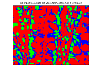
|
Figure 6.2(a) shows the WAV of the image. Figures 6.2(b) and 6.2(c) show the and wavelengths, respectively. The images in the through the wavelengths are less noisy than the rest. Figure 6.2(d) shows results after applying the k-mean algorithm to (a). Figures 6.2(e) and 6.2(f) display the results of the application of the hierarchical extension of the WWG algorithm while Figs. 6.2(g) and 6.2(h) display the results of the application of the hierarchical extension of the modified-WWG algorithm. Figures 6.2(e) and 6.2(g) depict the first iteration of the WWG algorithm and the modified-WWG algorithm, respectively. The second iteration receives as input the hyper-pixels that are in the green region of Figs. 6.2(f) and 6.2(h). The results of the second iteration of the WWG algorithm and the modified-WWG algorithm are shown in Figs. 6.2(f) and 6.2(h), respectively. The image is clearly segmented into three parts. The lamina propria cell cytoplasm is colored in green, the glandular cell cytoplasm is colored in blue and the cell nuclei is colored in red. Both (e) and (g) exhibit better inter-nuclei separation than (d).
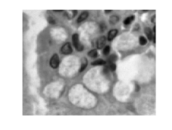
|
|
|---|---|
|
|
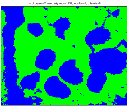
|
|
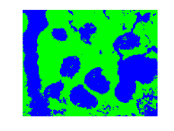
|
Segmentation of remote-sensed images
Figure 6.3 contains a hyper-spectral satellite image of Washington DC mall and the result after applying the WWG algorithm to it. The image is of size . Figure 6.3(a) shows the WAV of the image. The image contains water, two types of grass, trees, two types of roofs, roads, trails and shadow. Figures 6.3(b) and 6.3(c) show the and wavelengths, respectively. Figures 6.3(d) and 6.3(e) are the results of the WWG algorithm and modified-WWG algorithm, respectively, where the water is colored in blue, the grass is colored in two shades of light green, the trees are colored in dark green, the roads are colored in red, the roofs are colored in pink and yellow, the trails are colored in white and the shadow is colored in black.
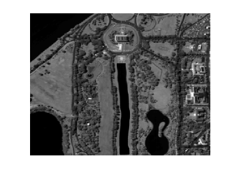
|
|
|---|---|

|
|
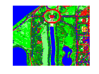
|
Sub-pixel segmentation:
The results of the application of the sub-pixel segmentation algorithm on a hyper-spectral image of a mountain terrain are given in Fig. 6.4. The image was taken from a high altitude airplane and it contains twenty four sub-pixel segments. Figure 6.4(a) shows the WAV of the image. Figures 6.4(b) and 6.4(c) show the and wavelengths, respectively. The noise in the image is caused by atmosphere conditions and calibration errors of the hyper-spectral camera. These problems can be found in most of the wavelengths. Figure 6.4(d) displays with squares around the sub-pixel segments that were found. The dimensionality was reduced using Algorithm 4.2 with . The sub-pixel segmentation was obtained using . The algorithm detects all twenty four segments.
Our algorithm is highly robust to noise as it is demonstrated by the results at the presence of noisy wavelengths which are depicted in Figs. 6.2(b)-6.4(b) and 6.2(c)-6.4(c).
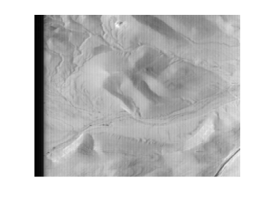
|
|
|---|---|
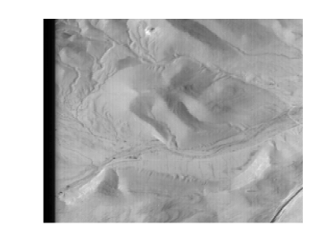
|
6.5 Conclusion
In this chapter, a novel algorithm for the segmentation of hyper-spectral images was introduced. The algorithm utilizes the diffusion bases algorithm which is described in Chapter 4 in order to reduce the dimensionality of the data. Two segmentation algorithms were proposed: one for the segmentation of the dimension-reduced data and the other for the detection of sub-pixel segments i.e. anomalies. The algorithm was successfully applied to images produced by a hyper-spectral microscope and also to remote-sensed images. This demonstrates the broad range of domains the proposed algorithms can tackle.
6.6 Discussion
The results in Section 6.4 were obtained using a Gaussian kernel. It was shown in [45] that any positive semi-definite kernel may be used for the dimensionality reduction. Rigorous analysis of families of kernels to facilitate the derivation of an optimal kernel for a given set is an open problem and is currently being investigated by the authors.
Every hyper-spectral image cube that we tested in Section 6.4 produced a different set of eigenvalues. We assume that the eigenvalues play a vital role in achieving the dimensionality reduction while having unique physical properties. Analysis of the behavior of the eigenvalues is crucial. As a result of this analysis, an automatic algorithm may be constructed for choosing the eigenvectors which will produce the best segmentation results.
The parameter determines the dimensionality of the diffusion space. Automatic choice of this threshold is vital in order to detect the objects in the image cube. A rigorous way for choosing is currently being studied by the authors. Naturally, is data driven (similarly to ) i.e. it depends on the set at hand.
Detection of sub-pixel objects in remote-sensed images is a preliminary step to their identification. These sub-pixel objects are composed of several materials that are mixed. Their identification requires an unmixing algorithm that separates the different substances of the object.
Chapter 7 Neuronal Tissues Sub-Nuclei Segmentation Using Multi-Contrast MRI
Many brain surgeries, forebrain functionality mapping, research of brain-related diseases and additional various pathological procedures rely on a sub-nuclei mapping of the examined neuronal tissue. Using contemporary acquisition tools, to construct a reliable in-vivo sub-nuclei mapping is a highly complex task.
In this chapter we proposes a novel algorithm, called Sub-Nuclei Finder (SNF), which segments neuronal tissues into their sub-nuclei arrangement. Using multi-contrast Magnetic Resonance Imaging (MRI), we are able to separate a neuronal tissue into its sub-nuclei in 3D space. Our approach includes image enhancement, non-linear dimensionality reduction and clustering in 3D space. For the image enhancement, we use a wavelet-based method, which reduces the undesired noise and simultaneously emphasizes and amplifies features of interest. As for the dimensionality reduction procedure, we use the frameworks of Diffusion Maps (Chapter 3) and Diffusion Bases (Chapter 4) to achieve a non-linear local-geometry-driven reduction of dimensionality. In order to segment the enhanced low-dimensional data, we use a Silhouette-Driven K-Means (SDK) algorithm, which automatically identifies the number of clusters for the desired separation.
We demonstrate our algorithm on the Thalamus sub-part of the human brain. Our algorithm successfully segments the human thalamus into its sub-nuclei in strong agreement with a known histological atlas. Moreover, the results on a number of healthy subjects are highly correlated.
7.1 Introduction and related work
We introduce a novel framework for performing a sub-nuclei segmentation of brain tissue. The proposed framework is comprised of a special MRI-based acquisition method and a new algorithm for the segmentation task. In this section, we survey a number of issues that are relevant to this framework. We explore each issue including its significant related work. We start by describing in Sections 7.1.1 and 7.1.2 the problem of sub-nuclei segmentation that motivates this chapter. Then, we explore the issues that are relevant to the proposed Sub-Nuclei Finder (SNF) algorithm, which are: image enhancement in Section 7.1.3 and cluster analysis in Section 7.1.4. Dimensionality reduction is also a key part of the proposed scheme and it was explored in Chapter 2.
The rest of this chapter is organized as follows: in Section 7.2, we describe two of the building blocks of the SNF algorithm. Namely, a wavelet-based image-enhancement technique and a silhouette-driven K-Means clustering technique. These techniques are used by the SNF algorithm which is described in Section 7.3. Experimental results are given in Section 7.4. We conclude in Section 7.5.
7.1.1 The problem of sub-nuclei segmentation
The ability to map a neuronal tissue to its sub-parts, including its sub-nuclei arrangement, is needed for certain brain surgeries, forebrain functionality mapping and for pathologically tracking and researching brain related diseases.
In the field of functional brain studies (e.g. fMRI), changes in the functional-activation have been detected relating certain diseases [22, 93, 173, 179, 224, 225]. An accurate mapping of the brain is necessary for accurately locating the specific areas of these changes.
In order to further comprehend the necessity of a sub-nuclei mapping, we take the thalamus as a case-study. The thalamus is a large ovoid mass of gray matter situated in the posterior part of the forebrain. It functions as a central relay station conveying sensory impulses from the spinal cord to the cerebrum. A number of sub-parts which are known as nuclei constitute the thalamus. Each nuclei has its own function and cyto-architecture (cellular composition). Most of the histological researches [154, 185, 200, 218] have detected 9-16 major nuclei. Figure 7.1 shows a 3D scheme of the major nuclei in the human thalamus.
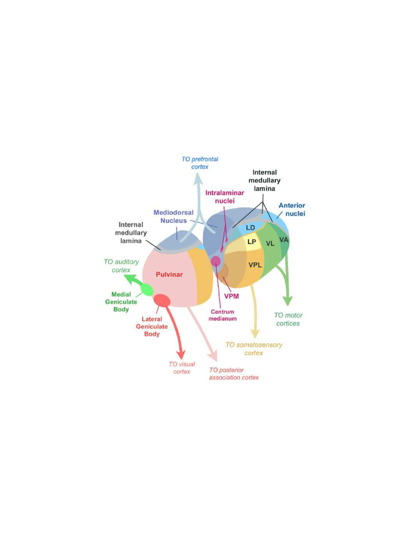
Changes in the thalamus nuclei have been observed in a large number of diseases, e.g. Parkinson’s disease [82], Wallerian degeneration [161], chronic pain syndrome [58], multiple sclerosis [51] and schizophrenia [28]. In some of these diseases the treatment can include a removal by surgery or an electric stimulation of the involved nucleus/nuclei [214].
Moreover, we indicate that using a nuclei map, based on one brain, for another different brain, is problematic due to the wide variability that exists in the nuclei sizes and locations in each brain of each individual [218].
7.1.2 Sub-nuclei segmentation using MRI
Standard usage of existing acquisition methods such as Computer Tomography (CT) and Magnetic Resonance Imaging (MRI) does not provide adequate contrast for distinguishing between nuclei. Recently, the medial-dorsal nucleus (MD) of the thalamus has been detected by a standard usage of MRI [146], but without the ability to detect the rest of the thalamus nuclei. Hence, it seems that a promising breakthrough would be a non-standard usage of an existing acquisition method.
MRI has a potential to be a basic sensing method for this task. It satisfies the non-invasive and in-vivo demands and it outperform other sensors in the aspect of resolution and separability capability. Another major advantage of MRI is its multi-contrast methodology (see details below).
The attempts made thus far using standard MRI [5, 6, 136, 205, 234] have obtained a gross segmentation of the brain into its three main compartments: white matter, gray matter and cerebrospinal fluid (CSF). Some of these attempts did a more accurate separation into a small number of sub-cortical parts. As we mentioned above, only one nucleus (MD) of the thalamus has been successfully detected in the standard procedure. In addition, a MRI high-resolution acquisition was done in-vitro delivering an improved separation between the cortical layers [19, 76, 125, 151], though its long acquisition time is not realistic for in-vivo procedures.
Regarding the thalamus, a recent hypothesis argues that its nuclei are distinguished in their characteristic fiber orientation [159, 229, 230]. Indeed, based on this hypothesis, division of the thalamus into several nuclei was made using Diffusion Tensor Imaging (DTI) [112, 231]. DTI is a novel MRI-based technique, which enables the visualization of the location, orientation and anisotropy of the white matter tracts of the brain.
As aforementioned, one of the major advantages of MRI is that it is a multi-contrast method. Namely, controlling several parameters of the acquisition process (such as time to repeat, time to echo, etc.), one can affect the produced images contrast. The contrast variability, in accordance with the acquisition parameters, is usually distinctive for each type of neuronal tissue. This is the main motivation for the usage of different contrast acquisition-methods for neuronal tissues separation. In [236], five contrast acquisition-methods were used, which enabled a segmentation of a brain into its white matter, gray matter, CSF and few sub-cortical structures. However, they did not deliver a segmentation of the nuclei level. Yovel and Assaf [235] used ten contrast acquisition-methods and managed to segment a human thalamus into seven histologically-distinct areas.
7.1.3 Image enhancement
Generally speaking, the goal of image enhancement is to process an image such that the achieved result is more suitable than the original image for a defined task. Specifically, it can be said that the goal of image enhancement is to supply techniques that can enhance the obscured details of the features, that are most relevant to a specific application, and simultaneously reduce the noise. For instance, in our work we aim to enhance features, that separate between neuronal tissue nuclei, and also to reduce the noise caused during the acquisition and the quantization processes. Due to the ambiguity in the definition of features and noise, the field of image enhancement is objective and it is application-depended. Hence, there is no general standard of image enhancement quality that can serve as a design criterion for these techniques.
Many solutions have been suggested for image enhancement and we will briefly survey several relevant ones. Histogram modification techniques [81, 106] are attractive due to their simplicity and relative low complexity. These techniques are performed by fixing a transformation (usually a non-linear one) that is applied on the image histogram. This transformation is applied to every pixel in the image and it maps each gray level into a new gray level. However, these techniques suffer from the fact that the local relations between the pixels are not used. Therefore, adaptive histogram equalization methods were developed in order to overcome this restriction. Unfortunately, these methods are usually based on a constant-sized window which is not suitable for emphasizing features of various sizes.
Gorden and Rangayyan [84] presented a method, that is based on adaptive neighborhoods. It emphasizes the interesting features, but at the same time amplified the noise causing digitization artifacts. Another adaptive neighborhoods method was presented in [60, 61, 62], however, it combines knowledge regarding the specific feature that needs to be enhanced. This knowledge dependence is not applicable in our case since the data we work with contains different types of features for which this preliminary knowledge is unavailable. A non-linear stretching of a linear combination of the original image and smoothed versions of it was proposed in [208]. This technique is able to emphasize edges while providing a minimal noise amplification.
Unsharp masking methods [83, 175] sharpen the edges by subtracting a smoothed image (e.g. using a Laplacian filter) from the original image. However, these methods are less effective when they are applied to images that contain features of various sizes (such as in our case where the nuclei sizes vary), due to their linearity and their single scale analysis. An attempt to overcome this limitation is presented in [14, 84] where a local contrast and non-linear transformations are used.
A promising category for image enhancement uses wavelet analysis. The wavelet analysis (transform) consists of a decomposition of a signal (2D signal in case of an image) using a family of functions referred to as the wavelet family. See [55, 148] for a fundamental discussion on wavelets. Contrary to the Fourier transform, which reveals only the frequency attributes of an image, the wavelet transform delivers a powerful insight into both spatial and frequency characteristics of the image and also represents the image in various scales of resolution, referred to as multi-resolution analysis. The variation of resolution enables the transform coefficients to locally characterize the irregularities of the signal (image). Hence, wavelet analysis can provide a basis for sophisticated image enhancement tasks (such as in our case) that outperform other existing techniques.
7.1.4 Cluster analysis
The final step of the SNF algorithm, is a clustering procedure. This step divides the processed data, which is received from the previous steps of the SNF algorithm, into groups. Each group represents a nucleus of the examined neuronal tissue. Next, we present a brief survey of cluster analysis.
Cluster analysis, also known as clustering, is a sub-domain of unsupervised learning. In the field of cluster analysis, a set of objects is divided to an unknown number of clusters. Ideally, the number of clusters should be discovered during the procedure. However, some clustering techniques, e.g. K-Means (see below), require the number of sought after clusters as input. The main guideline for the clustering process is that objects of the same class should be “similar” while objects that belong to different classes should be “dissimilar”.
Data representation affects the results of the clustering procedure. In some cases, balancing this phenomenon can be achieved by a careful selection of a distance metric. For instance, in our case, we use the diffusion metric (Section 3.3). Thus, although commonly successful, clustering analysis is an experimental procedure in its nature.
There exists a large number of clustering techniques. Most of them can be classified into two main categories: hierarchical clustering and partitioning clustering.
In hierarchical clustering techniques, the clusters created during the process are repeatedly combined into larger clusters, resulting in a hierarchical structure in a shape of a tree. For further details regarding this category, the reader is referred to [124].
Partitioning clustering techniques divide the set of objects into homogeneous clusters, which afterwords are examined separately. In these techniques, an object dissimilarity metric is chosen. Moreover, the number of the requested clusters and their initialization must be chosen. Hardy [90] introduces a comparison between different methods for choosing the number of clusters.
In this chapter, we use a technique (Section 7.2.2), which is based of the K-Means clustering algorithm, for the clustering phase of the SNF algorithm. In the following, we briefly describe the K-Means [143] technique, which belongs to the partitioning clustering category. In K-Means, the k signifies the number of clusters that is set a-priori, while the means signifies the way that clusters centroids are calculated. For simplicity, we refer to a data object as a “point”. The K-Means technique uses a two-step iterative algorithm, which minimizes the sum of point-to-centroid squared distances, summed over all k clusters. Initially, the points are assigned at random to the k clusters. In the first step, the centroid of every cluster is calculated by taking the mean across all points in the cluster. In the second step, every point is reassigned to the cluster whose centroid is the closest one to it. These two steps are repeated until there is no further change in the assignment of the data points (the stopping criterion). An undesirable situation is when this process converges to a local optimum, i.e. a partition of points in which is not the optimal (global minimum). This problem can be solved by using a different initialization.
Most of the clustering algorithms are not intended to find the optimal separation, but rather find a separation that gives a local optimum according to a certain criterion used by the algorithm. Nevertheless, there are techniques that find the global optimum. Several of them are described in [102].
The robustness of a clustering algorithm is a critical issue. The term “robustness” used here refers to the following question: if some input data points deviate slightly from their current values, will we get the same clustering result? This deviation is referred to as a perturbation of the original data. A good clustering technique should be insensitive to noise and perturbations of the data and capture the “real” structure of the data. In our case, the robustness to noise and the emphasis of the “interesting” features of the data are achieved using an image enhancement phase (Section 7.2.1) prior to the clustering phase. An extensive source for in-depth discussion on robustness and robust statistics can be found in [104].
7.2 Building blocks of the SNF algorithm
In this section, we describe the methods that are used in the SNF algorithm (Section 7.3) for image enhancement and clustering. First, we describe the method we use for image enhancement and we continue with a description of the method we use for clustering. The DB and DM methods that are used for the dimensionality reduction were described in Chapters 3 and 4.
7.2.1 Wavelet-based image enhancement
This section contains a description of the wavelet-based image enhancement technique which is used in the SNF algorithm. This technique, was originally developed for mammography enhancement ([134]) and it consists of the following steps:
-
1.
Wavelet decomposition
-
2.
Denoising
-
3.
Non-linear mapping (amplification) of wavelet coefficients
-
4.
Wavelet reconstruction
In the following we describe in detail the steps.
Step 1: Wavelet decomposition
Application of a wavelet transform to the original image which decomposes the image into wavelet coefficients. We use to denote the set of wavelet coefficients in level (scale) , where is the number of wavelet coefficients in level .
Step 2: Denoising
An image enhancement technique must take into account the noise in the image, which is caused by the acquisition and the quantization processes. Ignoring the existence of noise might result in its amplification. The ability to separate between the features and the noise (this is known as denoising) is a challenge since there is no clear distinction between them. Thus, denoising techniques focus on suppressing noise in the signal (the image) while simultaneously minimizing undesired impacts on features of interest.
In the wavelet framework, simple denoising is achieved by discarding small wavelet coefficients. We use the non-linear wavelet shrinkage method, which was introduced in [65]. In this method, a threshold is given for each resolution level. The coefficients in level that are smaller than are zeroed and the rest of the coefficients are shrunk. Formally, for each level :
| (7.1) |
for all (step 1), where denotes the noise threshold for level , and its derivation is described in [66].
Step 3: Non-linear mapping of wavelet coefficients
This phase performs the actual enhancement. It is preformed automatically using a non-linear mapping function on the modified coefficients from step 2. Designing the aforementioned mapping function is based on the following guidelines:
-
•
A low-contrast area should be enhanced more than a high-contrast area, i.e. in the wavelet coefficients domain, lower values in (Eq. 7.1) should be amplified more than higher values of .
-
•
A sharp edge must not get blurred. This implies that the coefficients should be divided into sub-ranges, where each sub-range should be handled differently (a piecewise function).
-
•
Avoiding the creation of new artifacts in the form of changing the locations of existing local extrema and/or creating new local extrema. This restricts our amplification function to be monotone.
Therefore, based on [134], we use the following non-linear (piecewise linear) mapping function, for a specific scale :
| (7.2) |
for all , where is a gain factor and is the mapping threshold for level .
The gain factor and the threshold in Eq. 7.2, are chosen for each resolution level . One way for defining the threshold is by , where is application dependent. Using a small leads to the enhancement of weak features in different scales. and are chosen empirically.
One can limit the introduction of artifacts, which may be due to the non-linearity nature of the mapping, by carefully choosing the wavelet filters and designing the mapping function according to the above guidelines.
Step 4: Wavelet reconstruction
The last phase of the enhancement procedure is the wavelet reconstruction. The output image is reconstructed from the new enhanced wavelet coefficients, after the application of denoising (step 2) and the non-linear mapping (step 3).
The presented image enhancement technique outperforms traditional techniques (Section 7.1.3) due to its simultaneous enhancement of features of various sizes. This stems from its multi-scale feature detection ability and its non-linear enhancement of small features. Furthermore, edges of large features are not blurred. Figure 7.2 demonstrates the enhancement of a single slice of an MRI image acquired with one of the contrast acquisition-methods that are described in Section 7.4.1. In this figure, features that were hidden in the original image appear in the enhanced image while features that appear in the original image are not damaged in the enhanced image.
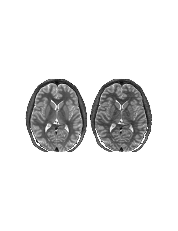
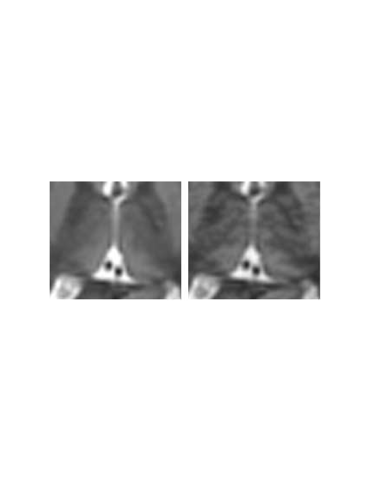
7.2.2 Silhouette-driven k-means (SDK)
This section contains a description of the clustering technique we use in the SNF algorithm. Our clustering technique is based on the K-Means algorithm (Section 7.1.4) and it includes an extension that automatically finds the number of clusters .
We use the clustering criterion that is known as silhouette [176, 114]. Let be a given clustering result. A silhouette in measures how similar a point is to points in its own cluster compared to points in other clusters. Silhouette values range from to and are computed, for a given clustering result , as follows: for each data point , we denote by the set of points in the cluster in that belongs to and by the number of points in the cluster. We define
| (7.3) |
to be the average distance from point to all other points in its cluster in . Let
| (7.4) |
be the minimal average distance from a point to all points in other clusters in . Using Eqs. 7.3 and 7.4, the silhouette value of data point is defined as
| (7.5) |
The silhouette values (derived in Eq. 7.5) of all of the data points can be used as a criterion for assessing the clustering result . Figure 7.3 shows a comparison between two plots of the silhouette values of two clustering results of the same data for two different values of . These plots indicate which clustering result is better.
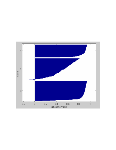 |
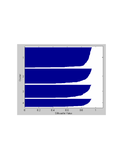 |
Left: a silhouette plot of the result from clustering a data into clusters. The first and the third clusters have large silhouette values (most of them are grater than 0.8), indicating these clusters are well separated from neighboring clusters. The second cluster has relatively low silhouette values (some of them are negative), indicating this cluster is not well separated. The mean across the silhouette values of this clustering result is 0.72.
Right: a silhouette plot of the result from clustering the same data into clusters. All four clusters have large silhouette values (most of them are grater than 0.8), indicating these clusters are well separated. The mean across the silhouette values of this clustering result is 0.86.
The two silhouette plots (left and right) and the mean silhouette values indicate that the clustering result for (right) is better than the one for (left).
In the following, we describe our Silhouette-Driven K-means (SDK) algorithm. In the SDK algorithm, we search for a as large as possible, which produces a clustering with satisfying silhouette values compared to other ’s. The inputs to the algorithm are , and , where is the data points, is a threshold and is a maximal expected number of clusters that depends on the examined data and is usually known a-priori. For instance, for the thalamus, we use a maximum value of , which is based on known results regarding the number of its sub-nuclei (Section 7.1.2). For each , we run K-Means(, ) on the data and compute the mean across the silhouette values of the clustering result. Next, we find that produces the maximal mean silhouette value. Then, we search for the largest that gives a mean silhouette value, that when multiplied by , is larger than the mean silhouette value for . Algorithm 7.1 formulates the SDK algorithm.
SDK(, , )
7.3 The Sub-Nuclei Finder (SNF) algorithm
This section describes our algorithm for sub-nuclei segmentation. The input to the algorithm is a multi-contrast MRI data. This type of data is described in Section 7.1.2 and the specific experimental data that is being used in our work is given in Section 7.4.1. In addition to the multi-contrast MRI values, we also use spatial information. This means that three additional coordinates are added to each features vector, representing the location of the voxel (a voxel is a pixel in a 3D image cube) in the 3D brain space. The spatial information is added since each sub-nuclei is continuous by definition. It implies that neighboring voxels are more likely to belong to the same sub-nucleus than distant ones. The contribution of the spatial coordinates to the feature vector is regulated by a weight coefficient. The output of the algorithm is a mapping of each voxel to its sub-nuclei cluster. In the following we provide a list with the notation that are used for the description of the SNF algorithm.
Notation:
| - | number of slices in the multi-contrast MRI data | |
| - | a slice in the multi-contrast MRI data, ( can also be considered as the z-axis in the 3D brain space) | |
| - | number of contrast acquisition-methods | |
| - | a contrast acquisition-method, | |
| - | 2D image of slice acquired using the contrast acquisition-method | |
| - | 3D image consists of all the 2D images , piled one over the other | |
| - the input data which is received from the multi-contrast MRI acquisition | ||
| - | image after enhancement | |
| - | 3D image that contains all the 2D images , , piled one over the other | |
| and | - | width and height of a slice, respectively |
| and | - | and coordinates of a pixel in the image , respectively, , |
| - the value of contrast acquisition-method (feature) in position | ||
| - a -feature vector of a 3D brain111The feature space is not a 3D space but a space of dimensions, where each point in this dimensional space represents the features acquired by the multi-contrast MRI for each point of the 3D space of the brain. point defined by | ||
| - the set of points in the feature space of dimension , defined by | ||
| - | the set of 3D brain points which belong to the Region of Interest (ROI) | |
| - the set of points from , whose related 3D brain points belong to the ROI | ||
| - | a desired accuracy of the dimensionality reduction process, (see Section 3.5) | |
| - | a factor that controls the influence of the spatial information in respect to the contrast information, | |
| - | a threshold for the SDK algorithm (Algorithm 7.1), | |
| - | maximal expected number of clusters (Section 7.2.2) | |
| - | clustering result |
The SNF algorithm consists of two steps. In the first step, we locate our ROI - region of interest - in the 3D brain space (Section 7.3.1). In the second step, we segment the data that belongs to the ROI into its sub-nuclei in the 3D brain space (Section 7.3.2), using the input data and the ROI information.
A summary of the SNF algorithm is given in Algorithm 7.2. is the input data received from the multi-contrast MRI acquisition. , and are parameters that are empirically chosen. is the maximal expected number of clusters, which is usually known a-priori (Section 7.2.2).
SNF(, , , , )
7.3.1 ROI extraction
This section describes the procedure of locating the ROI in the 3D brain space. It is a semi-automatic procedure, which involves basic expert knowledge.
First, we apply the DB algorithm (Section 4) on the full input data (cube) to reduce its dimensionality. Next, we add the spatial information to the dimension-reduced data, i.e. we attach to each voxel its 3D position in the brain. We multiply the x, y and z coordinates by a scalar to control their influence and append the result as extra coordinates to the feature vector of the voxel. Then, we apply the K-Means algorithm (Section 7.1.4) to the new set of feature vectors to produce a coarse segmentation of the brain into clusters. The number is empirically chosen to separate the ROI from the rest of the data. Large will cause an undesirable phenomenon in which the ROI is divided into separate clusters. Figure 7.4 demonstrates a good separation of the thalamus ROI. Finally, an expert locates the ROI using the produced segmentation to construct the ROI mask. The ROI does not have to appear in all of the slices, e.g. in the data that is used in Section 7.4, the thalamus ROI appears only in slices 22-34.
The functional-flow of the ROI extraction procedure is illustrated in Figure 7.5. The implementation of the ROI extraction procedure is described in Algorithm 7.3.
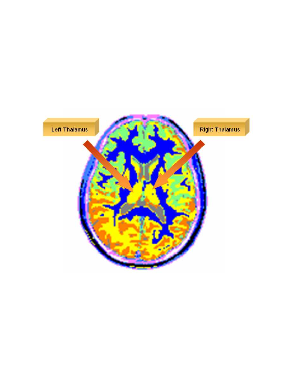
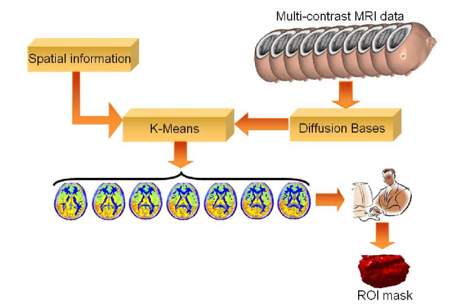
ExtractROI(, , )
-
1.
Construct from , (see notation above)
-
2.
Calculate
-
3.
Calculate () by applying DB on with accuracy , using the Gaussian kernel defined in Eq. 3.1 with from step 2, where , , is the value of the coordinate of the feature vector related to the 3D brain point in the embedding space
-
4.
Add to each vector in the spatial information of its related 3D point in the brain to produce , where , , , , and
-
5.
Calculate =K-Means(, ) (Section 7.1.4), where the number of clusters is empirically chosen
-
6.
For each slice , the ROI is manually marked on the visualization of and its voxels are added to
-
7.
Return
7.3.2 Sub-nuclei segmentation
This section describes the procedure that segments the data, which belongs to the ROI, into sub-nuclei, using the set of points in the feature space and the ROI information. It is a fully automatic procedure and no human intervention is needed. An optional procedure that can follow may allow an expert to manually merge clusters.
First, we apply the wavelet-based image enhancement (Section 7.2.1) on each slice of each contrast acquisition-method. This procedure produces denoised and contrast-improved slices. Since our distance metric is not invariant to scaling, we need to normalize the data. We normalize each enhanced contrast acquisition-method (feature) separately based on its range of values inside the ROI. The normalization procedure is described in Algorithm 7.4. Then, we use the normalized enhanced data, the ROI mask (Section 7.3.1) and the spatial information as the input to the DM procedure (Section 3). The ROI mask is used to select the desired region from the normalized enhanced data. This selected data is combined with the spatial information to be used as an input to the DM procedure. The complexity of the DM procedure is reduced since points which are outside the ROI are excluded. Then, we apply the SDK algorithm (Section 7.2.2) on the dimension-reduced output of the DM algorithm in order to segment the ROI, into its sub-nuclei.
The clustering result contains isolated points, i.e. single-voxel segments that are located inside larger segments. We merge the isolated points using a procedure that is described in Algorithm 7.5, in order to get more homogeneous segments. This is based on the assumption that the nuclei are continuous. Figure 7.6 shows a comparison between the segmentation results before and after the merging of isolated points.
The functional-flow of the sub-nuclei segmentation procedure is illustrated in Figure 7.7. The implementation of the sub-nuclei segmentation procedure is described in Algorithm 7.6.
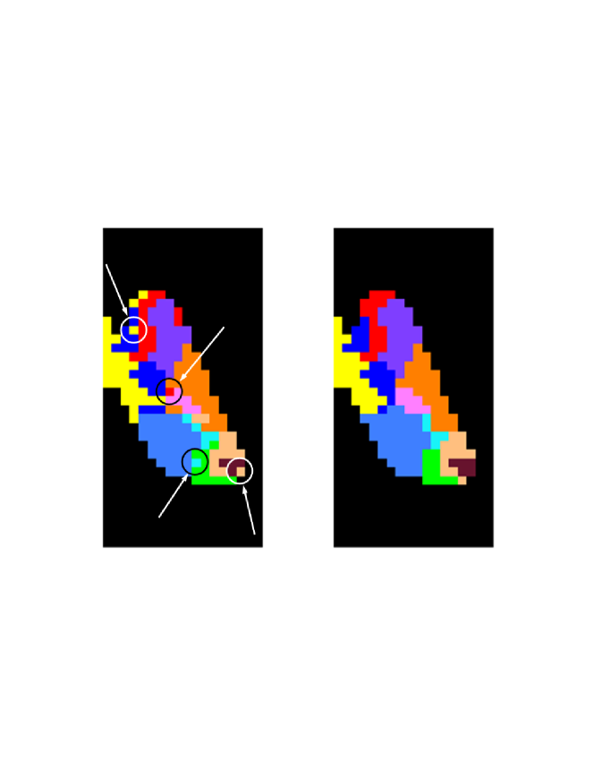
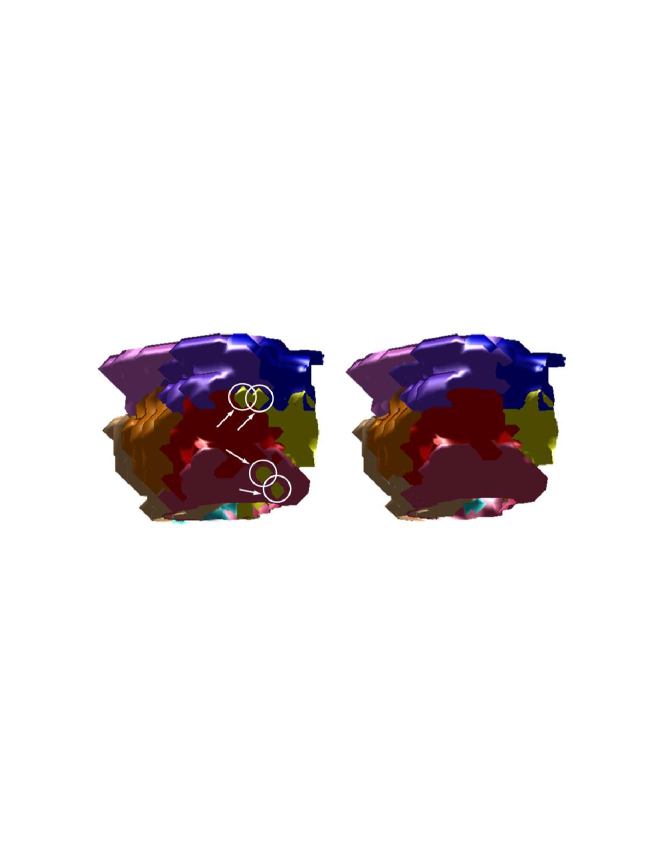
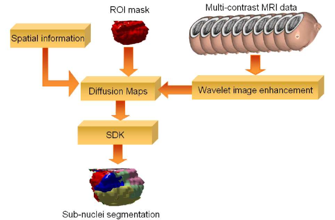
NormalizeContrastMethod(, )
-
1.
Calculate
where and are the mean and the standard deviation values of voxels that belong to the ROI , respectively
-
2.
Transform to be in [0,1] by applying the following mapping
where and are the minimum and the maximum values of voxels that belong to the ROI , respectively
-
3.
Return
MergeIsolatedPoints()
For each slice in do:
-
1.
Search for all the “isolated points” that have less than or exactly one neighbor of the same cluster in its 8-connected neighborhood
-
2.
For every isolated point, search for its closest or containing cluster by searching in its 8-connected neighborhood
-
3.
For every point: if it is an isolated point, transfer it into its most closer cluster, otherwise leave it in its current cluster
Return
SubNucleiSegmentation(, , , , , )
-
1.
Construct , , , from
-
2.
Apply the wavelet-based image enhancement algorithm (Section 7.2.1) on each to produce enhanced images , ,
-
3.
Calculate = NormalizeContrastMethod(, ),
(Algorithm 7.4) -
4.
Construct from , (see notation), where , , is the value of coordinate in the enhanced space of a 3D brain point .
-
5.
Construct from and
-
6.
Add to each vector in the spatial information of its related 3D brain point to produce , where , , , , and
-
7.
Calculate
-
8.
Calculate (’) by applying DM on with accuracy , using the Gaussian kernel defined in Eq. 3.1 with from step 7, where , , is the value of coordinate of the feature vector in the embedded space, related to the 3D brain point
-
9.
Calculate = SDK(, , ) (Algorithm 7.1)
-
10.
Calculate = MergeIsolatedPoints() (Algorithm 7.5)
-
11.
Return
7.4 Experimental results
In this section we present the results after the application of the SNF algorithm (Algorithm 7.2) on a multi-contrast MRI data of a human brain. The goal was to segment the thalamus into its sub-nuclei. Details about the acquisition process of the experimental data are given in Section 7.4.1. Using the ROI extraction procedure of the SNF algorithm (Section 7.3.1) on this data, we were able to detect the thalamus (Figure 7.4). The volume of each detected thalamic part (right and left) was found to be approximately 7050 . Our algorithm detected up to 13 clusters of the right/left thalamus.
The spectrum of a cluster is a vector, whose coordinates represent different contrast-acquisition-method information that is related to the points in this cluster. Specifically, each coordinate contains a value associated with an image from a different (Algorithm 7.4) contrast acquisition-method after normalization. A coordinate value is the median across the values of the pixels that are associated with the points of the cluster which were obtained from the relevant contrast acquisition-method after normalization. The values of the spectrum are ordered according to their appearance in Table 7.2. In the following, we formulate the calculation of a spectrum for a given cluster.
Let be a cluster. For each point , , let be the coordinates of in the 3D space of the brain and let be the value of the pixel obtained by contrast acquisition-method after normalization at point , (see Section 7.3 for notation and Algorithm 7.4 for the normalization process). The spectrum of is defined as
| (7.6) |
The values of the coordinates of are in the range of [0,1].
Some of the clusters significantly differ in their spectrum, supporting the hypothesis that nuclei can be separated by their multi-contrast data. Figure 7.8 presents two dissimilar spectra of two different clusters.
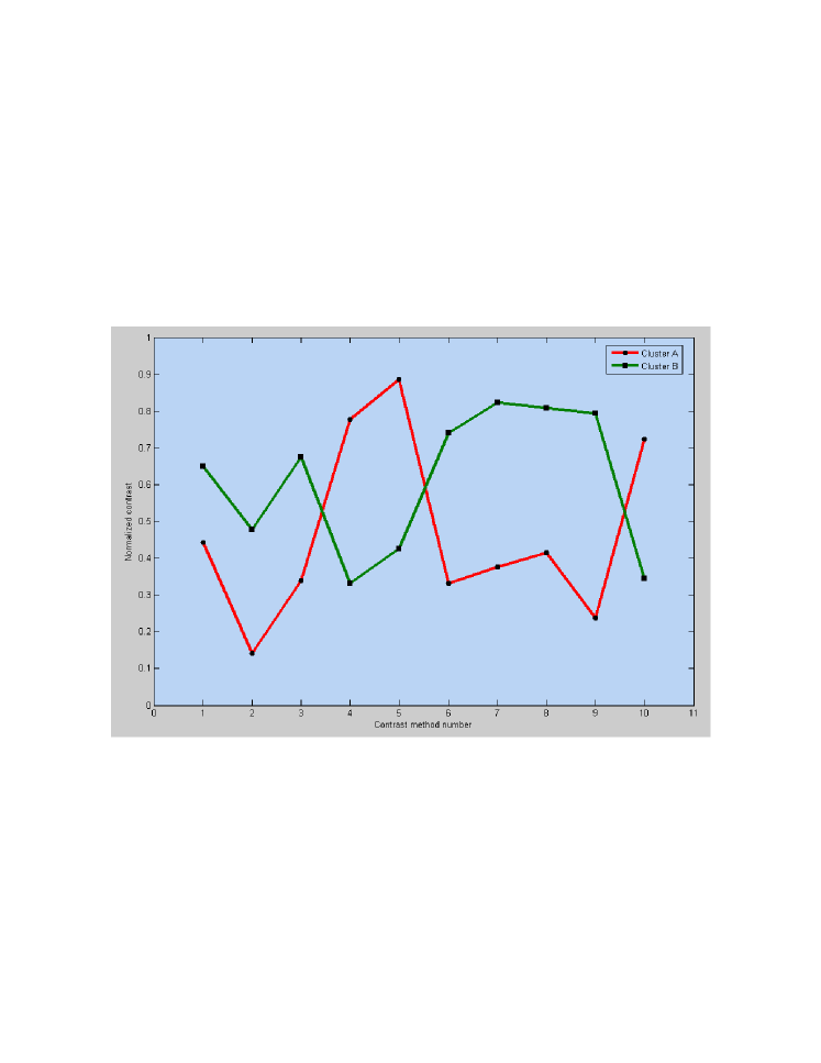
Due to the variability that exists in the nuclei shapes, sizes and locations in the brain of each individual (Section 7.1.1), there is no agreeable measurement that we can use to evaluate the performance of the SNF algorithm. A combination of inter-subject variability and utilization of different types of histological methods is the cause for variability among different histological atlases. Figure 7.9 gives a visual demonstration of this phenomenon. It shows the same slice from two different atlases, colored according to the sub-nuclei arrangement. The sub-nuclei in one atlas differ from their counterparts in the second atlas in their geometric characteristics (shape, size and location).
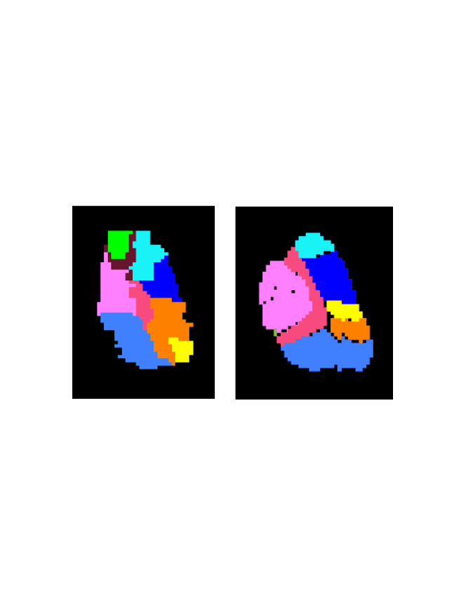
Therefore, we measure the quality of the outputs from the SNF algorithm by:
-
•
comparing the detected nuclei locations to a histological atlas in Section 7.4.2
-
•
matching between subjects in Section 7.4.3
-
•
matching between the left and the right parts of the thalamus of the same subject in Section 7.4.4.
In Section 7.4.5 we demonstrate the contribution of the image enhancement and the dimensionality reduction procedures in the SNF algorithm. We do this by comparing the results produced using versions of the SNF algorithm that exclude each of these procedures, to the results produced using the full SNF algorithm, as defined in Algorithm 7.2. Finally, in Section 7.4.6, we summarize the experimental results.
7.4.1 The experimental data
We tested our algorithm on a number of multi-contrast MRI data. The data was acquired using a 3T GE 8-channel head coil MRI scanner. The scans are of nine healthy males aged 25 to 30. Each subject was scanned with ten different contrasts (, see notation in Section 7.3), which were achieved by variation of acquisition parameters such as time to repeat and time to echo. Table 7.2 describes the values of the parameters that were used for each contrast acquisition-method.
| # | Contrast Acquisition-Method | Time to repeat () | Time to echo () | Experiment time () | Extra information |
|---|---|---|---|---|---|
| 1 | FLAIR | 9000 | 140 | 4:50 | Time to invert = 2100 ms |
| 2 | T2 weighted | 7000 | 150 | 3:00 | Echo train length = 32 |
| 3 | Proton Density | 7000 | 6 | 3:00 | Echo train length = 32 |
| 4 | T1 weighted | 550 | 8 | 5:00 | |
| 5 | T1 + MgT | 550 | 8 | 6:20 | Irradiation frequency = 1.2 kHz |
| 6 | T2 short TE | 600 | 2 | 5:00 | Flip Angle = |
| 7 | T2 medium TE | 600 | 15 | 5:00 | Flip Angle = |
| 8 | T2 long TE | 600 | 32 | 5:00 | Flip Angle = |
| 9 | STIR | 5000 | 25 | 3:00 | Time to invert = 130 |
| 10 | SPGR | 400 | 2 | 2:30 | Flip Angle = |
FLAIR: Fluid Level Attenuated Inversion Recovery, MgT: Magnetization Transfer, STIR: Short Tau Inversion Recovery, SPGR: Spoiled Gradient Recalled Echo.
Each specific contrast scan produced 48 images made in the axial plane with a Field of View (FOV) of . Each image represents a slice, 1.5 thick, with no gaps and contains pixels with spatial resolution of 1.5 in both axes. Hence, the scanning provides a 3D resolution of . After the scanning phase, the various contrast images, which belong to the same subject and to the same slice, were realigned in order to correct head motion corrections. In addition, for comparison reasons, all subjects volumes were co-registered and re-sliced to a single chosen subject. Figures 7.10-7.13 give a visual illustration of the variability between the different contrast acquisition-methods. Figures 7.10, 7.11 and 7.12 show the values of the ten resulted contrasts of the thalamus ROI for a specific slice of one of the subjects. Figure 7.13 shows the ten contrast images (one for each contrast acquisition-method) for a specific slice of one of the subjects.
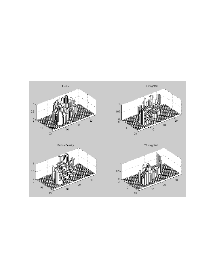
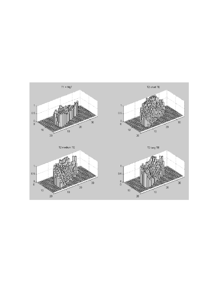
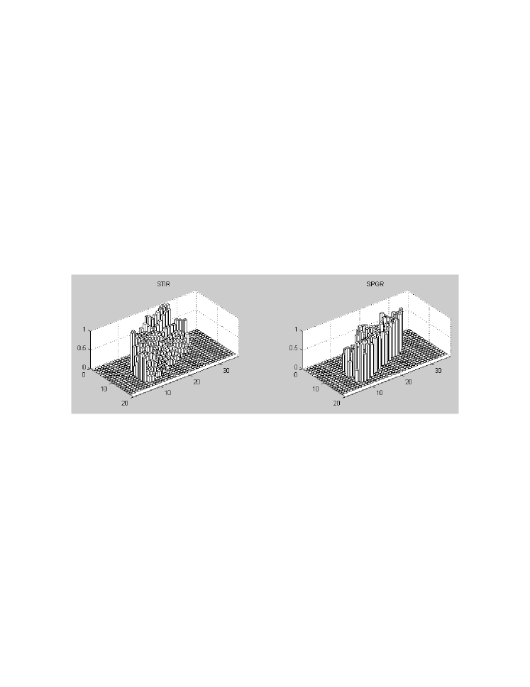
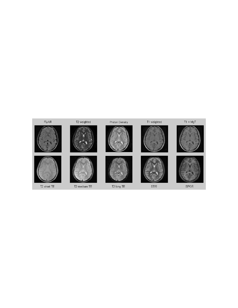
7.4.2 Matching to histological atlas
In order to evaluate the results of the SNF algorithm (Algorithm 7.2) applied on the multi-contrast MRI data, we compare them to a histological atlas. We apply the SNF algorithm on the data that belongs to one of the nine subjects from Section 7.4.1. We use the atlas of Kikinis [116] for the comparison.
The atlas is first digitized and registered to the subject. Each voxel of the atlas is labeled according to the nucleus it belongs to. After labeling the atlas voxels, we compute the centroids of each labeled cluster in the 3D space. In addition, we compute the centroids of the clusters produced by the SNF algorithm on the subject. Then, we calculate in the common 3D space the distances between the centroids of the subject and the centroids of the atlas. We define the distance between two clusters as the distance between their centroids. Every cluster of the subject is assigned the label of the cluster in the atlas that is closest to it. This process may assign the same label to two or more different clusters. This phenomenon is acceptable for the sake of comparison and it indicates that the segmentation separates the data into more sub-nuclei than the ones in this specific atlas.
The geometric characteristics (shape, size and location) of the matched segmented nuclei were consistent with the registered atlas. The mean distance error from the segmented nuclei centroids to their matched atlas nuclei centroids was 2.8 (while the total volume of the right thalamus was found to be 7,043 ). A perfect match is not feasible due to the inter-subject variability (Section 7.1.1) and the imperfect registration. Figure 7.14 shows a single slice from the result of a match between the atlas and the output of the SNF algorithm applied on the data of the right thalamus of one of the subjects. Figure 7.15 shows some 3D views of this match. There is high resemblance between the geometric characteristics of the matched nuclei and the geometric characteristics of their counterparts in the atlas.
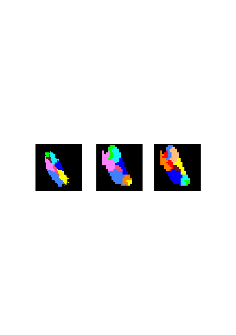
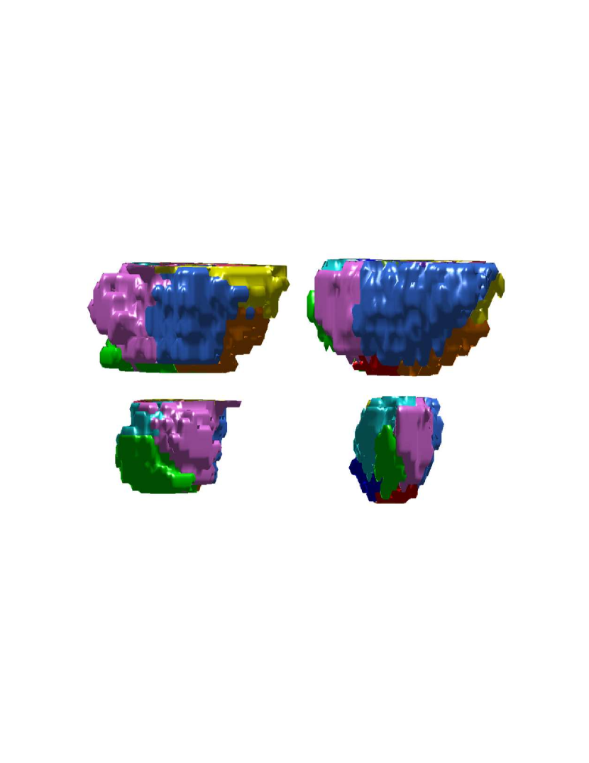
7.4.3 Match between subjects
We further examine the performance of the SNF algorithm (Algorithm 7.2) by comparing between the results it produced for different subjects. We used the same matching technique that was presented in Section 7.4.2. Figure 7.16 shows a single slice from the result of a match between the outputs of the SNF algorithm applied on the data of the right thalami of two different subjects. Figure 7.17 shows a 3D view of this match. There is a certain resemblance between the geometric characteristics (shape, size and location) of the matched nuclei, despite the inter-subject variability (Section 7.1.1). The mean distance error between the matched centroids was 3.55 . Figure 7.18 shows the matched centroids in the 3D brain space. It shows the matching errors that are due to the imperfect match.
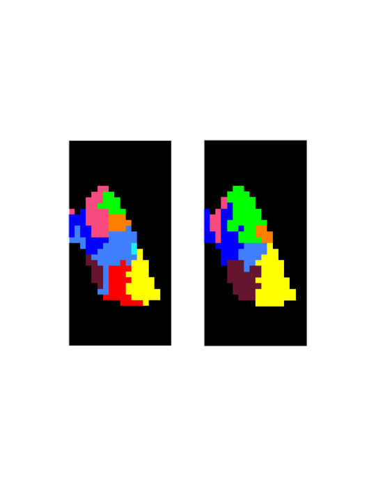
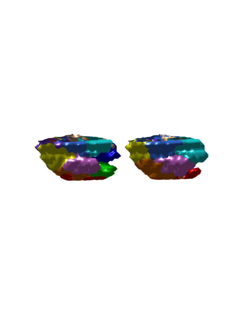
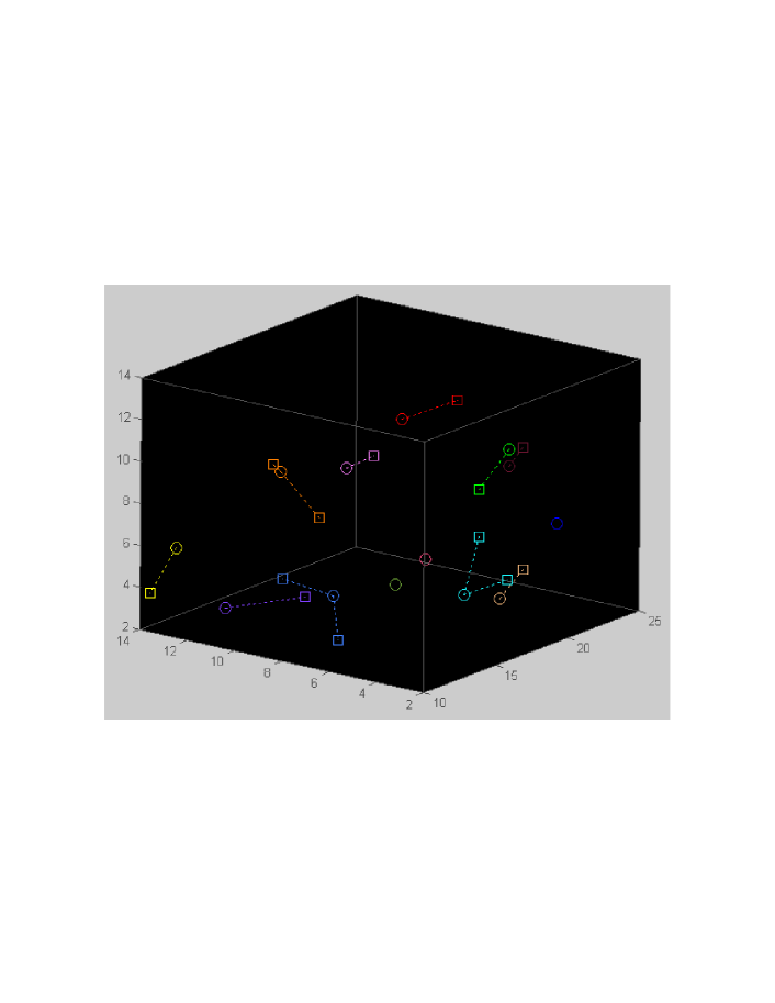
We also examined the spectra (Eq. 7.6) of the matched clusters. Figure 7.19 illustrates the high resemblance between the spectra of two matched clusters from two different subjects.
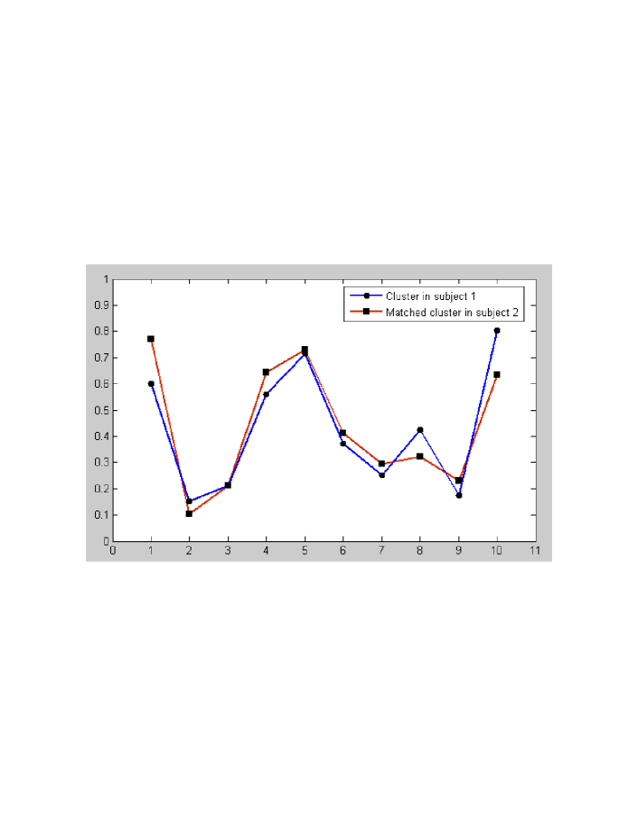
7.4.4 Matching between the two parts of the thalamus
In order to further evaluate and validate the output of the SNF algorithm (Algorithm 7.2), we take advantage of the fact that the left part and the right part of the thalamus are similar (Figure 7.4). We applied the SNF algorithm separately on each of these thalamus parts of a subject. The output from the right part to resembles the output from the left part. We use the matching technique that was presented in Section 7.4.2 to evaluate the similarity. The matching technique used a mirror image of the left part of the thalamus. Figure 7.20 demonstrates the matching between the outputs of the SNF algorithm applied on the data of the two thalamus parts of the same subject. Figure 7.21 shows a 3D view of this match. There is a resemblance between the geometric characteristics (shape, size and location) of the matched nuclei. However, it is not a perfect match since the thalamus right and left parts are not identical.

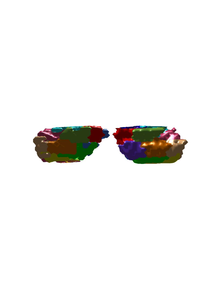
To achieve better accuracy, a more advanced registration technique is needed to register the left part and the right part since there is not a perfect match between their shapes. The mean distance error between matched centroids was 4.14 . Figure 7.22 illustrates high resemblance between two spectra that belong to two matched clusters: one cluster is part of the output of the SNF algorithm applied on the left side of the thalamus of a subject and the other cluster is part of the output of the SNF algorithm applied on the right side of the thalamus of the same subject.
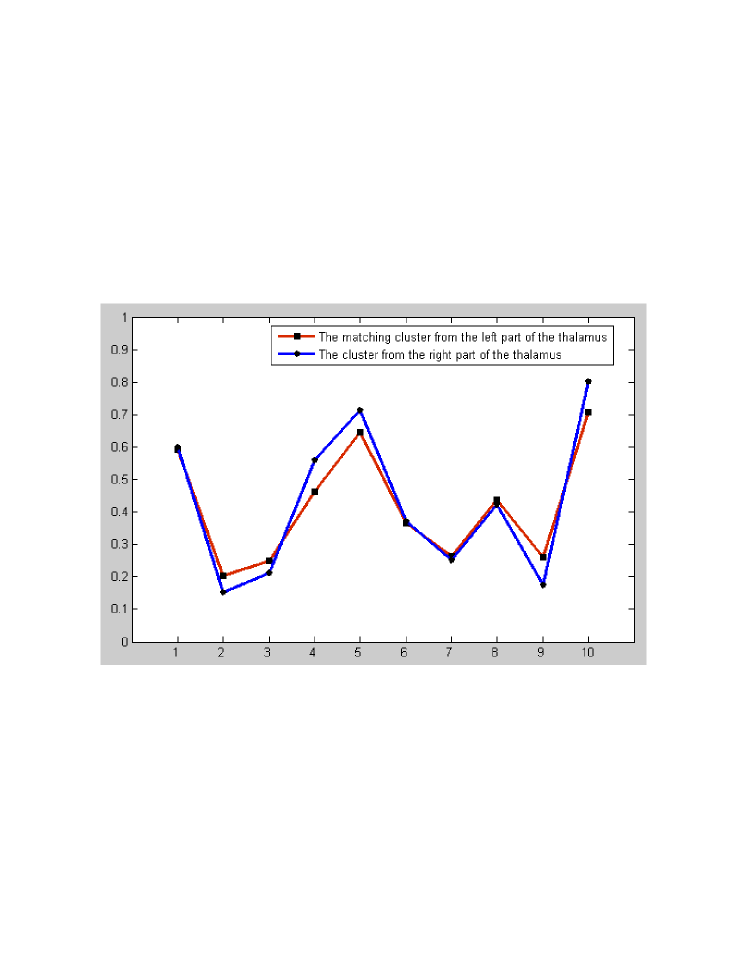
We also apply the SNF algorithm on the whole thalamus area, i.e. on the ROI that includes both the left and the right parts of the thalamus. The result is depicted in Fig. 7.23. Matched clusters from the left part and the right part are not necessarily colored in the same color since they were discovered as different clusters due to the use of the spatial information.

7.4.5 Contribution of the main steps of the SNF algorithm
In this section we show the benefits of using the image enhancement and the dimensionality reduction steps of the SNF algorithm. Following are some comparisons between results of the SNF algorithm using all its steps (we refer to this version as the full SNF algorithm) and results of the SNF algorithm where each of these steps is excluded (we refer to these versions as the partial SNF algorithms).
Image enhancement
We exclude the image enhancement procedure from the SNF algorithm and apply it on the same subject that was examined in Section 7.4.2. The results were poor in comparison with the results of the full SNF algorithm. The partial SNF algorithm detected only 6 clusters in the right thalamus that were matched to 5 nuclei of the atlas, while the full SNF algorithm detected 13 clusters, that were matched to 10 nuclei of the atlas. The superiority of the full SNF algorithm stems from the noise reduction and the non-linear feature amplification mechanism of the wavelet-based image enhancement (Section 7.2.1). Figure 7.24 illustrates this comparison. The number of sub-nuclei, which were detected by the application of the partial SNF algorithm (excluding the image enhancement step), is less than the number of sub-nuclei, that were detected by the application of the full SNF algorithm (including the image enhancement step). Moreover, a comparison between the geometric characteristics (shape, size and location) of the detected nuclei (by both algorithm versions) and their counterparts in the atlas, reveals that the result of the full SNF algorithm bares a stronger similarity to the atlas.
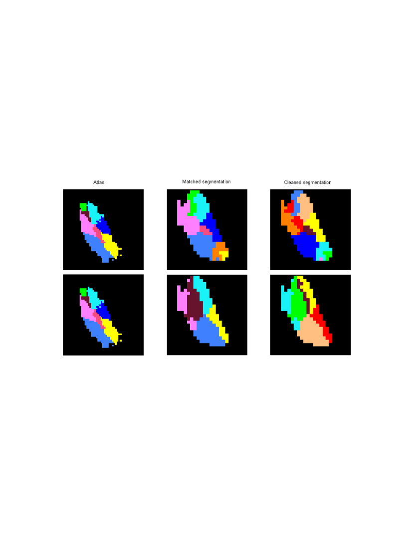
Dimensionality reduction
We exclude the dimensionality reduction phase from the SNF algorithm and apply it on the data of the same subject that we examined in Section 7.4.2. There was substantial degradation in the quality of the results: the partial SNF algorithm detected only 10 clusters in the right thalamus, that were matched to 8 nuclei in the atlas, while the full SNF algorithm detected 13 clusters, that were matched to 10 nuclei in the atlas. Figure 7.25 illustrates this comparison. The number of sub-nuclei, which were detected by the partial SNF algorithm (excluding the dimensionality reduction step), is less than the number of sub-nuclei, which were detected by the full SNF algorithm (including the dimensionality reduction step). Moreover, a comparison between the geometric characteristics (shape, size and location) of the detected nuclei (by both algorithm versions) and their counterparts in the atlas, reveals a better similarity to the output of the full SNF algorithm.
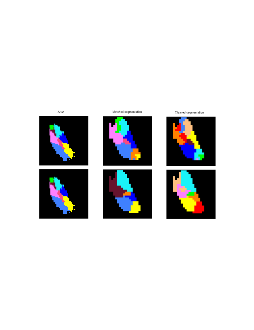
Furthermore, the time complexity of the partial SNF algorithm was much higher in comparison to that of the full SNF algorithm: 170 versus 106 on a Pentium4 2.4 with 768 RAM. This is due to the clustering procedure, whose time complexity significantly grows with increase of the dimensionality of the data.
We also investigated the performance of the dimensionality reduction process we use in Algorithm 7.6, which is based on the DM framework (Chapter 3), to the classical dimensionality reduction technique - PCA (Section 2.1). We used PCA instead of the DM for the dimensionality reduction step and kept the same number of eigenvectors in both the PCA process and the DM process. As expected, the time complexity was reduced from 106 (using DM) to 75 (using PCA) since PCA has a lower complexity than local non-linear methods (Section 2.2). However, the results of the PCA-based SNF algorithm were inferior to those of the DM-based SNF algorithm (the original SNF algorithm). The PCA-based SNF algorithm managed to detect only 7 clusters in the right thalamus that were matched to 6 nuclei of the atlas, while the DM-based SNF algorithm detected 13 clusters that were matched to 10 nuclei of the atlas. Moreover, the mean distance error between the segmented nuclei centroids to their matched atlas nuclei centroids was 3.53 in the PCA-based SNF algorithm outputs, while in the DM-based SNF algorithm outputs this value was 2.8 (Section 7.4.2). Figure 7.26 illustrates this comparison. Figure 7.27 shows a 3D view of the compared results. The number of sub-nuclei, that were detected by the application of the PCA-based SNF algorithm, is less than the number of sub-nuclei, which were detected by the application of the DM-based SNF algorithm. Moreover, a comparison between the geometric characteristics (shape, size and location) of the detected nuclei (by both algorithm versions) and their counterparts in the atlas, reveals a better similarity to the output of the DM-based SNF algorithm. Furthermore, the DM-based SNF algorithm detected sub-nuclei that are geometrically smoother than those that were detected by the PCA-based SNF algorithm.
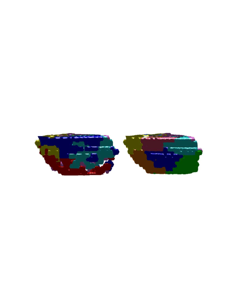
7.4.6 Summary of results
Tables 7.3 and 7.4 summarize the experimental results. Table 7.3 summarizes the results of evaluating the SNF algorithm applied on different types of data. In all cases, there was a good match between the number of nuclei of the two examined objects: subject and atlas, two subjects and the two parts of the thalamus. Specifically, 10 out of the 13 nuclei were shown to match. The visual match between the results is very high for the subject and atlas. This is corroborated by a low matched centroids mean distance error (). The results for the two subjects and the two part of thalamus are also good however, they are inferior to those of the subject and atlas. Table 7.4 summarizes the results of evaluating different versions of the SNF algorithm applied on the same data.
| Criterion |
|
|
|
||||||
|---|---|---|---|---|---|---|---|---|---|
| visual resemblance | very high | high | medium | ||||||
| number of detected clusters | 13 | 13 | 13 | ||||||
| number of matched clusters | 10 | 10 | 10 | ||||||
| matched centroids mean distance error () | 2.8 | 3.55 | 4.14 |
| Criterion |
|
|
|
|
||||||||
|---|---|---|---|---|---|---|---|---|---|---|---|---|
| visual resemblance to atlas | very high | medium | medium | medium | ||||||||
| number of detected clusters | 13 | 6 | 10 | 7 | ||||||||
| number of matched clusters | 10 | 5 | 8 | 6 | ||||||||
| running time () | 106 | 76 | 170 | 75 |
7.5 Conclusion and future work
In this chapter, we introduced a novel algorithm (the SNF algorithm) for automatic segmentation of neuronal tissue into its sub-nuclei. By using an in-vivo multi-contrast MRI data of a human brain as an input, we achieved a good segmentation of the thalamus into its sub-nuclei. Namely, the SNF algorithm automatically identified the major nuclei of the thalamus. The results of the SNF algorithm were found to strongly agree with a known histological atlas [116]. Moreover, the outputs were found to be consistent for different subjects and for the two parts of the thalamus of the same subject222in both cases up to inner-subject variability..
The results of the algorithm can be improved by a better selection of the input data. For instance, one should perform an in-vitro333Since the desired acquisition time is too long to perform in-vivo and to allow a histological examination. experiment, that includes acquisition of a large number of different contrast acquisition-methods in higher resolution. Then, after the application of the SNF algorithm on the contrast acquisition-methods, the spectra of the clusters should be examined to identify a reasonable number of contrast acquisition-methods, that give the best separation, when combined together. Furthermore, an in-vitro histological-based sub-nuclei segmentation of the examined sample should be performed, in order to validate the results. Then, the identified contrast acquisition-methods should be used in-vivo. The described technique should produce a more accurate segmentation (separation into smaller nuclei) than the segmentation by histological methods.
Chapter 8 Video Segmentation via Diffusion Bases
Identifying moving objects in a video sequence, which is produced by a static camera, is a fundamental and critical task in many computer-vision applications. A common approach performs background subtraction and thus identifies moving objects as the portion of a video frame that differs significantly from a background model. A good background subtraction algorithm has to be robust to changes in the illumination and it should avoid detecting non-stationary background objects such as moving leaves, rain, snow, and shadows. In addition, the internal background model should quickly respond to changes in background such as objects that start to move or stop.
In this chapter, we present a new algorithm for video segmentation that processes the input video sequence as a 3D matrix where the third axis is the time domain. Our approach identifies the background by reducing the input dimension using the diffusion bases methodology. Furthermore, we describe an iterative method for extracting and deleting the background. The algorithm has two versions and thus covers the complete range of backgrounds: one for scenes with static backgrounds and the other for scenes with dynamic (moving) backgrounds.
8.1 Introduction
Video surveillance systems, tracking systems, imaging-based statistical packages that count people, games, etc. seek to automatically identify people, objects, or events of interest in different environment types. Typically, these systems consist of stationary cameras, that are directed at offices, parking lots, playgrounds, fences and so on, together with computer systems that process the video frames. Human operators or other processing elements are notified about salient events. There are many needs for automated surveillance systems in commercial, law enforcement, and military applications. One possible application is a continuous 24-hour monitoring of surveillance video to alert security officers of a burglary in progress or a suspicious individual loitering in a parking lot.
In addition to the obvious security applications, video surveillance technology has been proposed to measure traffic flow, detect accidents on highways, monitor pedestrian congestion in public spaces, compile consumer demographics in shopping malls and amusement parks, log routine maintenance tasks at nuclear facilities, and count endangered species. The numerous military applications include patrolling national borders, measuring the flow of refugees in troubled areas, monitoring peace treaties, and providing secure perimeters around bases.
A common element in surveillance systems is a module that performs background subtraction to distinguish between background pixels, which should be ignored, and foreground pixels, which should be processed for identification or tracking. The difficulty in background subtraction is not to differentiate, but to maintain the background model, its representation and its associated statistics. In particular, capturing the background in frames where the background can change over time. These changes can be moving trees, leaves, water flowing, sprinklers, fountains, video screens (billboards) just to name a few typical examples. Other forms of changes are weather changes like rain and snow, illumination changes like turning on and off the light in a room and changes in daylight. We refer to this background type as dynamic background (DBG) while a background that slightly changes or does not change at all is referred to as static background (SBG).
Subtraction of backgrounds, which are captured by static cameras, is also useful to achieve low-bit rate video compression for transmission of rich multimedia content. The subtracted background is transmitted once, followed by the segmented objects which are detected.
In this chapter, we present a new method for capturing the background. It is based on the application of the diffusion bases (DB) algorithm (Chapter 4). Moreover, we introduce a real time iterative method for background subtraction in order to separate between background and foreground pixels while overcoming the presence of changes in the background. The main steps of the algorithm are:
-
•
Extract the background frame by dimensionality reduction via the application of the DB algorithm.
-
•
Subtract the background from the input sequence.
-
•
Threshold the subtracted sequence.
-
•
Detect the foreground objects by applying depth first search (DFS) on a graph model of the background-subtracted sequence.
We propose two versions of the algorithm - one for static background and the other for dynamic background. To handle dynamic background, a learning process is applied to data that contains only the background objects in order to construct a frame that will contain the DBG to be extracted. The proposed algorithm outperform current state-of-the-art algorithms.
The rest of this chapter is organized as follows: in Section 8.2, related algorithms for background subtraction are presented. The main algorithm, that is called the background subtraction algorithm using diffusion bases (BSDB), is presented in Section 8.3. In Section 8.4, we present experimental results, a performance analysis of the BSDB algorithm and we compare it to other background subtraction algorithms.
8.2 Related work
Background subtraction is a widely used approach for detection of moving objects in video sequences that are captured by static cameras. This approach detects moving objects by differentiating between the current frame and a reference frame, often called the background frame, or background model. In order to extract the objects of interest, a threshold can be applied to the subtracted frame. The background frame should faithfully represent the scene. It should not contain moving objects. In addition, it must be regularly updated in order to adapt to varying conditions such as illumination and geometry changes. This section provides a review of the current state-of-the-art background subtraction techniques. These techniques range from simple approaches, aiming to maximize speed and minimizing the memory requirements, to more sophisticated approaches, aiming to achieve the highest possible accuracy under any possible circumstances. The goal of these approaches is to run in real-time. Additional references can be found in [140, 168, 142].
-
•
Temporal median filter: In [141], is was proposed to use the median value of the last frames as the background model. This provides an adequate background model even if the frames are subsampled with respect to the original frame rate by a factor of 10 [54]. The median filter is computed on a special set of values that contains the last subsampled frames and the last computed median value. This combination increases the stability of the background model [54].
The main disadvantage of a median-based approach is that its computation requires a buffer with the recent pixel values. Furthermore, no deviation measure was provided with which the subtraction threshold can be adapted. -
•
Gaussian average: This approach models the background independently at each pixel location [232]. The model is based on ideally fitting a Gaussian probability density function (pdf) to the last pixels. At each new frame at time , a running average is computed by where is the current frame, is the previous average and is an empirical weight that is often chosen as a trade-off between stability and quick update.
In addition to speed, the advantage of the running average is given by a low memory requirement. Instead of a buffer with the last pixel values, each pixel is classified using two parameters , where is the standard deviation. Let be the pixel at time . is classified as a foreground pixel if . Otherwise is classified as background pixel. -
•
Mixture of Gaussians: In order to cope with rapid changes in the background, a multi-valued background mode was suggested in [203]. In this model, the probability of observing a certain pixel at time is represented by a mixture of Gaussians distributions: where for each -th Gaussian in the mixture at time , estimates what portion of the data is accounted for by this Gaussian, is the mean value, is the covariance matrix and is a Gaussian probability density function. In practice, is set to be between 3 and 5. Each of the Gaussian distributions describes only one of the observable background or foreground objects. The distributions are ranked according to the ratio between their peak amplitude and their standard deviation . Let be the threshold value. The first distributions that satisfy are accepted as background. All the other distributions are considered as foreground.
Let be a frame at time . At each frame , two events take place simultaneously: assigning the new observed value to the best matching distribution and estimating the updated model parameters. The distributions are ranked and the first that satisfies is a match for . -
•
Kernel density estimation (KDE): This approach models the background distribution by a non-parametric model that is based on a Kernel Density Estimation (KDE) of the buffer of the last n background values ([71]). KDE guarantees a smooth, continuous version of the histogram of the most recent values that are classified as background values. This histogram is used to approximate the background pdf.
The background pdf is given as a sum of Gaussian kernels centered at the most recent background values, : where is the kernel estimator function and represents the kernel function bandwidth. is estimated by computing the median absolute deviation over the sample for consecutive intensity values of the pixel. Each Gaussian describes just one sample data. The buffer of the background values is selectively updated in a FIFO order for each new frame .
In this application two similar models are concurrently used, one for long-term memory and the other for short-term memory. The long-term model is updated using a blind update mechanism that prevents incorrect classification of background pixels. -
•
Sequential kernel density approximation: Mean-shift vector techniques have been employed for various pattern recognition problems such as image segmentation and tracking ([49, 50]). The mean-shift vector is an effective technique capable of directly detecting the main modes of the pdf from the sample data using a minimum set of assumptions. However, it has a very high computational cost since it is an iterative technique and it requires a study of the convergence over the whole data space. As such, it is not immediately applicable to modeling background pdfs at the pixel level.
To solve this problem, computational optimizations are used to mitigate the computational high cost ([169]). Moreover, the mean-shift vector can be used only for an off-line model initialization [88], i.e. the initial set of Gaussian modes of the background pdf is detected from an initial sample set. The real-time model is updated by simple heuristics that handle mode adaptation, creations, and merging. -
•
Co-occurrence of image variations: This method exploits spatial co-occurrences of image variations ([194]). It assumes that neighboring blocks of pixels that belong to the background should have similar variations over time. The disadvantage of this method is that it does not handle blocks at the borders of distinct background objects.
This method divides each frame to distinct blocks of pixels where each block is regarded as an -component vector. This trades-off resolution with high speed and better stability. During the learning phase, a certain number of samples is acquired at a set of points, for each block. The temporal average is computed and the differences between the samples and the average, called the image variations, is calculated. Then the covariance matrix is computed with respect to the average. An eigenvector transformation is applied to reduce the dimensions of the image variations.
For each block , a classification phase is performed: the corresponding current eigen-image-variations are computed on a neighboring block of . Then the image variation is expressed as a linear interpolation of its L-nearest neighbors in the eigenspace. The same interpolation coefficients are applied on the values of , to provide an estimate for its current eigen-image-variations. -
•
Eigen-backgrounds: This approach is based on an eigen-decomposition of the whole image [162]. During a learning phase, samples of images are acquired. The average image is computed and subtracted from all the images. The covariance matrix is computed and the best eigenvectors are stored in an eigenvector matrix. For each frame , a classification phase is executed: is projected onto the eigenspace and then projected back onto the image space. The output is the background frame, which does not contain any small moving objects. A threshold is applied on the difference between and the background frame.
8.3 The Background Subtraction Algorithm using Diffusion Bases (BSDB)
In this section we present the BSDB algorithm. The algorithm has two versions:
Static background subtraction using DB (SBSDB)
We assume that the background is static (SBG) – see Section 8.3.1. The video sequence is captured on-line. Gray level images are sufficient for the processing.
Dynamic background subtraction using DB (DBSDB)
We assume that the background is moving (DBG) – see Section 8.3.2. This algorithm uses off-line (training) and on-line (detection) procedures. As opposed to the SBSDB, this algorithm requires color (RGB) frames.
Both algorithms assume that the camera is static.
8.3.1 Static background subtraction algorithm using DB (SBSDB)
In this section we describe the on-line algorithm that is applied on a video sequence that is captured by a static camera. We assume that the background is static. The SBSDB algorithm captures the static background, subtracts it from the video sequence and segments the subtracted output.
The input to the algorithm is a sequence of video frames in gray-level format. The algorithm produces a binary mask for each video frame. The pixels in the binary mask that belong to the background are assigned 0 values while the other pixels are assigned to be 1.
8.3.1.1 Off-line algorithm for capturing static background
In order to capture the static background of a scene, we reduce the dimensionality of the input sequence by applying the DB algorithm (see Chapter 4). The input to the algorithm consists of frames that form a datacube.
Formally, let
| (8.1) |
be the input datacube of frames each of size where is the pixel at position in the video frame at time . We define the vector to be the values of the coordinate at all the frames in . This vector resembles a hyper-pixel (see Section 6.1) and will be named so from this point on. Let be the set of all hyper-pixels. We define to be a 1-D vector representing the video frame at time . We refer to as a frame-vector. Let be the set of all frame-vectors.
We apply the DB algorithm to by =DiffusionBasis(, , , ) where is defined by Eq. 3.1, the DiffusionBasis procedure was defined in algorithm 4.1 and , are defined in Section 3.1 and 3.3, respectively (see also Section 3.4 for an algorithm to calculate ). The output is the projection of every hyper-pixel on the diffusion basis which embeds the original data into a reduced space. The first vector of represents the background of the input frames. Let , be this vector. We reshape into the matrix . Then, is normalized to be between 0 to 255. The normalized background is denoted by .
8.3.1.2 On-line algorithm for capturing a static background
In order to make the algorithm suitable for on-line applications, the incoming video sequence is processed by using a sliding window (SW) of size . Thus, the number of frames that are input to the algorithm is . Naturally, we seek to minimize in order to obtain a faster result from the algorithm. We found empirically that the algorithm produces good results for values of as low as and . The delay of 5 to 7 frames is negligible and renders the algorithm suitable for on-line applications.
Let be the input video sequence. we apply the algorithm that is described in Section 8.3.1.1 to every SW. The output is a sequence of background frames
| (8.2) |
where is the background that corresponds to frame and till are set to . Figure 8.1 describes how the SW is shifted.
The SW results in a faster execution time of the DB algorithm. The
weight function (Eq. 3.1) is not
recalculated for all the frame in the SW. Instead,
is only updated according to the new frame that enters the SW and
the one that exits the SW. Specifically, let
be the SW at time and let
be the SW at time . At time , is calculated
only for and the entries that correspond to are
removed from .

8.3.1.3 The SBSDB algorithm
The SBSDB on-line algorithm captures the background of each SW according to Section 8.3.1.2. Then it subtracts the background from the input sequence and thresholds the output to get the background binary mask.
Let be the input sequence. For each frame , , we do the following:
-
•
Let be the SW of . The on-line algorithm for capturing the background (Section 8.3.1.2) is applied to . The output is the background frame .
-
•
The SBSDB algorithm subtracts from the original input frame to produce . Each pixel in that has a negative value is set to 0.
-
•
A threshold, which is computed in Section 8.3.1.4, is applied to . For the output is defined as follows:
8.3.1.4 Threshold computation for a grayscale input
The threshold , which separates between background and foreground pixels, is calculated in the last step of the SBSDB algorithm. The SBSDB algorithm subtracts the background from the input frame and sets pixels with negative values to zero. Furthermore, a linear low-pass filter is applied to the histogram in order to smooth it so that the threshold value could be accurately computed and not influenced by local variations that are due to noise.
Usually, the number of background pixels is larger than the the number of the foreground ones. After the subtraction, the values of the background pixels are close to zero. Thus, the histogram of a frame after subtraction will be high at small values (background) and low at high values (foreground). In order to separate between the background and foreground, a point between the peak and the low point of the histogram is sought after. If the slope is too high, that means that we are leaving in the background area of the histogram. If the slope is too low, that mean we are in the foreground area of the histogram. Consequently, a good point of separation is where the slope of the histogram becomes moderate.
Let be the histogram of a frame and let be a given parameter which provides a threshold for the slope of . is chosen to be the magnitude of the slope where becomes moderate. This point separates between We scan from its global maximum to the right. We set the threshold to be the smallest value of that satisfies where is the first derivative of at point , i.e. the slope of at point . The background/foreground classification of the pixels in the input frame is determined according to . Specifically, for
Fig. 8.2 illustrates how to find the threshold.
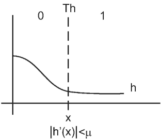
8.3.2 Dynamic background subtraction algorithm using DB (DBSDB)
In this section, we describe an on-line algorithm that handles video sequences that are captured by a static camera. We assume that the background is dynamic (moving). The DBSDB applies an off-line procedure that captures the dynamic background and an on-line background subtraction algorithm. In addition, the DBSDB algorithm segments the video sequence after the background subtraction is completed.
The input to the algorithm consists of two components:
-
•
Background training data: A video sequence of the scene without foreground objects. This training data can be obtained for instance from the frames in the beginning of the video sequence. This sequence is referred to as the background data (BGD).
-
•
Data for classification: A video sequence that contains background and foreground objects. The classification of the objects is performed on-line. We refer to this sequence as the real-time data (RTD).
For both input components, the video frames are assumed to be in RGB - see Fig. 8.3.
The algorithm is applied to every video frame and a binary mask is constructed in which the pixels that belong to the background are set to 0 while the foreground pixels are set to 1.

8.3.2.1 Iterative method for capturing a dynamic background - training
The algorithm that is described in Section 8.3.1.3, does not handle well on-going changes in the background, such as illumination differences between frames, moving leaves, water flowing, etc. In the following, we present a method that is not affected by background changes.
An iterative procedure is applied on the BGD in order to capture the movements in the scene. This procedure constitutes the training step of the algorithm. Let be the BGD input sequence and let be the output background frame. is initialized to zeros. Each iteration contains the following steps:
-
•
Application of the off-line algorithm (Section 8.3.1.1) in order to capture the static background of . The BGD is treated as a single sliding window of length . The output consists of the background frames and where is the normalization of .
-
•
is subtracted from each frame in by , . In case the input is in grayscale format, we set to zero each pixel in that has a negative value. The output is the sequence .
-
•
is added to by .
-
•
is the input for the next iteration, .
The iterative process stops when a given number of pixels in are equal to or smaller than zero. Finally, is normalized to be between 0 to 255. The normalized background is denoted by . The output of this process is composed of and .
8.3.2.2 The DBSDB algorithm
In this section, we describe the DBSDB algorithm which handles video sequences that contain a dynamic background. The DBSDB algorithm consists of five steps. The first and second steps are training steps which capture the background of the BGD by processing the RGB sequence and its corresponding gray-scale sequence, respectively. The third and fourth steps classify to foreground and background the RTD using the result of the first and second steps. The final step combines the output from the third and fourth steps.
Formally, let
and be the
RTD, which is the on-line captured video sequence, and the BGD, which
is the off-line video sequence for the training step (Section 8.3.2.1),
respectively.
The DBSDB algorithm consists of the following:
Step 1: The grayscale training
-
•
Convert into grayscale format. The grayscale sequence is denoted by .
- •
-
•
Capture the dynamic background (DBG) in (Section 8.3.2.1). The output is the background frame given by .
Step 2: The RGB training
Step 3: The grayscale classification
is converted into grayscale format. The grayscale sequence is denoted by . The SBSDB algorithm is applied to as it is described in Section 8.3.1.3, excluding the threshold computation (Section 8.3.1.4). The output is denoted by .
For each frame , , we do the following:
-
•
is subtracted from by . Then, each pixel in that has a negative value is set to 0.
-
•
A threshold is applied to . The threshold is computed as in Section 8.3.1.4. The output is set to:
for .
Step 4: The RGB classification
For each frame , , we do the following:
-
•
is subtracted from by .
-
•
is normalized to be between 0 to 255. The normalized frame is denoted by .
-
•
A threshold is applied to every channel in . The derivation of the threshold is described in Section 8.3.2.3. The output is set to:
for .
Step 5: The DFS step
This step combines the and from the grayscale and RGB classification steps, respectively. Since contains false negative detections (not all the foreground objects are found) and contains false positive detections (background pixels are classified as foreground pixels). Therefore, we use each foreground pixel in as a reference point from which we begin the application of a DFS on . This step is described in details in Section 8.3.2.4.
8.3.2.3 Threshold computation for RGB input
In the following, we describe how the threshold for the RGB classification step (step 4) is derived. The last step of the DBSDB algorithm derives thresholds that are applied in order to separate between background pixels and foreground pixels in each of the RGB components. The DBSDB algorithm subtracts the background from the input frame. Consequently, the histogram of a frame after the subtraction is high in the center and low at the right and left ends, where the center area corresponds to the background pixels. The DBSDB algorithm smooths the histogram in order to compute the threshold values accurately.
Let be the histogram and let be a given parameter which provides a threshold for the slope of . should be chosen to be the absolute value of the slope where becomes moderate. We denote the thresholds to be and . We scan from its global maximum to the left. if is the first coordinate that satisfies where denotes the first derivative of at point , i.e. the slope of at point . We also scan from its global maximum to the right. if is the first coordinate that satisfies .
The classification of the pixels in the input frame is determined according to and . For each color component and for each
See Fig.8.4 for an example how the thresholds are derived.
The process is executed three times, one for each of the RGB channels. The outputs are combined by a pixel-wise OR operation.
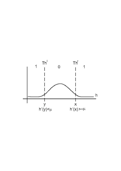
8.3.2.4 Scan by depth-first search (DFS)
The last step of the DBSDB algorithm is the application of a DFS. Let and be the output frames of the grayscale and the RGB classification steps (steps 3 and 4), respectively. Each frame is a binary mask represented by a matrix. The DFS step combines both outputs. In there are false negative detections and in there are false positive detections. We use each foreground pixel in as a reference point from which we begin a DFS in . The goal is to find the connected components of the graph whose vertices are constructed from the pixels in and whose edges are constructed according to the 8-neighborhood of each pixel.
The graph on which the DFS is applied, is constructed as follows:
-
•
A pixel is a root if is a foreground pixel and it has not been classified yet as a foreground pixel by the algorithm.
-
•
A pixel is a node if it is a foreground pixel and was not marked yet as a root.
-
•
Let be a node or a root and let be a matrix that represents its 8-neighborhood. A pixel is a child of if is a node (see Fig.8.5).
The DFS is applied from each root in the graph. Each node, that is scanned by the DFS, represents a pixel that belongs to the foreground objects that we wish to find. The scanned pixels are marked as the new foreground pixels and the others as the new background pixels.
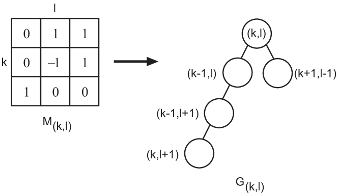
8.3.3 A parallel extension of the SBSDB and the DBSDB algorithms
We propose parallel extensions to the SBSDB and the DBSDB algorithms. We describe this scheme for the SBSDB algorithm. Nevertheless, the same scheme can be used for the DBSDB algorithm.
First, the data cube (Eq. 8.1) is decomposed into overlapping blocks . Next, the SBSDB algorithm is independently applied on each block. This step can run in parallel. The final result of the algorithm is constructed using the results from each block. Specifically, the result from each block is placed at its original location in . The result for pixels that lie in overlapping areas between adjacent blocks is obtained by applying a logical operation on the corresponding blocks results.
8.4 Experimental results
In this section, we present the results from the application of the SBSDB and DBSDB algorithms. The section is divided into three parts: The first part is composed from the results of the SBSDB algorithm when applied to a SBG video. The second part contains the results from the application of the DBSDB algorithm to a DBG video. In the third part we compare between the results obtained by our algorithm and those obtained by five other background-subtraction algorithms.
8.4.1 Performance analysis of the SBSDB algorithm
We apply the SBSDB algorithm to a video sequence that consists of 190 grayscale frames of size . The video sequence was captured by a static camera with a frame rate of 15 fps. The video sequence shows moving cars over a static background. We apply the sequential version of the algorithm where the size of the SW is set to 5. We also apply the parallel version of the algorithm where the video sequence is divided to four blocks in a formation. The overlapping size between two (either horizontally or vertically) adjacent blocks is set to 20 pixels and the size of the SW is set to 10. Let be the test frame and let be the SW starting at . In Fig. 8.6 we show the frames that contains. The output of the SBSDB algorithm for is shown in Fig. 8.7.
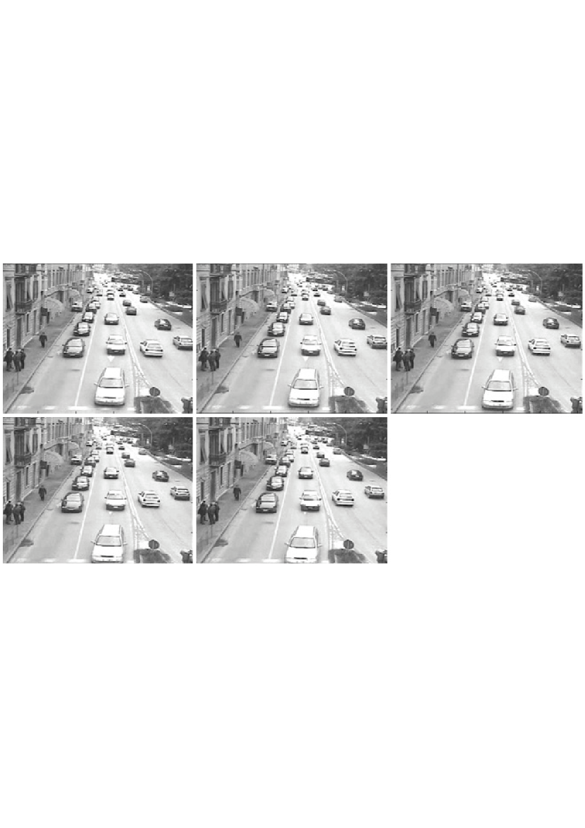
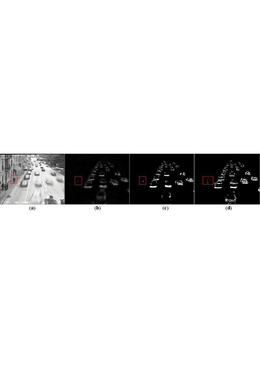
8.4.2 Performance analysis of the DBSDB algorithm
We apply the DBSDB algorithm to five RGB video sequences. The first four video sequences have a frame rate of 30 fps. The last video sequence has a frame rate of 24 fps. All the video sequences, except the first video sequence, are of size . The first video sequence is of size . The video sequences were produced by a static camera and contain dynamic backgrounds.
The input video sequences are:
-
1.
People walking in front of a fountain. It contains moving objects in the background such as water flowing, waving trees and a video screen whose content changes over time. The DBSDB input is a RTD that contains 170 frames and a BGD that contains 100 frames. The output of the DBSDB is presented in Fig. 8.8(g).
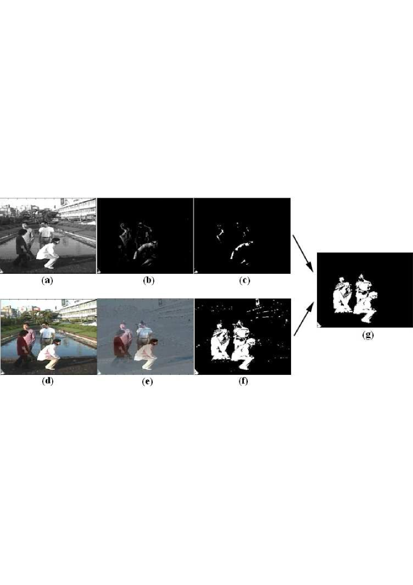
Figure 8.8: (a), (d) The original test frames in grayscale and RGB, respectively. (b), (e) The grayscale and RGB test frames after the background subtraction in the classification steps (steps 3 and 4) of the DBSDB algorithm, respectively. (c), (f) Results after the thresholding of (b) and (e), respectively. (g) The final output of the DBSDB algorithm after the application of the DFS. -
2.
A person walking in front of bushes with waving leaves. The DBSDB input is a RTD that contains 88 frames and a BGD that contains 160 frames. The output of the DBSDB algorithm is presented in Fig. 8.9(g).
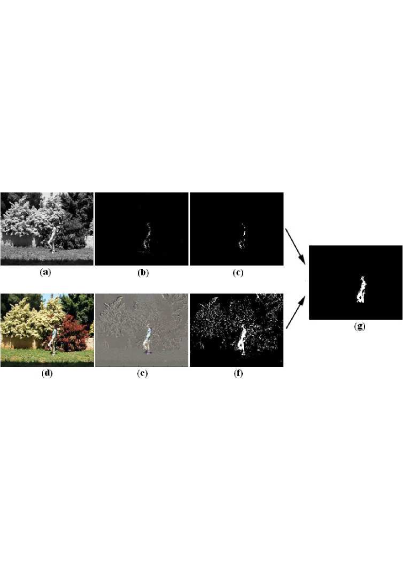
Figure 8.9: (a), (d) The original test frames in grayscale and RGB, respectively. (b), (e) The grayscale and RGB test frames after the background subtraction in the classification steps (steps 3 and 4) of the DBSDB algorithm, respectively. (c), (f) Results after the thresholding of (b) and (e), respectively. (g) The final output of the DBSDB algorithm after the application of the DFS. -
3.
A moving ball in front of waving trees. The DBSDB input is a RTD that contains 88 frames and a BGD that contains 160 frames. A frame from the video sequence is shown in Fig. 8.10(a). The output of the DBSDB algorithm is presented in Fig. 8.10. Figure 8.10(d) contains the result of the sequential version of the algorithm and Fig. 8.10(g) contains the results of the parallel version. In results of the parallel version, the video sequence was divided to four blocks in a formation. The overlapping size between two (either horizontally or vertically) adjacent blocks was set to 20 pixels and the size of SW was set to 30.
- 4.
-
5.
A person walking in front of a sprinkler. The DBSDB input is a RTD that contains 121 frames and a BGD that contains 100 frames. A frame from the video sequence is shown in Fig. 8.10(c). The output of the DBSDB algorithm is presented in Fig. 8.10(f).
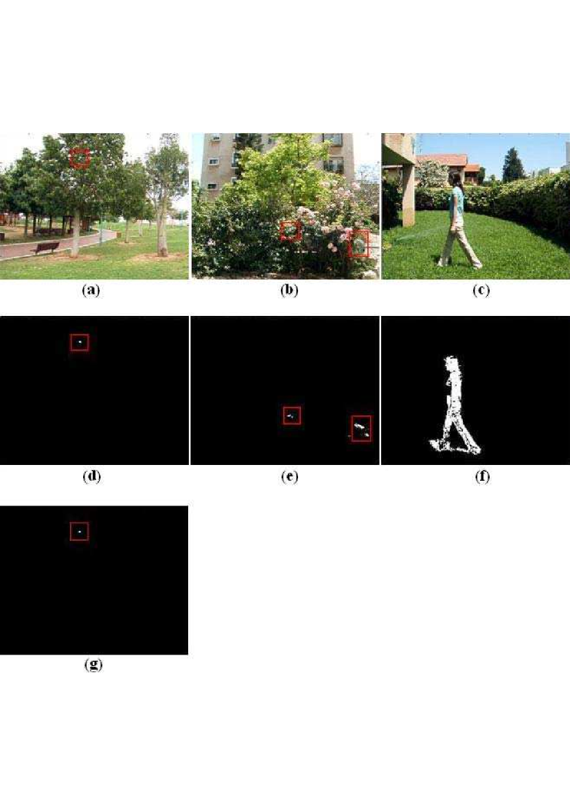
Figure 8.10: (a)-(c) The original test frames. (d)-(g) The segmented outputs from the application of the DBSDB algorithm. (a) A ball in front of waving trees. (d), (g) The result of the sequential and parallel versions of the algorithm applied on (a), respectively. (b), (e) A ball jumping in front of a tree and a car passing behind the trees. (c), (f) A person walking in front of a sprinkler.
8.4.3 Performance comparison between the BSDB algorithm and other algorithms
We compared between the BSDB algorithm and five different background subtraction algorithms. The input data and the results were taken from [215]. All the test sequences were captured by a camera that has three CCD arrays. The frames are of size 160x120 in RGB format and are sampled at 4Hz. The test frame that was segmented, in video sequences where the background changes, is taken to be the frame that appears 50 frames after the frame where the background changes. On every output frame (besides the output of the BSDB algorithm), a speckle removal [215] was applied to eliminate islands of 4-connected foreground pixels that contain less than 8 pixels. All other parameters were adjusted for each algorithm in order to obtain visually optimal results over the entire dataset. The parameters were used for all sequences. Each test sequence begins with at least 200 background frames that were used for training the algorithms, except for the bootstrap sequence. Objects such as cars, which might be considered foreground in some applications, were deliberately excluded from the sequences.
Each of the sequences poses a different problem in background maintenance. The chosen sequences and their corresponding problems are:
-
1.
Background object is moved - Problem: A background object that changes its position. These objects should not be considered as part of the foreground. The sequence contains a person that walks into a conference room, makes a telephone call, and leaves with the phone and a chair in a different position. The test frame is the one that appears 50 frames after the person has left the scene.
-
2.
Bootstrapping - Problem: A training period without foreground objects is not available. The sequence contains an overhead view of a cafeteria. There is constant motion and every frame contains people.
-
3.
Waving Trees - Problem: Backgrounds can contain moving objects. The sequence contains a person walking in front of a swaying tree.
-
4.
Camouflage - Problem: Pixels of foreground objects may be falsely recognized as background pixels. The sequence contains a monitor on a desk with rolling interference bars. A person walks into the scene and stands in front of the monitor.
We apply six background subtraction algorithms to the five video sequences, including the algorithm that is presented in this chapter. The background subtraction algorithms are:
-
1.
Adjacent Frame Difference - Each frame is subtracted from the previous frame in the sequence. Absolute differences greater than a threshold are marked as foreground.
-
2.
Mean and Threshold - Pixel-wise mean values are computed during a training phase, and pixels within a fixed threshold of the mean are considered background.
-
3.
Mean and Covariance - The mean and covariance of pixel values are updated continuously [121]. Foreground pixels are determined by applying a threshold to the Mahalanobis distance.
-
4.
Mixture of Gaussians - This algorithm is reviewed in Section 8.2.
-
5.
Eigen-background - This algorithm is reviewed in Section 8.2.
-
6.
BSDB - The algorithm presented in this chapter (Section 8.3).
The outputs of these algorithms are shown in Fig. 8.11.
We applied the SBSDB algorithm to the first two video sequences: the moved chair and the bootstrapping. In both cases, the background in the video sequence is static. In the first video sequence, the SBSDB algorithm handles the changes in the position of the chair that is a part of the background. The SBSDB algorithm does not require a training process so it can handle the second video sequence where there is no clear background for training. Algorithms that require a training process can not handle this case.
We applied the DBSDB algorithm to the waving trees and the camouflage video sequences. In both cases, the background in the video sequences is dynamic. In the moving trees video sequence, the DBSDB algorithm captures the movement of the waving trees and successfully eliminates it from the video sequence where as the other algorithms produce false positive detections. The DBSDB algorithm does not handle well the last video sequence where the foreground object covers the background moving object (the monitor). In this case the number of false negative detections is significant.

8.5 Conclusion and future work
We introduced in this chapter the BSDB algorithm for automatic segmentation of video sequences. The algorithm contains two versions: the SBSDB algorithm for video sequences with static background and the DBSDB algorithm for video sequences that contain dynamic background. The BSDB algorithm captures the background by reducing the dimensionality of the input via the DB algorithm. The SBSDB algorithm uses an on-line procedure while the DBSDB algorithm uses both an off-line training procedure and an on-line procedure. During the training phase, the DBSDB algorithm captures the dynamic background by iteratively applying the DB algorithm on the background training data.
The BSDB algorithm presents a high quality segmentation of the input video sequences. Moreover, it was shown that the BSDB algorithm produces results that are highly competitive with current state-of-the-art algorithms by coping with difficult situations of background maintenance.
The performance of the BSDB algorithm can be enhanced by improving the accuracy of the threshold values. Furthermore, it is necessary to develop a method for automatic computation of , which is used in the threshold computation (Sections 8.3.1.4 and 8.3.2.3).
Additionally, the output of the BSDB algorithm contains a fair amount of false negative detections when a foreground object obscures a brighter background object. This will be improved in future versions of the algorithm.
The BSDB algorithm can be useful to achieve low-bit rate video compression for transmission of rich multimedia content. The captured background is transmitted once followed by the detected segmented objects.
Chapter 9 Automatic Identification of Features in Hyper-Spectral Data
In this chapter we show how to uniquely construct a spectral signature that enables to identify and distinguish spectrally unique materials in a data base of spectral signatures.
This Chapter uses the basic concepts of hyper-spectral imagery which were introduced Chapter 5. This is followed by a detailed overview of the image-processing method that we introduce as well as two algorithms that implement this approach.
9.1 Introduction
In this chapter, we introduce a new approach that chooses only certain band values from the inspected substance. These values reflect the physical properties of the material. In this sense, we achieve dimensionality reduction, and make it easy to link between the resultant match and the material’s properties.
After extracting the “interesting” features two methods for the analysis of the signal are presented:
- 1. Exact search:
-
Building a tree structure classifier, using only a part of the extracted data (depends on the spectral library size).
- 2. Approximate search:
-
Constructing a classifier, which enables to find spectra that have some common features with the target.
The rest of this chapter is organized as follows: related works are presented in Section 9.2. Section 9.3 describes the algorithm for extraction of spectral features. In Section 9.4 we introduce the exact search, including: tree construction, target identification and illustration. The approximate search, including: the feature distribution table, the target identification and an example are described in Section 9.5.
9.2 Related work
Several algorithms for the analysis of hyper-spectral imagery can be found in the literature. Most of them suffer from the following disadvantage: physical properties of the materials under inspection are not used during the data processing. Consequently, when the output results are analyzed, it is hard to understand how the the material characteristics are connected to reasons that led to the results/identification. Another common disadvantage of existing methods is that they tend to use all the data in the hyper-spectral image (e.g. Spectral Angle Mapper [33]). We assume that a large portion of this data is unnecessary, and adds complexity. Moreover, in our proposed algorithm, the comparison between spectral signatures is based on the location of the spectral features in the spectrum. This means that the reflectance value of the spectral feature at this location does not affect the comparison.
In the following, we describe current state-of-the-art methods for spectral identification.
- Spectral Angle Mapper (SAM)
-
([126, 128, 127]). The reflectance of a hyper spectral pixel can be described as an -dimensional vector, where is the number of bands. The length of the vector is the brightness, and the direction of this vector can be regarded as the spectral features that are contained in the pixel. Changes in the illumination affect only the length of the vector but not its angle. The classification of a target is done by calculating the angle between the vector of the analyzed pixel and the vectors (representing materials) from the spectral libraries/database. The pixel that classifies the material is the one with the lowest spectral angel value.
The drawback of the SAM method is that it does not distinguish between positive and negative correlation values since it takes into account only the absolute value of the correlation. The SCM method was designed to overcomes this limitation.
- Spectral Correlation Mapper (SCM)
-
([33]). This method performs a similar computation to the one that is performed by the SAM method. Namely, the angles between the spectra DB and the analyzed pixel. However, the SCM method standardizes the vectors of the reflected spectra. Thus, the Pearsonian Correlation Coefficients (PCC) are used.
- Spectral Identification Method (SIM)
-
([31, 32]). This method uses the statistical procedure ANOVA ([57, 201, 204, 222]) that is based on linear regression. It is not affected by negative correlation values. By combining it with the SCM coefficients, it uses the negative/positive information. This technique exhibits three estimates according to the levels of significance of the materials.
- Spectral Feature Fitting (SFF)
-
([42]). This approach examines the specific absorption features in the spectra. The U.S. Geological Survey ([44]) has developed an advanced method based on this approach called Tetracorder. SFF is a simpler method that is based on this approach.In this technique, the user defines a range of wavelengths which form a unique absorption feature that exists in the chosen target (the isolation of the feature is done using a continuum mathematical function). Often the highpoint enclosing the feature is identified and a line fit between points is used in order to normalize the absorption feature by embedding the original spectra into the continuum. The comparison is based on the following two characteristics: The depth of the features in the target versus the depth in the analyzed pixel and the shape of the features in the target versus the shape in the analyzed pixel (using a least-square technique).
- Optimum Index Factor (OIF)
-
([38]). In this method, an index, which is called the OIF, is used to select the optimal combination of any number of bands in the satellite image in order to create a color composite. The bands that contain the highest amount of information are chosen. The OIF is based on the total variance within bands and correlation coefficients between bands. Every combination of bands is assigned an OIF. The optimal combination of bands, which is chosen, is defined as the combination of bands with the lowest correlation coefficient between bands and with the highest total variance within bands.
This approach is quite different from the previous approaches. While other approaches try to deal with the whole spectrum, this approach reduces the high-dimensionality of the data (manifested as superfluous data with high inter-band correlation).
The approach that is introduced in this chapter follows the logic of OIF (selection of specific band for classification) and deals with the high-dimensionality of the data, unlike all the methods that were introduced above.
9.3 Feature extraction
The spectra data that is used as input to the proposed algorithm represent absorption values. Nevertheless, it can operate in the same way if the spectra represent radiation, reflection or any other type of hyper-spectral data. The description of the general algorithm is accompanied by a detailed example of a database that contains 173 entries (spectra) each of which contains 2001 wavelengths. The length of each spectrum (vector) in the database is predefined - in our case it is 2001 - which is the number of wavelengths. In order to construct a robust and efficient classifier, the dimensionality of the vectors has to be reduced. This is achieved by extraction of characteristic features of the spectra. If a spectrum is treated as a continuous curve, then its geometrical characteristics are determined by the physical properties of the material. We use four types of geometrical characteristics to represent the physical properties that can facilitate the unique identification of a spectral signature of the material in the database. We demonstrate it on the following four features111A different number and type of physical features can be chosen.:
-
1.
Location of deep minima.
-
2.
Location of shallow and one-side minima.
-
3.
Location of near-horizontal flat intervals.
-
4.
Location of inflection points.
These features describe a spectral signature based upon the absorption features and back-scattering parameters of the material. Deep minima correspond to wavelengths where the light absorption is high while shallow and one-side minima correspond to wavelengths where the light absorption is small to moderate. Near-horizontal flat intervals correspond the subranges of the spectrum where the absorption amount is approximately constant. Finally, inflection points are locations in the spectrum where there is a change in the manner the light is absorbed. Specifically, looking at the spectrum subranges on both sides of the inflection point, the rate and direction of absorption will change from one subrange to the other. We demonstrate the strength of this spectral signature using the clay minerals Montmorillonite and Kaolinite. Both minerals have an absorption band at 2205 nm where as only Kaolinite has an additional small absorption band at 2165 nm (shallow minima). The proposed method enables to distinguish between these two clay minerals and points out their different features. Both the inflection point position of an absorption band and flat intervals in a spectral signature, are features that help to distinguish between spectral features. Currently, our experiments show that the order in which the selected features are chosen does not affect the final result. However, the order of the selected features might affect the final output when different parameters, which correspond to different physical assumptions, are chosen.
The four features that we use were chosen to demonstrate the performance of the proposed algorithm. Nevertheless, one can exclude some features or add new features. For example, the area below two adjacent minima can be another feature. There is no limitations on the number of features and their meaning. Any feature can be added, provided its effectiveness was established.
The problem is to correctly locate essential physical events even in the presence of strong noise. Let be a set of original raw spectra of length (number of wavelengths). We denote by
the first and the second centered differences of the array y, respectively. The resulting sets , and are assumed to be corrupted by noise. Therefore, we filter their elements by applying a low-pass shape-preserving B-spline filter. The smoothed arrays are denoted by , and .
9.3.1 Finding the locations of the features
In the following, we describe how the locations of the four features are found. Five thresholds are used during the calculation.
- Location of deep/shallow minima:
-
First, we find all the points , where the sequence changes its sign, i.e. where or . Without loss of generality, we describe the procedure for points where . We classify the deep/shallow minima points in the following way: let be a marked point and let be the point such that for all . Let be the point such that for all . We denote by and the intervals to the left and to the right of the point , respectively. We calculate , , and and apply the following conditions:
-
•
If then we discard the point .
-
•
If and then we mark the point as a deep minima.
-
•
If but then we mark the point as a shallow or one-side minima.
-
•
- Location of near-horizontal flat intervals:
-
We find intervals of length of a given length in which . The central points of these intervals, which we denote by , mark the locations of near-horizontal flat intervals.
- Location of inflection points:
-
First, we find all the points , where the second difference changes its sign i.e. and or and . Without loss of generality, we describe the inflection points classification procedure for points where and . We denote by the point such that for all and we denote by the point such that for all . Let and be the wide and narrow neighborhoods of the point , respectively. We calculate and . We discard the point if (near flat interval) or if (near vertical interval). The set of points that were not discarded are marked as inflection points.
Thinning the features arrays:
In order to make the feature extraction robust to noise, the feature vector is thinned in the following way:
-
•
If an interval of a given length , contains several deep minima points, we retain for that interval only the deepest minimum point i.e. the point for which the value of is the smallest. Other points inside the interval are discarded.
-
•
A similar procedure is applied to shallow minima points, indicators of flat intervals and inflection points. However, in the latter case, points with the smallest values are retained.
Merging the features arrays
After finding the feature points, they are merged into a single feature vector. The merging procedure considers the features in the following order: deep minima points, shallow minima points, flat intervals and inflection points. This order does not affect the output of the algorithm. It only affects the structure of the classifier tree. Consequently, we carry out the following procedures:
-
•
If within distance of ( is chosen empirically) samples from an inflection point lies a minimum point or an indicator of a flat interval then this inflection point is discarded.
-
•
If within distance of samples from an indicator of a of flat interval lies a minimum point then this indicator is discarded.
-
•
If within distance of samples from a shallow minimum lies a deep minimum point then this shallow minimum point is discarded.
Finally, for a given spectrum , we get a reduced set of features, which we arrange as a matrix where denotes a maximal number of sought after features per feature type.
Example: The construction is illustrated by a specific example in which .
| (9.1) |
The structure of the matrix in Eq. 9.1 is as follows: The first row contains the wavelengths of deep minima points. There are only three such points and thus the rest of the row is filled with zeros. The second row contains the wavelengths of shallow minima points. The third row contains the wavelengths of indicators of flat intervals and the last row contains the wavelengths of the first ten inflection points. We display the spectrum and its features in Figure 9.1.
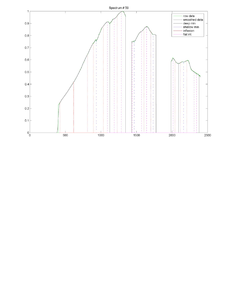
9.4 Exact search
In this section, we introduce an algorithm that looks for a material whose spectral signature matches exactly the spectral signature of a given material.
9.4.1 Construction of the classification tree
We design a tree structured classifier that, using characteristic features of a spectrum, assigns it to a certain material from the given database. Here is the outline of the construction of this classifier.
- Initialization:
-
As an input data, we use the extracted selected features for all the spectra in the database. The data is organized in four matrices , , of sizes . The rows correspond to different spectra. The columns of contain the wavelength locations of the extracted features from all the spectra. Specifically, the columns of contain the locations of deep minima points of all spectra in ascending order, the columns of contain the shallow minima points, the columns of contain indicators of flat intervals and the columns of contain the inflection points. We can visualize this as four matrices as is illustrated in Fig. 9.2.
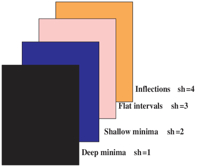
Figure 9.2: The arrangement of four matrices
We now construct the tree. The first node of the tree includes all the spectra in the database. The tree construction uses a rule to split each node to a son node and a daughter node. At each split, one feature (one of the deep minima, shallow minima etc.) is examined to see whether it distinguishes between the different spectra. The son node is assigned with all the spectra that cannot be distinguished by this feature while the daughter node is assigned with those that can. This procedure is repeated recursively for every node until each node contains a single spectrum or all the features have been exhausted.
- Split of the first node:
-
We start with the matrix , . We introduce a shift parameter and initialize its value to zero. The column in the matrix contains the locations of the first deep minimum of all the spectra. Let .
The first node in the tree is split according to the following Split rule: All the spectra, such that ( is a given tolerance parameter for distance comparison whose value is determined empirically) are assigned to the son node. The rest of the spectra (if it is not empty) is assigned to the daughter node. The split value is saved as as well as the parameters and .
- Handling of the daughter node:
-
If this node contains only one object then it is marked as a terminal node. Otherwise, the node is stored for subsequent processing. The shift parameter is left unchanged.
- Handling of the son node:
-
If this node contains only one object, then it is marked as a terminal node. Otherwise, the following steps are performed. Recall that the entries in in column number are all equal to the same value (up to samples). Therefore, if , then we continue to the next column by . If or if then we proceed to the next matrix by increasing by 1 and setting . This means that the deep minima features are not sufficient for separation of the objects which belong to the son node and we go to the next set of features. Then, the node is subjected to a split. However, if the son node is a terminal node, then the daughter node, which shares the same parent node with the son node, is subjected to a split.
- Split of the node number nod:
-
We take the matrix . Let . The Split rule is: All the spectra, such that , are assigned to the son node. The rest of the spectra (if not empty) is assigned to the daughter node. The split value is saved as as well as the parameters and .
- Handling of a daughter node:
-
As above.
- Handling of a son node:
-
As above. A possible situation that may happen for some son node, is when the parameters become and . This means that the objects within this node are identical with respect to the available set of features. In this case, the node is marked as a terminal node.
The above steps are repeated until all the nodes become terminal nodes. Then, the tree is saved and the terminal nodes that contain more than one material are saved separately.
We emphasize that the order in which the matrices are processed is unimportant. Using a different processing order will produce a different tree structure, however, the outcome of the identification will be the same. This is due to the fact that every pair of different spectra can be distinguished by a set of features. Going over this set in any order will always distinguish between the spectra once all the distinguishing features have been visited.
9.4.2 Identification of a spectrum
- Input:
-
A raw spectrum from the given database and the constructed tree.
- Extraction of features:
The identification procedure traverses the tree starting from the root.
- Traversal decision at the first node:
-
Initially, the object lies in node 1, whose split value is . In the root node we calculate the difference . If then the traversal continues to the son node, otherwise – it continues to the daughter node. If the destination node is a terminal then we already have the answer.
- Traversal decision at an arbitrary node nod:
-
Assume that the traversal arrived at a non-terminal node nod. Assume the parameters at this node are , and the split value is . We calculate the difference . If then the traversal continues to the son node, otherwise – it continues to the daughter node.
The traversal of the tree continues until the object reaches a terminal node. The output is an index of the identified spectrum and the features that were actually involved in its identification. If the spectrum belongs to a group of identical spectra in the database, then the output of the classifier consists of the indices of the whole group.
9.4.3 Illustration by example of the tree construction
In the following a step-by-step of the tree construction in Section 9.4.1 is illustrated using an example. From the given database (173 entries of spectra where each consists of 2001 wavelengths), we select the eight spectra which are given in Table 9.1. We let and .
| Serial number | 1 | 2 | 3 | 4 | 5 | 6 | 7 | 8 |
|---|---|---|---|---|---|---|---|---|
| Row number in the database | 173 | 4 | 27 | 87 | 43 | 163 | 150 | 156 |
Their corresponding graphs are given in Fig. 9.3.
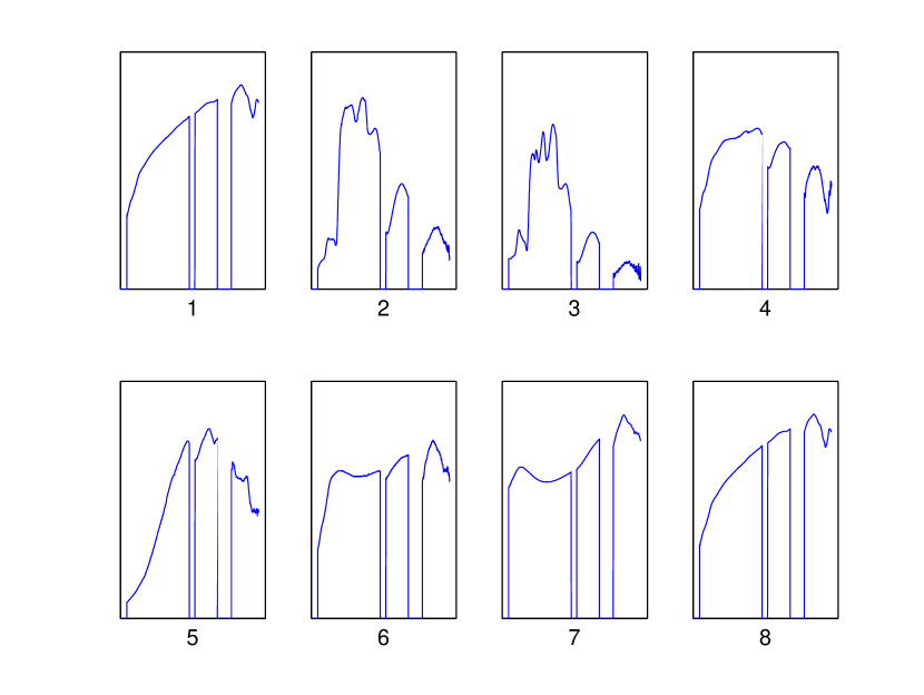
The first node of tree consists of the eight spectra. The matrix in Eq. 9.2 is the ten deep minima of each spectra. Column 1 is the serial number of the spectra in the database as specified in Table 9.1.
| (9.2) |
We look at the second column of matrix (Eq. 9.2). We look for the minimum value in this column and we get that it is . The distances from feature (deep-minima) locations 672, 673 from are less or equal to . Therefore, we assign rows 2 and 3 to the son node while the others are assigned to the daughter node (see Fig. 9.4).

The matrix for the son is set to:
| (9.3) |
The matrix for the daughter is set to:
| (9.4) |
We continue with the third column of (Eq. 9.3).
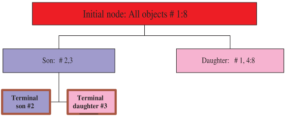
We get that the . Entry 3 in is a terminal son, and entry 2 in is a terminal daughter. The current structure of the tree is given in Fig. 9.5.
We now proceed to (Eq. 9.4). Calculating for the second column yields . Therefore, entry 4 is a son terminal node, and the rest is daughter node. The resulting structure of the tree is given in Fig. 9.6.
The matrix (Eq. 9.4) for the daughter becomes:
| (9.5) |
Calculating for the first column of produces . Therefore, the current node is split into a son terminal node, which contains material 5, and a daughter node which contains the rest. The tree structure that has been constructed so far is given in Fig. 9.7:
The matrix for the daughter (Eq. 9.5) is:
| (9.6) |
Te value of for the first column is . Therefore, the node is split into a son node which contains materials 1 and 8 and a daughter node which contains materials 6 and 7. The resulting structure of the tree is given in Fig. 9.8:
The matrices for son and daughter are:
| (9.7) |
and
| (9.8) |
We check the third column of the son in Eq. 9.7. Since it contains zero values, we go to matrix .
| (9.9) |
Both entries are assigned to son and we go to matrix .
| (9.10) |
The algorithm continues to check the columns in an attempt to separate between entries. Finally, it reaches matrix which is given by
| (9.11) |
Since we arrived at the last feature, this node appears to be unsplittable. Consequently, the node is marked as terminal and we continue to the remaining daughter. The current structure of the tree is given in Fig. 9.9:
We process the daughter in Eq. 9.8. Here it is again
| (9.12) |
The second column contains identical values. Therefore, both materials are assigned to a son node and we go to , which yields
| (9.13) |
The entries in the second column are identical up to the feature distance tolerance , therefore, they are both assigned to a son. Next, we check the third column. The distance between the entries is , therefore, entry 7 is a son terminal-node and entry 6 is a daughter terminal-node. However, because many features of these two spectra are similar, it is most probable that these spectra are associated with the same material. The final tree is given in Fig. 9.10:
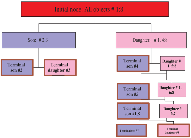
9.4.4 Experimental results
As mentioned above, the spectra database that we use contains the absorption values of materials with 2001 wavelengths. We have 173 vectors which are composed of 2001 wavelengths. There are seven pairs of identical spectra in the given database: [160 161], [154 172], [152 170], [111 165], [112 164], [153 171], [156 173].
The thresholds that we use are: , , , , . - length of flat interval, length of thinning interval, - merging threshold, - distance tolerance parameter for exact search comparisons (for the definition of all threshold parameters, the reader is referred to Section 9.3.1. The maximal number of sought after features per feature-type was set to .
We display a few outputs from the identification process. Figure 9.11 demonstrates the identification of material . The identification was achieved by merely using the two deep minima that are located at wavelengths and .
Figure 9.12 depicts the spectrum graph of material . Its signature consists of three deep minima and three shallow minima. The spectral signature of material is includes only one shallow minima as it is illustrated in Fig. 9.13. The spectra graphs of materials and are depicted in Fig. 9.14. This materials are identical and the identification process succeeded not to distinguish between them after using all their spectral features during the identification process.
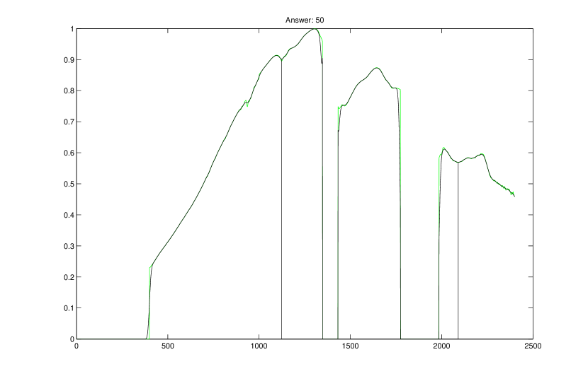
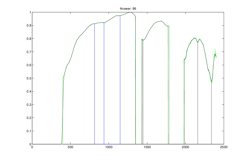
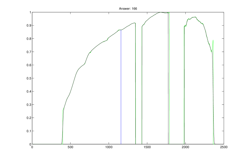
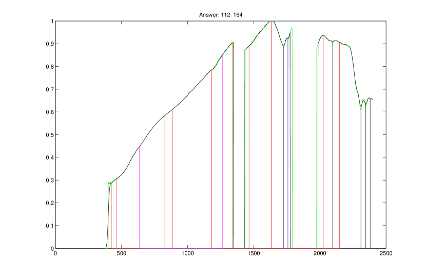
9.5 Approximate search
9.5.1 Introduction
In this section we describe a search scheme for a specific spectrum in a given database that produces spectra that are similar to the presented spectrum. We call this scheme approximate search. It uses the same characteristic features that were described in Section 9.4 - the exact search scheme. The new classifier is tailored to find all spectra in the database that have some common features with the presented spectrum (up to a predefined tolerance interval). There are no limitations on the number of spectra in the database that the classifier can handle. This classifier is especially useful when applied to noisy measurements. It can also be utilized to perform unmixing where the measurements of endmembers are corrupted with noise.
9.5.2 The approximate search scheme
The scheme consists of three operational blocks:
- 1.
-
Feature extraction block - produces a diverse set of geometric features from the spectra in the given reference database. These features are related to the physical properties of their corresponding materials.
- 2.
-
Feature distribution table construction block - provides a table that describes the distribution of the selected features among the spectra in the reference database. It provides a fast search for the spectra, which possess the prescribed features.
- 3.
-
Identification block - extracts selected features from the presented spectrum by using the feature distribution table (block 2). Then, it finds all the spectra in the given database that have some features close to the features of the presented spectrum. The closeness is measured using a given parameter which will be defined later. This block produces as output a set of spectra that are similar to the presented spectrum. The algorithm can handle spectra that do not necessarily belong to the reference database.
We demonstrate the capabilities and the performance of the algorithm using two databases: The first, which is denoted by DB1, is the same database that was used in Section 9.4. The second database, which is denoted by DB2, consists of 90 spectra whose structure is similar to the structure of spectra from DB1. To validate the performance of the approximate search algorithm, three types of experiments were conducted:
-
1.
The reference database is DB1 and the tested spectra were taken from DB1.
-
2.
The reference database is DB2 and the tested spectra were taken from DB2.
-
3.
The reference database is DB1 and the tested spectra were taken from DB2.
Selection of features (block 1) is done as in Section 9.3.
9.5.3 Construction of the feature distribution table (block 2)
In the following, we describe the construction of the table that describes the distribution of the selected characteristic features among the spectra in the reference database.
- Organization of the input data:
-
As an input data, we use the extracted characteristic features of all spectra in the reference database (see Section 9.4). The data is organized in a matrix of size , . The rows correspond to different spectra () in the reference database. The initial columns in S contain the locations of deep minima points in ascending order of all spectra. If, for example, spectrum has only deep minima points, then, the positions are filled with zeros. Recall that the locations of all the features do not exceed 2500 in DB1 and DB2. This number corresponds to the highest wavelength at which the spectra was captured. We make use of this number to distinguish between different features in . The following columns are assigned to locations of shallow minima and are organized similarly to the previous columns. To distinguish between the shallow minima and deep minima, each sample is increased by adding . Column till contain indicators of flat intervals that are increased by adding , and the last columns, i.e. columns till , contain the locations of inflection points that are increased by adding 9000.
In the all the coming figures, the axis starts at 400. This number corresponds to the minimal wavelength at which the spectra were captured.
Figure 9.15 displays the spectra from DB1. Tables 9.2-9.5 show the wavelength locations of the deep minima, shallow minima, flat interval indicators and inflection points, respectively. In these tables, was taken to be .
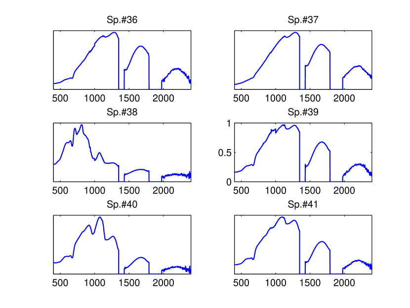
Figure 9.15: Spectra from DB1. 36 669 1157 0 0 0 0 0 0 0 0 37 1162 1446 0 0 0 0 0 0 0 0 38 673 743 1008 1185 2011 2236 2337 0 0 0 39 670 1009 1171 1444 0 0 0 0 0 0 40 432 672 973 1167 2001 2148 2343 0 0 0 41 671 1168 1445 0 0 0 0 0 0 0 Table 9.2: Deep minima locations in ascending order of spectra are placed in the initial columns of the matrix S. 36 4454 5008 5143 5166 5196 5299 5322 3000 3000 3000 37 5155 3000 3000 3000 3000 3000 3000 3000 3000 3000 38 3616 5046 5067 5088 5117 5188 3000 3000 3000 3000 39 3970 4119 5008 5043 5171 5197 5232 5261 5290 3000 40 3619 5039 5062 5088 5117 5181 5215 5260 3000 3000 41 3420 3617 5056 5169 5258 5324 3000 3000 3000 3000 Table 9.3: Shallow minima locations added by 3000 in ascending order of spectra are placed in columns 11-20 of the matrix S. 36 6458 6598 6931 7121 7283 7669 8084 6000 6000 6000 37 6470 6592 6658 7131 7286 7449 7665 6000 6000 6000 38 6420 7224 7455 7556 7646 6000 6000 6000 6000 6000 39 6453 6600 7274 7451 7673 6000 6000 6000 6000 6000 40 6645 6916 7077 7265 7450 6000 6000 6000 6000 6000 41 6454 6644 6932 7094 7269 7453 7673 7996 8087 6000 Table 9.4: Flat intervals locations added by 6000 in ascending order of spectra are placed in columns 21-30 of the matrix S. 36 9424 10238 9000 9000 9000 9000 9000 9000 9000 9000 37 9425 9929 11049 11094 9000 9000 9000 9000 9000 9000 38 9861 9000 9000 9000 9000 9000 9000 9000 9000 9000 39 9428 9841 10063 10022 9000 9000 9000 9000 9000 9000 40 9472 9832 9000 9000 9000 9000 9000 9000 9000 9000 41 9843 9000 9000 9000 9000 9000 9000 9000 9000 9000 Table 9.5: Inflection points locations added by 9000 in ascending order of spectra are placed in columns 31-40 of the matrix S. - Initialization of the feature distribution table T:
-
In the beginning, the size of T is unknown. The largest size of T is where is the total number of different features found in the entire database. Let be a binary row vector of zeros, where is the number of spectra in the reference database. The column in the matrix S contains the locations of the first deep minimum of all the spectra. Let . We set .
Selection Criterion: We find for all the spectra in the reference database such that where the parameter determines the tolerance interval.
Let the indices of these spectra that satisfy the Selection Criterion be . We set , . Locations that contain 1 mark indices of the spectra that satisfy the Selection Criterion i.e. indices of spectra that have a deep minimum whose distance from is not greater than . We define the first row of table T to be .
- First update of the feature matrix :
-
We update the matrix S in the following way. For each , rows correspond to the indices marked in the previous step. All these rows are subjected to one-sample left side shift. Formally,
(9.14) It may happen that after the shift by Eq. 9.14, the first columns in some row become . It means that spectrum has only one deep minima which is within distance from . In this case, we apply additional shifts of the type in Eq. 9.14 to row until a non-zero term appears at the column 1. These rows are discarded since all their deep minima were considered. These spectra are reconsidered when other feature types are being processed e.g. shallow minima. Note that terms that are equal to 3000, 6000 or 9000 are also treated as 0. Thus, a set of features in spectrum other than deep minima (most probably, shallow minima) appear at the first ten positions. These features will be considered no sooner than when all the deep minima features of all the spectra in the reference database are used. The output is the updated feature matrix .
- Complement of table T:
-
We repeat the above operations on the updated feature matrix . Thus, we produce the second row in table T and the updated feature matrix . Subsequent iterations produce more rows in table T that correspond to the ascending sequence of features. The values of the features appear at the first column of table T. During the updating process of the feature matrix , some rows become 0 (or 3000,6000, 9000). We remove these rows from the matrix . Thus, its size is reduced. The iterations continue until the matrix becomes a one-row matrix consisting of zeros (or 3000,6000, 9000).
Table is completed. Its first column comprises all the features present in the matrix in ascending order. This number of features is . The remaining columns consist of zeros and ones. Locations of ones indicate spectra that have a feature. For example, if and then it means that spectrum has a feature at the location 1520 (up to a tolerance interval ). Since , this feature is a deep minimum. If and then it means that spectrum has a feature at location 4715-3000=1715 (up to a tolerance interval ). Since , this feature is a shallow minimum.
| Features | 36 | 37 | 38 | 39 | 40 | 41 |
|---|---|---|---|---|---|---|
| 973 | 0 | 0 | 0 | 0 | 1 | 0 |
| 1008 | 0 | 0 | 1 | 1 | 0 | 0 |
| 1157 | 1 | 1 | 0 | 0 | 1 | 0 |
| 1168 | 0 | 0 | 0 | 1 | 0 | 1 |
| 1185 | 0 | 0 | 1 | 0 | 0 | 0 |
| 1444 | 0 | 1 | 0 | 1 | 0 | 1 |
| 2001 | 0 | 0 | 1 | 0 | 1 | 0 |
From table 9.6 we see that spectra and have a deep minimum at location 1008, spectra and have a deep minimum at location 1444, etc.
| Features | 36 | 37 | 38 | 39 | 40 | 41 |
|---|---|---|---|---|---|---|
| 3616 | 0 | 0 | 1 | 0 | 1 | 1 |
| 3970 | 0 | 0 | 0 | 1 | 0 | 0 |
| 4119 | 0 | 0 | 0 | 1 | 0 | 0 |
| 5008 | 1 | 0 | 0 | 1 | 0 | 0 |
| 5039 | 0 | 0 | 1 | 1 | 1 | 0 |
| 5056 | 0 | 0 | 0 | 1 | 0 | 0 |
| 4623 | 0 | 0 | 0 | 0 | 1 | 1 |
From table 9.7 we see that spectra and have shallow minimum at location 616=3616-3000, spectra and have shallow minimum at location 2008=5008-3000, etc.
| Features | 36 | 37 | 38 | 39 | 40 | 41 |
|---|---|---|---|---|---|---|
| 6453 | 1 | 0 | 0 | 1 | 0 | 1 |
| 6592 | 1 | 1 | 0 | 1 | 0 | 0 |
| 6644 | 0 | 0 | 0 | 0 | 1 | 1 |
| 6931 | 1 | 0 | 1 | 0 | 0 | 1 |
| 7121 | 1 | 1 | 0 | 0 | 0 | 0 |
| 7265 | 0 | 0 | 0 | 1 | 1 | 1 |
| 7283 | 1 | 1 | 0 | 0 | 0 | 0 |
From table 9.8 we see that spectra and have flat interval at location 453=6453-6000, spectra and have flat interval at location 1121=7121-6000, etc.
| Features | 36 | 37 | 38 | 39 | 40 | 41 |
|---|---|---|---|---|---|---|
| 9424 | 1 | 1 | 0 | 1 | 0 | 0 |
| 9472 | 0 | 0 | 0 | 0 | 1 | 0 |
| 9832 | 0 | 0 | 0 | 1 | 1 | 0 |
| 9861 | 0 | 0 | 1 | 0 | 0 | 0 |
We see from table 9.9 that spectra and have an inflection point at location 424=9424-9000, spectra and have an inflection point at location 832= 9832-9000, etc.
9.5.4 Identification of a spectrum
- Input:
-
A raw test spectrum and the constructed feature distribution table T (as was described in Section 9.5.3) are loaded. The test spectrum may or may not belong to the reference database.
- Extraction of features:
-
The features of spectrum are extracted according to the procedure described in Section 9.3. The features are gathered into the row vector , whose structure is similar to the structure of a row in the matrix S with the difference that we discard the values 0, 3000, 6000 and 9000. For example,
(9.15) is the features of spectrum 39 without 0, 3000, 6000 and 9000 (see tables 9.2, 9.3, 9.4 and 9.5).
- Reduction of the feature distribution table T:
-
Recall that for , the first column of in table T contains all the features from the reference database. Also, is the number of spectra in the reference database and is the number of features. We define an indicator column vector which is initialized with zeros. Next, we test all the features in the following way: if the feature is close to a feature , , such that
(9.16) then, we set , where is a tolerance parameter. It may happen that inequality 9.16 is valid for two features and . In this case, we choose . Let be the set of indices such that .
Finally, we prepare , which is the reduced version of table T that contains only rows whose indices belong to i.e.
Table 9.10 presents a portion of the reduced feature distribution table for the spectra , which corresponds to deep minima (see table 9.2).
S.36 S.37 S.38 S.39 S.40 S.41 669 1 0 1 1 1 1 1008 0 0 1 1 0 0 1168 0 0 0 1 0 1 1444 0 1 0 1 0 1 1 1 2 4 1 3 Table 9.10: Portion of the reduced feature distribution table for the spectra . - Finding spectra that have common features with the presented spectrum:
-
For this purpose, we calculate for the sums of the columns of the reduced table that correspond to the spectra in the reference database:
The value of determines the number of features in spectrum from the database that coincide (up to the tolerance parameter ) with the features of the presented spectrum . The values of for Table 9.10 are given in its bottom row.
Note that the user can use all the available sets of features (deep and shallow minima, flat intervals an inflection points) or any combination of these sets. In the above example (table 9.10), only deep minima are considered.
- Histograms:
-
We elaborate the above process using histograms of the total number of spectra that have common features against the number of common features. In other words, we calculate the numbers of common features .
The histogram in Fig. 9.16 displays the distribution of spectra from the reference database (spectra to ) according to the number of common features (deep minima) with the presented spectrum (). We can see that three spectra have only one common feature with spectrum , where as one spectrum has two common features and one spectrum has three common features with spectrum .
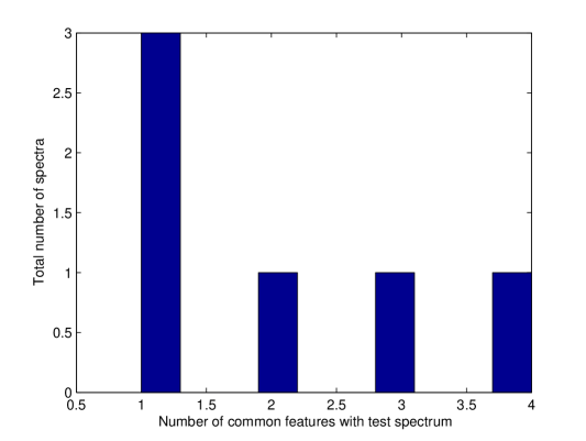
Figure 9.16: Distribution of spectra to from DB1 according to the number of common features (deep minima) with the presented spectrum from DB1. The histogram in Fig. 9.17 displays the distribution of spectra from the full reference database (spectra to ) according to the number of common features (deep minima) with the presented spectrum .
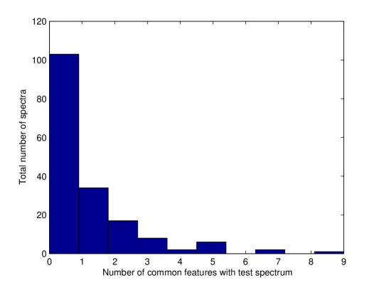
Figure 9.17: Distribution of spectra to from DB1 according to the number of common features (deep minima) with the presented spectrum from DB1. Two spectra have seven (deep minima) features with spectrum , six spectra have five common deep minima with spectrum .
The histogram in Fig. 9.18 displays the distribution of spectra from the full reference database (spectra to ) according to the number of common features (from all the available sets of features) with the presented spectrum .

Figure 9.18: Distribution of spectra to from DB1 according to the number of common features (from all available features) with the presented spectrum from DB1. - The output from the identification process:
-
Once the histogram related to the presented spectrum is displayed, the user indicates the number of common features to be used. Then, the algorithm produces a list of spectra that have (parameter) common features (up to the size of the tolerance parameter) with the presented spectrum.
9.5.5 Examples
This section included the results of the proposed feature extraction algorithm applied to spectra from DB1. For comparison, hierarchical clustering was applied on the investigated spectra using the shortest Euclidean distance measure for similarity. The Euclidean distance compares the entire spectrum regardless of the features.
9.5.5.1 Examples where both reference and test spectra are taken from DB1
In this section, the reference database is DB1 and the tested spectra belong to DB1 as well.
- Illustrations for the reduced database:
-
We searched the reduced database (spectra to ) for spectra that have common deep minima with spectra . We found that spectra has two and three common deep minima with spectrum and , respectively.
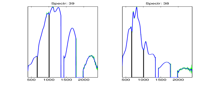
Figure 9.19: Spectrum from DB1 has two common deep minima with the tested spectrum , which is also in DB1. 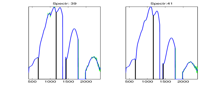
Figure 9.20: Spectrum from DB1 has three common deep minima with the tested spectrum , which also in DB1. We see from Fig. 9.19 that the materials that correspond to spectra and are weakly connected one to the other. A material that is more closely related to spectrum is spectrum , as can be seen from Fig. 9.20 where it is clearly demonstrated that spectra and originate from the same material. The hierarchical clustering algorithm found spectra and to have a weak similarity. However, it also found that spectrum is the closest to and not .
- Illustrations for the full database (deep minima):
-
We looked for similar spectra in DB1 (spectra to ). We define two spectra to be similar if most of their features are similar. We found that spectra and have seven common features (deep minima) with spectrum as it is illustrated in Figs. 9.21 and 9.22. It is clear that spectra and belong to the same material as spectrum . We also searched DB1 for materials the strongly resemble spectrum . Our results showed that spectra , , , , and have five common features with the tested spectrum . These findings are illustrated in Figs. 9.23-9.28.
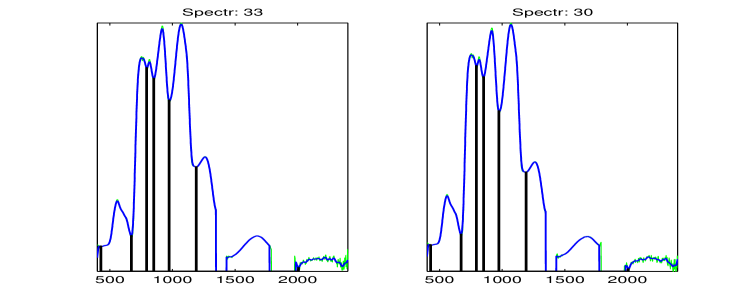

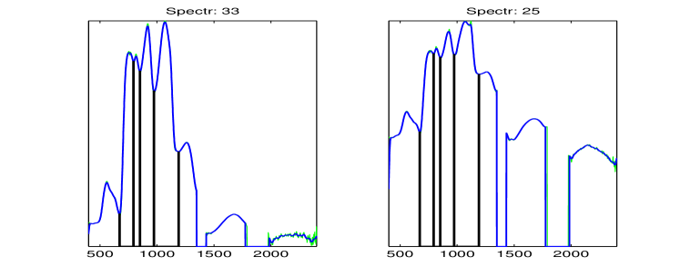
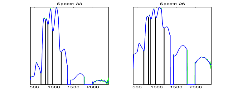
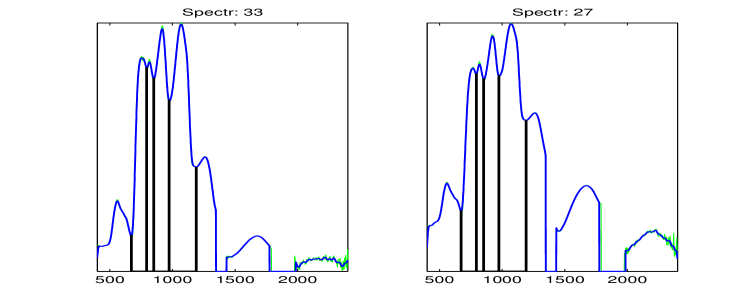
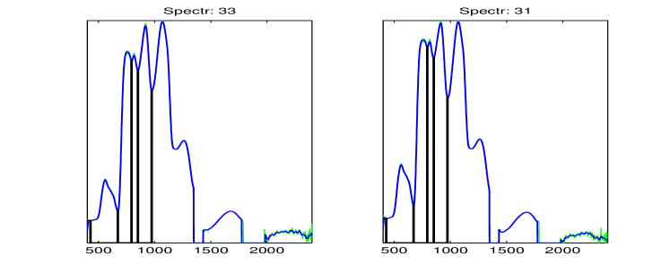
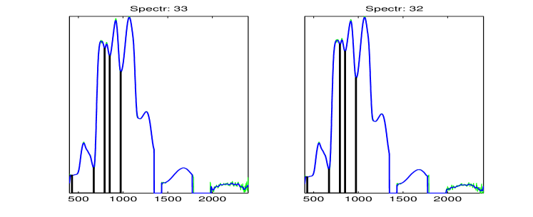
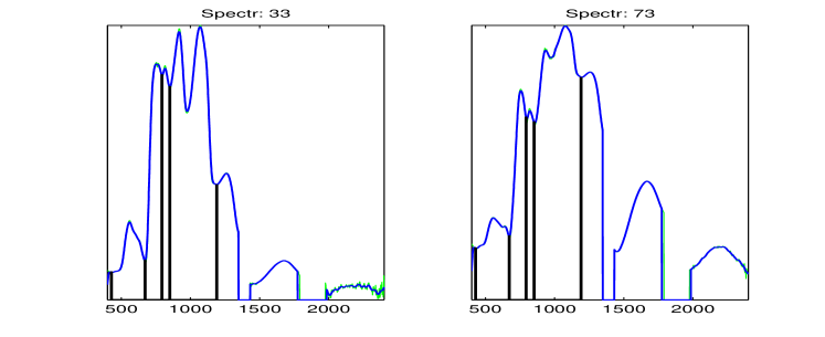
Obviously, spectra and are identical to spectrum . Moreover, it can be said that spectra , , , and originate from a similar material as spectrum . Most probably, this is also true for spectrum .
- Illustrations for the full database (inflection points):
-
We searched DB1 (spectra to ) for spectra that have common inflection points with spectrum . The histogram in Fig. 9.29 displays the distribution of spectra from DB1 according to the number of common inflection points with the tested spectrum .
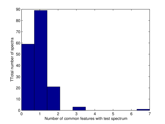
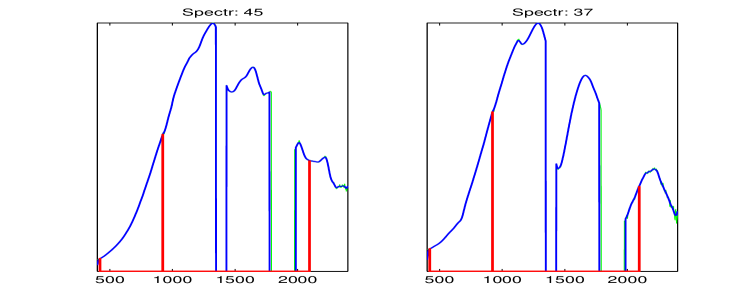
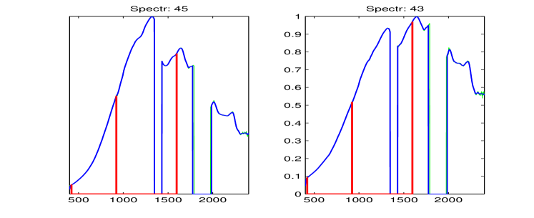
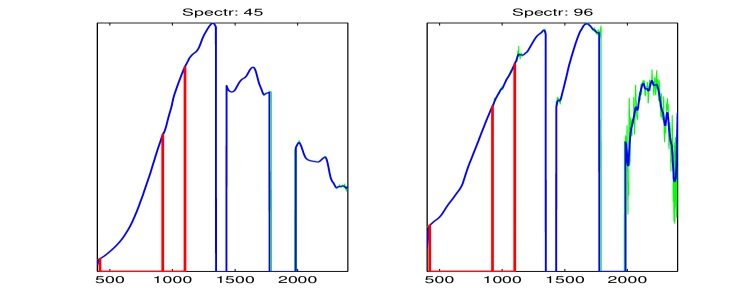
We can see from Figs. 9.30–9.32 that, most probably, spectrum is derived from the same material as , however, spectra and are very weakly related to spectrum . In general, common deep minima features indicate a closer relation between materials than inflection points do.
The hierarchical clustering algorithm failed to produce the deep-minima driven results of the proposed algorithm. Namely, spectra , and were put in different clusters. Moreover, spectra , , , and were also put in different clusters. Specifically, the clusters that include the above spectra were: [30] (singleton), [28 31], [21 32 33], [23 34], [25], [26], [27], [73]. The hierarchical clustering succeeded in finding the weak inflection point correlations. However it failed in finding the connection between spectra and . Spectra , , and were put in the following clusters: [35 37 42 43], [45 47 49] and [91 96 97 98].
9.5.5.2 Examples from DB2
In this section, the reference database is DB2 and the tested spectra also belong to the same reference database. Spectra from this database were smoothed. Typically, they have less characteristic features than spectra from DB1. Therefore, the identification process of these spectra uses all four sets of features (deep and shallow minima, flat intervals and inflection points).
We looked for materials in DB2 that have common features with spectrum from the same database (DB2). The histogram in Fig. 9.33 displays the distribution of spectra from the reference database DB2 (spectra to ) according to the number of all common features with the tested spectrum .

The identification algorithm found that six spectra – , , , , and – have at least three common features with spectrum . Two of them – and – have four common features with spectrum .
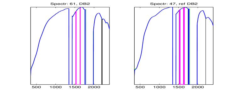
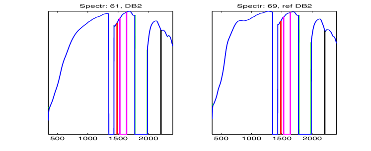
Our findings suggest that, spectra and are related to the same material that spectrum represents.
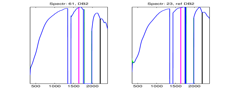
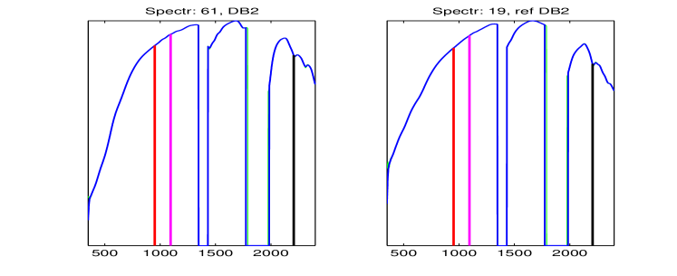
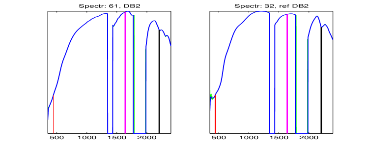

Figures 9.36-9.39 suggest that most probably, spectra , , and are related to materials whose physical properties are similar to the physical properties of the material that corresponds to spectrum .
The hierarchical clustering put spectrum in the same cluster as (their cluster also included spectra , and However, spectrum was put in a different cluster than ’s. Specifically, spectrum was put in a singleton cluster. Furthermore, spectra , , and were put in different clusters than ’s. Specifically, they were put in the following clusters: [56] (singleton), [18 19 59], [32 52], [6 22 23 26 53 68 72].
9.5.6 Example from different databases
In this section, the reference database is DB1 and the tested spectrum belongs to DB2. All four types of features (deep and shallow minima, flat intervals and inflection points) were used for the identification of the tested spectra.
First we looked for spectra from DB1 that are similar to spectrum from DB2. The histogram in Fig. 9.40 displays the distribution of spectra from the reference database DB1 (spectra to ) according to the number of common features with the tested spectrum from DB2.
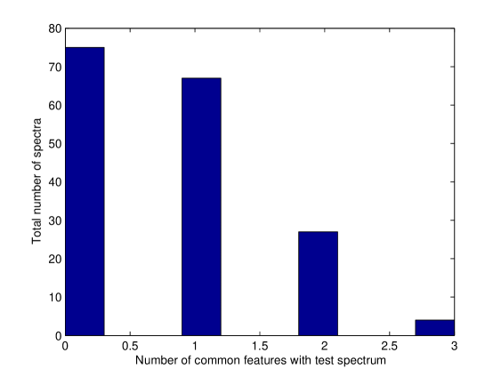
We found that four spectra , , and have three common features with spectrum .
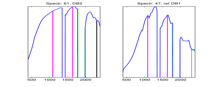

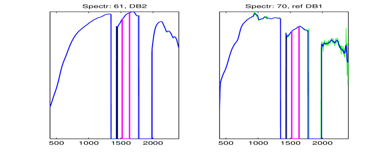
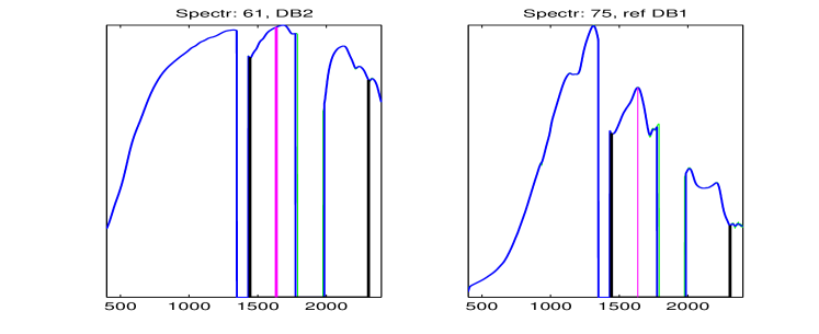
Although the spectra graphs look different, the findings show that the materials associated with spectra , , and from DB1 share some common physical properties with spectrum from . The hierarchical clustering algorithm clustered spectrum from DB2 only with spectrum from DB1.
9.6 Conclusion and discussion
In this chapter, dimensionality reduction was utilized to uniquely characterize substances via their spectral signatures. Specifically, characterizing features are extracted from the spectrum. Two complementary methods were presented for the computation and analysis of spectral signatures.
- Exact search:
-
A given spectrum is compared to all the spectra in a spectra database and only exact matches are sought after. Seven pairs of identical spectra were found. In most cases, only a small number of the available four feature types are utilized. Thus, we argue that the designed scheme is generic and can be applied to other databases. The algorithm allows different spectra in a population of spectra to have different resolutions (sampling rates).
- Approximate search:
-
The algorithm, which was described in this chapter, efficiently reveals the spectra in the reference database that posses similar physical properties as a spectrum tested for identification. The extent of the relation is interactively defined by the user. If the tested spectrum belongs to the reference database, then the algorithm correctly identifies it and finds all the spectra originating from the same material as well as the spectra that belong to a similar group of materials.
Other physical features can be chosen to either replace or enhance the current features that were described in this thesis such as the area between two minima, etc. Therefore, the algorithms can be classified as generic classifiers.
The results of the proposed algorithm were compared to those obtained by hierarchical clustering. It was found that in most cases hierarchical clustering fails to find connections between materials unless they are very similar. This renders hierarchical clustering to be suitable for exact search but not for inexact search.
Chapter 10 Wavelet-Based Acoustic Detection of Moving Vehicles
We propose a robust algorithm to detect the arrival of a vehicle of arbitrary type in the presence of various noise types. This is achieved by analysis of the acoustic signatures of vehicles and their comparison with an existing database of recorded and processed acoustic signals. We combine a construction of a training database of acoustic signatures of signals emitted by vehicles using the distribution of the energies among blocks of wavelet packet coefficients with a procedure of random search for a near-optimal footprint (RSNOFP). This construction achieves a minimum number of false alarms even under severe conditions such as the presence of signals emitted by acoustic sources that differ from those that appear in the training database. Such sources include helicopters, airplanes, wind, speech, footsteps etc. The proposed algorithm is robust even when the surrounding conditions of the test sites are completely different from the conditions where the training signals were recorded. The proposed technique has many algorithmic variations. For example, it can be used to classify different types of vehicles. The proposed algorithm is a generic solution for process control that is based on a learning phase (training) followed by an automatic real time detection. This is an example where dimensionality reduction is utilized for classification.
10.1 Introduction
The goal of the algorithm in this chapter is to detect the arrival of vehicles of arbitrary types such as various cars, vans, jeeps and trucks via the analysis of their acoustic signatures with a minimal number of false alarms. The algorithm uses an existing database of recorded acoustics signals. The problem is complex due to the high variability in vehicles types and the diversity of the surrounding conditions that may contain sounds emitted by planes, helicopters, speech, wind, steps, to name a few. These sounds also appear in many recordings in the training database. In addition, the velocities of the vehicles, their distances from the receiver, the roads where the vehicles traveled on are highly diverse as well. Consequently, this affected the recorded acoustics.
A successful detection depends on the constructed acoustic signatures that were built from characteristic features. These signatures enable to discriminate between vehicle (V) and non-vehicle (N) classes. Acoustic signals emitted by vehicles have a quasi-periodic structure. It stems from the fact that each part of the vehicle emits a distinct acoustic signal which contains only a few dominating bands in the frequency domain. As the vehicle moves, the conditions change and the configuration of these bands may vary, however, the general disposition remains. Therefore, we assume that the acoustic signature for the class of signals emitted by a certain vehicle is obtained as a combination of the inherent energies in blocks of wavelet packet coefficients of the signals, each of which is related to a certain frequency band. This assumption has been corroborated in the detection and identification of a certain type of vehicles ([9, 10]). The experiments in this section demonstrate that a choice of distinctive characteristic features that discriminate between vehicles and non-vehicle classes can be derived from blocks of wavelet packet coefficients. Extraction of characteristic features (parameters) is a critical task in the training phase of the process.
In order to identify the acoustic signatures, we combine in the final phase of the process the outputs of two classifiers. One is the well known Classification and Regression Trees (CART) classifier [26]. The other classifier is based on the distances between the test signal and sets of pattern signals from the V and N classes.
The chapter has the following structure: In Section 10.2, we briefly review related works. The structure of the available data is described in Section 10.3. In Section 10.4, we outline the scheme of the algorithm and in Section 10.7 we describe it in full details. Section 10.6 is devoted to presentation of the experimental results. Section 10.7 provides some discussion. Appendix I outlines the notions of the wavelet and wavelet packets and Appendix II provides a detailed description of the RSNOFP method.
10.2 Related work
Several papers that handle the separation between vehicle and non-vehicle sounds can be found in the literature. Choe et al. [39], extracted the acoustic features by using a discrete wavelet transform. The feature vectors were compared to the reference vectors in the database using statistical pattern matching to determine the type of vehicle from which the signal originated. In [73], discrete cosine transform was applied to signals and a time-varying auto-regressive modeling approach was used for their analysis. Averbuch et al. [9], designed a system that is based on wavelet packets coefficients in order to discriminate between different types of vehicles. Classification and Regression Trees (CARTs) were used for classification of new unknown signals. In a later paper [10], Averbuch et al. used similar methods with multiscale local cosine transform applied to the frequency domain of the acoustic signal. The classifier that was used was based on the Parallel Coordinates methodology [107]. Wu et al. [233] used the eigenfaces method [199], which was originally used for human face recognition, to distinguish between different vehicle sound signatures. The data was sliced into frames - short series of time slices. Each frame was then transformed into the frequency domain. Classification was done by projecting new frames on principal components that were calculated for a known training set. Munich [156] compared between several speech recognition techniques for classification of vehicle types. These methods were applied to short time Fourier transform of the vehicles’ acoustic signatures.
10.3 The structure of the acoustics signals
The recordings that we use in this section were taken under very different conditions on different time points. The recordings sampling rate (SR) was 48000 samples per second (SPS). It was downsampled to SR of 1000 SPS.
We extracted from the set of recordings, which were used for training the algorithm, fragments that contain sounds emitted by vehicles and stored them as the V-class signals. Recorded fragments that did not contain vehicles sounds were stored as the N-class signals. Both classes were highly diverse. Recordings in the V-class were taken from different types of vehicles during different field experiments under various surrounding conditions. In particular, the velocities of the vehicles and their distances from the recording device were different from one recording to the other. Moreover, the vehicles traveled on either various paved (asphalt) or unpaved roads, or on a mixture of paved and unpaved roads. Recordings in the N-class comprised of sounds emitted by planes, helicopters, wind gusts and speech nearby the receiver, to name a few.
Figure 10.1 displays portions of acoustic signals emitted by two cars with their Fourier transforms (spectra).
Figure 10.2 displays portions of acoustic signals emitted by a truck and a van with their Fourier transforms.
We see that the spectra of different cars differ from one another. It is even more apparent in the spectra of other vehicles. Figure 10.3 displays portions of acoustic signals emitted by a plane and a helicopter with their Fourier transforms, whereas Fig. 10.4 does the same for speech and wind patterns.
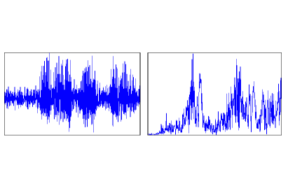
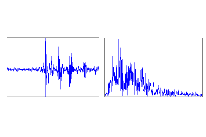
Analysis of the signals revealed that even within the same class (V or N), the signals differ significantly from one another. The same is true for their corresponding Fourier transforms. However, there are some properties that are common to the acoustic signals of all moving vehicles. First, these signals are quasi-periodic in the sense that there exist some dominating frequencies in each signal. These frequencies may vary as motion conditions change. However, for the same vehicle, these variations are limited to narrow frequency bands. Moreover, the relative locations of the frequency bands are stable (invariant) to some extent for signals that belong to the same vehicle.
Therefore, we conjectured that the distribution of the energy (or some energy-like parameters) of acoustics signals that belong to some class over different areas in the frequency domain, may provide a reliable characteristic signature for this class.
10.4 Formulation of the approach
Wavelet packet analysis (see Appendix I) is a highly relevant tool for adaptive search for significant frequency bands in a signal or a class of signals. Once implemented, a wavelet packet transform of a signal, although computationally efficient, yields a huge (redundant) variety of different partitions of the frequency domain. Due to the lack of time invariance in the multiscale wavelet packet decomposition, we use all the coefficients in the blocks of wavelet packet rather than individual coefficients and waveforms. The collection of energies in blocks of wavelet-packet-coefficients can be regarded as an averaged version of the Fourier spectrum of the signal. However, wavelet packets provide a more sparse and more robust representation of signals compared to the Fourier spectrum. We can see it, for example, in Fig. 10.5, where the displayed energies in their blocks of wavelet packet coefficients of the orthogonal spline wavelet of the sixth order in the sixth level of the wavelet packet transform of a car acoustic signal.
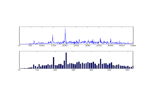
The algorithms in [9, 10] use a variation of the Best Basis algorithm [48, 228]. Specifically, it searches for a few blocks that best discriminate a certain vehicle from other vehicles and from the background. This approach did not prove to be robust and efficient for solving the problem of this chapter. This is due to the variability in vehicle types sought for in Class V and the different types of background in Class N. Therefore, another way to utilize the wavelet packet coefficients blocks was chosen. This method can be characterized as a random search for the near-optimal footprint (RSNOFP) of a class of signals. The proposed method utilizes ideas from compressed sensing [67, 64, 30].
In order to enhance the robustness of the algorithm, we implement three different versions of RSNOFP to corroborate one another.
The sample signals for the training phase and the on-line signals in the detection phase are formed by applying a short-time window on each input signal followed by a shift of this window along the signal so that adjacent windows are overlapped.
10.4.1 Outline of the approach
The proposed scheme consists of three steps:
- Training step:
-
We use a set of signals with known V/N classification. These signals are sliced into overlapped fragments of length (typically, ). The fragments are chosen according to the wavelet packet transform. The energies of the blocks are calculated and three versions of RSNOFP are applied. As a result, we represent each fragment by three different vectors of length (typically, or ). The components of these vectors constitute the characteristic features of the fragments. These vectors are used as pattern datasets and are also utilized to produce three versions of CART trees.
- Identification – features extraction step:
-
We slice the new acquired signal to overlapped fragments of length . Then, the wavelet packet transform is applied to each fragment. This is followed by calculation of the energies of the coefficient blocks. Then, we apply three different transforms that are determined according to the three versions of RSNOFP. As a result, we represent each fragment by three different vectors of length .
- Identification – decision making phase:
-
The three CART classifiers that were constructed in the training step are applied to the vectors that were produced by the previous step. In addition, the vectors are tested by a second classifier that calculates the distances of the vectors from the pattern datasets associated with the V and N classes. The final classification to V and N of the fragment is derived by combining the answers for the three vectors from the two classifiers.
10.5 Description of the algorithm and its implementation
10.5.1 The algorithm
The algorithm is composed of three basic phases:
- I.
-
Extraction of characteristic features from the V and N classes. It contains the following steps:
-
1.
The analyzing wavelet filters are chosen.
-
2.
The training sets of the signals are constructed by slicing the training signals into overlapped segments.
-
3.
The wavelet packet transform is applied to these segments.
-
4.
The energies in the blocks of the wavelet packet coefficients are calculated.
-
5.
The RSNOFP algorithm is executed. This embeds the training sets of signals into lower-dimensional reference sets that contain their characteristic features.
-
1.
- II.
-
Building the CART classification trees.
- III.
-
Classification of the new signal to either the V or the N class:
-
1.
The new signal is sliced into overlapped segments.
-
2.
The wavelet packet transform is applied to these segments.
-
3.
The energies in the blocks of the wavelet packet coefficients are calculated.
-
4.
The set of blocks energies of each segment is embedded into a lower-dimensional vectors that contains its characteristic features.
-
5.
The distances of the vector, which contains characteristic features, from the reference sets of V and N classes are calculated.
-
6.
The vector is tested by the CART classifier.
-
7.
The vector is classified to either the V or the N class.
-
1.
Next, we present a detailed description of the implementation of this algorithm.
10.5.2 Implementation
- Choice of the analyzing waveforms:
-
A broad variety of orthogonal and bi-orthogonal filters, which generate wavelet packets coefficients, are available ([55, 148, 12, 11]). We use the 6-th order spline wavelet. This filter reduces the overlap between frequency bands associated with different decomposition blocks. At the same time, the transform with this filter provides a variety of waveforms that have a fair time-domain localization. For details see Appendix I (Section 10.8).
- Signal preparation for training the algorithm:
-
Initially, we gather as many recordings as possible for the V and the N classes, which have to be separated. Then, we prepare from each selected recording, which belongs to a certain class, a number of overlapped slices – each of length samples, shifted by samples with respect to one another. In total, we prepare and slices for the V and N classes, respectively. The slices are arranged into two matrices, and .
- Embedding the sets of slices into sets of energies:
-
We use the normalized norms of the blocks as the energy measure. Then, the following operations are carried out:
-
1.
The wavelet packet transform up to scale (typically if ) is applied to each slice of length from the V and N classes. We take the coefficients from the sparsest (coarsest) scale . This scale contains coefficients that are arranged into blocks of length , each of which is associated with a certain frequency band. These bands form a near-uniform partition of size of the Nyquist frequency domain.
-
2.
The “energy” of each block is calculated using the chosen measure. We obtain, to some extent, the distribution of the “energies” of the -th slice 111We explain this for the class, however, this also applies to the class. In the later case, the corresponding notation is . over various frequency bands of widths , where is the Nyquist frequency. It is stored in the energy vector of length (typically, ). The energy vectors are arranged into two matrices, and . The -th row of the matrix is the vector . This vector is considered to be the averaged Fourier spectrum of the slice , as it is seen in Fig. 10.5. We consider this vector to be a proxy of the slice. By the above operations we reduced the dimension of the database by a factor of .
-
1.
- Embedding of sets of energies into the sets of features:
-
The subsequent operations yield a further reduction of the dimensionality in the compressed sensing [67, 64] spirit. It is achieved by the application of three versions of the RSNOFP scheme to the energy matrices and . The RSNOFP scheme is described in Appendix II. As a result, we get three pairs of the reference matrices: , and and the corresponding random matrices , and . These random matrices will be utilized in the identification phase.
- Compaction of the feature matrices in the V-class:
-
In order to refine the feature matrices of V-class, we test their rows. Recall that each row is associated with a segment of a signal that belongs to V-class. We calculate the Mahalanobis distances and of each row in the matrix from the sets and , respectively. We remove row from the matrix rows for which . The same is done for the matrices and .
- Conclusion:
-
As a result of the above operations, the dimensionality of the training set was substantially reduced. Typically, a segment of length 1024 is embedded into a 12-component vector. This part of the process might look computationally expensive, especially if, for better robustness, large training sets are involved. However, this procedure is called once and it is done off-line before the detection phase that is done on-line.
Figure 10.6 displays one row from matrix and one row from matrix . These are feature vectors that correspond to segments from the V-class and the N-class.
10.5.3 Building the Classification and Regression Trees (CARTs)
Once we have , and , which are three pairs of the reference matrices, we proceed to build the classifiers. For this purpose we use the vectors, which form rows in the reference matrices. The construction of the tree is done by a binary split of the space of input patterns so that, if a vector appears in the subspace , its classification can be predicted with sufficient reliability.
Given a test vector, the output of a CART classifier is the class to which the vector belongs and the probability of this classification. The basic idea behind the split is that the data in each descendant subset is more pure than the data in the parent subset. The scheme is described in full details in the monograph [26]. A brief outline of this method that is tailored to acoustic processing is given in [9].
After the construction of the three classification trees , and and the three pairs of reference matrices, we are in a position to classify new signals that were not used in the training phase.
10.5.4 Identification of an acoustic signal
An acoustic signal to be identified is preprocessed by the same operations that were used on the training signals.
- Preprocessing of a new acoustics signal:
-
Preprocessing is done similarly to the feature extraction phase (Section 10.5.2).
-
1.
The signal is sliced to overlapped segments of length samples each, shifted with respect to each other by samples. The wavelet packet transform up to scale is applied to each slice. We take the coefficients from the sparsest (coarsest) scale that are arranged into blocks of length . The “energy” of each block is calculated with the chosen measure. Thus, each -th slice is embedded into an energy vector of length . The energy vectors are arranged in the matrix where the -th row of the matrix is the vector.
-
2.
In order to embed the energy matrix into the feature spaces, we multiply it by the random matrices , and . These multiplications produce three feature matrices , and , where the -th row in each matrix is associated with the -th segment of the processed signal.
-
1.
- Identification of a single segment:
-
To identify the -th segment of a signal , we take three vectors , and , which form the -th rows of the matrices , and , respectively.
-
1.
These vectors are submitted to their respective versions , and of the classification tree. Once a vector is submitted to the tree, it is assigned to one of the subsets of the input space . These trees produce three decisions , and together with the corresponding probabilities , and . The decision determines the most probable membership of the segment. Here stands for rand, or pca or perm. The value if the CART assigns the segment to V-class and otherwise.
-
2.
The distances (for example, Mahalanobis or Euclidean) between the vectors , and and the respective pairs of the reference sets , and are calculated. This calculation produces three decisions , and together with the corresponding probabilities , and in the following way. Let and be the distances of a vector from the respective pair of the reference sets and . If then the decision is (the segment is assigned to V-class), otherwise (the segment is assigned to N-class). If then the membership probability in the V-class is defined as , otherwise . This classification scheme is similar to the well known Linear Discriminant Analysis (LDA) classifier [77]. If the Mahalanobis distance is used then it is identical to LDA. We call this scheme the Minimal Distance (MinDist) classifier.
-
3.
Two threshold values and are set and the results for the -th segment are combined into three 3-component column vectors , and , where:
(10.1)
- Identification of a recording:
-
1.
The vectors , and are gathered into three matrices , and of size , where is the number of overlapping segments produced from the analyzed signal. The vectors serve as the -th columns in the respective matrices .
-
2.
The rows of the matrices are processed by a moving average.
-
3.
The matrices , and are combined into the matrix in the following way. Each entry in is defined as the median value of the respective entries of the three matrices:
(10.2)
Conclusions:
The matrix contains the results for the analyzed signal. Its first row contains the averaged answers (which have significant probabilities) from the CART classifier. The value at each point is the number of positive (class V) answers in the vicinity of this point, which is divided by the length of the vicinity. It represents the “density" of the positive answers around the corresponding segment. The structure of the second row is similar to the structure of the first row with the difference that these answers come from the MinDist classifier instead of the CART classifier. The third row of the matrix combines the answers from both classifiers. First, these answers are multiplied. The combined answer is equal to one for segments where both classifiers produce the answer one (V-class) and zero otherwise. Thus, the classifiers cross-validate one another. Then, the results are processed by the application of the moving average providing the “density" for the positive answers. The third row in the matrix yields the most robust result from the detection process with minimal false alarm. For a binary detection scheme, any detection probability above 0.5 is considered as a detection.
The above scheme is described for the detection of the arrival of any moving vehicle. Obviously, the scheme is also applicable for the detection of the arrival of the sought after vehicles.
10.6 Experimental results
We conducted a series of experiments to detect the arrival of vehicles of arbitrary type in the presence of various types of noise.
Two hundred recordings were available. They were taken in five different areas. Many recordings contained sounds emitted by different vehicles combined with the sounds of wind, speech, aircrafts etc. The original sampling rate (SR) was 48000 samples per second (SPS). The signals were downsampled to SR of 1000 SPS. The motion dynamics, the distances of vehicles from the receiver and the surrounding conditions were highly diverse.
10.6.1 Detection experiments
The first task was to form the reference database of signals with known classification (training) for the construction of the classifiers. This database was derived from the recordings by clipping the corresponding fragments. The CAR fragments were extracted from 10 recordings whereas 5 recordings were used for the TRUCK fragments and the for the VAN fragments. Diverse non-vehicle fragments were extracted from 35 recordings. Thirty eight recordings, in total, were involved in the training process (most of them contained sounds from different sources). We tested various families of wavelet packets, various norms for the feature extraction and various combinations of features for the MinDist and CART classifiers. The best results were achieved with the wavelet packet transform that uses the sixth order spline filters and the norm.
We separated the reference signal s into two groups. One group (V class) contains all signal s associated with vehicles and the other group (N class) contains all the non-vehicles signals. The signals were sliced into overlapped segments of length that were shifted with respect to one another by , thus, the overlap was 3/4 of a fragment. We extracted the characteristic features from the segments as explained in Section 10.5.2. Each segment was expanded by the wavelet packet transform up to 6th level (scale) and the norm was used as an “energy" measure for all the 64 blocks of the 6th level. As a result of the procedures that were described in Section 10.5.2, we selected various sets of discriminant blocks. These procedures produced three pairs of reference matrices: , and with the corresponding random matrices , and . Each matrix has 12 columns according to the number of characteristic features. These matrices were used for the MinDist classification and were also utilized for building three CART trees , and . For the MinDist classification, we used all the available features (12), unlike building the CART trees, where better results were achieved with sets containing only 8 features.
All the available recordings were used in the detection phase. A recording number was embedded into the three feature matrices , and to associate the -th row of each matrix with the -th segment of the recording (see Section 10.5.4). Each row was tested with the MinDist and CART classifiers. The results were gathered into the matrix. The Euclidean distance was used for the MinDist classification.
In Figs. 10.7–10.15, we present a few results from the experiments on detection of vehicles of arbitrary types. All the figures have the same structure. Each is composed of four parts. The top part depicts the original recording . The three parts below the original recording present five rows from the matrix with respect to the time scale. The second part from the top presents the combined answers (the median from three answers) from the CART classifiers after being processed by the moving average. The third part from the top displays, in a similar manner, the results from the MinDist classifiers. The bottom figure illustrates the combined results from both classifiers i.e. the product of the answers from both classifiers after it was processed by the moving average. Any detection probability above 0.5 is considered as a detection.
10.6.1.1 Examples
- Recording :
-
We display in Fig. 10.7 the results for test recording . This recording was part of the training set. It is apparent that the arrivals of a car and a track at around the and seconds of the recording, respectively, are correctly detected by the CART and the MinDist classifiers.
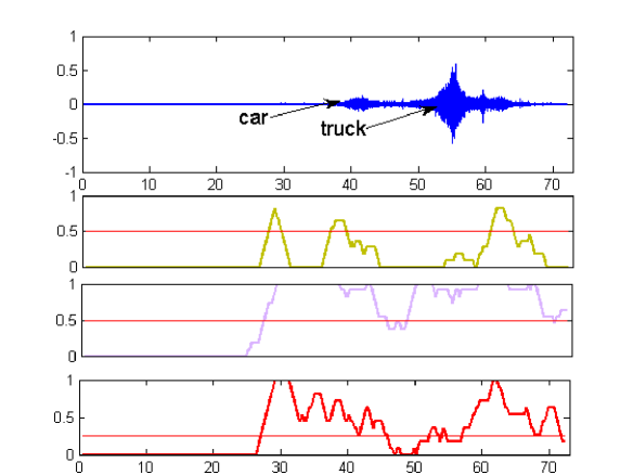
Figure 10.7: Results for test recording . The recording contains sounds emitted by a car (at around the second) and a truck (at around second). This recording was part of the training set. - Recording :
-
We display in Fig. 10.8 the results for test recording . This recording was part of the training set. Arrivals of two cars: one at the second and another at the second of the recording, respectively, are correctly detected by the CART and the MinDist classifiers. The sound of a helicopter became audible starting from the second of the recording until the end of the recording. It caused some false alarms, which were eliminated by combining the results of the classifiers (bottom figure).

Figure 10.8: Results for test recording . The recording contains sounds emitted by a car (at the second) and by another car (at the second). This recording was part of the training set. - Recording :
-
We display in Fig. 10.9 the results for test recording . A fragment of 60 seconds from the beginning of the recording was part of the training set of the N class. A loud speech is present in the background until vehicles pass by. It lasted during the first 100 seconds of the recording. In addition, there was a plane sound from the second until the end of the recording. A van briefly passed by at the second of the recording. It was correctly detected by the CART and the MinDist classifiers. The number of false alarms was reduced by combining the results of the classifiers (bottom figure).
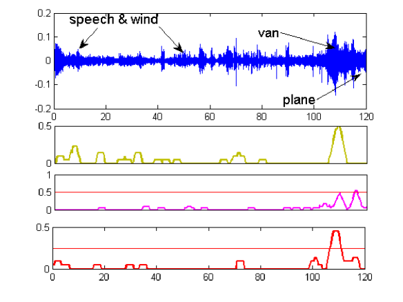
Figure 10.9: Results for test recording . The recording contains loud speech during the first 100 seconds, sounds emitted by a car (at around the second) and sound of a plane (from the second until the end of the recording). The fragment of the first 60 seconds of the recording was part of the training set of the N class. - Recording :
-
We display in Fig. 10.10 the results for test recording . This recording was not part of the training set. In the beginning of the recording, sound from a remote vehicle is heard. Then, a jumping vehicle passed by the receiver at around the , and seconds of the recording. In its last occurrence, it was followed by another car. All the events were correctly detected by the CART and the MinDist classifiers. The MinDist classifier produced some false alarms, which were eliminated by combining the results of the classifiers (bottom figure).

Figure 10.10: Results for test recording . In the beginning, the sound from a remote vehicle is heard. A jumping vehicle passed by the receiver at around the , and seconds of the recording. In its last occurrence, it was followed by another car. The recording was not part of the training set. - Recording :
-
We display in Fig. 10.11 the results for test recording . This recording was not part of the training set. In the beginning of the recording, a truck passed by the receiver followed by a pickup truck. A car followed by a truck passed by the receiver at around the second of the recording. A minibus and a car passed by the receiver at the end of the recording. All the events were correctly detected by CART and the MinDist classifiers. The MinDist classifier produced some false alarms, which were reduced by combining the results of the classifiers (bottom figure).
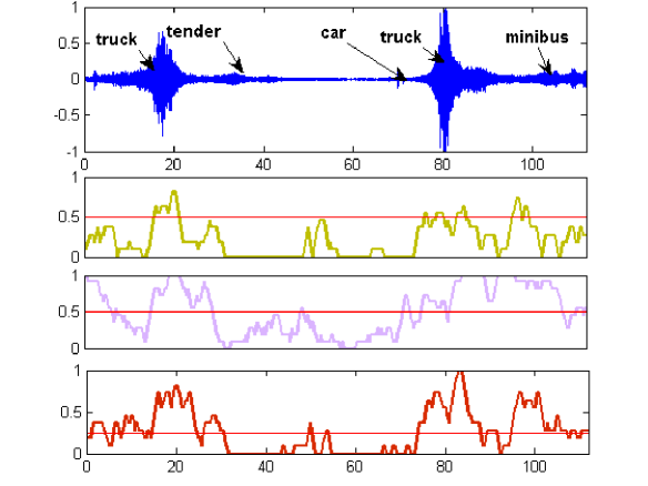
Figure 10.11: Results for test recording . In the beginning of the recording, a truck passed by the receiver followed by a pickup truck. A car followed by a truck passed by the receiver at around the second of the recording. A minibus and a car passed by the receiver at the end of the recording. This recording was not part of the training set. - Recording :
-
We display in Fig. 10.12 the results for test recording . The recording was not part of the training set. Two trucks passed by the receiver in opposing directions at around the second of the recording. Strong wind was present. The trucks were correctly detected by the CART and the MinDist classifiers. The MinDist classifier produced some false alarms, which were reduced by combining the results of the classifiers (bottom figure).
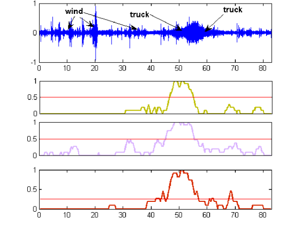
Figure 10.12: Results for test recording . Two trucks passed by the receiver in opposite directions at around the second of the recording. Strong wind was present at the site. The recording was not part of the training set. - Recording :
-
We display in Figs. 10.13 the results for test recording . The recording was not part of the training set. A truck passed by the receiver from the second to the second of the recording. Then, a strong sound of an airplane dominated the recording until the end of the recording. Strong wind sound appeared throughout the recording. The truck was correctly detected by the CART and the MinDist classifiers. The MinDist classifier produced some false alarms, which were reduced by combining the results of the classifiers (bottom figure). The plane was correctly not assigned to the V class.
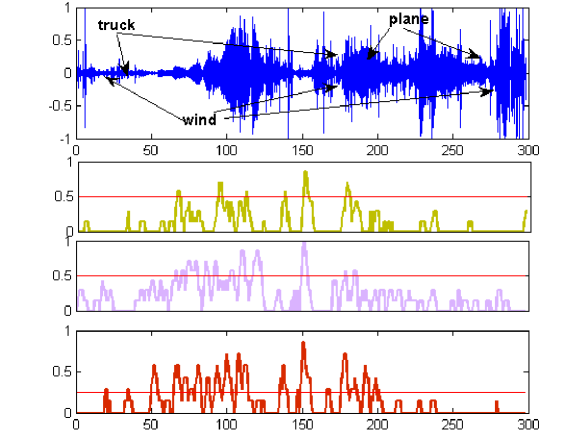
Figure 10.13: Results for test recording . A truck passed by the receiver from the second to the second of the recording. Then, a strong sound of an airplane dominated the recording until the end of the recording. Strong wind sound appeared throughout the recording. This recording was not part of the training set. - Recording :
-
We display in Figs. 10.14 the results for test recording . The recording was not part of the training phase. A truck followed by a minibus passed by the receiver at around the second of the recording. Another truck passed by at around the second. Strong wind was present. The vehicles were correctly detected by the CART and the MinDist classifiers. The MinDist classifier produced some false alarms, which were eliminated by combining the results of the classifiers (bottom figure).
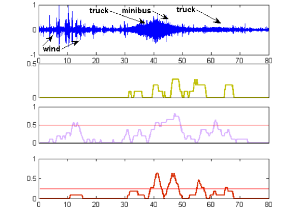
Figure 10.14: Results for test recording . A truck followed by a minibus passed by the receiver at around the second of the recording. Another truck passed by at around the second. Strong wind was present. This recording was not part of the training set. - Recording :
-
We display in Fig. 10.15 the results for test recording . The recording was not part of the training set. A sound of a truck was heard between the and the seconds and also between the and the seconds of the recording. An airplane sound appeared next. It lasted until the end of the recording. The truck was correctly detected by the CART and the MinDist classifiers. The plane was correctly not assigned to the V class. The MinDist classifier performed poorly.
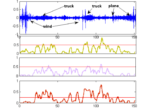
Figure 10.15: Results for test recording . A sound of a truck was heard between the and the seconds and also between the and the seconds of the recording. An airplane sound appeared next. It lasted until the end of the recording. This recording was not part of the training phase.
Comments
-
•
The detection experiments demonstrate the relevance of our approach to feature extraction.
-
•
A combination of three schemes for feature extraction performs better than any single scheme.
-
•
Combining the MinDist and the CART classifiers significantly reduces the number of false alarms.
-
•
The algorithm produced satisfactory detection results even when the conditions of the real signals essentially differ from the training data and the surrounding conditions. When the conditions of the captured signals are close to the training conditions, the detection is almost perfect.
-
•
The algorithm performs similarly on signal with sampling rates of 1000 SPS and 600 SPS. In a few cases, the results for SR of 1000 SPS were significantly better than those for SR of 600 SPS.
10.7 Conclusions and discussion
We presented a robust algorithm that detects the arrival of a vehicle of arbitrary type via the analysis of its acoustic signature using an existing database of recorded and processed acoustic signals for comparison.
To minimize the number of false alarms, we constructed an acoustic signature of a certain vehicle using the distribution of the energies among blocks which consist of its wavelet packet coefficients. This distribution serves as an averaged version of the Fourier spectrum of the signal. To reduce the dimensionality of the features sets, we designed a scheme of random search for the near-optimal footprint (RSNOFP), which proved to be an efficient tool for the extraction of a small number of characteristic features of the objects to be detected.
The following building blocks were used for the detection: (a) a classifier that is based on the minimal distance (MinDist) from the reference datasets and (b) the Classification and Regression Tree (CART) classifier. These classifiers cross-validated one another. The detection process is fast and can be implemented in real time.
This technology, which has many algorithmic variations, is generic and can be used to solve a wide range of classification and detection problems, which are based on acoustic processing such as process control, and, more generally, for classification and detection of signals which have near-periodic structure. Distinguishing between different vehicles can also be achieved via this technology.
The successful results were obtained using a low sampling rate. Therefore, the proposed method works well using very simple low-budget equipment.
10.8 Appendix I: The wavelet and wavelet packet transforms
Wavelet, in general, and wavelet packet, in particular, transforms are widespread and have been described comprehensively in the literature [55, 228, 148]. Therefore, we restrict ourselves to mention only relevant facts that are necessary to understand the construction of the algorithm.
The output from the application of the wavelet transform to a signal of length is a set of correlated coefficients of the signal with scaled and shifted versions of two basic waveforms – the father and mother wavelets. The transform is implemented through iterated application of a conjugate pair of low– () and high– () pass filters followed by downsampling. In the first decomposition step, the filters are applied to and, after downsampling, the result has two blocks and of the first scale ş, each of size . These blocks consist of the correlation coefficients of the signal with 2-sample shifts of the low frequency father wavelet and the high frequency mother wavelet, respectively. The block contains the coefficients necessary for the reconstruction of the low-frequency component of the signal. Because of the orthogonality of the filters, the energy ( norm) of the block is equal to that of the component . Similarly, the high frequency component can be reconstructed from the block . In this sense, each decomposition block is linked to a certain half of the frequency domain of the signal.
While block is stored, the same procedure is applied to block in order to generate the second level (scale) of blocks and of size . These blocks consist of the correlation coefficients with 4-sample shifts of the two times dilated versions of the father and mother wavelets. Their spectra share the low frequency band previously occupied by the original father wavelet. In a similar manner, is decomposed and the procedure is repeated times. Finally, the signal is transformed into a set of blocks up to the -th decomposition level. This transform is orthogonal. One block is remained at each level (scale) except for the last one. Each block is related to a single waveform. Thus, the total number of waveforms involved in the transform is . Their spectra cover the whole frequency domain and split it in a logarithmic form. Each decomposition block is linked to a certain frequency band (not sharp) and, since the transform is orthogonal, the norm of the coefficients of the block is equal to the norm of the component of the signal whose spectrum occupies this band.
Through the application of the wavelet packet transform, many more waveforms, namely, waveforms at the -th decomposition level are involved. The difference between the wavelet packet and wavelet transforms begins in the second step of the decomposition. Now both blocks and are stored at the first level and at the same time both are processed by the pair of and filters, which generate four blocks in the second level. These are the correlation coefficients of the signal with 4-sample shifts of the four libraries of waveforms whose spectra split the frequency domain into four parts. All of these blocks are stored in the second level and transformed into eight blocks in the third level, etc. The involved waveforms are well localized in time and frequency domains. Their spectra form a refined partition of the frequency domain (into parts in scale ). Correspondingly, each block of the wavelet packet transform describes a certain frequency band.
The flow of the wavelet packet transform is given by Fig. 10.16. The partition of the frequency domain corresponds approximately to the location of blocks in the diagram.
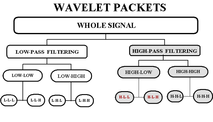
There are many wavelet packet libraries. They differ from each other by their generating filters and , the shape of the basic waveforms and their frequency content. In Fig. 10.17, we display the wavelet packets derived from the spline of 6-th order after decomposition into three scales. While the splines do not have a compact support in time domain, they are well localized. They produce perfect splitting of the frequency domain (see Fig. 10.17 right).
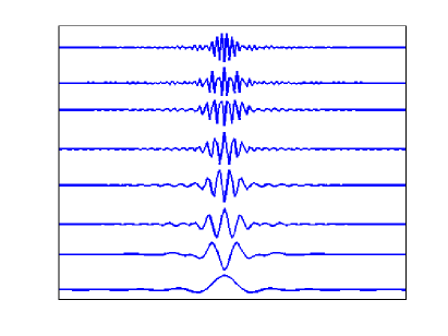
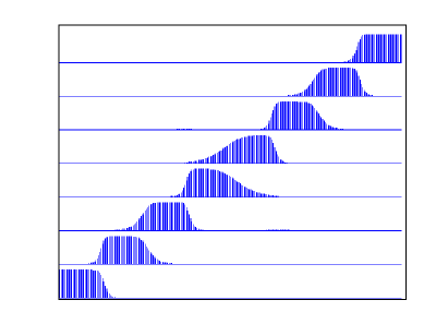
There is a duality in the nature of the wavelet coefficients of a certain block. On one hand, they indicate the presence of the corresponding waveform in the signal and measure its contribution. On the other hand, they evaluate the contents of the signal inside the related frequency bands. One may argue that the wavelet packet transform bridges the gap between time-domain and frequency-domain representations of a signal. As one advances into coarser level (scale), a better frequency resolution is seen at the expense of time domain resolution and vice versa. In principle, the transform of a signal of length can be implemented up to the -th decomposition level. At this level there exist different waveforms, which are close to the sine and cosine waves with multiple frequencies. In Fig. 10.18, we display a few wavelet packets derived from the spline of the 6-th order after decomposition into six levels. The waveforms resemble the windowed sine and cosine waves, whereas their spectra split the Nyquist frequency domain into 64 bands.
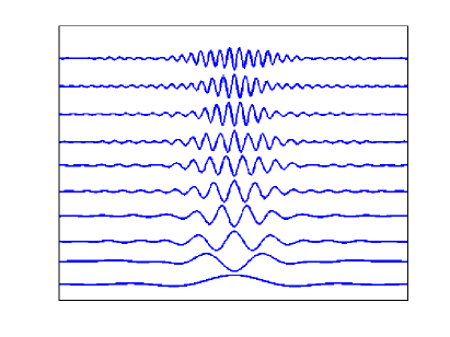
10.9 Appendix II: The Random Search for a Near Optimal FootPrint (RSNOFP) scheme
As mentioned above, three versions of the RSNOFP scheme are used:
- RSNOFP - version I:
-
A random matrix of size , where (typically, ) is created. Entries of the matrix are Gaussian random variables (see[64] for other options to choose ). The columns in the matrix are normalized. The matrix (defined in Section 10.5.2) is multiplied by the matrix . As a result, we obtain a new matrix of size . Each row in is associated with the corresponding slice from . This procedure reduces the dimensionality of the rows in by using the random projection scheme that was described in Section 2.2.
Next, we select the most significant columns (with respect to the average norm) of the matrix . Let
be the average norm of the j-Th column where and let be the vector of all averages. We denote by the set of indices of the largest coordinates of the vector (typically, ). Then, the columns, whose indices do not belong to , are removed from the matrix and the matrix of size is obtained. This operation is equivalent to multiplication of with the matrix of size , which is derived from by removing the rows, whose indices do not belong to . Thus, the initial matrix consisting of the V-class slices, whose size was, for example, , is reduced to the matrix of the random footprints of the slices. The size of is . To produce a similar reduction of the matrix of N-class slices, we multiply the N-class energy matrix with the matrix . As a result, we obtain the random footprints matrix of size . We consider the coordinates of the -th row of the matrices and as the set of characteristic features of the -th slice from the matrix and , respectively.
Next, we calculate the Mahalanobis distances , from each row in the V-class matrix to the matrix . We denote by
the average of the sequence .
The value is considered to be the distance between the feature sets and . The matrices , , and the value are stored and we proceed to optimize the features.
We repeat the above operations using a random matrix , whose structure is similar to the structure of the matrix . As a result, we obtain the feature matrices and , the random matrix and the distance value . The distance value is compared to the stored value . Assume, . This means that the features matrices and are better separated from one another than the stored matrices and . In this case, we replace the values in , , and by the values in , , and , respectively. If then the values in , , and are left intact.
We iterate this procedures up to 500 times. In the end, we stored the features matrices and such that the “distance" between them among all the iterations is maximal. We have stored the reduced random matrix and the pattern matrices and , which will be used in the identification phase. These items are denoted as , and .
- RSNOFP - Version II:
-
This version is similar, to some extent, to Version I. The difference is that, instead of selecting the most significant columns in the matrix , we apply the Principal Component Analysis (PCA) to this matrix. As a result, we obtain the matrix of size . Each column of contains the coefficients of one principal component. The columns are arranged in decreasing component variance order. The size of is reduced to by retaining only the first columns
We obtain the feature matrix for the V-class by multiplying by :
The size of the matrix is . Similarly, we produce the feature matrix for the N-class: . Similarly to Version I, we measure the “distance" between the feature sets and . The matrices , , and the value are stored and we proceed to optimization of the features, which is identical to Version I. Finally, we stored the features matrices and and the matrix . These items are denoted by , and .
- RSNOFP - version III:
-
This version differs from versions I and II. Here, we do not multiply the energy matrix by a random matrix but instead we perform a random permutation of the columns and retain the first columns. Thus, we get the matrix of size . Note, that this transform can be presented as the multiplication of the matrix by a matrix of size , , where each column consists of zeros except for one entry, which is equal to 1.
Example: Assume that the matrix is of size and corresponds to the permutation of the columns of a matrix of size while retaining the first three columns:The other operations are similar to the operations in Version II. We apply the PCA algorithm to the matrix , which results in the principal components matrix of size of coefficients of the principal components. The size of is reduced to by retaining only the first columns
We obtain the feature matrix for the V-class by multiplying by :
The size of the matrix is . We construct, in a similar manner, the feature matrix that corresponds to the N-class: . We measure the “distance" between the sets of features and . The matrices , , and the value are stored and we proceed to optimize the features, using the same procedure as in Versions I and II. Finally, the features matrices and and the matrix are stored. They are denoted as , and .
We illustrate the relations between the RSNOFP procedures (version II) by the diagram in Fig. 10.19.
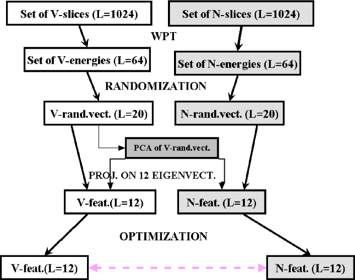
Chapter 11 Classification and Detection of High-Dimensional Medical Signals via Dimensionality Reduction
In this chapter, we introduce a generic approach which clusters and classifies datasets of acoustic signals. The proposed algorithms are robust to noise and to diverse recording conditions in which the signals were recorded. This methodology is able to detect different types of events.
Similarly to the algorithm in Chapter 10, the algorithms in this chapter consist of two steps: An offline training (learning) step that clusters the data and a detection step that classifies new data according to the clusters that were found in the first step. Different classes of events can be added to the training set and consequently to the detection phase.
We present two algorithms for clustering and classification. They apply a common feature extraction to the signals. However, the clustering procedure they use is different. One uses the diffusion maps algorithm (Chapter 3) and the other uses principle component analysis (Section 2.1). The proposed algorithms are generic and can be applied to various signal types for solving different classification problems. We demonstrate the generality of the algorithms on two different examples: detection of hypertension in adolescents and detection of abnormalities in heart beats. The robustness of the classification depends on the size and the quality of the training set.
This approach provides an alternative to the algorithm proposed in Chapter 9 while sharing a few common constructions.
11.1 Introduction
Clustering and classification of acoustic signals is a contemporary problem. This suggests a generic approach to cluster and classify datasets by discovering the geometric structure of the dataset. To achieve this, a training step embeds the training data into a low-dimensional space by using a dimensionality reduction scheme that preserves the geometrical structure of the dataset. Given a new high-dimensional data point for classification, it is first embedded into the low-dimensional space and its classification is determined according to its neighboring points in the low-dimensional space.
A preliminary step in the analysis of a signal is its decomposition into overlapping subsequences we refer to as windows. The resulting windows are regarded as data points in a high dimensional space where the dimensionality depends on the length of the subsequences. This high dimensional data contains dominating features along with redundancies. Consequently, the governing features need to be extracted while removing the redundancies. This is achieved by applying dimensionality reduction to the high dimensional data. The low dimensional space involves a small number of free parameters that convey the dominating features of the data.
The feature extraction procedures that are used in this chapter share the Spline Wavelet Packet Transform (Appendix I of Chapter 9) as a common preliminary step. However, they differ in the second step they use - one procedure uses the Diffusion Maps (Chapter 3) algorithm while the second uses Principal Component Analysis (Section 2.1).
The classification of acoustic signals is obtained via a two-phase process:
-
•
Learning phase (also referred to as training phase) in which data with a-priory classification is analyzed and features, which characterize it, are extracted and stored. The output of this phase is a separation of the input data into clusters, where each cluster represents a different class. learning phase is a one-time offline procedure.
-
•
Detection phase in which new data is classified using a feature database of known acoustic signatures. The detection phase is done in real-time (on-line) and the new data is classified according to the cluster it is the closest to (the Euclidean distance is minimal).
We illustrate the validity of these algorithms by using them to perform two detection tasks - each of which takes as input a different type of acoustic signals:
-
1.
Detection of early symptoms of arterial hypertension in adolescents.
-
2.
Detection of cardio-vascular diseases.
In both experiments 1 and 2 the algorithm should produce a minimal number of false detections. The classification of the data above is a difficult task since the pulses can vary significantly from one person to another. Providing an in-vivo solution to these medical detection problems is important since it enables to diagnose these diseases without the need of an invasive procedure. Furthermore, it can can be used for the diagnosis of other diseases by using acoustic signatures of the body such as pulse, as in the examples at hand, blood flow for the detection of various arterial diseases, abdominal sounds for the detection of gastrological problem, etc. In addition, the classification can be done in real-time.
Details of related works that tackle similar problems can be found in Section 9.2.
The rest of the chapter is organized as follows: The mathematical background on which the algorithm rely is given in Section 11.2. In Section 11.3 we present the main algorithms. The results of the two experiments are given in Section 11.4. Finally, in Section 11.5 we summarize the results and conclude this chapter.
11.2 Mathematical background
The proposed algorithms use various mathematical tools:
-
•
Spline wavelet - Similarly to Chapter 9, we extract features from the acoustic signals by applying the wavelet packet transform using spline wavelets of the sixth order (Battle-Lemarie [55]). The collection of energies in the blocks of wavelet packet coefficients constitutes the features of the signal. A description of the wavelet and wavelet-packet transforms is given in Chapter 9.
-
•
Principal component analysis - This is one of the two dimensionality reduction methods that are applied to the features after they were extracted. A description of this technique is given in Section 2.1.
-
•
Diffusion maps - This is the second dimensionality reduction method that is applied to the features after they were extracted. A description of this technique is given in Chapter 3.
-
•
Geometric harmonics - This is an out-of-sample extension scheme which we describe in details below. It is used to embed a new data point into the low-dimensional space during the real-time detection phase. The classification of the point is determined according to the class of the cluster which is the closest to it.
11.2.1 Geometric Harmonic (out-of-sample extension)
The geometric harmonic [131, 46, 132] provides a way to extend a known function on the learning set to a new point outside the sampling set, using both the target function and the geometry of the training set. A specific function that we extend is the low dimensional representation which is computed on the training set. This function is extended to data points outside the training set as part of the detection algorithm.
Let be a dataset and let be its diffusion embedding map as defined in Eq. 3.9 where and are the eigenvalues and eigenvectors, of the Gaussian kernel with width on the training data , respectively. We denote by the new dataset that includes the new data points to which we wish to extend . is the scale of extension.
The kernel can be evaluated in the entire space . Consequently, we get
where it is possible to use any on the right-hand-side of the identity.
The Nystrï¿œm extension [79] from of the eigenfunctions is given by:
| (11.1) |
Note that is being extended to a distance that is proportional to the distance from the new point to the training set .
Any function on the training set can be decomposed into
| (11.2) |
The Nystrï¿œm extension of on the rest of the space is given by:
| (11.3) |
The problem with this scheme is the choice of the kernel of extension. In the equations above, the same kernel that was used for the diffusion map embedding is used for the extension. Consequently, the functions will be extended to a distance that is proportional to the width of the Gaussian. However, when the diffusion embedding is computed, one strives to use as small a scale as possible, since the diffusion maps algorithm approximates the eigenvectors of the Laplace-Beltrami operator on the manifold and thus allows to discover the geometry of the underlying structure of the dataset. On the other hand, when extending a function, e.g. the diffusion coordinates outside the training set, one wants to be able to extend them as far as possible in order to maximize their generalization power. From the above it follows that the of the kernel, which is used for extending, should be as big as possible. This contradicts the strive for a small during the embedding process. Furthermore, this scale should not be the same for all functions we are trying to extend. Functions with large variations on should have a limited range of extension since it is more difficult to predict their values. As a result, one should adapt the scale of the extension to the function to be extended. Thus, the geometric harmonic algorithm uses two different kernels - one for the embedding with a small and another for the extension using a larger . We denote them by and , respectively. The eigenfunctions of the the embedding kernel constitute the functions we wish to extend and the eigenfunctions of the extension kernel are the ones that are used in Eq. 11.1. A procedure for finding an appropriate is described in [132].
11.3 Clustering and classification algorithms
The classification algorithms for processing acoustic signals consist of two phases: learning and detection. Two algorithms for clustering and classification are presented. These algorithms use the same procedure for feature extraction from a signal. However, they differ in the dimensionality reduction algorithms they employ. One uses the diffusion maps algorithm while the other uses PCA.
11.3.1 Preparation of the recorded datasets
The acoustics recordings are split into two sets: the training set which is used in phase I and the test set which is used in phase II.
Preparation of the acoustic recordings for the learning phase
The input data for the learning phase consists of acoustic signals given in a pulse-code modulation (PCM) format. The acoustic signals may have different sizes and their classifications are known a-priory. First, acoustics patterns are extracted from the input signals, where each pattern represents a single acoustic event. These events are then separated into classes, , where is the number of different classes (number of different types of events) in the dataset. In examples 1 and 2, are naturally determined as healthy and not healthy. Specifically, in example 2 is either normal heart beats or a vascular disease.
The number of patterns is given by . The training sample set recordings, whose classification is known a-priory, is denoted by , where each , represents an acoustic pattern from the training set. Each signal from the training set belongs to a class , .
Preparation of the recordings for the classification phase
In this phase, a signal from the testing set is divided into short segments. In the detection phase, each segment is processed and assigned to the most suitable class.
11.3.2 Learning phase
This phase contains two parts. The first part applies a feature extraction procedure to every signal and in the second part two methods of dimensionality reduction are used for clustering and classification of the training set to different classes.
Part I: Feature extraction
In order to extract the requires features from each signal, the following steps are employed:
- 1.
-
Decomposition into windows: Each acoustic signal is decomposed is decomposed into windows of size , , with overlapping of . The result is given by . We denote the classification of each window by .
- 2.
-
Application of spline wavelet: We use the sixth order spline wavelet packet. A spline wavelet is applied up to a scale on each window . Typically, if then and if then . The coefficients are taken from the last scale . This scale contains coefficients that are arranged into blocks of length . Each block is associated with a certain frequency band. These bands form a near uniform partition of the Nyquist frequency domain into parts. The output of this step is a set of spline wavelet coefficients for each window .
- 3.
-
Calculation of the energy: We construct the acoustic signature of a certain window using the distribution of energy among its wavelet packet coefficients. The energy is calculated by normalized sum of the coefficients in each block that was calculated in the previous step. Consequently, this step produces for each window a vector of size that contains the block energies of its wavelet packet coefficients. This operation reduces the dimension by a factor of .
- 4.
-
Averaging: This step is applied in order to reduce perturbations and noise. We calculate the average of every consecutive windows which are associated with the same signal in order to receive a more robust signature.
Part II: Dimensionality reduction of the learning set
After the features are extracted, we further reduce the dimensionality of the feature training set by applying two methods of dimensionality reduction: diffusion maps (Chapter 3) and PCA (Section 2.1). This step also clusters the data according to the a-priory classes.
Let , where is a vector of size , be the features extracted from the signal windows as described in Section 11.3.2. There are rows, each of size , where each row describes a fraction of a signal whose classification is known.
We apply the diffusion maps and PCA methods to and denote the produced low-dimensional embedding by and , respectively, where is of size . Thus, we achieve a dimensionality reduction from to . Since the PCA algorithm involves a step where the data is centered around the origin, we store the center of gravity of for the classification phase.
11.3.3 On-line classification phase
The classification phase is done on-line. There is no need to wait for the entire signal to be received. In order to classify a signal at time , the algorithm only needs the consecutive overlapping windows of size with overlap that immediately precede time . and are the same as in the learning phase. Given such a sequence, its classification is obtained by applying the following step:
-
1.
Feature extraction from the sequence giving a feature vector.
-
2.
Embedding of the feature vector into the low-dimensional space.
-
3.
Assignment of each window in the tested recording to a specific class.
The feature extraction that is used in the classification uses the same procedure as in the learning phase (Section 11.3.2). However, the second step depends on the method that was used for the dimensionality reduction. In case DM was used, the feature vector is embedded using the Geometric Harmonic algorithm (Section 11.2.1). Specifically, the embedding space is extended to contain the feature vector. If PCA was used, then the embedding of the feature vector is obtained by projecting it on the principal components (after reducing the center of gravity of the training set from the feature vector). The third step is the same for both dimensionality reduction schemes and is described below.
Classification of a new window
For each new embedded window (point), its nearest neighbors in the embedding space are found111We used the TSTOOL software from http://www.dpi.physik.uni-goettingen.de/tstool/ to find the nearest neighbors., where is given as a parameter. The classification is set according to the dominating class of the neighbors i.e. the class to which the largest number of neighbors belong. The classification probability is determined according to the ratio between the number of neighbors from the dominating class and .
11.4 Experimental results
We demonstrate the generality and the robustness of the algorithms using two the examples, we use the suggested algorithms with minor changes in the algorithms’ parameters which were determined empirically. The algorithms’ parameters are: - window size, - overlapping percent, - number of windows to average, - the scale of spline wavelet, - number of chosen eigenvalues in the DM algorithm.
The learning set was constructed as follows: we extracted from the recordings, which were assigned to the learning phase, fragments - each of which belongs to a certain known class.
The classification phase was tested on recordings that did not participate in the training set construction. For every recording that was processed in the classification phase, we provide graphs that include the following parts:
-
1.
The original signal.
-
2.
Graphs of the probabilities of the events that most likely took place according to the output of the DM-based classification algorithm.
-
3.
Graphs of the probabilities of the events that most likely took place according to the output of the PCA-based classification algorithm.
11.4.1 Experiment 1: Analyzing of radial artery pulse
The signals that were used in this experiment consisted of the radial artery pulse. This signals were captured at 200 seconds intervals by an optoelectronic sensor at a sampling rate of 100 Hz.
The classes that have to be separated are:
-
•
Hypertension.
-
•
Nocturnal enuresis
The data were collected from different children (ages 9-14) in different occasions. The training set contained 36 recordings and the detection set contained 2 recordings that did not take part in the learning phase. The following parameters were used in the learning and classification phases: , , , , .
The justification for using the spline wavelet packet is: the contribution of each oscillation inside the human body contains only a few dominating bands. As the conditions are changed the configuration of these bands may vary but the general disposition remains. From this we can assume that the signature for the class of pulse signals which are related to a certain disease, can be obtained as a combination of the inherent energies in a set of blocks of the wavelet packet coefficients of the decomposed signal.
Results from the learning phase
The clustering result from the DM algorithm is given in Fig. 11.1. The first three eigenvectors provide a complete separation into two disjoint clusters.
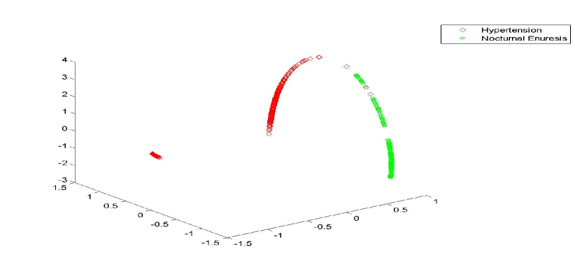
The clustering result from the PCA algorithm is given in Fig. 11.2. The first two eigenvectors provide a complete separation between the eigenvectors of the hypertension class (two clusters) and the eigenvectors of the nocturnal enuresis class (two clusters).
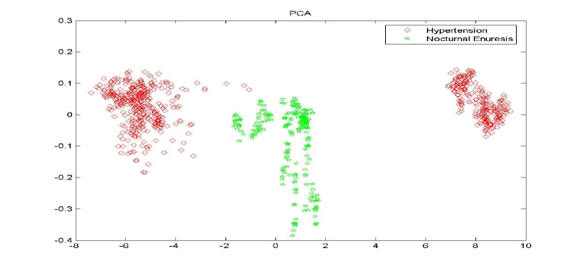
Results from the classification phase
Figure 11.3 contains the results of a hypertension signal that was not part of the training set. The blue line in the two bottom plots represents the detection probability of the DM and PCA algorithms of hypertension. It can be seen that they are both equal to one throughout the recording and thereby illustrating accurate classification since the signal belongs to a hypertensive patient. In Fig. 11.4 we see a fraction of the new signal embedded into the cluster that corresponds to the hypertension class.
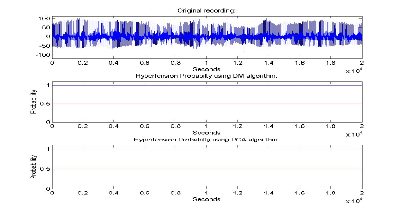
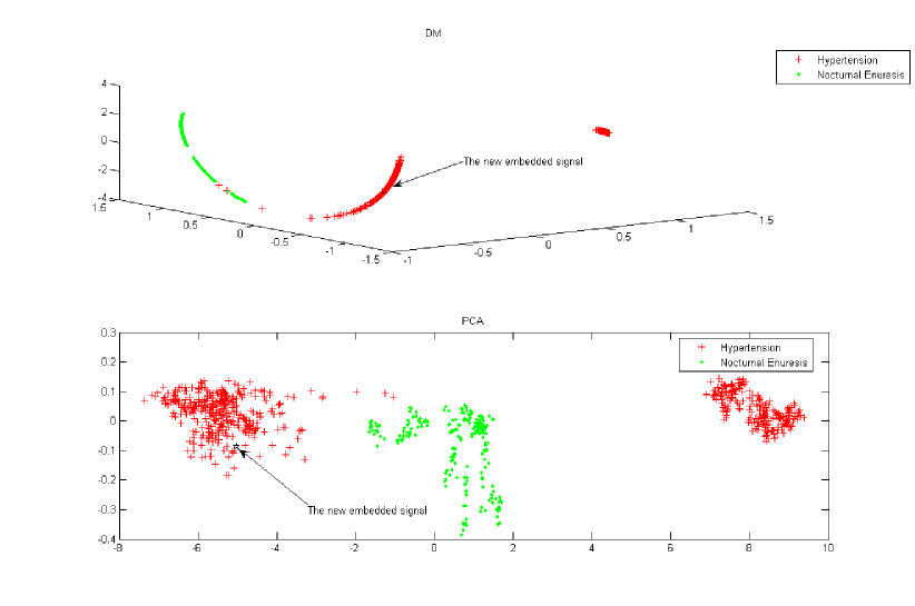
Figure 11.5 contains the classification results of a nocturnal enuresis signal. We see that in both algorithms the classification is accurate. In Fig. 11.6 we see that a fraction of the new signal embedded into the cluster that represents the nocturnal enuresis class.
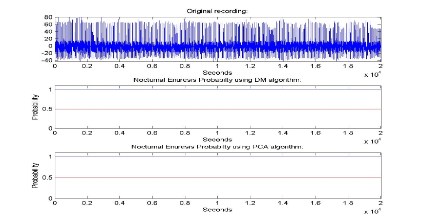
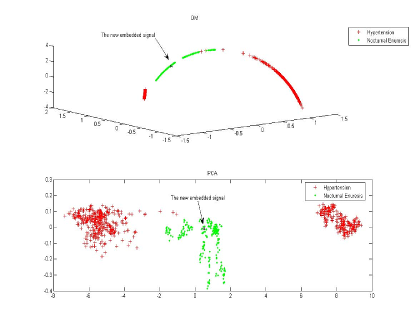
11.4.2 Experiment 2: Detection of a cardio vascular diseases
The signals for this experiment were obtained using a pulse detector working at sampling rates 22050 Hz and 11025 Hz. The signals were downsampled to 2205 Hz.
The classes in this experiment are: (a) normal heart beats and (b) a cardio vascular disease. The data were collected from different adults in different occasions. The learning sample set consisted of 7 recordings, 4 of them describe normal cardio behavior and 3 represent a cardio vascular disorder. The detection set contained 2 recordings that did not participate in the learning phase. The following parameters were used in the learning and classification phases: , , , , . These parameters were determined empirically.
Results from the learning phase
The clustering result of the PCA algorithm is given in Fig. 11.7. The first two eigenvectors provide a complete separation into two disjoint clusters. The clustering result of the DM algorithm is given in Fig. 11.8. The first two eigenvectors provide a complete separation into two disjoint clusters.
The clustering results obtained by both the PCA and the DM algorithms in this example are similar indicating that the manifold is close to linear in this case.
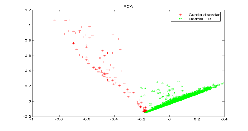
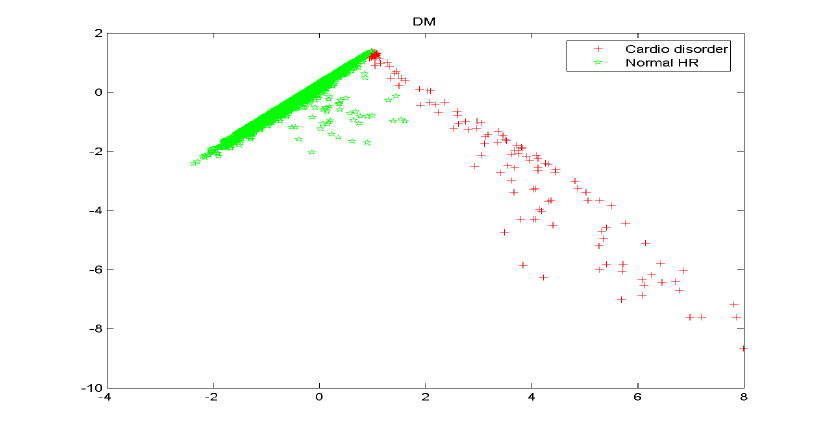
Results from the classification phase
Figure 11.9 contains the classification results of a cardio vascular disorder signal. DM and PCA provide clusters that classify the data accurately.
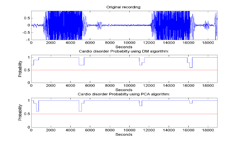
Figure 11.10 contains the classification results of a normal heart beat signal. Both the DM and the PCA algorithms classify the data accurately – they detect the abnormal heart beats and do not generate false detections.
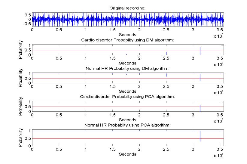
11.5 Conclusions
In this chapter, we introduced two algorithms for the detection of different types of events according to their acoustic signatures. Each algorithm has two phases. In both algorithms, dominating features were extracted from every acoustic signal (Section 11.3.2). In order to cluster different events, the features of the signals were embedded into a lower dimensional space using either the DM algorithm (Chapter 3) or the PCA algorithm (Section 2.1). In the on-line classification phase of new signals, acoustic dominating features were extracted from the signal by employing similar steps to the those that were used in the learning phase. The features of the new signal were embedded by using either the geometric harmonic scheme (in the DM algorithm) or a simple projection (in the PCA algorithm).
In the specific domain that was examined both algorithms perform very well where the PCA algorithm has a slight time complexity advantage. Nevertheless, when using the proposed schemes for other application domains, the accuracy of the PCA algorithm might be inferior to that of the DM algorithm due to its limiting capabilities in reducing the dimensionality of data-sets with a non-linear structure.
Chapter 12 Final Conclusions
In this thesis I introduced a novel method for dimensionality reduction - diffusion bases. The method is based on the diffusion map dimensionality reduction algorithm. I demonstrated the effectiveness of the method for the segmentation of images that originated from three different domains: hyper-spectral imagery, multi-contrast MRI and video. For each domain, a different algorithm was tailored in which the diffusion bases method was the key step that facilitated the generation of the results. These results were shown (where applicable) to be competitive with current state-of-the-art methods for the investigated problems.
In the second part of the thesis, I investigated dimensionality reduction as a tool for solving problems from various domains. Specifically, I used dimensionality reduction in order to uniquely characterize materials using their spectral signatures. I demonstrated how dimensionality reduction can be utilized for classification. I proposed an ensemble algorithm which incorporates three different dimensionality reduction techniques for the detection of vehicles. I also introduced two algorithms that use PCA and DM as tools for classification of medical signals. A clear conclusion can be made: dimensionality reduction proves to be a key tool in classification tasks. A question remains: “Which dimensionality reduction technique should be used ?”. The answer depends on the problem domain. Nevertheless, ensemble methods which apply several dimensionality reduction techniques might provide a more general solution than the application of any single technique.
I hope this thesis will trigger more research on the integration of dimensionality reduction for solving other problems in various other domains.
References
- [1] University of florida, college of medicine. a brief review of neuroanatomy. http://medinfo.ufl.edu/year2/neuro/review/index.html.
- [2] Aber, J. D., and Martin, M. E. High spectral resolution remote sensing of canopy chemistry. In Summaries of the Fifth JPL Airborne Earth Science Workshop, JPL Publication 95-1 (1995), vol. 1, pp. 1–4.
- [3] Afromowitz, M. A., Callis, J. B., and Heimbach, D. M. Multispectral imaging of burn wounds: a new clinical instrument for evaluating burn. IEEE Transactions on Biomedical Engineering 35, 10 (1988), 842–850.
- [4] Agrafiotis, D. K. Stochastic proximity embedding. Journal of Computational Chemistry 24, 10 (2003), 1215–1221.
- [5] Ashburner, J., and Friston, K. Multimodal image coregistration and partitioning - a unified framework. NeuroImage 6 (1997), 209–217.
- [6] Atkins, M. S., and Mackiewich, B. T. Fully automatic segmentation of the brain in MRI. IEEE Transactions on Medical Imaging 17 (1998), 98–107.
- [7] Averbuch, A., Ben-Gigi, N., Schclar, A., Zheludev, V., and Zur, Y. Automatic identification of features in hyperspectral data - construction of unique signatures: I. exact search. submitted to IEEE Transactions on Geosciences and Remote Sensing (2007).
- [8] Averbuch, A., Ben-Gigi, N., Schclar, A., Zheludev, V., and Zur, Y. Automatic identification of features in hyperspectral data - construction of unique signatures: II. approximate search. submitted to IEEE Transactions on Geosciences and Remote Sensing (2007).
- [9] Averbuch, A., Hulata, E., Zheludev, V., and Kozlov, I. A wavelet packet algorithm for classification and detection of moving vehicles. Multidimensional Systems and Signal Processing 12, 1 (2001), 9–31.
- [10] Averbuch, A., Kozlov, I., and Zheludev, V. Wavelet packet based algorithm for identification of quasi-periodic signals. In Proceedings of SPIE 4478, Wavelet Applications in Signal and Image Processing IX (2001), pp. 353–360.
- [11] Averbuch, A., and Zheludev, V. Wavelet and frame transforms originated from continuous and discrete splines. Advances in Signal Transforms: Theory and Applications (2006).
- [12] Averbuch, A., and Zheludev, V. Wavelet transforms generated by splines. to appear in International Journal of Wavelets, Multiresolution and Information Processing (2008).
- [13] Averbuch, A., Zheludev, V., Rabin, N., and Schclar, A. Wavelet based detection of moving vehicles. International Journal of Wavelets, Multiresolution and Information Processing http://dx.doi.org/10.1007/s11045-008-0058-z (2008).
- [14] Beghdadi, A., and Negrate, A. L. Contrast enhancement technique based on local detection of edges. Computer Vision Graphics Image Processing 46 (1989), 162–174.
- [15] Belkin, M., and Niyogi, P. Laplacian eigenmaps for dimensionality reduction and data representation. Neural Computation 15, 6 (2003), 1373–1396.
- [16] Bellman, R. Adaptive control process: a guided tour. Princeton University Press, 1961.
- [17] Belongie, S., Fowlkes, C., Chung, F., and Malik, J. Spectral partitioning with indefinite kernels using the Nyström extension. In Proceedings of the 7th European Conference on Computer Vision-Part III (2002), Springer-Verlag, pp. 531–542.
- [18] Ben-Dor, E., Patin, K., Banin, A., and Karnieli, A. Mapping of several soil properties using dais-7915 hyperspectral scanner data. a case study over clayey soils in Israel. International Journal of Remote Sensing (in press) (2001).
- [19] Bendersky, M., Rugilo, C., Kochen, S., Schuster, G., and Sica, R. E. P. Magnetic resonance imaging identifies cytoarchitectonic subtypes of the normal human cerebral cortex. Journal of Neurological Science 211 (2003), 75–80.
- [20] Beyer, K. S., Goldstein, J., Ramakrishnan, R., and Shaft, U. When is ”nearest neighbor” meaningful? In Proceedings of the 7th international Conference on Database theory (London, January 1999), C. Beeri and P. Buneman, Eds., vol. 1540 of Lecture Notes In Computer Science, Springer-Verlag, pp. 217–235.
- [21] Bishop, C. M., Svenson, M., and Computation, C. K. I. W. N. Gtm: The generative topographic mapping. Neural Computation 10, 1 (1998), 215–234.
- [22] Blinkenberg, M., Rune, K., Jensen, C. V., Ravnborg, M., Kyllingsbaek, S., Holm, S., Paulson, O., and Sorensen, P. Cortical cerebral metabolism correlates with MRI lesion load and cognitive dysfunction in MS. Neurology 54 (2000), 558–564.
- [23] Bourgain, J. On lipschitz embedding of finite metric spaces in Hilbert space. Israel Journal of Mathematics 52 (1985), 46–52.
- [24] Brand, M. Charting a manifold. In Advances in Neural Information Processing Systems, vol. 15. The MIT Press, Cambridge, MA, USA, 2002, pp. 985–992.
- [25] Brand, M. From subspaces to submanifolds. In Proceedings of the 15th British Machine Vision Conference (London, UK, 2004), British Machine Vision Association.
- [26] Breiman, L., Friedman, J. H., Olshen, R. A., and Stone, C. J. Classification and Regression Trees. Chapman & Hall, Inc., New York, 1993.
- [27] Bronstein, A. M., Bronstein, M. M., and Kimmel, R. Generalized multidimensional scaling: a framework for isometry-invariant partial surface matching. In Proceedings of the National Academy of Sciences (PNAS) (2006), vol. 103(5), pp. 1168–1172.
- [28] Buchsbaum, M. S., Byne, W., Hazlett, E. A., Shihabuddin, L., Tang, C. Y., Wei, T. C., Haznedar, M., and Siever, L. J. PET, MRI, and postmortem studies of the thalamus in schizophrenia. In Proceedings of the Fifth International Conference on Functional Mapping of the Human Brain (1999), p. 639.
- [29] Cancio, L. C., Brand, D. D., and Kerby, J. Visible hyperspectral imaging: monitoring the systemic effects of shock and resuscitation. In Proceedings of SPIE (2002), vol. 4614, pp. 159–168.
- [30] Candès, E., Romberg, J., and Tao, T. Robust uncertainty principles: Exact signal reconstruction from highly incomplete frequency information. IEEE Transactions on Information Theory 52, 2 (February 2006), 489–509.
- [31] Carvalho, O. A. J., Carvalho, A. P., Meneses, P. R., and Guimaraes, R. F. Spectral identification method (SIM): A new classifier based on the ANOVA and spectral correlation mapper (SCM) methods. In AVIRIS Proceedings, JPL Publication (2001).
- [32] Carvalho, O. A. J., Guimares, R. F., Carvalho, A. P., Silva, N. C., Martins, E. S., and Gomes, R. A. T. Vegetation mapping in the Parque Nacional, Brasilia (Brazil) area using advanced spaceborne thermal emission and reflection radiometer (ASTER) data and spectral identification method (SIM). In Remote Sensing for Environmental Monitoring, GIS Applications, and Geology V. Proceedings of the SPIE, 5983 (2005), pp. 45–55.
- [33] Carvalho, O. A. J., and Meneses, P. R. Spectral correlation mapper (SCM): An improvement on the Spectral Angle Mapper. In Ninth JPL Airborne Earth Science Workshop. JPL Publication 00-18 (2000), pp. 65–74.
- [34] Chan, T. F., and Vese, L. A. Active contours without edges. IEEE Transactions On Image Processing 10, 2 (February 2001), 266–275.
- [35] Chang, H., Yeung, D. Y., and Xiong, Y. Super-resolution through neighbor embedding. In IEEE Computer Society Conference on Computer Vision and Pattern Recognition (2004), vol. 1, pp. 275–282.
- [36] Chang, K. Y., and Ghosh, J. Principal curves for nonlinear feature extraction and classification. In Applications of Artificial Neural Networks in Image Processing III. SPIE, Bellingham, WA, USA, 1998, pp. 120–129.
- [37] Chang, Y. L., and Li, X. Adaptive image region-growing. IEEE Transactions on Image Processing 3, 6 (1994), 868–872.
- [38] Chavez, P. S. J., Guptill, C., and Bowel, J. A. Image processing techniques for thematic mapper data. In Proceeding of the American Society of photogrametry Conference (Washington, 1984), pp. 728–752.
- [39] Choe, H. C., Karlsen, R. E., Meitzler, T., Gerhart, G. R., and Gorsich, D. Wavelet-based ground vehicle recognition using acoustic signals. Proceedings of the SPIE, 2762:434-445 (1996).
- [40] Choi, H., and Choi, S. Robust kernel Isomap. Pattern Recognition 40, 3 (2007), 853–862.
- [41] Chung, F. R. K. Spectral Graph Theory. AMS Regional Conference Series in Mathematics, 92, 1997.
- [42] Clark, R. N., and Swayze, G. A. Mapping minerals, amorphous materials, environmental materials, vegetation, water, ice and snow, and other materials: The USGS tricorder algorithm. In Proceedings of the Fifth JPL Airborne Earth Science Workshop, JPL Publication 95-1 (1995), vol. 1, pp. 39–40.
- [43] Clark, R. N., Swayze, G. A., and Gallagher, A. Mapping the mineralogy and lithology of canyonlands, Utah with imaging spectrometer data and the multiplespectral feature mapping algorithm. In Summaries of the Third Annual JPL Airborne Geoscience Workshop, JPL Publication, 92-14 (1992), vol. 1, pp. 11–13.
- [44] Clark, R. N., Swayze, G. A., and King, T. V. V. Imaging spectroscopy: A tool for earth and planetary system science remote sensing with the USGS tetracorder algorithm. Journal of Geophysical Research (2001).
- [45] Coifman, R. R., and Lafon, S. Diffusion maps. Applied and Computational Harmonic Analysis: special issue on Diffusion Maps and Wavelets 21 (July 2006), 5–30.
- [46] Coifman, R. R., and Lafon, S. Geometric harmonics: a novel tool for multiscale out-of-sample extension of empirical functions. Applied and Computational Harmonic Analysis: special issue on Diffusion Maps and Wavelets 21 (July 2006), 31–52.
- [47] Coifman, R. R., Lafon, S., Lee, A., Maggioni, M., Nadler, B., Warner, F., and Zucker, S. Geometric diffusions as a tool for harmonics analysis and structure definition of data: Diffusion maps. In Proceedings of the National Academy of Sciences (May 2005), vol. 102, pp. 7432–7437.
- [48] Coifman, R. R., Meyer, Y., and Wickerhauser, M. V. Adapted waveform analysis, wavelet-packets, and applications. In Proceedings of the ICIAM’91 (Philadelphia, 1991), SIAM Press.
- [49] Comaniciu, D. An algorithm for data-driven bandwidth selection. IEEE Transanctions on Pattern Analysis and Machine Intelligence 25, 2 (2003), 281–288.
- [50] Comaniciu, D., and Meer, P. Mean shift a robust approach toward feature space analysis. IEEE Transanctions on Pattern Analysis and Machine Intelligence 24, 5 (2002), 603–619.
- [51] Combarros, O., Miro, J., and Berciano, J. Ageusia associated with thalamic plaque in multiple sclerosis. European Neurology 34 (1994), 344–346.
- [52] Cox, T., and Cox, M. Multidimensional scaling. Chapman & Hall, London, UK, 1994.
- [53] Criqui, M. H., Coughlin, S. S., and Fronek., A. Noninvasively diagnosed peripheral arterial disease as a predictor of mortality: Results from a prospective study. Circulation 72 (1985), 768–773.
- [54] Cucchiara, R., Grana, C., Piccardi, M., and Prati, A. Detecting moving objects, ghosts, and shadows in video streams. IEEE Transactions on Pattern Analysis and Machine Intelligence 25, 10 (2003), 1337–1442.
- [55] Daubechies, I. Ten Lectures on Wavelets. SIAM, 1992.
- [56] Davis, G. L., Maggioni, M., Warner, F. J., Geshwind, F. B., Coppi, A. C., DeVerse, R. A., and Coifman, R. R. Spectral analysis of normal and malignant microarray tissue sections using a novel micro-optoelectrial mechanical system. Modern Pathology 17 (2004), 1:358A.
- [57] Davis, J. C. Statistics and Data Analysis in Geology. John Wiley & Sons, Inc., New York, NY, USA, 1973.
- [58] Davis, K. D., Kwan, C. L., Crawley, A. P., and Mikulis, D. J. Functional MRI study of thalamic and cortical activations evoked by cutatenous heat, cold, and tactile stimuli. Journal of Neurophysics 80 (1998), 1533–1546.
- [59] DeMers, D., and Cottrell, G. Non-linear dimensionality reduction. In Advances in Neural Information Processing Systems, vol. 5. Morgan Kaufmann, San Mateo, CA, USA, 1993, pp. 580–587.
- [60] Dhawan, A. P., Buelloni, G., and Gordon, R. Enhancement of mammographic features by optimal adaptive neighborhood image processing. IEEE Transactions on Medical Imaging 5 (1986), 8–15.
- [61] Dhawan, A. P., and Gordon, R. Reply to comments on enhancement of mammographic features by optimal adaptive neighborhood image processing. IEEE Transactions on Medical Imaging 6 (1987), 82–83.
- [62] Dhawan, A. P., and Royer, E. L. Mammographic feature enhancement by computerized image processing. Computer Methods and Programs in Biomedicine 27 (1988), 23–35.
- [63] Dijkstra, E. W. A note on two problems in connexion with graphs. Numerische Mathematik 1 (1959), 269–271.
- [64] Donoho, D., and Tsaig, Y. Extensions of compressed sensing. Signal Processing 86, 3 (March 2006), 533–548.
- [65] Donoho, D. L. Nonlinear wavelet methods for recovery of signals, densities, and spectra from indirect and noisy data. Proceedings of Symposia in Applied Mathematics 47 (1993), 173–205.
- [66] Donoho, D. L. Denoising via soft thresholding. IEEE Transactions on Information Theory 41 (1995), 613–627.
- [67] Donoho, D. L. Compressed sensing. IEEE Transactions on Information Theory 52, 4 (April 2006), 1289–1306.
- [68] Donoho, D. L., and Grimes, C. Hessian eigenmaps: new locally linear embedding techniques for high-dimensional data. In Proceedings of the National Academy of Sciences (May 2003), vol. 100(10), pp. 5591–5596.
- [69] Duraiswami, R., and Raykar, V. C. The manifolds of spatial hearing. In Proceedings of International Conference on Acoustics, Speech and Signal Processing (2005), vol. 3, pp. 285–288.
- [70] Duvernoy, H. The Human Brain. Surface, Three-Dimensional Sectional Anatomy and MRI. Springer-Verlag, New York, 1991.
- [71] Elgammal, A., Hanvood, D., and Davis, L. S. Nonparametric model for background subtraction. Proceedings of the European Conference on Computer Vision 2000 (June 2000), 751–767.
- [72] Elvidge, C. D. Visible and infrared reflectance characteristics of dry plant materials. International Journal of Remote Sensing 11, 10 (1990), 1775–1795.
- [73] Eom, K. B. Analysis of acoustic signatures from moving vehicles using time-varying autoregressive models. Multidimensional Systems and Signal Processing 10 (1999), 357–378.
- [74] Everitt, B. S., Landau, S., and Leese, M. Cluster Analysis. Arnold, London, 2001.
- [75] Faloutsos, C., and Lin, K. I. Fastmap: A fast algorithm for indexing, data-mining and visualization of traditional and multimedia datasets. In Proceedings of the 1995 ACM SIGMOD International Conference on Management of Data (New York, NY, USA, 1995), ACM Press, pp. 163–174.
- [76] Fatterpekar, G. M., Naidich, T. P., Delman, B. N., Aguinalso, J. G., Gultekin, S. H., Sherwood, C. C., Hof, P. R., Drayer, B. P., and Fayad, Z. A. Cytoarchitecture of the human cerebral cortex: MR microscopy of excised specimens at 9.4 Tesla. American Journal of Neuroradiology 23 (2002), 1313–1321.
- [77] Fisher, R. A. The use of multiple measurements in taxonomic problems. Annals of Eugenics 7 (1936), 179–188.
- [78] Floyd, R. W. Algorithm 97: Shortest path. Communications of the ACM 5, 6 (1962), 345.
- [79] Fowlkes, C., Belongie, S., Chung, F., and Malik, J. Spectral grouping using the Nyström method. IEEE Transactions on Pattern Analysis and Machine Intelligence 26, 2 (2004), 214–225.
- [80] Fowlkes, C., Belongie, S., and Malik, J. Efficient spatiotemporal grouping using the Nyström method. In CVPR, Hawaii (December 2001).
- [81] Frei, W. Image enhancement by histogram hyperbolization. Computer Graphics and Image Processing 6 (1977), 286–294.
- [82] Giroux, M. L., Grafton, S. T., Votaw, J. R., DeLong, M. L., and Hoffman, J. M. Medication related changes in cerebral glucose metabolism in Parkinsons disease. In Proceedings of the Fourth International Conference on Functional Mapping of the Human Brain (1998), p. 237.
- [83] Gonzalez, R. C., and Woods, R. E. Digital Image Processing, second ed. Prentice Hall, New Jersey, 2002.
- [84] Gorden, R., and Rangayyan, R. M. Feature enhancement of film mammograms using fixed and adaptive neighborhoods. Applied Optics 23 (1984), 560–564.
- [85] Graepel, T., and Computation, K. O. N. A stochastic self-organizing map for proximity data. Neural Computation 11, 1 (1999), 139–155.
- [86] Gromov, M. Structures métriques pour les variétés riemanniennes. CEDIC, Paris, 1981.
- [87] Grove, C. I., Hook, S. J., and Paylor, E. D. Laboratory reflectance spectra for 160 minerals 0.4 - 2.5 micrometers. In JPL Publication 92-2 (1992).
- [88] Han, B., Comaniciu, D., and Davis, L. S. Sequential kernel density approximation through mode propagation: applications to background modeling. Proceedings of the Asian Conference on Computer Vision (Jan. 2004).
- [89] Han, J., and Kamber, M. Data Mining. Morgan Kaufmann Publishers, 2001.
- [90] Hardy, A. On the number of clusters. Computational Statistics and Data Analysis 28 (1996), 83–96.
- [91] He, X., and Niyogi, P. Locality preserving projections. In Advances in Neural Information Processing Systems, vol. 16. The MIT Press, Cambridge, MA, USA, 2004, p. p37.
- [92] He, X., Yan, S., Hu, Y., Niyogi, P., and Zhang, H. J. Face recognition using Laplacianfaces. IEEE Transactions on Pattern Analysis and Machine Intelligence 27, 3 (2005), 328–340.
- [93] Heckers, S., Curran, T., Goff, D., Rauch, S. L., Fischman, A. J., Alpert, N. M., and Schacter, D. L. Abnormalities in the thalamus and prefrontal cortex during episodic object recognition in schizophrenia. Biological Psychiatry 48 (2000), 651–657.
- [94] Hein, M., and Audibert, Y. Intrinsic dimensionality estimation of submanifolds in Euclidean space. In Proceedings of the 22nd International Conference on Machine Learning (2005), pp. 289–296.
- [95] Hinton, G. E., Osindero, S., and Teh, Y. A fast learning algorithm for deep belief nets. Neural Computation 18, 7 (2006), 1527–1554.
- [96] Hinton, G. E., and Roweis, S. T. Stochastic neighbor embedding. In Advances in Neural Information Processing Systems, vol. 15. The MIT Press, Cambridge, MA, USA, 2002, pp. 833–840.
- [97] Hinton, G. E., and Salakhutdinov, R. R. Reducing the dimensionality of data with neural networks. Science 313, 5786 (2006), 504–507.
- [98] Hoffmann, H. Kernel PCA for novelty detection. Pattern Recognition 40, 3 (2007), 863–874.
- [99] Holland, J. H. Adaptation in Natural and Artificial Systems. University of Michigan Press, Ann Arbor, MI, USA, 1975.
- [100] Honkela, T., Kaski, S., Lagus, K., and Kohonen, T. Websom self-organizing maps of document collections. In WSO97 - Workshop on Self-Organizing Maps (Epsoo, Finland, June 1997), pp. 310–315.
- [101] Horowitz, S. L., and Pavlidis, T. Picture segmentation by a directed split-and-merge procedure. In Proceedings of the 2nd Int. Joint Conference on Pattern Recognition (Copenhagen, Denmark, 1974), pp. 424–433.
- [102] Hosel, V., and Walcher, S. Clustering techniques: A brief survey. Tech. rep., Institute of Biomathematics and Biometry, Neuherberg, Germany, 2001.
- [103] Hotelling, H. Analysis of a complex of statistical variables into principal components. Journal of Educational Psychology 24 (1933), 417–441.
- [104] Huber, P. J. Robust Statistics. John Wiley & Sons, 1981.
- [105] Huber, R., Ramoser, H., Mayer, K., Penz, H., and Rubik, M. Classification of coins using an eigenspace approach. Pattern Recognition Letters 26, 1 (2005), 61–75.
- [106] Hummel, R. Histogram modification techniques. Computer Graphics and Image Processing 4 (1975), 209–224.
- [107] Inselberg, A. The plane with parallel coordinates. The Visual Computer 1 (1985), 69–91.
- [108] Jenkins, O. C., and Mataric, M. J. Deriving action and behavior primitives from human motion data. In International Conference on Intelligent Robots and Systems (2002), vol. 3, pp. 2551–2556.
- [109] Jensen, J. Introductory Digital Image Processing. Prentice Hall, New Jersey, 1986.
- [110] Jimenez, L. O., and Landgrebe, D. A. Supervised classification in high-dimensional space: geometrical, statistical and asymptotical properties of multivariate data. IEEE Transactions on Systems, Man and Cybernetics, Part C: Applications and Reviews, 28, 1 (February 1998), 39–54.
- [111] Johnson, W. B., and Lindenstrauss, J. Extensions of Lipshitz mapping into Hilbert space. Contemporary Mathematics 26 (1984), 189–206.
- [112] Jonasson, L., Hagmann, P., Wilson, C. R., Bresson, X., Pollo, C., Meuli, R., and Thiran, J.-P. Coupled region-based level sets for segmentation of the thalamus and its subnuclei in DT-MRI. In Proceedings of 13th Annual Meeting (ISMRM) (Miami, 2005), p. 731.
- [113] Kass, M., Witkin, A., and Terzopolous, D. Snakes: Active contour models. In International Conference on Computer Vision (London, 1987), pp. 259–268.
- [114] Kaufman, L., and Rousseeuw, P. Finding Groups in Data: An Introduction to Cluster Analysis. John Wiley, New York, 1990.
- [115] Kellicut, D. C., Weiswasser, J. M., Arora, S., Freeman, J. E., Lew, R. A., Shuman, C., Mansfield, J. R., and Sidawy, A. N. Emerging technology: Hyperspectral imaging. Perspectives in Vascular Surgery and Endovascular Therapy 16, 1 (2004), 53–57.
- [116] Kikinis, R., Shenton, M. E., Iosifescu, D. V., McCarley, R. W., Saiviroonporn, P., Hokama, H. H., Robatino, A., Metcalf, D., Wible, C. G., Portas, C. M., Donnino, R. M., and Jolesz, F. A. A digital brain atlas for surgical planning, model-driven segmentation, and teaching. IEEE Transactions on Visualization and Computer Graphics 2 (1996), 232–241.
- [117] Kim, K. I., Jung, K., and Kim, H. J. Face recognition using kernel principal component analysis. IEEE Signal Processing Letters 9, 2 (2002), 40–42.
- [118] Kirkpatrick, S., Gelatt, C. D., and Vecchi, M. P. Optimization by simulated annealing. Science 220, 4598 (1983), 671–680.
- [119] Kogan, J., Nicholas, C., and Teboulle, M. Grouping Multidimensional Data: Recent Advances in Clustering. Springer-Verlag, Berlin, 2005.
- [120] Kohonen, T. Self-Organizing Maps, vol. 30 of Springer Series in Information Sciences. Springer, Berlin, 2001.
- [121] Koller, D., Weber, J. W., and Malik, J. Robust multiple car tracking with occlusion reasoning. European Conference on Computer Vision (1994).
- [122] Kong, S. G., Du, Z., Martin, M., and Vo-Dinh, T. Hyperspectral fluorescence image analysis for use in medical diagnostics. In Advanced Biomedical and Clinical Diagnostic Systems III. Proceedings of the SPIE (2005), vol. 5692, pp. 21–28.
- [123] Korb, A. R., Dybwad, P., Wadsworth, W., and Salisbury, J. W. Portable FTIR spectrometer for field measurements of radiance and emissivity. Applied Optics 35 (1996), 1679–1692.
- [124] Kotsiantis, S., and Pintelas, P. Recent advances in clustering: A brief survey. WSEAS Transactions on Information Science and Applications 1, 1 (2004), 73–81.
- [125] Kruggel, F., Bruckner, M. K., Arendt, T., Wiggins, C. J., and von Cramon, D. Y. Analyzing the neocortical fine-structure. Medical Image Analysis 7 (September 2003), 251–264.
- [126] Kruse, F. A., Lefkoff, A. B., Boardman, J. W., Heiehbrecht, K. B., Shapiro, A. T., Barloon, P. J., and Goetz, A. F. H. The Spectral Image Processing Software - (SIPS) for integrated analysis of AVIRIS data. In Summaries of the 4th Annual JPL Airborne Geosciences Workshop, JPL Publication 92-14 (1992), pp. 23–25.
- [127] Kruse, F. A., Lefkoff, A. B., Boardman, J. W., Heiehbrecht, K. B., Shapiro, A. T., Barloon, P. J., and Goetz, A. F. H. The spectral image processing system (SIPS) - interactive visualization and analysis of imaging spectrometer data. Remote Sensing of Environment 44 (1993), 145–163.
- [128] Kruse, F. A., Lefkoff, A. B., and Dietz, J. B. Expert system-based mineral mapping in North Death Valley, California/Navada, using the airborne visible/infrared imaging spectrometer (AVIRIS). Remote Sensing of Environment 44 (1993), 309–336.
- [129] Kruskal, J. B. Multidimensional scaling by optimizing goodness of fit to a nonmetric hypothesis. Psychometrika 29 (1964), 1–27.
- [130] Kung, S. Y., Diamantaras, K. I., and Taur, J. S. Adaptive principal component extraction (APEX) and applications. IEEE Transactions on Signal Processing 42, 5 (1994), 1202–1217.
- [131] Lafon, S. Diffusion maps and geometric harmonics. PhD thesis, Yale University, Dept of Mathematics and Applied Mathematics, May 2004.
- [132] Lafon, S., Keller, Y., and Coifman, R. R. Data fusion and multi-cue data matching by diffusion maps. IEEE Transactions on Pattern Analysis and Machine Intelligence 28, 11 (2006), 1784–1797.
- [133] Lafon, S., and Lee, A. Diffusion maps and coarse-graining: A unified framework for dimensionality reduction, graph partitioning, and data set parameterization. IEEE Transactions on Pattern Analysis and Machine Intelligence 28, 9 (September 2006), 1393–1403.
- [134] Laine, A., Fan, J., and Yang, W. Wavelets for contrast enhancement of digital mammography. IEEE Engineering in Medicine and Biology Magazine 14, 5 (1995), 536–550.
- [135] Lee, J. A., and Verleysen, M. Nonlinear dimensionality reduction of data manifolds with essential loops. Neurocomputing 67 (2005), 29–53.
- [136] Lemieux, L., Hammers, A., Mackinnon, T., and Lie, R. S. Automatic segmentation of the brain and intracranial cerebrospinal fluid in T1-weighted volume MRI scans of the head, and its application to serial cerebral and intracranial volumetry. Magnetic Resonance in Medicine 49 (2003), 872–884.
- [137] Lim, I. S., Ciechomski, P. H., Sarni, S., and Thalmann, D. Planar arrangement of high-dimensional biomedical data sets by Isomap coordinates. In Proceedings of the 16th IEEE Symposium on Computer-Based Medical Systems (2003), pp. 50–55.
- [138] Lima, A., Zen, H., Nankaku, Y., Miyajima, C., Tokuda, K., and Kitamura, T. On the use of Kernel PCA for feature extraction in speech recognition. IEICE Transactions on Information Systems E87-D, 12 (2004), 2802–2811.
- [139] Linial, M., Linial, N., Tishby, N., and Yona, G. Global self-organization of all known protein sequences reveals inherent biological signatures. Journal of Molecular Biology 268, 2 (May 1997), 539–556.
- [140] Lipton, R. C. A., and Kanade, T. Introduction to the special section on video surveillance. IEEE Transactions on Pattern Analysis and Machine Intelligence 22, 8 (Aug. 2000), 745 – 746.
- [141] Lo, B., and Velastin, S. Automatic congestion detection system for underground platforms. Proceedings of ISIMP2001 (May 2001), 158–161.
- [142] Macivor, A. Background subtraction techniques. Proceedings of Image and Vision Computing (2000).
- [143] MacQueen, J. B. Some methods for classification and analysis of multivariate observations. In Proceedings of 5th Berkley Symposium on Mathematical Statistics and Probability (1967), vol. 1 Statistics, pp. 281–297.
- [144] Maggioni, M., Warner, F. J., Davis, G. L., Coifman, R. R., Geshwind, F. B., Coppi, A. C., and DeVerse, R. A. Hyperspectral microscopic analysis of normal, adenoma and carcinoma microarray tissue sections. SPIE Optical Biopsy 6091, 60910I (2006).
- [145] Maggioni, M., Warner, F. J., Davis, G. L., Coifman, R. R., Geshwind, F. B., Coppiand, A. C., and DeVerse, R. A. Algorithms from signal and data processing applied to hyperspectral analysis: Application to discriminating normal and malignant microarray colon tissue sections. Tech. rep., Yale University, Department of Computer Science, February 2004.
- [146] Magnotta, V. A., Gold, S., Andreasen, N. C., Ehrhardt, J. C., and Yuh, W. T. Visualization of subthalamic nuclei with cortex attenuated inversion recovery MR imaging. NeuroImage 11 (2000), 341–346.
- [147] Maimon, O., and Rokach, L., Eds. The Data Mining and Knowledge Discovery Handbook: A Complete Guide for Practitioners and Researchers. Springer, 2005.
- [148] Mallat, S. A Wavelet Tour of Signal Processing, second ed. Academic Press, New York, 1998.
- [149] Mansfield, J. R., Sowa, M. G., and Payette, J. A fuzzy cmeans clustering approach to the analysis of multispectral images of the rat dorsal skin flap. IEEE Transactions on Medical Imaging 6 (1998), 1011–1018.
- [150] Mardia, K. V., Kent, J. T., and Bibby, J. M. Multivariate Analysis. Academic Press, London, 1979.
- [151] Marrett, S., Danek, A., Vortmeyer, A., Van-Gelderen, P., Duyn, J., Bandettini, P., Gtafman, J., and Koretsky, A. P. Imaging cortical anatomy by high-resolution MR at 3.0T: Detection of the stripe of Gennari in visual area 17. Magnetic Resonance in Medicine 48, 4 (2002), 735–738.
- [152] Merton, R. N. Multi-temporal analysis of community scale vegetation stress with imaging spectroscopy. PhD thesis, Geography Department, University of Auckland, New Zealand, 1999.
- [153] Monteiro, S. T., Kosugi, Y., Uto, K., and Watanabe, E. Towards applying hyperspectral imagery as an intraoperative visual aid tool. In Proceedings of the 4th Conference on Visualization, Imaging, and Image Processing (VIIP) (Marbella, Spain, 2004), pp. 483–488.
- [154] Morel, A., Magnin, M., and Jeanmonod, D. Multiarchitectonic and stereotactic atlas of the human thalamus. The Journal of Comparative Neurology 387 (1997), 588–630.
- [155] Mumford, D., and Shah, J. Optimal approximations by piecewise smooth functionsand associated variational problems. Communications On Pure and Applied Mathematics 42 (1989), 577–685.
- [156] Munich, M. E. Bayesian subspace method for acoustic signature recognition of vehicles. Proceedings of the 12th European Signal Processing Conference EUSIPCO (2004).
- [157] Navon, E., Miller, O., and Averbuch, A. Z. Color image segmentation based on adaptive local thresholds. Image and Vision Computing 23, 1 (January 2004), 69–85.
- [158] Ng, A., Jordan, M., and Weiss, Y. On spectral clustering: Analysis and an algorithm. In Advances in Neural Information Processing Systems, vol. 14. The MIT Press, Cambridge, MA, USA, 2001, pp. 849–856.
- [159] Niemann, K., Mennicken, V. R., Jeanmonod, D., and Morel, A. The Morel stereotactic atlas of the human thalamus: atlas-to-MR registration of internally consistent canonical model. NeuroImage 12 (2000), 601–616.
- [160] öAyrämö, S. Knowledge mining using robust clustering. PhD thesis, University of Jyväskylä, 2006.
- [161] Ogawa, T., Yoshida, Y., Okudera, T., Noguchi, K., Kado, H., and Uemura, K. Secondary thalamic degeneration after cerebral infarction in the middle cerebral artery distribution: evaluation with MRI imaging. Radiology 204 (1997), 255–262.
- [162] Oliver, N. M., Rosario, B., and Pentland, A. P. A Bayesian computer vision system for modeling human interactions. IEEE Transactions on Pattern Analysis and Machine Intelligence 22, 8 (2000), 831–843.
- [163] Orphanidou, C., Moroz, I. M., and Roberts, S. J. Voice morphing using the generative topographic mapping. In Proceedings of the International Conference on Computer, Communication and Control Technologies (2003), vol. 1, pp. 222–225.
- [164] Osher, S., and Sethian, J. A. Fronts propagating with curvature-dependent speed: Algorithms based on hamilton-jacobi formulations. Journal of Computation Physics 79 (1988), 12–49.
- [165] Park, J., Zhang, Z., Zha, H., and Kasturi, R. Local smoothing for manifold learning. In IEEE Computer Society Conference on Computer Vision and Pattern Recognition (CVPR 04) (2004), vol. 2, pp. 452–459.
- [166] Partridge, M., and Calvo, R. Fast dimensionality reduction and simple PCA. Intelligent Data Analysis 2, 3 (1997), 292–298.
- [167] Perona, P., and Freeman, W. A factorization approach to grouping. Lecture Notes in Computer Science 1406 (1998), 655–665.
- [168] Piccardi, M. Background subtraction techniques: a review. IEEE International Confrence on Systems, Man and Cybernetics (2004).
- [169] Piccardi, M., and Jan, T. Efficient mean-shift backgonmd subtraction. Proceedings of IEEE 2004 KIP (Oct. 2004).
- [170] Posadas, A. M., Vidal, F., de Miguel, F., Alguacil, G., Pena, J., Ibanez, J. M., and Morales, J. Spatial-temporal analysis of a seismic series using the principal components method. Journal of Geophysical Research 98(B2) (1993), 1923–1932.
- [171] Potter, K., Kidder, L. H., and Levin, I. W. Imaging of collagen and proteoglycan in cartilage sections using Fourier transform infrared spectral imaging. Arthritis & Rheumatism 44 (2001), 846–855.
- [172] Qiu, G., and Guan, J. Color by linear neighborhood embedding. In ICIP2005, IEEE International Conference on Image Processing (Genova, Italy, September 11 - 14 2005).
- [173] Rauch, S. L., Whalen, P. J., Curran, T., Shin, L. M., Coffey, B. J., Savage, C. R., McInerney, S. C., Baer, L., and Jenike, M. A. Probing striato-thalamic function in obsessive-compulsive disorder and Tourette syndrome using neuroimaging methods. Advances in Neurology 85 (2001), 207–224.
- [174] Raymer, M. L., Punch, W. F., Goodman, E. D., Kuhn, L. A., and Jain, A. K. Dimensionality reduction using genetic algorithms. IEEE Transactions on Evolutionary Computation 4 (2000), 164–171.
- [175] Rosenfeld, A., and Kak, A. C. Digital picture processing, second ed. Academic Press, New York, 1982.
- [176] Rousseeuw, P. J. Silhouettes: a graphical aid to the interpretation and validation of cluster analysis. Journal of Computational and Applied Mathematics 20 (1987), 53–65.
- [177] Roweis, S. T., Saul, L., and Hinton, G. Global coordination of local linear models. In Advances in Neural Information Processing Systems, vol. 14. The MIT Press, Cambridge, MA, USA, 2001, pp. 889–896.
- [178] Roweis, S. T., and Saul, L. K. Nonlinear dimensionality reduction by locally linear embedding. Science 290 (December 2000), 2323–2326.
- [179] Rubia, K., Russell, T., Bullmore, E. T., Soni, W., Brammer, M. J., Simmons, A., Taylor, E., Andrew, C., Giampietro, V., and Sharma, T. An fMRI study of reduced left prefrontal activation in schizophrenia during normal inhibitory function. Schizophrenia Research 52 (October 2001), 47–55.
- [180] Salisbury, J. W., D’Aria, D. M., and Jarosevich, E. Midinfrared (2.5-13.5 micrometers) reflectance spectra of powdered stony meteorites. Icarus 92 (1991), 280–297.
- [181] Salisbury, J. W., Wald, A., and D’Aria, D. M. Thermal-infrared remote sensing and Kirchhoff’s law 1. Laboratory measurements. Journal of Geophysical Research 99 (1994), 11897–11911.
- [182] Salisbury, J. W., Walter, L. S., Vergo, N., and D’Aria, D. M. Infrared (2.1- 25 micrometers) Spectra of Minerals. Johns Hopkins University Press, 1991.
- [183] Sarabi, A., and Aggarwall, J. K. Segmentation of chromatic image. Pattern Recognition 13 (1981), 417–427.
- [184] Saxena, A., Gupta, A., and Mukerjee, A. Non-linear dimensionality reduction by locally linear isomaps. Lecture Notes in Computer Science 3316 (2004), 1038–1043.
- [185] Scannell, J. W., Burns, G. A. P. C., Hilgetag, C. C., ONeil, M. A., and Young, M. P. The connectional organization of the cortico-thalamic system of the cat. Cerebral Cortex 9 (1999), 277–299.
- [186] Schacter, B. J., Davis, L. S., and Rosenfeld, A. Scene segmentation by cluster detection in color spaces. ACM SIGART Bulletin 58 (1976), 16–17.
- [187] Schclar, A., and Averbuch, A. Segmentation and anomalies detection in hyper-spectral images via diffusion bases. Submitted to IEEE Transactions on Pattern Analysis and Machine Intelligence (2007).
- [188] Schclar, A., Averbuch, A., and Dushnik, D. Video segmentation via diffusion bases. submitted to IEEE Transactions on Circuits and Systems in Video Technology (2007).
- [189] Schclar, A., Averbuch, A., Hochman, K., Rabin, N., and Zheludev, V. Classification and detection in high-dimensional signals via dimensionality reduction. submitted to IEEE Transactions on Pattern Analysis and Machine Intelligence (2007).
- [190] Schclar, A., Averbuch, A., and Steinhart, A. Neuronal tissues sub-nuclei segmentation using multi-contrast MRI. submitted to IEEE Transactions on Medical Imaging (2007).
- [191] Schölkopf, B., Smola, A., and Muller, K. R. Nonlinear component analysis as a kernel eigenvalue problem. Neural Computation 10, 5 (1998), 1299–1319.
- [192] Schölkopf, B., and Smola, A. J. Learning with Kernels. MIT Press, Cambridge, MA, 2002.
- [193] Scott, G. L., and Longuet-Higgins, H. C. Feature grouping by relocalisation of eigenvectors of the proxmity matrix. In Proceedings of British Machine Vision Conference (1990), pp. 103–108.
- [194] Seki, M., Wada, T., Fujiwara, H., and Sumi, K. Background subtraction based on cooccurrence of image variations. Proceedings of the IEEE Conference on Computer Vision and Pattern Recognition (CVPR) 2 (2003), 65–72.
- [195] Sha, F., and Saul, L. K. Analysis and extension of spectral methods for nonlinear dimensionality reduction. In Proceedings of the 22nd International Conference on Machine Learning (2005), pp. 785–792.
- [196] Shawe-Taylor, J., and Christianini, N. Kernel Methods for Pattern Analysis. Cambridge University Press, Cambridge, UK, 2004.
- [197] Shi, J., and Malik, J. Normalized cuts and image segmentation. IEEE Transactions on Pattern Analysis and Machine Intelligence 22, 8 (August 2000), 888–905.
- [198] Singer, A. From graph to manifold Laplacian: The convrgence rate. Applied and Computational Harmonic Analysis: special issue on Diffusion Maps and Wavelets 21 (July 2006), 128–134.
- [199] Sirovich, L., and Kirby, M. Low-dimensional procedure for the characterzation of human faces. Journal of the Optical Society of America A 4, 1 (March 1987).
- [200] Smeets, W. J. A. J., de Vos, K., Pool, C. W., Zilles, K., and Uylings, H. B. M. 3-D cytoarchitectonic parcellation of the human thalamus: correlation with postmortem MRI. In Proceedings of the Fifth International Conference on Functional Mapping of the Human Brain (1999), p. 239.
- [201] Souza, G. S. Intruducao aos Modelos de Regressao Linear e Nao-Linear. EMBRAPA-SPI/EMBRAPA-SEA, Brasilia, Brazil, 1998.
- [202] Sowa, M. G., Leonardi, L., and Payette, J. R. Near infrared spectroscopic assessment of hemodynamic changes in the early post-burn period. Burns 27 (2001), 241–249.
- [203] Stauffer, C., and Grimson, W. Adaptive background mixture models for real-time tracking. Proceedings of the IEEE Conference on Computer Vision and Pattern Recognition (CVPR) (June 1999), 246–252.
- [204] Steel, R. G. D., and Torrie, J. K. Principle and procedure of statistics, second edition. MacGraw-Hill, New York, USA, 1980.
- [205] Stokking, R., Vincken, K. L., and Viergever, M. A. Automatic morphology-based brain segmentation (MBRASE) from MRI-T1 data. NeuroImage 12 (2000), 726–738.
- [206] Suykens, J. A. K. Data visualization and dimensionality reduction using kernel maps with a reference point. Technical report 07-22, ESATSISTA, K.U. Leuven, 2007.
- [207] Tagaris, G. A., Richter, W., Kim, S. G., Pellizzer, G., Andersen, P., Ugurbil, K., and Georgopoulos, A. P. Functional magnetic resonance imaging of mental rotation and memory scanning: a multidimensional scaling analysis of brain activation patterns. Brain Research Reviews 26, 2-3 (1998), 106–12.
- [208] Tahoces, P. G., Correa, J., Souto, M., Gonzalez, C., Gomez, L., and Vidal, J. Enhancement of chest and breast radiographs by automatic spatial ltering. IEEE Transactions on Medical Imaging 10, 3 (1991), 330–335.
- [209] Teh, Y. W., and Roweis, S. T. Automatic alignment of hidden representations. In Advances in Neural Information Processing Systems, vol. 15. The MIT Press, Cambridge, MA, USA, 2002, pp. 841–848.
- [210] Tenenbaum, J. B. Mapping a manifold of perceptual observations. In Advances in Neural Information Processing Systems, vol. 10. The MIT Press, Cambridge, MA, USA, 1998, pp. 682–688.
- [211] Tenenbaum, J. B., de Silva, V., and Langford, J. C. A global geometric framework for nonlinear dimensionality reduction. Science 290 (December 2000), 2319–2323.
- [212] Teng, L., Li, H., Fu, X., Chen, W., and Shen, I. F. Dimension reduction of microarray data based on local tangent space alignment. In Proceedings of the 4th IEEE International Conference on Cognitive Informatics (2005), pp. 154–159.
- [213] Tipping, M. E. Sparse kernel principal component analysis. In Advances in Neural Information Processing Systems, vol. 13. The MIT Press, Cambridge, MA, USA, 2000, pp. 633–639.
- [214] Tornqvist, A. L. Neurosurgery for movement disorders. The Journal of Neuroscience Nursing 33 (2001), 79–82.
- [215] Toyama, K., Krumm, J., Brumitt, B., and Meyers, B. Wallflower: Principles and practice of background maintenance. International Conference on Computer Vision (1) (1999), 255–261.
- [216] Turk, M. A., and Pentland, A. P. Face recognition using eigenfaces. In Proceedings of the IEEE conference on Computer Vision and Pattern Recognition (1991), pp. 586–591.
- [217] Underwood, S. A., and Aggarwal, J. K. Interactive computer analysis of aerial color infrared photographs. CGIP 6, 1 (Feb. 1977), 1–24.
- [218] Van-Buren, J. M., and Borke, R. C. Variations and Connections of the Human Thalamus 2. Springer-Verlag, New York, 1972.
- [219] Venkatarajan, M. S., and Braun, W. New quantitative descriptors of amino acids based on multidimensional scaling of a large number of physicalchemical properties. Journal of Molecular Modeling 7, 12 (2004), 445–453.
- [220] Verbeek, J. Learning nonlinear image manifolds by global alignment of local linear models. IEEE Transactions on Pattern Analysis and Machine Intelligence 28, 8 (2006), 1236–1250.
- [221] Vicente, D., Vellido, A., Marti, E., Comas, J., and Rodrigues-Roda, I. Exploration of the ecological status of mediterranean rivers: clustering, visualizing and reconstructing streams data using generative topographic mapping. Data Mining V - A. Zanasi et al (Eds) (2004).
- [222] Vieira, S. Introducao a BioStatistica. 5th ed. Campus, 293, Rio de Janeiro, Brazil, 1988.
- [223] Vincent, L., and Soille, P. Watersheds in digital spaces: An efficient algorithm based on immersion simulations. IEEE Transactions on Pattern Analysis and Machine Intelligence 13, 6 (1991), 583–598.
- [224] Volz, H., Gaser, C., Hager, F., Rzanny, R., Ponisch, J., Mentzel, H., Kaiser, W. A., and Sauer, H. Decreased frontal activation in schizophrenics during stimulation with the continuous performance test - a functional magnetic resonance imaging study. European Psychiatry 14 (1999), 17–24.
- [225] Vuilleumier, P., Chicherio, C., Assal, F., Schwartz, S., Slosman, D., and Landis, T. Functional neuroanatomical correlates of hysterical sensorimotor loss. Brain 124 (2001), 1077–1090.
- [226] Weinberger, K. Q., Packer, B. D., and Saul, L. K. Nonlinear dimensionality reduction by semidefinite programming and kernel matrix factorization. In Proceedings of the 10th International Workshop on AI and Statistics (Barbados, WI, 2005), Society for Artificial Intelligence and Statistics.
- [227] Weiss, Y. Segmentation using eigenvectors: A unifying view. In ICCV (2) (1999), pp. 975–982.
- [228] Wickerhauser, W. V. Adapted Wavelet Analysis from Theory to Software. AK Peters, Wellesley, Massachusetts, USA, 1994.
- [229] Wiegell, M. R., Larsson, H. B. W., and Wedeen, V. J. Diffusion tensor MRI of the thalamus: differentiation of nuclei by their projections. In Proceedings of the International Society for Magnetic Resonance in Medicine (1999), p. 934.
- [230] Wiegell, M. R., Tuch, D. S., Larsson, H. B. W., and Wedeen, V. J. Automatic identification of thalamic nuclei from DTI. In Proceedings of the Sixth International Conference on Functional Mapping of the Human Brain (2000), p. 453.
- [231] Wiegell, M. R., Tuch, D. S., Larsson, H. B. W., and Wedeen, V. J. Automatic segmentation of thalamic nuclei from diffusion tensor magnetic resonance imaging. NeuroImage 19, 2 (2003), 391–401.
- [232] Wren, C., Azarhayejani, A., Darrell, T., and Pentland, A. P. Pfinder: real-time tracking of the human body. IEEE Transanctions on Pattern Analysis and Machine Intelligence 19, 7 (1997), 780–785.
- [233] Wu, H., Siegel, M., and Khosla, P. Vehicle sound signature recognition by frequency vector principal component analysis. IEEE Transactions on Instrumentation and Measurement 48, 5 (October 1999), 1005–1008.
- [234] Wu, Z., Paulsen, K. D., and Sullivan, J. M. Adaptive model initialization and deformation for automatic segmentation of T1-weighted brain MRI data. IEEE Transactions on Biomedical Engineering 52 (2005), 1128–1131.
- [235] Yovel, Y., and Assaf, Y. Virtual definition of neuronal tissue by cluster analysis of multi-parametric imaging (virtual-dot-com imaging). Neuroimage 35 (2007), 58–69.
- [236] Zavaljevski, A., Dhawan, A. P., Gaskil, M., Ball, W., and Johnson, J. D. Multi-level adaptive segmentation of multi-parameter MR brain images. Computerized Medical Imaging and Graphics 24 (2000), 87–98.
- [237] Zhang, Z., and Zha, H. Principal manifolds and nonlinear dimension reduction via local tangent space alignment, 2002.
- [238] Zhu, S. C., Lee, T. S., and Yuille, A. L. Region competition: Unifying snakes, region growing, and bayes/MDL for multiband image segmentation. IEEE Transactions on Pattern Analysis and Machine Intelligence 18, 9 (1996), 884–900.