Dynamics of Charge-Transfer Processes with Time-Dependent Density Functional Theory

Abstract

We show that whenever an electron transfers between closed-shell molecular fragments, the exact correlation potential of time-dependent density functional theory develops a step and peak structure in the bonding region. This structure has a density-dependence that is non-local both in space and time, that even the exact adiabatic ground-state exchange-correlation functional fails to capture it. For charge-transfer between open-shell fragments, an initial step and peak vanish as the charge-transfer state is reached. The inability of usual approximations to develop these structures leads to inaccurate charge-transfer dynamics. This is illustrated by the complete lack of Rabi oscillations in the dipole moment under conditions of resonant charge-transfer for an exactly-solvable model system. The results transcend the model and are applicable to more realistic molecular complexes.

Charge-transfer (CT) dynamics play a critical role in many processes of interest in physics, chemistry, and biochemistry, from photochemistry to photosynthesis, solar cell design and biological functionality. The quantum mechanical treatment of such systems calls for methods that can treat electron correlations and dynamics efficiently for relatively large systems. Time-dependent density functional theory (TDDFT) RG84 ; newTDDFTbook is the leading candidate today, and has achieved an unprecedented balance between accuracy and efficiency in calculations of electronic spectra newTDDFTbook ; PCCPissue . CT excitation energies over medium to large distances are, however, notoriously underestimated by the usual exchange-correlation (xc) functionals, and recent years have witnessed intense development of many methods to treat it A09 ; SKB09 ; BLS10 ; HG12 . There is recent optimism for obtaining accurate CT excitations between closed-shell fragments  SKB09 ; BLS10 , but no functional approximation developed so far works for CT between open-shell fragments M05c ; MT06 ; FRM11 . Here standard approximations predict even an unphysical ground-state with fractional occupation in the dissociation limit. For open-shell fragments the exact ground-state correlation potential has step and peak structures TMM09 ; HTR09 , while the exact xc kernel has strong frequency-dependence and diverges as a function of the fragment separation; lack of these features in the xc-approximation is responsible for their poor predictions.

In contrast to linear response phenomena, the description of photoinduced processes generally requires a complete electron transfer from one state to another, or from different regions of space. This is the case in photovoltaic materials (organic, inorganic, and hybrids), photocatalysis, biomolecules in solvents, reactions at the interface between different materials, nanoscale conductance devices (see e.g. Refs PDP09 ; Oviedo ; Teoh ; Nyuen ; Moore ; Meng and references therein). These processes are clearly nonlinear and require a non-perturbative time-resolved study of electron dynamics rather than a simple calculation of their excitation spectrum. TDDFT is increasingly used, often within an Ehrenfest or surface-hopping scheme to handle coupled electron-ion motion newTDDFTbook ; PDP09 ; Oviedo ; Teoy; Nyuen ; Moore ; Meng . In the TDDFT scheme, a one-body time-dependent Kohn-Sham (KS) potential is used to evolve a set of non-interacting KS electrons, reproducing the exact one-body density of the true interacting system, from which all properties of the interacting system may be exactly extracted. In practise, approximations are required for the xc potential, $v_{\scriptscriptstyle\rm XC}[n;\Psi_{0},\Phi_{0}]({\bf r},t)$, a functional of the one-body density $n$, the initial interacting state $\Psi_{0}$ and the initial KS state $\Phi_{0}$. Almost all calculations today use an adiabatic approximation, that inserts the instantaneous density into a ground-state xc approximation, $v_{\scriptscriptstyle\rm XC}^{adia}[n;\Psi_{0},\Phi_{0}]({\bf r},t)=v_{\scriptscriptstyle\rm XC}^{g.s.}[n(t)]({\bf r},t)$, neglecting the dependence of $v_{\scriptscriptstyle\rm XC}$ on the past history and initial states newTDDFTbook . Further, the exact $v_{\scriptscriptstyle\rm XC}$ has in general a non-local dependence on space fnote1 .

A critical question is: Are the available functionals suitable for modeling the CT processes mentioned earlier? In this paper, we show that when an electron transfers at long range from a ground- to an excited CT- state, a time-dependent step and peak are generic and essential features of the exact xc potential. When the donor and acceptor are both closed shells, the initial xc potential has no step nor peak, but a step and peak structure in the bond midpoint region builds up over time. Although in the initial stages of the CT dynamics the usual approximations may perform well, they are increasingly worse as time evolves, leading to completely wrong long-time dynamics. On the other hand, when the donor and acceptor are both open-shell species, an initial step and peak structure wanes. Thus these time-dependent steps and peaks that are difficult to capture in functional approximations, play a significant role in CT even between neutral closed-shell fragments, unlike in the calculation of excitation energies. Further, we show that although an adiabatic approximation to the xc potential may yield a step structure, the step will, at best, be of the wrong size. Accompanying the step and peak associated with charge transfer there is also a dynamical step EFRM12 , that depends on how the CT is achieved. The exact $v_{\scriptscriptstyle\rm XC}$ thus has a complicated non-local space- and time-dependence that adiabatic functionals fail to capture, with severe consequences for time-resolved CT. Although our results are demonstrated for two electrons, we expect they can be generalized to real molecular systems, as many cases of CT dominantly involve two valence electrons. The other electrons act as a general buffer that introduces some additional dynamical screening that can change the net size of the step and peak but not their presence.

To illustrate the mechanism of CT processes and the relevance of spatial and time non-locality we use a “two-electron molecule” in one-dimension. The Hamiltonian is (atomic units are used throughout):

$$H(x_{1},x_{2},t) = -\frac{1}{2}\frac{\partial^{2}}{\partial x_{1}^{2}}-\frac{1}{2}\frac{\partial^{2}}{\partial x_{2}^{2}}+v_{\scriptscriptstyle\rm mol}(x_{1})+v_{\scriptscriptstyle\rm mol}(x_{2})$$ (1)

$$+v_{\rm ee}(x_{1}-x_{2})+{\cal E}(t)\cdot(x_{1}+x_{2})$$

where $v_{\rm ee}(y)=1/\sqrt{y^{2}+1}$ is the “soft-Coulomb” electron-electron interaction JES88 ; LSWBKGE96 ; VIC96 ; BN02 ; BL05 ; K01 ; KLG04 , and ${\cal E}(t)=A\cos(\omega t)$ is an applied electric field. The molecule is modeled by:

$$v_{\scriptscriptstyle\rm mol}(x)=\frac{-Z}{\sqrt{(x+\frac{R}{2})^{2}+a}}-\frac{U_{0}}{\cosh^{2}(x-\frac{R}{2})}$$ (2)

Asymptotically the soft-coulomb potential (donor) on the left decays as $-Z/x$, similar to a true atomic potential in 3D, while the cosh-squared (acceptor) on the right is short-ranged, decaying exponentially away from the “atom”. The acceptor potential mimics a closed-shell atom without core electrons. We model CT between two closed-shell fragments, by choosing $Z=2$ and $U_{0}=1$ such that, at large separations $R$, the ground-state has two electrons on the donor and zero on the acceptor, while the first singlet excited state, $\Psi^{*}$, is a CT excited state with one electron in each well (see Fig.  1). Choosing $Z=2,U_{0}=1.5$ places one electron in each well in the ground-state, with a CT excited state having both electrons in the acceptor well; such a system would model CT between two open-shell fragments.

If we start the KS simulation in a doubly-occupied singlet state, the KS evolution retains this form for all later times, $\Phi(x_{1},x_{2},t)=\phi(x_{1},t)\phi(x_{2},t)$. Requiring the exact density to be reproduced at all times leads to $\phi(x,t)=\sqrt{n(x,t)/2}e^{i\int^{x}dx^{\prime}u(x^{\prime},t)}$ ,where $u(x,t)=j(x,t)/n(x,t)$ is the local “velocity”. Inverting the KS equation yields the exact KS potential as:

$$v_{\scriptscriptstyle\rm S}(x,t)=\frac{\partial^{2}_{x}n(x,t)}{4n(x,t)}-\frac{(\partial_{x}n(x,t))^{2}}{8n^{2}(x,t)}-\frac{u^{2}(x,t)}{2}-\int^{x}\partial_{t}u(x^{\prime},t)dx^{\prime}$$ (3)

The xc potential is then

$$v_{\scriptscriptstyle\rm XC}(x,t)=v_{\scriptscriptstyle\rm S}(x,t)-v_{\rm ext}(x,t)-v_{\scriptscriptstyle\rm H}(x,t)$$ (4)

where $v_{\scriptscriptstyle\rm H}(x,t)=\int dx^{\prime}n(x^{\prime},t)v_{\rm ee}(x-x^{\prime})$ is the Hartree potential and the external field is given by $v_{\rm ext}(x,t)=v_{\scriptscriptstyle\rm mol}(x)+{\cal E}(t)x$. Further, for this case, $v_{\scriptscriptstyle\rm C}=v_{\scriptscriptstyle\rm XC}-v_{\scriptscriptstyle\rm X}$, may easily be isolated since $v_{\scriptscriptstyle\rm X}=-v_{\scriptscriptstyle\rm H}/2$.

Before discussing the dynamics, we first consider the final CT state, and focus on CT between closed-shell fragments. Let us assume we have complete transfer of an electron at some time $T$ into the excited state $\Psi^{*}$ (for example applying a tailored laser pulse), and the system then stays in this state for all times $t>T$. The density, $n(t>T)=n^{*}$, is then static in the excited state and node-less, and the current and velocity $u(x,t)$ are zero. It follows that the exact $v_{\scriptscriptstyle\rm XC}(t>T)$ is static and that the exact KS potential is given by first two terms of Eq. (3) only.

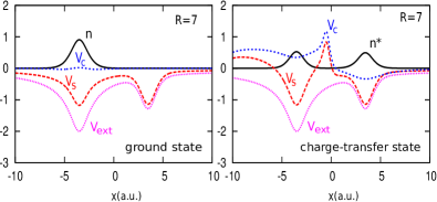
Figure 1: Density (black solid), $v_{\scriptscriptstyle\rm S}$ (red long-dashed), $v_{\scriptscriptstyle\rm C}$ (blue dashed), and $v_{\rm ext}$ (pink dotted) for the ground-state (left) and for the CT state (right) in our model molecule of closed-shell fragments at separation $R=7$au.

In Fig. 1, we show the density and the exact KS and correlation potentials for the ground and CT states for $R=7$au. A clear step and peak structure has developed in the correlation potential in the region of low-density between the ions in the CT state. There is no such structure in the initial potential of the ground-state. As the separation increases, the step in $v_{\scriptscriptstyle\rm C}$ saturates to a size

$$\Delta=|I_{D}^{N_{D}-1}-I_{A}^{N_{A}+1}|\;,$$ (5)

where $I_{D}^{N_{D}-1}=I_{D}^{N=1}$ is the ionization energy of the donor containing one electron, $I_{A}^{N_{A}+1}=I_{A}^{N=1}$ is that of the one-electron acceptor ion, and the result is written for a general $N_{D}(N_{A})$-electron donor(acceptor). Eq. (5) can be shown by considering the asymptotics of the donor and acceptor orbitals, adapting the argument made for the case of the ground-state of a molecule made of open-shell fragments HTR09 ; TMM09 . Here instead, we have a step in the potential of a CT excited-state of a molecule made of closed-shell fragments.

Somewhat of the reverse picture occurs for the case of CT between open-shells: the initial ground-state correlation potential contains a step and peak, as shown earlier in P85b ; AB85 ; GB96 ; TMM09 ; HTR09 , that disappears as the CT state is reached. In either case, the step is a signature of of the strong correlation due to the delocalization of the KS orbital.

The step requires a spatially non-local density-dependence in the correlation functional, as in the ground-state case P85b ; AB85 ; GB96 ; TMM09 ; HTR09 . The inability of usual ground-state approximate functionals to capture this step results in them incorrectly predicting fractionally charged species. In the present case, we have an excited state of the interacting system, where the KS orbital corresponding to the excited-state density $n^{*}$ shown in Fig. 1 is in fact a ground-state orbital, $\phi(x)=\sqrt{n^{*}(x)/2}$, because $n^{*}$ has no nodes. Given the static ground-state nature of the orbital and KS potentials after time $T$, does the adiabatic approximation become exact?

To answer this, we examine the adiabatically-exact xc potential for $t>T$, $v_{\scriptscriptstyle\rm XC}^{adia-ex}[n^{*}]$, i.e. evaluating the exact ground-state xc functional on the instantaneous CT density. This is (see Refs. TGK08 ; EM12 ):

$$v_{\scriptscriptstyle\rm XC}^{adia-ex}[n]=v_{\scriptscriptstyle\rm S}^{adia}[n]-v_{\rm ext}^{adia}[n]-v_{\scriptscriptstyle\rm H}[n]$$ (6)

where $v_{\rm ext}^{adia}[n]$($v_{\scriptscriptstyle\rm S}^{adia}[n]$ ) is the external(exact ground-state KS) potential for two interacting electrons in a ground-state of this density ($v_{\scriptscriptstyle\rm S}^{adia}[n]$ corresponds to first two terms of Eq. (3)). Fig. 2 shows $v_{\scriptscriptstyle\rm C}^{adia-ex}[n^{*}]$ for two separations $R=7$au and 10au (see Supporting Information for numerical methods). Evidently, the adiabatic approximation does yield a step, but of the wrong size.

To understand this, first consider the functional dependence of the exact xc potential. We may write (MBW02 )

$$v_{\scriptscriptstyle\rm XC}[n](t>T)=v_{\scriptscriptstyle\rm XC}[n^{*},\Psi^{*},\Phi_{CT}^{gs}](t>T)\;,$$ (7)

where, on the left, the dependence is on the entire history of the density, $n(0<t<T)$, and initial-state dependence is not needed since at $t=0$ we start from the ground-state newTDDFTbook ; MBW02 . On the right, time $T$ is considered as the “initial” time, and the functional depends on just the static density $n^{*}$ after this time, but, crucially, the interacting state and KS states at time $T$. The former is the CT excited state $\Psi^{*}$, while the latter is the doubly-occupied orbital: $\Phi(x_{1},x_{2},T)=\sqrt{n^{*}(x_{1})n^{*}(x_{2})}/2\equiv\Phi_{CT}^{gs}$, a ground-state wavefunction, as discussed above.

On the other hand, the adiabatic approximation

$$v_{\scriptscriptstyle\rm XC}^{adia}[n^{*}]\equiv v_{\scriptscriptstyle\rm XC}^{adia}[n^{*},\Psi_{CT}^{gs},\Phi_{CT}^{gs}]\;,$$ (8)

differs from the exact xc potential Eq. (7), in its dependence on the time-$T$ interacting state: here $\Psi_{CT}^{gs}$ is the ground-state wavefunction of an interacting system with density $n^{*}$, not the true excited state wavefunction. Therefore, Eqs. (7) and (8) show that the adiabatically-exact xc potential is not the same as the exact xc potential: the initial-state dependence in the exact functional reflects a nonlocal time-dependence that persists forever. In the infinite-separation limit, we expect $\Psi^{*}$ and $\Psi_{CT}^{gs}$ to be very similar, both having a Heitler-London form with one electron in each well, but the fact that $\Psi^{*}$ is an excited state is encoded in the nodal structure of its wavefunction. The correlation potential is extremely sensitive to this tiny difference in the two interacting wavefunctions, which accounts for the different step size in Fig. 2.

The magnitude of the step in $v_{\scriptscriptstyle\rm XC}^{adia-ex}$ in the infinite-separation limit can be derived by examining the terms in Eq. (6). In this limit, locally around each well $v_{\rm ext}^{adia}$ must equal the atomic potential, up to a spatial constant, in order for $\Psi_{CT}^{gs}[n^{*}]$ to satisfy Schrödinger’s equation there. It cannot simply be the sum of the atomic potentials, because the ground-state $\Psi_{0}$ of that potential (Eq. 2) places two electrons in the donor well. For $\Psi_{CT}^{gs}$ to be the ground state, $v_{\rm ext}^{adia}$ has a step in the region of negligible density that pushes up the donor well relative to the acceptor well; the size of this step, $C$, is the lowest such that energetically it is favorable to place one electron on each well, as $\Psi_{CT}^{gs}[n^{*}]$ does. So,

$$E^{gs,N=1}_{D}+E_{A}^{gs,N=1}+C<E^{gs,N=2}_{D}+2C$$ (9)

where $E^{gs,N}_{D(A)}$ is the ground-state energy of the N-electron donor(acceptor). This leads to

$$C \geq E^{gs,N=1}_{D}+E_{A}^{gs,N=1}-E^{gs,N=2}_{D}=I_{D}^{N_{D}}-I_{A}^{N_{A}+1}$$ (10)

where in the last line, we have generalized the result to a donor(acceptor) with $N_{D}(N_{A})$ electrons.

Now that we have the step in $v_{\rm ext}^{adia}[n^{*}]$, we use Eq. (6) to quantify the step in $v_{\scriptscriptstyle\rm XC}^{adia-ex}[n^{*}]$. Since $v_{\scriptscriptstyle\rm S}^{adia}=v_{\scriptscriptstyle\rm S}^{\rm exact}$ here, Eq. 5 tells us that the step in $v_{\scriptscriptstyle\rm C}^{adia-ex}$ is

$$\Delta_{adia}=|I_{D}^{N_{D}-1}-A_{D}^{N_{D}-1}|$$ (11)

which is equal to the derivative discontinuity of the $(N_{D}-1)$-electron donor. (As before, the entire step is contained in the correlation potential). For our system $I_{D}^{N=1}=1.483$au, $A_{D}^{N=1}=0.755$au and $I_{A}^{N=1}=0.5$au, thus in the infinite separation limit we get a step of $0.983(0.729)$au in the exact $v_{\scriptscriptstyle\rm C}$($v_{\scriptscriptstyle\rm C}^{adia}$). The numerical results verify this analysis; the steps shown in Figure 2 for separation $R=7$($R=10$)au have values of $0.61$ (0.76)au in the exact $v_{\scriptscriptstyle\rm C}$ and $0.42$ (0.55)au in $v_{\scriptscriptstyle\rm C}^{adia}$. For larger separations, the steps tend towards the asymptotic values predicted by the analysis above.

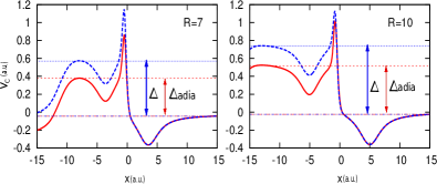
Figure 2: The exact $v_{\scriptscriptstyle\rm C}$ (dashed blue line) and the adiabatically-exact $v_{\scriptscriptstyle\rm C}^{adia-ex}$ (red solid line) for $R=7$au (left) and for $R=10$ au(right). Note that the potential eventually rolls back down to zero far enough away from the system. In the infinite separation limit $\Delta$($\Delta_{adia}$)is given by Eq. (5)(Eq. (11)).

In the above analysis, the adiabatically-exact potential was evaluated on the exact density, as is commonly done when assessing functionals TGK08 , rather than on that obtained from a self-consistent adiabatic propagation. The latter would likely lead to an erroneous density at time $T$, but the analysis shows that even with the exact density at time $T$, the wrong step-size means that subsequent propagation using the adiabatically-exact potential will yield the wrong dynamics.

Having studied how the xc potential looks for the final CT state, we now study how the potential evolves in time to reach such a state. To simplify the analysis we exploit Rabi physics to reduce this problem to a two-state system. This approach is justified for weak resonant driving field, and verified numerically by comparing the results with the exact time-dependent wavefunction found using octopus octopus ; octopus2 ; octopus3 . The interacting wavefunction may be written as $|\Psi(t)\rangle=a_{g}(t)|\Psi^{gs}\rangle+a_{e}(t)|\Psi^{*}\rangle$, where

$$i\partial_{t}\left({\begin{array}[]{c}a_{g}(t)\\ a_{e}(t)\\ \end{array}}\right)=\left({\begin{array}[]{cc}E_{g}-d_{gg}{\cal E}(t)&-d_{eg}{\cal E}(t)\\ -d_{eg}{\cal E}(t)&E_{e}-d_{ee}{\cal E}(t)\\ \end{array}}\right)\left({\begin{array}[]{c}a_{g}(t)\\ a_{e}(t)\end{array}}\right)$$ (12)

with $d_{eg}=d_{ge}=0.231$, $d_{gg}=7$ and $d_{ee}=0$ for our system. The electric field is resonant with the first excitation: ${\cal E}(t)=0.006\cos(0.112t)$.

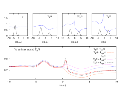
Figure 3: Upper panel: The correlation potential (dotted blue line) and density (solid black) shown at snapshots of time indicated. Lower panel: Vc at snapshots over an optical cycle centered around $T_{R}/8$.

Fig. 3 displays the correlation potential at snapshots in time over a half-Rabi period $T_{R}/2$ fnote2 . The step, accompanied by a peak, develops over time as the excited CT state is reached; at $T_{R}/2$ the correlation potential agrees with the static prediction earlier (Fig. 2, left). Notice that making a time-dependent constant shift does not affect the dynamics, just adds a time-dependent overall phase. During the second half of the Rabi cycle, the step gradually disappears. A closer inspection indicates that superimposed to this smoothly developing step, is an oscillatory step structure, whose dynamics is more on the time-scale of the optical field (lower panel). This faster, non-adiabatic, non-local dynamical step appears generically in electron dynamics, as shown in Ref. EFRM12 . To distinguish between the two steps we refer to the more gradually developing step due to CT, as the “CT step”.

The impact that the development of the CT step has on dynamics is significant. The same adiabatic approximations that for local resonant excitations showed faster but still Rabi-like oscillations FHTR11 , fail dramatically to capture any Rabi-like oscillations between the ground and CT state. This is illustrated by the dipole moments, $d(t)=\langle\psi(t)|\hat{x}_{1}+\hat{x}_{2}|\psi(t)\rangle$, in Figure (4). The approximate correlation functionals lack the non-local spatial-dependence necessary to develop the CT step (fnote3 ).

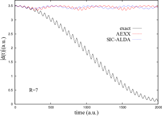
Figure 4: Absolute value dipole moments $|d(t)|$ for the CT between closed-shell fragments at separation $R=7$au for exact (solid black line), adiabatic exact-exchange (AEXX) (dashed red line) and self-interaction-corrected adiabatic local density approximation (SIC-ALDA)(dotted blue line). The calculations were performed in the presence of a resonant field of frequency $\omega=0.112$ and amplitude $A=0.00667$.

Given the ubiquity of CT dynamics in topical applications of TDDFT, it is critical to develop approximations with spatially non-local and non-adiabatic dependence. None of the available functionals today captures the peak and step structure that develop in the exact $v_{\scriptscriptstyle\rm C}$ as the charge transfers, and they lead to drastically incorrect dynamics, as illustrated in Figure 4. Even an exact adiabatic approximation will be incorrect: a step and peak feature are captured but of the wrong size. The performance of a self-consistent propagation in such a potential is left for a future investigation, as is the role of the peak that accompanies the step. Superimposed on the development of the CT step, are the generic dynamical step and peak features of Ref EFRM12 : this features depends on the details of how the CT is induced, e.g. oscillating on the time-scale of a resonant optical field. Note that the CT step recedes asymptotically far from the molecule HTR09 ; TMM09 , while the dynamical step persists EFRM12 . The relation of these structures to the derivative discontinuities of the xc kernel for CT excitations HG12 will also be investigated in the future.

In modeling real systems the vibronic coupling introduces a mixture of excited states that are not, in principle, fully populated. Still our findings apply, since for an ensemble of states CT steps and dynamical steps appear that account for the population of each excited state contributing to the wave packet. Note that the step responsible for the CT appears as soon as the state starts to be populated. Recent work has shown that TDDFT describes the CT process in an organic photovoltaic Rozzi ; our findings may explain the observed incomplete CT of the electron to the fullerene Rozziprivate . The step feature is a fundamental one for describing processes where electron-hole splitting is key. Our work highlights an essential new feature that must be considered in the development of nonadiabatic functionals able to capture dynamical electron transfer processes.

Acknowledgments We gratefully acknowledge financial support from the US Department of Energy, Office of Basic Energy Sciences, Division of Chemical Sciences, Geosciences and Biosciences and Award DE-SC0008623 (NTM), and a grant of computer time from the CUNY High Performance Computing Center under NSF Grants CNS-0855217. The European Research Council (ERC-2010- AdG -267374) , Spanish: FIS2011- 65702- C02-01), Grupos Consolidados (IT-319-07), and EC project CRONOS (280879-2) and CNS- 0958379, are gratefully acknowledged. JIF acknowledges support from an FPI fellowship (FIS2007-65702- C02-01).

Supporting Information Available: All numerical aspects of the calculations are contained in the Supporting Information. This information is available free of charge via the Internet at http://pubs.acs.org/.

References

- (1) Runge, E.; Gross, E.K.U. Density-Functional Theory for Time-Dependent Systems. Phys. Rev. Lett. 1984, 52, 997-1000.
- (2) Fundamentals of Time-Dependent Density Functional Theory, (Lecture Notes in Physics 837), eds. Marques, M.A. L.; Maitra, N.T.; Nogueira, F.; Gross, E.K.U.; Rubio, A. (Springer-Verlag, Berlin, Heidelberg, 2012).
- (3) Themed Issue on Time-Dependent Density Functional Theory. Phys. Chem. Chem. Phys 2009, 11, eds. Marques, M. A. L.; Rubio, A.
- (4) Autschbach, J., Charge-Transfer Excitations and Time-Dependent Density Functional Theory: Problems and Some Proposed Solutions. ChemPhysChem 2009, 10, 1757-1760, and references therein.
- (5) Stein, T.; Kronik, L.; Baer, R. Reliable Prediction of Charge Transfer Excitations in Molecular Complexes Using Time-Dependent Density Functional Theory. J. Am. Chem. Soc. 2009, 131, 2818–2821.
- (6) Baer, R.; Livshits, E.; Salzner, U. Tuned Range-Separated Hybrids in Density Functional Theory. Annu. Rev. Phys. Chem. 2010, 61, 85–109.
- (7) Hellgren, M.; Gross, E. K. U., Discontinuities of the Exchange-Correlation Kernel and Charge-Transfer Excitations in Time-Dependent Density-Functional Theory. Phys. Rev. A. 2012, 85, 022514-1–6.
- (8) Maitra, N. T. Undoing Static Correlation: Long-Range Charge Transfer in Time-Dependent Density-Functional Theory, J. Chem. Phys. 2005, 122, 234104-1–6.
- (9) Maitra, N. T.; Tempel, D. G. Long-Range Excitations in Time-Dependent Density-Functional Theory. J. Chem. Phys. 2006, 125, 184111-1–6.
- (10) Fuks, J. I.; Rubio, A.; Maitra, N.T. Charge Transfer in Time-Dependent Density-Functional Theory via Spin-Symmetry Breaking, Phys. Rev. A. 2011, 83, 042501-1–5.
- (11) Tempel, D. G.; Maitra, N. T.; Martinez, T. J. Revisiting Molecular Dissociation in Density Functional Theory: A Simple Model. J. Chem. Theory Comput. 2009, 5, 770–780.
- (12) Helbig, N.; Tokatly, I. V.; Rubio, A. Exact Kohn-Sham Potential of Strongly Correlated Finite Systems. J. Chem. Phys. 2009, 131, 224105-1–8.
- (13) Prezhdo, O. V.; W. R. Duncan, W. R.; and Prezhdo, V. V. Photoinduced Electron Dynamics at the Chromophore-Semiconductor Interface: A Time-Domain Ab Initio Perspective. Prog. Surf. Sci. 2009, 84, 30–68.
- (14) Oviedo, M.; Zarate, X.; Negre, C. F. A.; Schott, E.; Arriatia-Pérez R.; Sánchez, C. G. Quantum Dynamical Simulations as a Tool for Predicting Photoinjection Mechanisms in Dye-Sensitized Ti02 Solar Cells. J. Phys. Chem. Lett. 2012, 3, 2548–2555.
- (15) Teoh, W. Y.; Scott, J. A.; Amal, R. Progress in Heterogeneous Photocatalysis: From Classical Radical Chemistry to Engineering Nanomaterials and Solar Reactors. J. Phys. Chem. Lett. 2012, 3, 629–639.
- (16) Nguyen, P. et al. Solvated First-Principles Excited-State Charge-Transfer Dynamics with Time-Dependent Polarizable Continuum Model and Solvent Dielectric Relaxation. J. Phys. Chem. Lett. 2012, 3, 2898–2904.
- (17) Moore, J.E.; Morton, S.M.; Jensen, L. Importance of Correctly Describing Charge-Transfer Excitations for Understanding the Chemical Effect in SERS. J. Phys. Chem. Lett. 2012, 3, 2470–2475
- (18) Meng, S.; Kaxiras,E. Electron and Hole Dynamics in Dye-Sensitized Solar Cells: Influencing Factors and Systematic Trends. Nano Lett. 2010, 10, 1238–1247.
- (19) Some degree of spatial and time non-locality is introduced in orbital functionals, such as hybrid functionals that mix in a fraction of non-local exchange KK09 ; BLS10 .
- (20) Kümmel, S.; Kronik, L. Orbital-Dependent Density Functionals: Theory and Applications. Rev. Mod. Phys. 2008, 80, 3–60.
- (21) Elliot, P.; Fuks, J. I.; Maitra, N.T.; Rubio, A. Universal Dynamical Steps in the Exact Time-Dependent Exchange-Correlation Potential. Phys. Rev. Lett. 2012, 109, 266404-1–5.
- (22) Javanainen, J.; Eberly, J.; Su, Q. Numerical simulations of multiphoton ionization and above-threshold electron spectra. Phys. Rev. A. 1988, 38, 3430–3446.
- (23) Lappas, D.G.; Sanpera, A.; Watson, J.B.; Burnett, K.; Knight, P.L; Grobe, R.; Eberly, J.H. Two-electron effects in harmonic generation and ionization from a model He atom. J. Phys. B, 1996, 29, L619 , 16
- (24) Villeneuve, D.M.; Ivanov, M.Y.;Corkum, P.B. Enhanced ionization of diatomic molecules in strong laser fields: A classical model. Phys.Rev. A. 1996, 54, 736–741
- (25) Bandrauk, A.; Ngyuen, H. Attosecond control of ionization and high-order harmonic generation in molecules. Phys. Rev. A. 2002, 66, 031401
- (26) Bandrauk, A.D.; Lu, H. Laser-induced electron recollision in H2 and electron correlation. Phys. Rev. A2005,72, 023408
- (27) Kreibich , T. et al.. Even-Harmonic Generation due to Beyond-Born-Oppenheimer Dynamics. Phys. Rev. Lett. 2001,87, 103901
- (28) Kreibich, T.; van Leeuwen, R.; Gross, E. K. U.. Time-dependent variational approach to molecules in strong laser fields. Chem. Phys.2004, 304, 183-202.
- (29) Perdew, J. P. in Density Functional Methods in Physics, edited by Dreizler R.M. and da Providencia, J.; Plenum: New York, 1985.
- (30) Almbladh, C. O. ;von Barth, U. in Density Functional Methods in Physics, edited by Dreizler, R.M. and da Providencia, J.; Plenum: New York, 1985.
- (31) Gritsenko, O.V.; Baerends, E.J. Effect of Molecular Dissociation on the Exchange-Correlation Kohn-Sham Potential. Phys. Rev. A 1996, 54, 1957 –1972.
- (32) Castro, A. et al.. Octopus: A Tool for the Application of Time-Dependent Density Functional Theory. Phys. Stat. Sol. (b) 2006, 243, 2465–2488.
- (33) Marques, M. A. L.; Castro, A.; Bertsch, G. F.; Rubio, A. Octopus: A First-Principles Tool for Excited Electron-Ion Dynamics. Comp. Phys. Comm. 2003, 151, 60–78.
- (34) Andrade, X. et al. Time-Dependent Density-Functional Theory in Massively Parallel Computer Architectures: The Octopus Project. J. Phys.: Condens. Matter 2012, 24 233202–1–11.
- (35) Thiele, M.; Gross, E.K.U.; Kümmel, S. Adiabatic Approximation in Nonperturbative Time-Dependent Density-Functional Theory. Phys. Rev. Lett. 2008, 100, 153004-1–4.
- (36) Elliott, P.; Maitra, N. T. Propagation of Initially Excited States in Time-Dependent Density Functional Theory. Phys. Rev. A. 2012, 85, 052510-1–11.
- (37) Maitra, N.T.; Burke, K.; Woodward, C. Memory in time-dependent density functional theory. Phys. Rev. Lett. 2002, 89, 023002-1–4.
- (38) Within the rotating wave approximation , where is a Bessel function with argument (see Ref. BMT00 for details). The CT state for our model is reached at .
- (39) Fuks, J. I.; Helbig, N.; Tokatly, I.V.; Rubio, A. Nonlinear phenomena in time-dependent density-functional theory: What Rabi oscillations can teach us. Phys. Rev. B. 2011, 84, 075107.
- (40) For smaller separations the approximations perform better, as their character becomes more local; but errors remain without non-adiabatic non-local dependence needed in the potential EFRM12 .
- (41) Brown, A.; Meath, W.J.; Tran, P. Rotating-Wave Approximation for the Interaction of a Pulsed Laser with a Two-Level System Possessing Permanent Dipole Moments. Phys Rev. A. 2000, 63, 013403-1–7. .
- (42) Rozzi, C.A. et al. Quantum Coherence Controls the Charge Separation in a Prototypical Artificial Light Harvesting System. Nature Communications 2013, in press.
- (43) Rozzi, C.A.; Rubio, A. private communication.