On the (non-)enhancement of the Ly$\alpha$ equivalent width
by a multiphase interstellar medium

Abstract

It has been suggested that radiative transfer effects may explain the unusually high equivalent widths (EWs) of the Ly$\alpha$ line, observed occasionally from starburst galaxies, especially at high redshifts. If the dust is locked up inside high-density clouds dispersed in an empty intercloud medium, the Ly$\alpha$ photons could scatter off of the surfaces of the clouds, effectively having their journey confined to the dustless medium. The continuum radiation, on the other hand, does not scatter, and would thus be subject to absorption inside the clouds.

This scenario is routinely invoked when Ly$\alpha$ EWs higher than what is expected theoretically are observed, although the ideal conditions under which the results are derived usually are not considered. Here we systematically examine the relevant physical parameters in this idealized framework, testing whether any astrophysically realistic scenarios may lead to such an effect. It is found that although clumpiness indeed facilitates the escape of Ly$\alpha$, it is highly unlikely that any real interstellar media should result in a preferential escape of Ly$\alpha$ over continuum radiation. Other possible causes are discussed, and it is concluded that the observed high EWs are more likely to be caused by cooling radiation from cold accretion and/or anisotropic escape of the Ly$\alpha$ radiation.

1. Introduction

Our understanding of the high-redshift Universe has expanded tremendously during the last decade, especially due a single specific emission line, the Ly$\alpha$ line. Tracing in particular galaxies in the process of forming, the shape, intensity, and spatial distribution of this line carry a wealth of information. However, while our theoretical understanding of the physical processes that govern the radiative transfer (RT) of Ly$\alpha$ has also advanced significantly, it is evident that the complexity of density fields, gas kinematics, dust distribution, line formation, impact of the intergalactic medium (IGM), etc. render individually observed lines quite difficult to interpret in detail.

As Ly$\alpha$ emitting galaxies (LAEs) generally are relatively small (Gawiser et al., 2006; Lai et al., 2007; Nilsson et al., 2007) of low (specific) star formation rate (Fynbo et al., 2003; Nilsson et al., 2010), our lack of knowledge is in part due to the difficulties in observing faint galaxies. This obstacle may to some extend be overcome using gravitationally lensed LAEs (e.g. Fosbury et al., 2003; Quider et al., 2009; Christensen et al., 2012a, b), which may boost the observed flux by more than an order of magnitude. Larger surveys of the statistical properties of LAEs, such as their luminosity function (LF, Ouchi et al., 2005, 2008; Shimasaku et al., 2006; Kashikawa et al., 2006; Dawson et al., 2007; Grove et al., 2009) and clustering properties (Gawiser et al., 2007; Gronwall et al., 2007) may overcome some of these complications, although still our ignorance of RT processes easily may result in systematic errors. A common technique by which to assess the stellar population of individual galaxies at high redshifts is to measure the equivalent width (EW) $W$ of the Ly$\alpha$ line (e.g. Gronwall et al., 2007; Ouchi et al., 2008; Stark et al., 2010). This quantity is defined as the ratio of the integrated line flux to continuum flux density, $W=\int\!d\lambda\,[F(\lambda)\!-\!F_{0}]/\!F_{0}$, where the exact limits of the integral are not important, as long as the full line is included. For sloped continua, the wavelength dependency of the continuum must also be taken into account. For high EWs, $W$ can be approximated by the relative escape fraction of Ly$\alpha$ and continuum photons. The EW depends on galactic parameters such as the initial mass function (IMF) and the gas metallicity (e.g. Schaerer, 2002), and can consequently be used as a probe of these quantities.

In young galaxies, Ly$\alpha$ is produced mainly from recombinations following the ionization of hydrogen surrounding O and B stars. Since these stars are short-lived, a few Myr after an initial starburst the EW will generally decrease significantly. Stellar population syntheses (e.g. Charlot & Fall, 1993; Valls-Gabaud, 1993; Schaerer, 2003) predict that the EW should initially reach $\sim 240$ Å, eventually declining and settling on roughly 80 Å, where the exact values depend on the assumed IMF and metallicity of the population. Curiously, several observational studies have reported on the detection of much higher EWs (e.g. Hu & McMahon, 1996; Kudritzki et al., 2000; Malhotra & Rhoads, 2002; Rhoads et al., 2003; Dawson et al., 2004; Hu et al., 2004; Shimasaku et al., 2006; Gronwall et al., 2007; Ouchi et al., 2008; Nilsson et al., 2009; Kashikawa et al., 2011, 2012). While some of these extreme EW galaxies can be attributed to AGN activity, in many cases this explanation is explicitly excluded. Moreover, such high EWs are not readily explained by simply assuming a more top-heavy IMF. Indeed, the observations pose a serious challenge to our understanding of both galaxy formation, stellar evolution, and radiative transfer.

In this work, we will distinguish between three related notations. The equivalent width $W_{\mathrm{int}}$ of the intrinsically emitted spectrum is given by the stellar population; for instance, a more top-heavy IMF emits a harder spectrum, with relatively more ionizing and hence Ly$\alpha$ photons. When escaping the galaxy, the spectrum has an equivalent width $W_{\mathrm{em}}$; as we shall see below, the ISM may possess the ability of transferring an uneven fraction of Ly$\alpha$ vs. continuum photons, making $W_{\mathrm{em}}$ larger or smaller than $W_{\mathrm{int}}$. Finally, as the total number of photons in a line is conserved when traveling through the Universe, whereas the number of continuum photons per wavelength bin is reduced as they are cosmologically redshifted, the observed equivalent width $W_{\mathrm{obs}}$ from a source at redshift $z$ is given by $W_{\mathrm{obs}}=(1+z)W_{\mathrm{em}}$.

1.1. The Neufeld scenario

As Ly$\alpha$ photons scatter on neutral hydrogen, their path length before escaping a galaxy will always be longer than that of continuum radiation. Thus, the immediate corollary is that Ly$\alpha$ will be more susceptible to dust absorption than the continuum, implying that $W_{\mathrm{em}}<W_{\mathrm{int}}$. However, Neufeld (1991, hereafter N91) investigated analytically the resonant scattering of Ly$\alpha$ photons through the ISM and found that under special circumstances, the Ly$\alpha$ photon may actually suffer less attenuation than radiation which is not resonantly scattered, e.g. continuum radiation. N91 considered the escape of radiation from the center of a plane-parallel, two-phase structure, in which sperical clouds of homogeneously mixed neutral hydrogen and dust lie embedded within a virtually empty intercloud medium (ICM). The number density of clouds are assumed to be small enough that they do not touch, yet sufficiently numerous that they cover most of the sky.

Furthermore, the source of both Ly$\alpha$ and continuum photons is assumed to be pointlike and situated in the center of the slab, in the ICM. Under these conditions N91 showed that Ly$\alpha$ photons, upon entering a cloud, scatters only a few times before returning to the ICM, thereby being exposed arbitrarily little to absorption by dust. Consequently, the journey of the Ly$\alpha$ photons will be confined primarily to the dustless ICM, preserving the total Ly$\alpha$ luminosity. In contrast, the continuum radiation which penetrates the clouds rather than scattering off of their surfaces will be subject to the full attenuation, given by the optical depth of dust from the center and out.

Thus, since the continuum is reduced while the line is more or less preserved, the EW of the escaping radiation can be “boosted” to arbitrarily high values. We define such a boost as

$$b\equiv\frac{W_{\mathrm{em}}}{W_{\mathrm{int}}}.$$ (1)

Of course, the boost does not imply an increased Ly$\alpha$ luminosity, but rather a reduced continuum luminosity.

1.2. Numerical and observational support

The mere potential of an EW boost was the conclusion of N91’s studies. Hansen & Oh (2006, hereafter HO06) studied the scenario in more detail, both analytically and numerically. In addition to confirming the boost, they also looked into the effect of galactic outflows of clumpy gas on the line profile, exploring the RT in various geometries.

While HO06 did investigate various extensions of the Neufeld scenario, one of their main conclusion was the same as N91: “If most of the dust resides in a neutral phase which is optically thick to Ly$\alpha$, the Ly$\alpha$ EW can be strongly enhanced”. The results of N91 and HO06 seem a natural explanation of the unusually high observed EWs, and lately such observations has routinely been interpreted within the framework of this scenario, inferring the presence, or non-presence, of a clumpy, dusty ISM. Thus, Chapman et al. (2005) and lately Bridge et al. (2012), interpret the fact that Ly$\alpha$ radiation is visible from $\sim 50$% of a sample of sub-mm galaxies as suggesting the presence of very patchy and inhomogeneous dust distribution. Finkelstein et al. (2007) regards a clumpy ISM as a possible explanation of their high Ly$\alpha$ EWs, and in Finkelstein et al. (2008) propose a parameter $q$ to characterize clumpiness, such that Ly$\alpha$ is attenuated by a factor $e^{-q\tau}$, where $\tau$ is the dust optical depth for non-resonant photons close to the Ly$\alpha$ line. For a given Ly$\alpha$ EW observation they then calculate the clumpiness of the ISM, positing that for $q<1$ the EW is boosted due to dust clumpiness. This method is further used in Finkelstein et al. (2009a, c, 2011a), Yuma et al. (2010), Blanc et al. (2011), Nakajima et al. (2012) and Hashimoto et al. (2012) to infer various degrees of clumpiness in observed LAEs. A equivalent approach was followed in Niino et al. (2009) and Kobayashi et al. (2010). Similarly, Dayal et al. (2008, 2009, 2010, 2011) has invoked a clumpy ISM scenario in order to match their simulated LAE LFs to observed ones.

However, the idealized conditions under which a boost may be achieved is rarely taken into account. Accordingly, we believe that a revision of the scenario is timely, and in the present work we aim to investigate the validity of the various premises of the model. We do this by calculating numerically the RT of Ly$\alpha$ and continuum in model galaxies constructed to cover a broad range of plausible as well as implausible systems. In addition to the work of N91 and HO06, the topic of resonant scattering in a multiphase medium has received attention from Richling et al. (2003), Šurlan et al. (2012), Dijkstra & Kramer (2012), and Duval et al. (2012). Of these, only Duval et al. (2012) concern themselves with the relative escape fraction of Ly$\alpha$ and continuum, and found tentative evidence for the impracticability of enhancing the Ly$\alpha$ EW, by investigating the Ly$\alpha$ and continuum RT in an expanding shell of clumps with different values of dust optical depth, expansion velocity, Hi density, and line width. They found that indeed a virtually empty ICM was needed, along with only modest outflow velocities and high $E(B-V)$, for an ISM geometry to result in a boost.

After describing the principles of the applied numerical code in Sec. 2, we systematically vary all parameters relevant for decribing a (model) galaxy in Sec. 3, one at a time. This gives us a feeling for the impact a given parameter has on the boost. However, as the change of one parameter may very well be either enhanced or counteracted by the change of another, after discussing in Sec. 4 observational and theoretical constraints on the actual values of the parameters that are likely to be met in real astrophysical situations, we subsequently, in Sec. 5, undertake a large sample of simulations with random parameters covering these values, constructing a likelihood map of achievable boosts. The results of these calculations are discussed in Sec. 6, along with a discussion on other possible scenarios that could lead to high Ly$\alpha$ EWs.

2. Radiative transfer simulations

N91 regarded each dusty cloud as a scattering particle itself, with a certain probability of absorbing a photon. When HO06 developed their numerical model, they followed the same approach. They used a Monte Carlo code, where the path of individual photons were traced as they traveled through the ICM, but whenever a cloud was encountered, the photon would simply be absorbed or scattered at once in some direction away from the cloud. The appropriate probability density functions (PDFs) were calculated on beforehand from fits to a series of RT calculations of photons incident on a cloud surface. This rendered feasible simulations that were otherwise impractical. In the almost seven years that have passed since, computational power has increased to a point that “brute force” simulations can in fact be performed rather effortlessly, obliviating the need for several approximations.

In the present work, the RT calculations are conducted using the numerical code MoCaLaTA (Laursen et al., 2009a, b). In the following, the basics of the code are outlined:

The galaxy is constructed on a grid of cells, each of which holds a value of the physical parameters important to the RT; the neutral hydrogen density $n_{\textrm{{\scriptsize H}{\tiny\hskip 0.28453ptI}}}$, the dust density $n_{\textrm{d}}$, the gas temperature $T$, and the three-dimensional velocity $\mathbf{v}_{\mathrm{bulk}}$ of the gas elements. The original Neufeld scenario concerned itself with radiation escaping from a slab of gas. For numerical reasons, higher resolution can be achieved considering radiation escaping a sphere of multiphase gas, as did also HO06. Qualitatively, and even quantitatively except for factors of order unity, the results are equivalent. Thus, a galaxy is modeled as a number $N_{\mathrm{cl}}$ of spherical, non-overlapping clouds with radius $r_{\mathrm{cl}}$, dispersed randomly within a sphere of radius $r_{\mathrm{gal}}$. A cell may be either an ICM cell or a cloud cell. In order to make the clouds spherical, cells on the border between a cloud and the ICM are adaptively refined, such that a given cell is split into eight subcells, recursively until a satisfactory resolution is achieved. The structure is depicted in LABEL:AMR, where also a surface brightness map of a simulation is shown.

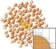
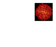
Figure 1.— Left: Graphical representation of the design of the model galaxy with $\sim 200$ clouds. The AMR structure with six levels of refinement is illustrated in the inset. Note that for presentation purposes only, a two-dimensional analogy is shown; in reality all simulations are carried out in three dimensions. Right: Simulated surface brightness map of a model with $\sim 500$ rather large clouds of radius $r_{\mathrm{cl}}=350$ pc to emphasize the structure. The fiducial model used in Sec. 3 has 6500 clouds of $r_{\mathrm{cl}}=100$ pc, with a maximum refinement level of $\simeq 10$.

We typically consider $\sim 10^{3\textrm{-}5}$ clouds, with each cloud typically consisting of $10^{2\textrm{-}3}$ cells. Note however that the actual shape of a cloud does not affect the results significantly; the most important quantities, as identified by HO06, are the cloud albedo, i.e. the probability that a photon incident on a cloud is reflected rather than absorbed after a number of scatterings, and the average number $N_{0}$ of clouds with which a Ly$\alpha$ photon interacts before escaping the galaxy, in the absence of absorption. This number in turn is a function of the covering factor $f_{\mathrm{c}}$, which is the average number of clouds intercepted by a sightline from the center and out. Individual Ly$\alpha$ and continuum photons are then emitted and traced as they scatter in real and frequency space throughout the inhomogeneous ISM.

MoCaLaTA has previously been applied to galaxies extracted from cosmological simulations. Although it was tested thoroughly against various analytical solutions in Laursen et al. (2009a, b), some modifications and extensions had to be made in order to use it for the idealized simulations in the present study. These are described and tested in App. A.

For a given set of parameters $N_{\mathrm{cl}}$, $r_{\mathrm{cl}}$, etc., the observed boost will depend on the direction which it is observed, as well as on the actual random realization of cloud positions. In addition to sampling the average spectrum, i.e. the spectrum of photons escaping in all directions, MoCaLaTA calculates the spectra escaping exactly in the six different directions along the Cartesian axes. The more clouds a galaxy comprises, the smaller the spread will be in different directions, and for different realizations. Further, the variation between different directions is much larger than between different realizations. For instance, for a covering factor of $\mbox{$f_{\mathrm{c}}$}=2$, only $\sim 30$% of the sightlines will actually intercept two clouds, while $\sim 10$% will intercept no clouds at all (i.e. the covering fraction is $\sim 0.9$ for $\mbox{$f_{\mathrm{c}}$}\sim 2$), and a non-negligible fraction of the sightlines will intercept $\geq 5$ clouds. These three cases will, respectively, result in a boost close to the $4\pi$ average, no boost at all, and an essentially infinite boost (for a central point source). Thus, the fractional standard deviation $\sigma_{b}/b$ from different viewing angles is typically of order 50%, while for the $4\pi$ average of many realizations of the same model, $\sigma_{b}/b$ is but a few percent. In the following analysis, the presented values of $b$ represent the $4\pi$ average for a single realization of a given model.

3. Investigating the criteria for a boost

In order to systematize which physical conditions are necessary for boosting the EW, we first settle on a fiducial model. In the subsequent sections, several of the implied parameters are then relaxed or varied, individually or in conjunction. When nothing else is stated, the remaining parameters correspond to the fiducial model. Initially, we will not concern ourselves with the realism of the parameters, instead deferring this discussion to Sec. 4, although we note that several of the chosen values, as well as various derived parameters such as color excess and total galaxy mass, roughly resemble observed typical LAE values.

The fiducial model galaxy is a sphere of radius $r_{\mathrm{gal}}=5$ kpc consisting of $N_{\mathrm{cl}}=6500$ of clouds of equal radii $r_{\mathrm{cl}}=0.1$ kpc. The density of neutral hydrogen in the clouds is $n_{\textrm{{\scriptsize H}{\tiny\hskip 0.28453ptI}}}=1$ cm^-3, implying a column density $N_{\textrm{{\scriptsize H}{\tiny\hskip 0.28453ptI},cl}}\sim 3\times 10^{20}$ cm^-2 as measured from the center to the surface of a cloud. The clouds are dispersed at random in an empty ICM. The temperatures of the clouds and the ICM are $T_{\mathrm{cl}}=10^{4}$ and $T_{\mathrm{ICM}}=10^{6}$ K, respectively. The physical significance of the clouds and the ICM are the interstellar phases conventionally called the warm neutral medium (WNM) and the hot ionized medium (HIM), first identified by Field et al. (1969) and McKee & Ostriker (1977), although in reality $n_{\textrm{{\scriptsize H}{\tiny\hskip 0.28453ptI},cl}}$ is usually somewhat smaller than the chosen 1 atom cm^-3. Finally, in the fiducial model, all photons are emitted in the line center, from the ICM in the center of the sphere.

The covering factor $f_{\mathrm{c}}$ is analogous to an optical depth of clouds intercepted by a sightline from the center of the galaxy and out. With a number density $n_{\mathrm{cl}}=N_{\mathrm{cl}}/V_{\mathrm{gal}}$ of clouds, the covering factor of the fiducial model is then $\mbox{$f_{\mathrm{c}}$}=n_{\mathrm{cl}}r_{\mathrm{gal}}\sigma_{\mathrm{cl}}=\frac{3}{4}N_{\mathrm{cl}}(r_{\mathrm{cl}}/r_{\mathrm{gal}})^{2}\simeq 2$ (where $\sigma_{\mathrm{cl}}$ is the cross section of a cloud). Since an average sightline passing through a cloud traverses a distance $\langle d\rangle=V_{\mathrm{cl}}/\sigma_{\mathrm{cl}}=4r_{\mathrm{cl}}/3$ inside the cloud, the total path traveled inside clouds for an average sightline is $\langle d_{\mathrm{in\ clouds}}\rangle=\mbox{$f_{\mathrm{c}}$}\langle d\rangle=N_{\mathrm{cl}}r_{\mathrm{cl}}^{3}/r_{\mathrm{gal}}^{2}$.

At the heart of the EW boosting mechanism lies the assumption of the Ly$\alpha$ photons being shielded from the dust by neutral hydrogen while the non-scattered FUV continuum radiation is subject to the “full” dust absorption. Hence, the relevant quantity for dust absorption is the total average absorption optical depth $\langle\tau_{\mathrm{a}}\rangle$ of the dust throughout the galaxy. The dust absorption optical depth of a single cloud (center-to-face) is $\tau_{\mathrm{a,cl}}=(1-A)\tau_{\mathrm{d,cl}}$, where $\tau_{\mathrm{d,cl}}$ is the total (absorption + scattering) dust optical depth, and $A$ is the dust albedo. Hence, $\langle\tau_{\mathrm{a}}\rangle\simeq\tau_{\mathrm{a,cl}}\langle d_{\mathrm{in\ clouds}}\rangle/r_{\mathrm{cl}}$ (this expression is only approximate, since photons scattering on dust grains may still be subject to absorption by another dust grain before it escapes the galaxy).

Dust grains are built from metals, and the density of dust is thus assumed to scale with metallicity and hydrogen density. Since observationally the optical depth is not readily measured, we will instead refer to the metallicity $Z$, which is usually more easily probed. Depending on the actual extinction curve used, the constant of proportionality will differ. Furthermore, assuming that the density of dust scales linearly with the metallicity, the dust optical depth can be related to $Z$ through $\tau_{\mathrm{d}}=N_{\mathrm{H}}\,\sigma_{\mathrm{d}}(\lambda)\,Z/Z_{0}$, where $\sigma_{\mathrm{d}}$ is the dust cross section per hydrogen nucleus — specific for a given extinction curve — and $Z_{0}$ is the reference metallicity of that extinction curve. For example, for SMC dust, at the Ly$\alpha$ wavelength the cross section is $\sigma_{\mathrm{d}}=4\times 10^{-22}$ cm² with only a small wavelength depence across the line, and the SMC metallicity is $Z_{0}\simeq 0.25\mbox{$Z_{\odot}$}$.

Having explicated the basics of the model, we now proceed to investigate the impact on the boost of varying the implied parameters.

3.1. Cloud covering factor

For the Neufeld scenario to be efficient, the sky, as seen from the center of the galaxy, must be sufficiently covered by clouds. N91 asserts that the covering factor $f_{\mathrm{c}}$ must be larger than unity. In fact, as soon as a single cloud is present, the $4\pi$ average will have $b>1$. Figure 2 shows, for various values of $n_{\textrm{{\scriptsize H}{\tiny\hskip 0.28453ptI},cl}}$ and $Z$ how the EW boost changes with $f_{\mathrm{c}}$.

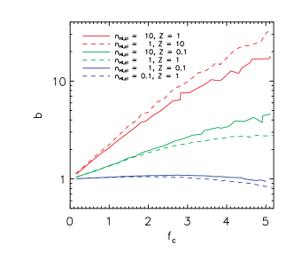
Figure 2.— EW boost $b$ as a function of covering factor $f_{\mathrm{c}}$, for various values of cloud Hi densities $n_{\textrm{{\scriptsize H}{\tiny\hskip 0.28453ptI},cl}}$ and metallicites $Z$. Lines with the same color share the same value of dust optical depth per cloud: blue, green, and red denote $\tau_{\mathrm{a,cl}}\simeq 0.02$, 0.2, and 2, respectively. For these simulations, the number of clouds and the galaxy radius was $N_{\mathrm{cl}}=100$–50 000 and $r_{\mathrm{gal}}=2$–10 kpc. Densities are given in cm^-3, and metallicites in terms of $Z_{\odot}$.

The boosts are seen to follow an approximate log-normal relation, where different combinations of $n_{\textrm{{\scriptsize H}{\tiny\hskip 0.28453ptI},cl}}$ and $Z$ with equal dust optical depths lie roughly on the same line. At fixed $Z$, larger Hi densities result in larger boosts. The Ly$\alpha$ photons are exposed to the same amount of extinction, but since $\langle\tau_{\mathrm{a}}\rangle$ is larger, the continuum is reduced more. At fixed $n_{\textrm{{\scriptsize H}{\tiny\hskip 0.28453ptI},cl}}$, a larger $Z$ also results in a larger boost due to the higher $\langle\tau_{\mathrm{a}}\rangle$, but since for each cloud interaction a Ly$\alpha$ experiences a larger probability of being absorbed, combinations with high $Z$ have smaller boosts than those with high $n_{\textrm{{\scriptsize H}{\tiny\hskip 0.28453ptI},cl}}$. This is especially true at large values of $f_{\mathrm{c}}$, where the Ly$\alpha$ photons interact with many clouds.

3.2. Cloud hydrogen density

To shield the Ly$\alpha$ photon from the dust, the clouds must be highly optically thick in hydrogen. Since non-absorbed photons are usually reflected after only a handful of scatterings, in principle the clouds could have an optical depth of only a few, although in that case, for realistic metallicites, the dust optical depth would be so low that the continuum passes unhindered through the clouds.

Figure 3 shows how the magnitude of the boost depends on the Hi (column) density of the clouds. Note that for a given series of simulations, the metallicity has been held fixed, meaning that $\langle\tau_{\mathrm{a}}\rangle$ increases with increasing $N_{\textrm{{\scriptsize H}{\tiny\hskip 0.28453ptI},cl}}$.

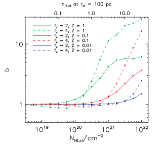
Figure 3.— EW boost $b$ as a function of neutral hydrogen column density $N_{\textrm{{\scriptsize H}{\tiny\hskip 0.28453ptI},cl}}$ of the individual clouds, as measured from the center to the surface of a cloud, for different gas metallicites. The upper $x$ axis gives the corresponding number densities in cm^-3 in the case of $r_{\mathrm{cl}}=100$ pc. Metallicities are given in terms of $Z_{\odot}$. The simulations for which $\mbox{$f_{\mathrm{c}}$}\sim 4$ have been realized simply using $N_{\mathrm{cl}}=13\,000$.

Even for Solar metallicity, the EW boost is seen to set in only after $N_{\textrm{{\scriptsize H}{\tiny\hskip 0.28453ptI},cl}}$ surpasses approximately $10^{20}$ cm^-2, while, say, ten times lower metallicity requires ten times higher $N_{\textrm{{\scriptsize H}{\tiny\hskip 0.28453ptI},cl}}$. The critical value for a noticeable boost is found where $N_{\textrm{{\scriptsize H}{\tiny\hskip 0.28453ptI},cl}}$ and $Z$ conspire to a dust optical depth of order unity. For very high values of $N_{\textrm{{\scriptsize H}{\tiny\hskip 0.28453ptI},cl}}$ the clouds become so optically thick in dust to continuum such that the calculated EWs become rather noisy.

3.3. Dust contents in the clouds

The density of dust scales both with metallicity and Hi density. Increasing the gas density in the clouds will increase the dust density accordingly. This does not change the surface of a cloud from the point of view of a Ly$\alpha$ photon, but the continuum photons experiences a larger total optical depth of dust, and thus the boost increases. For a given Hi density, increasing the metallicity results in a higher boost. These relations are shown in LABEL:Z.

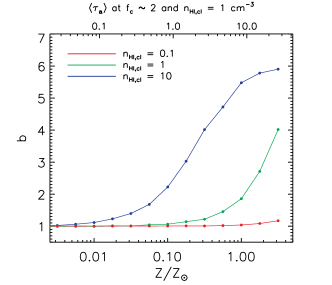
Figure 4.— EW boost $b$ as a function of gas metallicity $Z$ — which can be taken as a proxy for $\langle\tau_{\mathrm{a}}\rangle$ — for different Hi densities $n_{\textrm{{\scriptsize H}{\tiny\hskip 0.28453ptI},cl}}$ of the clouds.

As expected, larger Hi densities result in larger boosts, but for sufficiently low metallicites the boost will disappear. Again, the critical value of $Z$ is the metallicity required for the optical depth of dust to be of order unity. For the adopted cloud size of 100 pc, this corresponds to the product $n_{\textrm{{\scriptsize H}{\tiny\hskip 0.28453ptI}}}\,Z/\mbox{$Z_{\odot}$}\sim 1$, which is indeed seen in LABEL:Z.

3.4. Cloud size distribution

In the previous simulations the cloud radii were held constant at $r_{\mathrm{cl}}=100$ pc. As N91 proposed and HO06 confirmed through their numerical model, the covering factor rather than the actual shape and size of the clouds is the important parameter controlling the RT of the Ly$\alpha$ photons. For the continuum, however, doubling the cloud radius at constant $f_{\mathrm{c}}$ doubles the dust optical depth, thus increasing the boost. In LABEL:beta_and_rcl we investigate the dependency of the boost on cloud sizes, as well as on cloud size distributions $P(r_{\mathrm{cl}})\propto r_{\mathrm{cl}}^{-\beta}$.

Figure 5.— Lower $x$ axis and red lines: EW boost $b$ as a function of cloud radius $r_{\mathrm{cl}}$, maintaining constant covering factor $f_{\mathrm{c}}$ (solid) and a constant total Hi mass (dashed). Upper $x$ axis and green line: EW boost as a function of cloud size distribution power-law index $\beta$, for minimum and maximum cloud radii $r_{\mathrm{min}}=20$ pc and $r_{\mathrm{max}}=200$ pc, at constant $f_{\mathrm{c}}$.

The dependency on slope $\beta$ is seen to be small. In the simulations with varying cloud radii, the slope was held constant at $\beta=2$. This value was chosen to follow HO06.

Increasing $r_{\mathrm{cl}}$ or decreasing $\beta$ at constant $f_{\mathrm{c}}$ both corresponds to in increasing the $\langle\tau_{\mathrm{d}}\rangle$ and hence $b$, although it is seen that changes in $\beta$ affects $b$ only minutely. On the other hand, changing the cloud sizes but maintaining a constant total Hi mass implies a constant $\langle\tau_{\mathrm{d}}\rangle$, and hence a constant continuum escape fraction. Consequently, the boost does not change for $r_{\mathrm{cl}}\gtrsim 100$ pc, but at lower $r_{\mathrm{cl}}$ the number of times that the Ly$\alpha$ photon interact with clouds ($N_{0}$) becomes so large that the Ly$\alpha$ escape fraction decreases considerably, reducing the boost.

3.5. Cloud velocity dispersion

The very concept of the boost hinges on the fact that neutral gas shields photons close to the line center from the dust. But if a given cloud as a whole has a non-vanishing bulk velocity, the entire spectrum is Doppler shifted in the reference frame of the cloud, and for sufficiently large velocities, all line photons suddenly are no longer in resonance. In general, Hi regions may be expected to exhibit such macroscopic motions, described by a cloud velocity dispersion $\sigma_{V,\textrm{cl}}$.

Figure 6 demonstrates that this is indeed the case; for $\mbox{$\sigma_{V,\textrm{cl}}$}\gtrsim 100$ ${\rm km\,s^{-1}}$, the fiducial model is seen to be incapable of boosting the EW. Moreover, whereas in the case of $\mbox{$\sigma_{V,\textrm{cl}}$}=0$ a higher covering factor results in a larger boost, introducing random cloud motion reduces the boost even faster; for $f_{\mathrm{c}}$ twice that of the fiducial model, the boost vanishes already for $\mbox{$\sigma_{V,\textrm{cl}}$}\gtrsim 30$ ${\rm km\,s^{-1}}$.

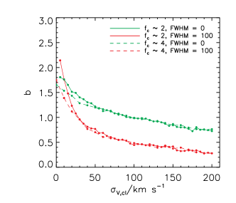
Figure 6.— EW boost as a function of cloud velocity dispersion $\sigma_{V,\textrm{cl}}$, for zero-width (solid) and broadened (dashed) emission, in galaxies of $\mbox{$f_{\mathrm{c}}$}\sim 2$ (green) and 4 (red).

3.6. Cloud gas temperature

Increasing the gas temperature $T_{\mathrm{cl}}$ in the clouds means less atoms with the right velocity for scattering photons exactly at the line center, in return for more atoms available for scattering off center photons. Photons in the wings of the line, however, do not care about the gas temperature, since the profile here is given by natural broadening. Even so, the difference in the effective cross section of the atoms is not very large. The consequence is that, for increasing $T_{\mathrm{cl}}$, the photons penetrate slightly deeper into the cloud, but not enough to affect the boost, as seen in LABEL:T_cl.

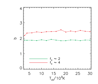
Figure 7.— EW boost as a function of cloud gas temperature $T_{\mathrm{cl}}$ (including also small scale turbulence) for a covering factor $\mbox{$f_{\mathrm{c}}$}\sim 2$ (green) and $\mbox{$f_{\mathrm{c}}$}\sim 4$ (red).

The only difference is that the line profile of the escaping radation is somewhat broadened.

3.7. Galactic outflows and infall

Gas elements also move in large-scale, collective motions, seen e.g. in galactic outflows (Johnson & Axford, 1971; Rupke et al., 2002; Shapley et al., 2003; Veilleux et al., 2005). For the same reason as in the previous section, such motions should act such as to diminish the boost. This stands in contrast to what is expected (Kunth et al., 1998; Dijkstra & Wyithe, 2010) for a more homogeneous shell of gas being expelled from the galaxy, surrounding a central source and covering the full sky. In that case, the Ly$\alpha$ photons that would otherwise have to scatter their way through the shell, being very vulnerable to dust absorption, may be shifted away from the line center and escape through the shell with minimal absorption.

Figure 8 shows how the EW boost depends on the expansion velocity $V_{\mathrm{out}}$. The wind speed is a function of distance $r$ from the center and is modelled assumed that the gas elements receive an acceleration $a\propto r^{-\alpha}$ (Steidel et al., 2010; Dijkstra & Kramer, 2012). The speed thus increases from 0 at $r=0$ to the terminal velocity $V_{\mathrm{out}}$at $r=r_{\mathrm{gal}}$. Note, however, that the exact wind profile is not a major determinant of the resulting boost.

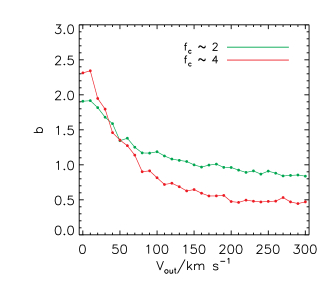
Figure 8.— EW boost as a function of terminal outflow expansion velocity $V_{\mathrm{out}}$for covering factors $\mbox{$f_{\mathrm{c}}$}\sim 2$ (green) and $\sim 4$ red.

The curves in LABEL:wind resemble those in LABEL:sigV, although they are somewhat more shallow. The reason is that a photon bouncing off of a cloud in a galactic wind will, in general, upon its next encounter with a cloud, meet a cloud with roughly the same velocity. In the case of random motions, the relative velocity of the next cloud may be very high, increasing the probability of the photon being absorbed.

For reasons of symmetry, in terms of $b$ the same results are obtained if the velocities are inverted, as would be the case for galactic gas accretion (e.g. Dijkstra et al., 2006b). The spectra, however, would be reflected about the line center.

3.8. ICM hydrogen density

Thus far, we have assumed an ICM completely void of both dust and neutral gas. Due to the high temperature of the ICM, the hydrogen is expected to be quite highly ionized. Similarly, due to the high temperature, as well as the stronger ionizing UV radiation field, dust may be expected to be partly depleted. However, even a single scattering in the ICM may be fatal to a Ly$\alpha$ photon: Exactly because of the high temperature, a scattering event in the ICM is likely to occur on a high-velocity atom moving more or less perpendicular to the path of the photon, such that the velocity relative to the trajectory of the photon is small. Unless the photon is scattered close to (or opposite to) the same direction, it will be highly Doppler-shifted, such that next time it encounters a cloud, it will penetrate deeply into the dusty medium, with a higher probability of being absorbed. This effect is investigated further in Sec. 3.10.

For our fiducial model’s radius of $r_{\mathrm{gal}}=5$ kpc, an optical depth of order unity in the ICM for a line center photon is reached for an Hi density $n_{\textrm{{\scriptsize H}{\tiny\hskip 0.28453ptI}}}\sim 10^{-8}$ cm^-3. Due to the resonance nature of the scattering, somewhat higher densities are allowed as soon as the photon has diffused a few Doppler width from the line center. This effect is visible if LABEL:NHI_ICM, where the boost is shown as a function of ICM Hi density for different cloud densities and metallicites.

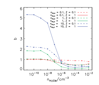
Figure 9.— EW boost $b$ as a function of Hi density $N_{\textrm{{\scriptsize H}{\tiny\hskip 0.28453ptI},ICM}}$ in the ICM. Results are show in red, green, and blue for cloud number densities $n_{\textrm{{\scriptsize H}{\tiny\hskip 0.28453ptI},cl}}=0.1$, 1, and 10 cm^-3, respectively, in combination with cloud metallicites $Z=0.1$ $Z_{\odot}$(dashed) and 1 $Z_{\odot}$ (solid).

3.9. ICM dust density

The neglect of dust in the ICM may be justified by the fact that dust grains will tend to get destroyed in hot and ionized media. Nevertheless, dust does exist in Hii regions, albeit generally at lower densities. For an increasing covering factor the photons’ paths through the ICM is increased as they walk randomly out through the galaxy. The mean free path between each cloud interaction is $1/\mbox{$f_{\mathrm{c}}$}$, while the average number of cloud interactions is $N_{0}=\mbox{$f_{\mathrm{c}}$}^{2}+\frac{4}{5}\mbox{$f_{\mathrm{c}}$}$ (see App. A.4). Thus, the average path length for a photon out of our fiducial model of $r_{\mathrm{gal}}=5$ kpc is $\langle d_{\mathrm{tot}}\rangle\simeq 14$ kpc. For a density of 0.01 cm^-3, $Z=\mbox{$Z_{\odot}$}$, and no dust destruction, the total optical depth of dust actually reaches $\langle\tau_{\mathrm{ICM}}\rangle\sim 0.2$. For larger densities $r_{\mathrm{gal}}$ and $f_{\mathrm{c}}$, $\langle\tau_{\mathrm{ICM}}\rangle$ could exceed unity, while if part of the dust is destroyed, it may be neglected altogether.

Figure 10 shows the effect of dust in the ICM for various densities, galaxy radii, and dust depletion factors. The important quantity is the number density of dust, which is proportional to the product of total density, metallicity, and dust-to-metal ratio $\xi_{\textrm{d}}$; that is, a given dust density can be realized in several ways. While in predominantly neutral regions, $\xi_{\textrm{d}}$ is rather constant (see discussion in Sec. 4.4 and Sec. 4.8). Accordingly, the boost is shown as a function of the product of $Z$ and $\xi_{\textrm{d}}$, for different total hydrogen densities.

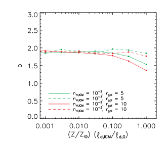
Figure 10.— EW boost $b$ as a function of dust density in the intercloud medium, parametrized through the amount of metals in the form of dust, $(Z/\mbox{$Z_{\odot}$})\times(\xi_{\textrm{d,ICM}}/\xi_{\mathrm{d,0}})$, where the last term is the dust-to-metal ratio in terms of the values typically found in the predominantly neutral environments from where the dust extinction curve is taken (here the SMC). Results are shown for galaxies of $r_{\mathrm{gal}}=5$ (green) and 10 kpc (red), in combination with total (neutral + ionized) hydrogen density $n_{\textrm{H,ICM}}=10^{-3}$ (dashed) and $n_{\textrm{H,ICM}}=10^{-2}$ cm^-3 (solid).

Indeed, ICM dust is seen to be important only for rather high ICM densities, large galaxies, and low dust depletion factors. Thus we see that the most crucial factor of the Neufeld mechanism is not, as it is often laid out, that the Ly$\alpha$ photons are confined to a dustless medium but rather that are confined to a medium of low density but possibly with the same dust-to-gas ratio, and high ionization fraction.

3.10. ICM gas temperature

As mentioned in Sec. 3.8, although scatterings in the ICM evidently are rare a single such event may easily result in the subsequent absorption of the photon. Figure 11 explores this effect, but it is seen that only for rather high values of $n_{\textrm{{\scriptsize H}{\tiny\hskip 0.28453ptI},ICM}}$, the boost decreases significantly.

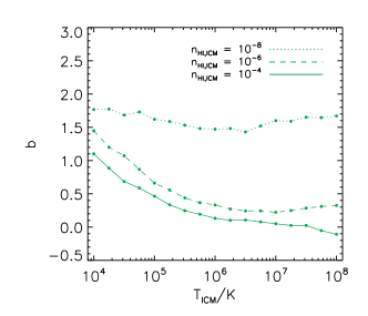
Figure 11.— EW boost as a function of temperature $T_{\mathrm{ICM}}$ in the ICM, for neutral hydrogen densities $n_{\textrm{{\scriptsize H}{\tiny\hskip 0.28453ptI},ICM}}=10^{-8}$ (dotted), $n_{\textrm{{\scriptsize H}{\tiny\hskip 0.28453ptI},ICM}}=10^{-6}$ (dashed), and $n_{\textrm{{\scriptsize H}{\tiny\hskip 0.28453ptI},ICM}}=10^{-4}$ (solid) cm^-3.

For low densities, scatterings are so rare that even though some photons are absorbed, it does not affect the net result much. For very high temperatures, the boost increases again, since the number of atoms available with the right velocity to scatter a photon becomes too small.

3.11. Location of emission

Although star formation tends to be centrally located (e.g. Fruchter et al., 2006), obviously the photons are not emitted from a point source in reality. However, as long as the initial emission direction is isotropically distributed, photons emitted in the outskirts of the galaxy may be emitted both in an outward direction, being subject to a lower covering factor and thus a smaller boost, or toward the center, resulting in a higher covering factor and higher boost. As the number of cloud interactions scale non-linearly with $f_{\mathrm{c}}$, however, an extended emission profile does result in a slightly lower boost, although the effect is miniscule, as seen in LABEL:grad.

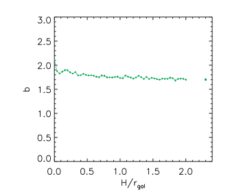
Figure 12.— The effect of an extended emission, as given by an exponentially decreasing emission site PDF of the form $P(r)\propto e^{-r/H}$, where $r$ is the distance from the center of the galaxy, and $H$ is the scale length. The rightmost point shows the boost for $H\rightarrow\infty$, i.e. for a completely homogeneous distribution of sources.

While the extended emission relaxes the notion of a central point source, all photons were still emitted from the ICM, as in the case of the central source in all previous sections. However, as the Ly$\alpha$ radiation is assumed to originate from gas surrounding young stars, which form from gas clouds that have recently cooled sufficiently to initiate star formation, it is probably more realistic to have at least a fraction of the photons originating from within the clouds. In LABEL:Pcl we investigate how the EW boost changes for an increasing correlation of the photon sources with the clouds.

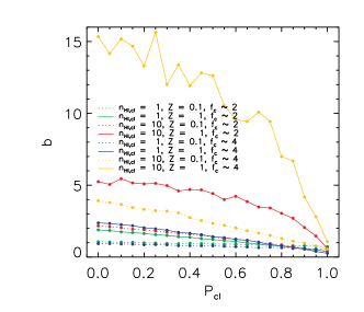
Figure 13.— EW boost $b$ as a function of probability $P_{\mathrm{cl}}$ for a photon to be emitted from inside a cloud. An emission PDF with a scale length of $H=1$ kpc has been adopted. For $P_{\mathrm{cl}}=0$, the model reduces to the fiducial model, except for the somewhat extended emission which has only a modest influence on $b$ (cf. LABEL:grad). For $P_{\mathrm{cl}}=1$, all photons are emitted from the interior of clouds. Results are show for all combinations of $\mbox{$f_{\mathrm{c}}$}\sim 2,4$, $n_{\textrm{{\scriptsize H}{\tiny\hskip 0.28453ptI},cl}}/\mbox{cm${}^{-3}$}=1,10$, and $Z/\mbox{$Z_{\odot}$}=0.1,1$.

As expected, taking this effect into account diminishes the boost, as the path out of a cloud is longer for a Ly$\alpha$ photon than for a continuum photon.

3.12. Intrinsic line profile

In the fiducial model, all Ly$\alpha$ photons are emitted exactly in the line center, i.e. as a delta function. In reality, the intrinsic line will have a finite width, which is convolution between the natural, Lorentzian line profile and the thermal, Gaussian distribution of the atom velocities. Moreover, macroscopic motion of the gas parcels emitting the photon will cause an effective broadening of the line. As the temperature of the emitting gas is of the order $10^{4}$ K, corresponding to a line width of $\sim 10$ ${\rm km\,s^{-1}}$, the macroscopic motion may dominate over the thermal (see Sec. 4.1). From non-resonant lines such as H$\alpha$, we know that the intrinsic line width may easily reach tens of ${\rm km\,s^{-1}}$, i.e. several Doppler widths. As photons born this far from the line center are not efficiently shielded from the dust, they are more prone to dust absorption.

The effect of a broadened emission line profile is shown in LABEL:fwhm.

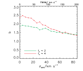
Figure 14.— EW boost $b$ as a function of line width $\sigma_{\mathrm{em}}$ for covering factors $\mbox{$f_{\mathrm{c}}$}\simeq 2$ (green) and 4 (red).

4. Toward a realistic model

Whereas the fiducial model in the previous section was not chosen to be particular realistic, but rather to roughly resemble the original Neufeld scenario, we now proceed to investigate what values of the physical parameters we in fact expect to meet in real LAEs. In building a “realistic” model, it should be kept in mind that several of the input parameters are mutually dependent. For instance, under the assumption of approximate pressure equilibrium, the temperatures and densities are related as $n_{\mathrm{tot,cl}}T_{\mathrm{cl}}\sim n_{\mathrm{tot,ICM}}T_{\mathrm{ICM}}$, where subscripts “tot” refer to the total number density of all particles. The Hi densities are then given by the ionization fractions which, in turn, depend on not only temperature, but also the chemical composition, i.e. on metallicity. Note, however, that due to very different cooling time scales of the WNM and HIM, the different phases of the ISM need not be in thermal equilibrium. Furthermore, the dependencies of some of the parameters may actually serve such as to counteract a boost. For instance, a larger galaxy in general entail a larger $f_{\mathrm{c}}$, which may increase $b$, but since the larger mass also typically implies a larger $\sigma_{V,\textrm{cl}}$, $b$ is quickly reduced again. Similarly, although a increased metallicity tends to increase $b$, metals also donate free electrons, which aids to increase the neutral fraction of hydrogen in the ICM, thus decreasing $b$.

The approach taken here is to identify for each parameter the minimum and the maximum values conceived to be encountered in LAEs, as well as more typical ranges. Subsequently a series of RT simulations is run with the physical parameters taking random values in the chosen ranges, and finally regions of high and low likelihood are identified in the parameter space, exploring whether any of these models lead to a significant boost.

LAEs span a wide range of physical characteristics, and in many aspects it does not make sense to speak about a “typical LAE”. It is often stated that LAEs are quite young, fairly small, relatively highly star-forming galaxies of rather low metallicity and dust contents. However, one must bear in mind that many of these aspects are a consequence of the selection criterion picking out objects at high redshifts, i.e. at early epochs. In the following sections, values and ranges of the relevant parameters argued to be more or less representative of LAEs are summarized from the literature. An overview of the values is found in Tab. 1 on page 1.

4.1. Cloud hydrogen density and temperature

Gas does not cool equally well at all temperatures. Rather the cooling function exhibit several plateaus at which the gas temperature tends to settle. This is part of the reason for the different phases of the ISM; for gas which is in rough pressure equilibrium, the densities of the phases are set by their temperature, and thus, although variations do exist, they are not expected to span many orders of magnitude within a given phase. In the WNM, to which the clouds in the model correspond, characteristic hydrogen densities are 0.2–0.5 (e.g. Carilli et al., 1998; Ferrière, 2001; Gloeckler & Geiss, 2004) — typically probed by Hi 21 cm emission — with a neutral fraction close to unity. At low (high) pressure, $n_{\textrm{{\scriptsize H}{\tiny\hskip 0.28453ptI}}}$ may reach values of $\sim 0.02$ (3) cm^-3(Wolfire et al., 2003). If densities rise much above $\sim 1$ particle cm^-3, cooling becomes so efficient that the gas will tend to contract further to a cold neutral medium (CNM) and molecular clouds, thus quickly decreasing $f_{\mathrm{c}}$. The temperature of the WNM is of the order $10^{4}$ K, ranging from 8 000 K to 12 000. Since small scale turbulence effectively broadens the line in the same way as thermal motion, this process can be taken into account using a higher temperature. Turbulence is usually of the order of (a few times) the speed of sound (e.g. Gaensler et al., 2011) which, in turn, is the same order as the thermal motion. The effect can thus be simulated by letting $T=2$–$3\times 10^{4}$ K. Note also that much of the WNM may be in a thermally unstable phase (Heiles & Troland, 2003), reaching temperatures below 5 000 K.

4.2. ICM hydrogen density and temperature

Surrounding the neutral gas is the HIM, heated and ionized to a large degree by supernova shock waves sweeping through the ISM. Expanding due to the larger pressure, and thus diluting, the cooling timescales are so long that temperatures of $5\times 10^{5}$–$5\times 10^{6}$ K and higher is easily maintained (Brinks et al., 2000; Tüllmann et al., 2006, 2008). Densities in the range $10^{-3}$ to $10^{-2}$ are typical here (Dopita & Sutherland, 2003; Ferrière, 2001), but since the fraction of neutral hydrogen at these temperatures is of the order $x_{\textrm{{\scriptsize H}{\tiny\hskip 0.28453ptI},ICM}}\sim 10^{-8}$–$10^{-5}$ (House, 1964; Sutherland & Dopita, 1993), scattering in the ICM is very rare. These properties are usually probed through X-ray emission (e.g. Tüllmann et al., 2006), or absorption lines of highly ionized metals (e.g. Park et al., 2009). Note that the shock waves push the phases out of equilibrium and may in fact dominate the state of the ISM (de Avillez & Breitschwerdt, 2005).

4.3. Covering factor

A typical covering factor is difficult to establish, but a hint is provided by spectra of sources lying behind intervening galaxies. For instance, Noterdaeme et al. (2012) fit low-ionization absorption lines such as Siii — originating from cool clouds — in a quasar spectrum, the line of sight toward which passes through a DLA lying at $z=2.2$, with 5–8 components. The impact parameter of the sightline with respect to the central emission of the DLA galaxy counterpart is pretty small ($\lesssim 1$ kpc), and thus in this case the covering factor is roughly $\mbox{$f_{\mathrm{c}}$}=2.5$–4.

In the Milky Way (MW), the number of neutral clouds per kpc in the plane is roughly 4–8 (Knude, 1979, 1981; Franco, 2012). Although this implies a high covering factor along a sightline in the plane, perpendicular hereto the covering factor is only of order unity. Since the disk has formed from a collapsed sphere, one may expect a smaller number of clouds per kpc for a spherical system. For instance, the scale height of the MW’s WNM is approximately $h=300$ pc and its radius is $R_{\mathrm{MW}}\sim 15$ kpc (Binney & Merrifield, 1998); distributing the clouds over a sphere of the same radius reduces the crowdedness of clouds by a factor of $\sim R_{\mathrm{MW}}/h=50$.

4.4. Cloud metallicity and dust density

Generally lying at high redshifts where metals have had less time to build up, LAEs tend to have lower metallicities, and hence dust densities, than local galaxies. Measured values of $Z$ range from metallicities as low as $\sim 10^{-2}\mbox{$Z_{\odot}$}$ to values similar to local values, and in some cases even supersolar metallicities have been found at high redshifts (e.g. Acquaviva et al., 2012). In a survey of $\sim 10^{3}$ LAEs at $z=2.2$, Nakajima et al. (2012) found a lower limit for the average metallicity of a LAE of $Z=0.09\mbox{$Z_{\odot}$}$. Even low-redshift LAEs tend to have modest metallicities ($Z\simeq 0.1$–1 Giavalisco et al., 1996; Östlin et al., 2009).

Correspondingly, measured color excesses tend to be modest. For example, at $z\sim 3$ Gronwall et al. (2007) and Pirzkal et al. (2007) found $E(B-V)$’s lying approximately in the range 0.01 to 0.1. Verhamme et al. (2008) found similar values by fitting Ly$\alpha$ line profiles using the Ly$\alpha$ RT code MCLya (Verhamme et al., 2006). At $z=2.2$, Hayes et al. (2010) found values spanning all the way from 0 to $\sim 0.3$. For comparison, our fiducial model has $\mbox{$E(B-V)$}=0.05$.

In our model we assume that the dust-to-metal ratio $\xi_{\textrm{d,cl}}$ in the clouds is equal to that of our reference extinction curve, such that $\tau_{\mathrm{d}}$ scales linearly with $Z$. Observations of $\xi_{\textrm{d,cl}}$ at high redshifts are sparse, but tend to be similar (e.g. Pettini et al., 1997; Savaglio et al., 2003) or slightly lower. Various analytical and numerical calculations predict a metallicity-dependent evolution of the dust-to-metal ratio, such that $\xi_{\textrm{d,cl}}$ reaches present-day values only after timescales of 10–100 Myr (Gall et al., 2011) or even several Gyr (Inoue, 2003, see also Mattsson (2011)). Moreover, measurements in the local but very low-metallicity galaxy I Zw 18 indicate that $\xi_{\textrm{d,cl}}$ is lower in such galaxies. Since we have used the extinction law of the SMC, which is also a low-metallicity galaxy with a rather young stellar population, we expect that its extinction will not be substantially different from that of high-redshift galaxies.

4.5. Cloud velocity dispersion

From the virial theorem, the components of a galaxy of mass $M$ and radius $r$ will have characteristic velocities of the order $\mbox{$\sigma_{V,\textrm{cl}}$}=\sqrt{GM/Cr}$, where the factor $C$ depends on the geometry and the actual mass distribution, as well as on whether the system is rotation- or dispersion-dominated (Binney & Tremaine, 2008). For dispersion-dominated galaxies, $M$ refers to the total, dynamical mass of the system, and $C\simeq 6.7$ for various galactic mass distributions (Förster Schreiber et al., 2009). For rotation-dominated galaxies, the appropriate mass is the mass enclosed within $r$, and $C\simeq 2.25$, again averaged over various galactic mass distribution models (Epinat et al., 2009).

Measured values of the Hi velocity dispersion, or of the stellar velocity dispersion which arguably reflects the velocity field of the gaseous components, range from $\sim 10$–$30$ ${\rm km\,s^{-1}}$for dwarf galaxies (e.g. Peterson & Caldwell, 1993; van Zee et al., 1998) to several hundred ${\rm km\,s^{-1}}$ for large ellipticals (e.g. McElroy, 1995). Note that observationally what is measured is the dispersion along a line of sight, or an average of many lines of sight, and hence correspond to the dispersion in one dimension. If there is no preferred direction of motion, the three-dimensional velocity dispersion, which is what is referred to in Sec. 3.5, is a factor $\sqrt{3}$ times higher.

Our fiducial model has a total Hi mass of $6.7\times 10^{8}\,\mbox{$M_{\odot}$}$. For small galaxies, the ratio of Hi to the total, dynamical mass is roughly 0.1 (Skillman et al., 1987; van Zee et al., 1997, 1998). Thus, the velocity dispersion should be approximately 50 ${\rm km\,s^{-1}}$.

At high redshift, most galaxies may not yet have had time to form a disk, and may thus be expected to be dispersion-dominated. For galaxies which eventually settle into a disk, the velocity dispersion tends to decrease (e.g. Thomas et al., 2012). For instance, for intermediate- to late-type spirals, Bershady et al. (2011) found that the central vertical velocity dispersion is $\sim 1/4$ of the maximum rotation speed.

The preceding reasoning dealt with the overall velocity dispersion of the galaxy’s components. For relaxed disks, these could be correlated in phase space, such that locally to a given photon’s emission site the first few clouds encountered will have a lower relative velocity. With a lower limit of 5 ${\rm km\,s^{-1}}$, however, we believe that a realistic threshold has been met; for instance, in the MW the dispersions in peculiar motion of local stars with respect to the local standard of rest is $\sim 20$ ${\rm km\,s^{-1}}$ (Schönrich et al., 2010).

The velocity dispersion of the gaseous component might be expected to be smaller than the stellar velocity dispersion, however, but in The Hi Nearby Galaxy Survey (THINGS), the galaxies, which are almost exclusively disk galaxies, exhibit velocity dispersions between 10.1 and 24.3 ${\rm km\,s^{-1}}$, with a mean of $16.8\pm 4.3$ ${\rm km\,s^{-1}}$ (Ianjamasimanana et al., 2012).

4.6. Galactic outflow velocity

Although not ubiquitous, galactic winds seem to be rather common in high-redshift galaxies. The outflows are produced by the kinetic and/or thermal feedback of massive stars and supernovae on the ISM. Radiation pressure and heating engender expanding bubbles of primarily ionized gas that sweep up interstellar material, eventually escaping the galaxy (or possibly re-entering the system after having reached several virial radii) (Heckman, 2002). Outflows are usually detected through low-ionization absorption lines such as Mgii and Feii which appear blueshifted with respect to the systemic velocity. Typical values are of the order 100 ${\rm km\,s^{-1}}$ (e.g. Pettini et al., 2001; Rubin et al., 2011), but range all the way from 0 and up to $\sim 1$–$2000$ ${\rm km\,s^{-1}}$(e.g. Shapley et al., 2003).

Various models for galactic outflows have been put forward: Orsi et al. (2012) equate $V_{\mathrm{out}}$with the circular velocity, which is of the same order as $\sigma_{V,\textrm{cl}}$, discussed in the previous section. Bertone et al. (2005) and Garel et al. (2012) apply a weak dependency on SFR, with $\mbox{$V_{\mathrm{out}}$}\propto\textrm{SFR}^{0.145}$, where the SFR is given is $M_{\odot}$ yr^-1, and the constant of proportionality is $\simeq 300$–1000 ${\rm km\,s^{-1}}$.

In the context of LAEs, the effect of an outflow is to diminish the blue peak of the otherwise symmetric, double-peaked line profile. This is noticable already $\sim 10$ ${\rm km\,s^{-1}}$, and by $\sim 100$ ${\rm km\,s^{-1}}$, the blue peak may be erased altogether (e.g. Dijkstra et al., 2006a). Most high-redshift LAE profile observations have resulted in the well-known, asymmetric red peak only. However, using sufficiently high resolution, $R\gtrsim 1$–2000, it seems that a significant fraction (20–50%) of LAEs actually show at least signatures of a blue peak, indicating only modest outflow velocities (Venemans et al., 2005; Tapken et al., 2007; Kulas et al., 2012; Yamada et al., 2012).

This hypothesis is in qualitative concord with the recent findings of Hashimoto et al. (2012), who interpret the smaller offset of LAE Ly$\alpha$ lines with respect to the systemic velocity, compared with those of LBGs, as being due to smaller outflow velocities. Note, however, that the line offset to a large degree depends on the column density, which due to the generally much higher gas mass of LBGs naturally will be larger.

For the reasons given above, and since a large outflow velocity was found to quicky destroy the boost anyway, we will restrain ourselves to investigating rather small values of $V_{\mathrm{out}}$, from 0 to 100 ${\rm km\,s^{-1}}$.

4.7. Emission sites

Since evidently the extend of the photon-emitting region is not of major importance (see Sec. 3.11), for simplicity we will confine our grid of models to one value only, viz. $H_{\mathrm{em}}=1$ kpc. This value is roughly equal to the UV half-light radius of LAEs at redshifts $2\lesssim z\lesssim 6$ (see Fig. 2 of Malhotra et al., 2012).

The typical environment from which photons are emitted is more crucial. Originating in the Hi/Hii-boundaries surrounding massive stars, the concept of emitting the Ly$\alpha$ photons from the ICM is rather dubious. Massive stars are predominantly born in giant molecular clouds (GMCs; e.g. Garay & Lizano, 1999) Since such stars are short-lived, with lifetimes of but a few Myr, they are not expected to travel very far from the dense clouds from which they were born. This favors a high value of $P_{\mathrm{cl}}$, the probability of being emitted from a cloud rather than from the ICM. On the other hand the intense UV radiation carves out a Strömgren sphere, which reaches a size of the order of 10(s) pc in a few Myr (Hosokawa & Inutsuka, 2006; Gendelev & Krumholz, 2012). If they are matter-bounded rather than radiation-bounded, the Ly$\alpha$ photons start to stream freely out into the surrounding, lower-density medium.

Although Israel (1978) found that most massive stars are located in the outskirts of GMCs (in the MW), Waller et al. (1987) argue that they tend to be more centrally located, but that $\sim 30$% of the Hii regions used to probe O and B stars in reality are just parcels of ionized gas that was once in molecular form near the surface of its host cloud. On the other hand, Gendelev & Krumholz (2012) reason that internal turbulence in the GMCs creates filamentary structure so that any star has a high probability of being born near the surface.

Regardless of the massive stars being born deep in the GMCs, or being born closer to the edge so that blisters allow a high escape fraction of ionizing and hence Ly$\alpha$ photons, the GMCs themselves are usually embedded in the WNM. The density of the WNM being several orders of magnitude lower than the GMCs, a Strömgren sphere that breaks out of a GMC may be able to grow faster, faciliting escape into the ICM.

Massive star do also exist in exposed cluster, such as in the Pleiades. Although the stars necessarily are born in dense clouds, some stellar groups manage to ionize and blow away the neutral gas. Observations of this at high redshifts are difficult, but in the nearest 2 kpc of the Sun, Lada & Lada (2003) estimate the (lower limit) birthrate of embedded clusters to be 2–4 Myr^-1 kpc^-2, which is more than an order of magnitude higher than that of open clusters (0.25–0.45 Myr^-1 kpc^-2 Elmegreen & Clemens, 1985; Battinelli & Capuzzo-Dolcetta, 1991).

In a study of 45 GMCs in M33, Imara et al. (2011) found 29 to be spatially and kinematically coincident with a local peak in atomic gas, 13 to be kinematically coincident, but located near the edge or on a filament between two peaks, and the remaining three not to be associated with any high-density atomic gas. In the region NGC 602/N90 in the SMC, Gouliermis et al. (2012) found an “unusually large fraction” of 60% of the pre-main sequence stars to be clustered, while the rest are diffusely distributed in the intercluster area.

Additionally, in the MW 10–20% of all O stars are found in ultracompact Hii regions, still embedded in their natal molecular cloud (Churchwell, 1990).

From these considerations, we consider $P_{\mathrm{cl}}=0.1$ a lower value, 0.2–0.5 to be a more or less realistic value, and 0.9 to be a highest value.

4.8. ICM dust density

Since the various ways of destroying dust tend to correlate with processes that also ionize gas (collision, sputtering, sublimation, and evaporation), the dust-to-metal ratio $\xi_{\textrm{d}}$, and hence the dust-to-gas ratio, in ionized gas may be expected to be lower than in neutral regions. However, most extinction curves are obtained from sightlines crossing several phases of the ISM, although typically only the correlation of the extinction with the neutral hydrogen is probed. Hence, the variation of $\xi_{\textrm{d}}$ with $x_{\textrm{{\scriptsize H}{\tiny\hskip 0.28453ptI}}}$ is not well-constrained. Whereas $\xi_{\textrm{d}}$ in neutral gas seems to be more or less universal over both different phases, metallicities, and redshifts, the observations that do exist generally indicate a lower $\xi_{\textrm{d}}$ in regions of ionized gas, albeit with large variations. On the basis of a discussion of various such regions, Laursen et al. (2009b) argue (Sec. 2.1.1) that $\xi_{\textrm{d}}$ in these regions ranges between a factor of $10^{-4}$ lower than in the neutral phases, to values similar to these, but with typical values of $10^{-2}$ times lower. This is an average over several different types of Hii regions, in particular also the very dust-depleted IGM; in the HIM $\xi_{\textrm{d}}=10^{-1}$ may be more representative. A similar discussion was given recently by Paladini et al. (2012, Sec. 5), where also it is noted that the mere radiation pressure may be able to clear large volumes of dust.

4.9. Emission line width

The intrinsic Ly$\alpha$ line width is given by a convolution of the natural, thermal, and turbulent broadening. As discussed in Sec. 4.1, turbulence may dominate over thermal motions. Since scattering changes the line shape in a highly non-trivial way, Ly$\alpha$ line shape observations do not reveal the intrinsic shape. Instead the width of non-resonant lines such as H$\alpha$, which are produced in the same locations as Ly$\alpha$, arguably can be used as a probe. Since the emitting regions also exhibit larger-scale motions, however, when observing the line integrated over the full galaxy it will usually be much broader.

When galaxies are well resolved, the internal motion of cloud are more easily disentangled. In nearby galaxies, (Yang et al., 1994) found H$\alpha$ line widths (in terms of standard deviations) of 20–30 ${\rm km\,s^{-1}}$. At higher redshifts, using CO lines where large-scale motions have been removed, Swinbank et al. (2011) determine the internal velocity dispersion of the components of a starburst galaxy at $z=2.3$ to be 45–85 ${\rm km\,s^{-1}}$.

4.10. Cloud size distribution

As mentioned previously, the covering factor rather than the actual shapes and sizes of the clouds are the crucial factor in determining the boost. However, for $P_{\mathrm{cl}}>0$, the size of the clouds become important, as smaller clouds implies an easier escape from the first cloud. On the other hand, at a given covering factor a larger cloud size implies more attenuation of the continuum. In Sec. 3.4 we used $\beta=2$ when keeping $r_{\mathrm{cl}}$ constant in order to follow HO06. Measured slopes tend to be more shallow, $\beta\sim 1.6$ (Dickey & Garwood, 1989; Williams & McKee, 1997). Obviously, in reality the WNM does not consist of spherical clouds, so in order for the conclusions not to depend too much on the chosen cloud sizes, we will study a broad range of cloud sizes and distributions. Approximately half of the simulations will be run with fixed cloud size, both $r_{\mathrm{cl}}=30$ pc and $r_{\mathrm{cl}}=100$ pc, while the other half is run with $r_{\mathrm{cl}}=20$–200 pc and $\beta=1$–2.5. This cloud size range is roughly consistent with that of the LMC (Kim et al., 2003). Smaller cloud sizes probably requires further cooling, while larger clouds will get torn apart by large scale motion, at least in rotation-dominated objects (Newton, 1980).

5. Results

Having settled upon more or less realistic ranges of the parameters important for the RT, summarized in Tab. 1, a large number ($4\times 10^{4}$) of simulations is carried out in the many-dimensional parameter space $\mathscr{P}$ spanned by the parameters.

Table 1Summary of parameter values

Parameter	Full range	“Typical”	“Unusual”	Sec.
$n_{\textrm{{\scriptsize H}{\tiny\hskip 0.28453ptI},cl}}$	0.03–3	0.2–0.5	0.1–1	4.1
$T_{\mathrm{cl}}$	5$\times 10^{3}$–3$\times 10^{4}$	8 000–20 000	Full range	4.1
$Z$	0.03–2	0.05–0.3	0.03–1	4.4
$\sigma_{V,\textrm{cl}}$	5-100	30–50	10–80	4.5
$f_{\mathrm{c}}$	0.8–8	Full range	Full range	4.3
$r_{\mathrm{cl}}$	0.03–0.2	Full range	Full range	4.10
$\beta$	1–2.5	Full range	Full range	4.10
$n_{\textrm{{\scriptsize H}{\tiny\hskip 0.28453ptI},ICM}}$	$10^{-12}$–$10^{-6}$	$10^{-10}$–$10^{-7}$	Full range	4.2
$T_{\mathrm{ICM}}$	3$\times 10^{5}$–5$\times 10^{7}$	$10^{5.5}$–$10^{6.5}$	Full range	4.2
$V_{\mathrm{out}}$	0–100	10–50	Full range	4.6
$H_{\mathrm{em}}$	1	1	1	4.7
$P_{\mathrm{cl}}$	0–1	0.2–0.5	0.1–0.9	4.7
$\sigma_{\mathrm{em}}$	5–100	10–85	Full range	4.9
$r_{\mathrm{gal}}$	5, 10	5, 10	5, 10

Note. — Densities are given in cm^-3, metallicity in terms of the Solar value, velocities and line widths in ${\rm km\,s^{-1}}$, temperatures in Kelvin, distances in kpc.

Whereas in all previous simulations $10^{5}$ photons were used to ensure convergence, in order to be able to adequately sample $\mathscr{P}$, we use only $10^{3}$ photons per model. In most simulations, the resulting boost is accurate to within roughly 10%; in simulations where the continuum escape fraction is very low, usually implying a large boost, this tends to overestimate the boost. One hundred of such simulations were resimulated to convergence; of these, five were found to have underestimated $b$ by 20–30%, while the rest had overestimated $b$ by $\sim 0$–300%. However, as will be evident below, all of these models correspond to physically extremely unlikely models.

The results of the simulations are displayed in LABEL:real, where the boosts of all models are shown as a function of total, average column density $\langle N_{\textrm{{\scriptsize H}{\tiny\hskip 0.28453ptI}}}\rangle$ of neutral hydrogen, colored according to their metallicity.

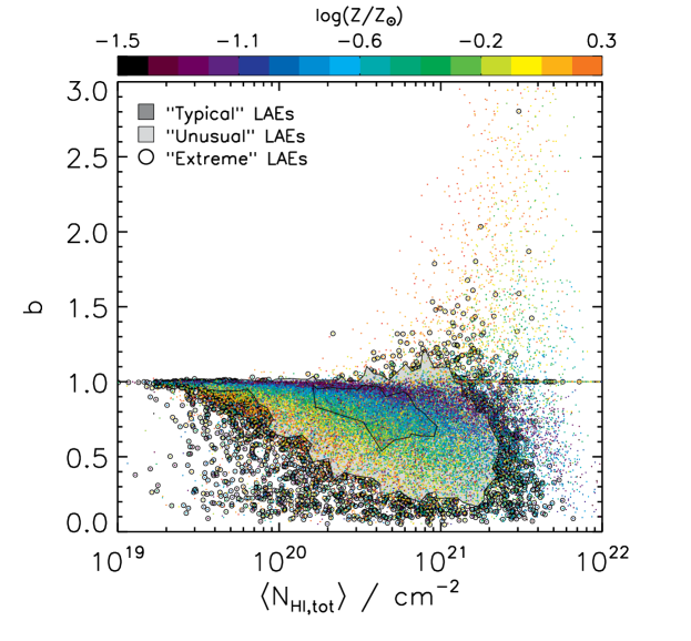
Figure 15.— “Likelihood map” of the obtained boosts for models with realistic and sub-realistic parameter values. The boost is shown, arbitrarily, as a function of average neutral hydrogen column density $\langle N_{\textrm{{\scriptsize H}{\tiny\hskip 0.28453ptI}}}\rangle$, as measured from the center to the surface of a galaxy. Each point represents a galaxy, the physical parameters of which are a realization of random values in the ranges discussed in Secs. 4.1 through 4.10 and summarized in Tab. 1. The metallicity of a galaxy is depicted by the color of the associated point. Models of “typical” and ”unusual” parameters all lie within the dark and light gray regions, respectively. The rest of the models have rather unrealistic parameters, but the ones that have either $n_{\textrm{{\scriptsize H}{\tiny\hskip 0.28453ptI},cl}}\leq 1.5$ cm^-3, $Z\leq 1.25$, $\mbox{$\sigma_{V,\textrm{cl}}$}\geq 10$ ${\rm km\,s^{-1}}$, or $P_{\mathrm{cl}}\geq 0.10$ are marked by black circles.

The gray-shaded contours indicate regions of likelihood, based on the parameter value ranges listed in column 2 and 3 of Tab. 1. “Typical LAE” models all lie within the dark gray area, while “unusual” models lie within the light gray area.

The remaining models all have rather unrealistic values. We have marked with black circles the ones for which nevertheless at least one of the following inequalities is true: $n_{\textrm{{\scriptsize H}{\tiny\hskip 0.28453ptI},cl}}\leq 1.5$ cm^-3, $Z\leq 1.25$, $\mbox{$\sigma_{V,\textrm{cl}}$}\geq 10$, or $P_{\mathrm{cl}}\geq 0.10$; these models are regarded as “extreme, but possibly conceivable”, while the remaining are regarded as “extreme and probably inconceivable”.

6. Discussion

By far, the majority of the models reveal a boost of $\lesssim 1$. Furthermore, the ones that do exhibit $b>1$ tend to have supersolar metallicity, very high cloud Hi densities ($\sim 5$–$10\times$ typical values), very low velocity fields (both $V_{\mathrm{out}}$ and $\sigma_{V,\textrm{cl}}$ are $<10$ ${\rm km\,s^{-1}}$), virtually empty intercloud media, and a high fraction ($>80$%) of photons born in the ICM.

Of the models labeled “extreme, but possibly conceivable” (indicated in LABEL:real by the black circles), twelve has resulted in a boost of $b>1.5$. Taking a closer look at these model reveals that they all lie close to the (admittedly somewhat arbitrary) threshold between “conceivable” and “inconceivable”. Moreover, although outflow velocity was not considered as a defining threshold, all except one have $\mbox{$V_{\mathrm{out}}$}\sim 1$ ${\rm km\,s^{-1}}$. One model has $\mbox{$V_{\mathrm{out}}$}=17$ ${\rm km\,s^{-1}}$, but has slightly supersolar metallicity ($Z=1.1\mbox{$Z_{\odot}$}$), low velocity dispersion ($\mbox{$\sigma_{V,\textrm{cl}}$}=14$ ${\rm km\,s^{-1}}$), low emission cloud-correlation ($P_{\mathrm{cl}}=0.15$), narrow intrinsic emission line ($\sigma_{\mathrm{em}}=15$ ${\rm km\,s^{-1}}$), high cloud densities ($n_{\textrm{{\scriptsize H}{\tiny\hskip 0.28453ptI},cl}}\simeq 1.5$ cm^-3) while virtually empty ICM ($n_{\textrm{{\scriptsize H}{\tiny\hskip 0.28453ptI},ICM}}\simeq 10^{-10}$ cm^-3).

The twelve models were all resimulated with $10^{5}$ photons. These resimulations reduced the value of the boost somewhat in all but one case (where it increased by a few percent). Furthermore, inspecting the emerging spectra (LABEL:spectra) shows that all models exhibit very narrow emission lines.

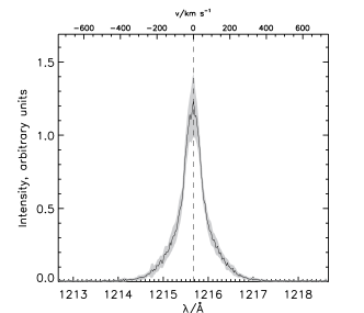
Figure 16.— Average spectrum (solid line) and 1$\sigma$ region (gray-shaded area) of the marginally realistic models giving a boost larger than $b=1.5$. With an average (maximum) FWHM of 110 (150) ${\rm km\,s^{-1}}$, these lines are much narrower than typical observed high-EW LAEs.

In order for the Neufeld scenario to work, the Ly$\alpha$ photons by definition are not allowed to scatter much, lest they would diffuse too much in frequency, eventually being so far from the line center that they would be able to penetrate the clouds. The resimulated lines have, on average, a FWHM of 110 ${\rm km\,s^{-1}}$, and the broadest line has a width of only 150 ${\rm km\,s^{-1}}$. This is much narrower than observed Ly$\alpha$ lines, which typically are many hundreds of ${\rm km\,s^{-1}}$ broad, and rarely below 250–300 ${\rm km\,s^{-1}}$ (e.g. Rhoads et al., 2003; Fynbo et al., 2003; Hu et al., 2004; Shimasaku et al., 2006). As a further consideration, in spite of the vanishing outflow velocities, almost all of the spectra lack the prominent double-peaked feature of Ly$\alpha$ radiation escaping a static medium.

Additionally, if a given “too high”-EW LAE is supposed to be caused by a multiphase medium preferentially absorbing the continuum, rather than some effect increasing the Ly$\alpha$ flux, then that LAE should also exhibit a certain reddening of the continuum. In general, however, the opposite seems to be the case: In a large sample of COSMOS LBGs and LAEs, Mallery et al. (2012) found a clear anti-correlation between the ratio of SFRs calculated from the Ly$\alpha$ and from SED fitting, respectively, and $E(B-V)$. Similar results were found by Shapley et al. (2003) and Pentericci et al. (2009). On the scale of individual galaxies, Atek et al. (2008) found in at least four out of six nearby galaxies that the regions of high EW correlate with the regions of low $E(B-V)$. Most of the high EW regions is diffuse Ly$\alpha$ emission, which is probably Ly$\alpha$ photons produced in the star-forming regions being scattered toward the observer.

6.1. Alternative scenarios

Based on the results presented above, it seems that the Neufeld scenario will allow for an increased Ly$\alpha$ EW under very special circumstances only, and thus serves as an very unlikely explanation for the observed high Ly$\alpha$ EWs. The reports of high EWs nevertheless exist and warrants an explanation. In the following we hence discuss miscellaneous alternatives.

6.1.1 Measuring errors

Firstly, it must be remembered that the mere report of an enhanced EW not necessarily implies an enhanced EW. For faint continua, determining the EW is associated with considerable error, and most of proclaimed high-EWs have huge error bars. For instance, Henry et al. (2010) found six sources with $W_{\mathrm{em}}>240$ Å, but caution that the uncertainties in such high EWs typically exceed 100 Å.

6.1.2 Stellar population

The theoretical upper limit for the Ly$\alpha$ EW of 240 Å assumes a Salpeter (1955) IMF at Solar metallicity. For decreasing metallicites, the main sequence of a stellar population is shifted to the blue, resulting in a slower decline of the ionizing photon production, and thus a higher Ly$\alpha$ EW (Schaerer, 2003). Nevertheless, even for $Z\sim 0.02\mbox{$Z_{\odot}$}$, the EW of a starburst is “only” 350 Å, i.e. corresponds to an interpreted boost of $\sim 1.5$.

For even lower values of $Z$ very high values of $W_{\mathrm{int}}$ may be reached. An extreme case of a low-metallicity population would be one consisting of PopIII stars (e.g. Tumlinson et al., 2003; Zackrisson et al., 2011). While still not observationally confirmed, stars born from (close to) metal-free gas are expected to be able to reach very high masses. Being particularly luminous in the Lyman continuum, such a population of stars will be able to emit a remarkable fraction of their photons in Ly$\alpha$. Whereas a “normal” population emits 6–7% of its bolometric luminosity in Ly$\alpha$, 10–40% can be reached for sufficiently low metallicities, with a resulting $W_{\mathrm{int}}$ of several thousands of Ångström (Bromm et al., 2001; Schaerer, 2002; Raiter et al., 2010). However, at metallicities this low, no dust should yet have formed, and thus no reddening should be observed. Moreover, with such a hard spectrum, the EW of the Heii H$\alpha$ line at 1640 Å is expected to be noticable. In some of the high Ly$\alpha$-EW cases, this was specifically looked for, but not detected (Dawson et al., 2004).

Shifting one or both of the IMF mass limits toward higher masses, or applying a shallower slope, implies a relatively larger fraction of high-mass stars, with a harder ionizing UV spectrum and thus a larger $W_{\mathrm{int}}$. For instance, increasing the upper mass limit from 100 to 500 $M_{\odot}$ (corresponding to a rise in average mass from 3.1 to 3.4 $M_{\odot}$ only) for a $Z=5\times 10^{-4}\mbox{$Z_{\odot}$}$ population, strengthens $W_{\mathrm{int}}$ from $\sim 400$ Å to $\sim 700$ Å, while further increasing the lower mass limit from 1 to 500 $M_{\odot}$ (corresponding to a rise in $\langle M\rangle$ to 112 $M_{\odot}$) strengthens $W_{\mathrm{int}}$ to $\sim 900$ Å (see Fig. 7 of Schaerer, 2003).

In all cases, the above values assume an instantaneous burst of stars; with the early O and B star dying fast, the EW of these extreme populations quickly decline, reaching more modest values after only a few Myr, and would thus have to be observed in a special period of their lives. For continuous star formation, high EWs can be found at any point in time, although the values will always be lower than the initial EWs of the instantaneous bursts. For $Z=5\times 10^{-4}\mbox{$Z_{\odot}$}$, $W_{\mathrm{int}}$ increases from $\sim 180$ Å to $\sim 240$ ($\sim 500$) Å for a mass range 1–500 (50–500) $M_{\odot}$. This can be compared to $W_{\mathrm{int}}\sim 100$ Å or less for $Z\geq 0.02$ $Z_{\odot}$.

6.1.3 Delayed escape of Ly$\alpha$

In principle, for a short-lived starburst the Ly$\alpha$ photons — having their path length out of the galaxy increased — could be observed after the continuum has already faded, resulting in a higher EW. This was investigated for a homogeneous sphere of dust-free gas by Roy et al. (2010) and Xu et al. (2011), who found that, depending on the column densities, the Ly$\alpha$ radiation may be appreciably delayed. When clumpiness is introduced, we find that the escape time decreases significantly. For instance, if all the gas in the fiducial model is distributed homogeneously, the Ly$\alpha$ photons escape with a typical delay of $t_{\mathrm{esc}}\sim 100$ kyr if there were no dust. In contrast, with the clumpy structure, $t_{\mathrm{esc}}\sim 20$ kyr (not considering the photons that escape directly without interacting with any clouds). When dust is added, $t_{\mathrm{esc}}$ is reduced further, since the photons that have the longest escape time are the ones that are most prone to absorption.

For larger $r_{\mathrm{gal}}$, $t_{\mathrm{esc}}$ increases. However, even among the models with $r_{\mathrm{gal}}=10$ kpc, few have $t_{\mathrm{esc}}>100$ kyr. Compared to the typical lifetime of the O and B stars of several Myr, a stellar continuum should still be visible as the Ly$\alpha$ radiation reaches its maximum.

Solving simultanenously the RT for Ly$\alpha$ and ionizing UV radiaton in a spherically symmetric model galaxy, (Yajima et al., 2012c) found that most of the Ly$\alpha$ photons could remain trapped until the galaxy has been fully ionized, at which point the “old” and the “new” Ly$\alpha$ photons are released together, resulting in Ly$\alpha$ EWs of up to $\sim 1000$ Å. It is unclear, however, how applicable these results are to more realistically simulated galaxies, where low-density regions are ionized more rapidly, allowing the Ly$\alpha$ photons to leak in those directions.

In a cosmologically simulated galaxy of approximate radius 25 kpc, Laursen & Sommer-Larsen (2007) found a typical path length of the Ly$\alpha$ photons of $\sim 40$ kpc, i.e. a delay with respect to the continuum of $\sim 50$ kyr. This simulation, however, did not include ionizing UV RT.

6.1.4 AGN activity

If a galaxy contains an AGN, the Ly$\alpha$ EW may be much higher than the 240 Å. The line widths of these object are so broad, however, that such objects can usually be excluded, as in the case of e.g. Rhoads et al. (2003) and Dawson et al. (2004). Even type II AGNs, i.e. objects where the broad-line region is not visible, typically have larger line widths than the observed high-EW objects. Furthermore, if the majority of the high-EW systems were due to AGN activity, it would be inconsistent with the X-ray emission (e.g. Wang et al., 2004; Gawiser et al., 2006).

6.1.5 Viewing angle

All the models studied in this work are spherically symmetric. For a flattened system, photons escape more easily face-on than edge-on. But since Ly$\alpha$ photons scatter and thus wander around in the galaxy, their probability of escaping from the face before reaching the edge is increased, and thus a higher EW will be observed face-on. Without the information of the system’s morphology, this can be interpreted as an EW boost. That this is true even for a homogeneous, dust-free ISM is seen in LABEL:flat, where the impact on the EW of gradually flattening a sphere of total Hi column density $N_{\textrm{{\scriptsize H}{\tiny\hskip 0.28453ptI}}}=2\times 10^{20}$ cm^-2 (corresponding to a DLA) is shown.

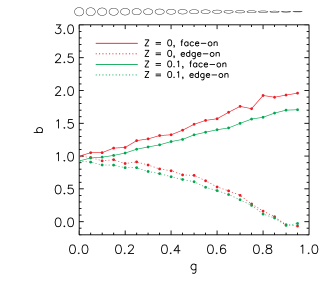
Figure 17.— EW “boost” $b$ when observing the system face-on (solid) and edge-on (dotted) as a function of flattening $g\equiv 1-c/a$, where $a$ and $c$ are the semi-major and -minor axes of the system (shown schematically as small ellipses in the top of the plot). Results are shown for both dust-free (red) and dusty (green, $Z=0.1\mbox{$Z_{\odot}$}$) gas. In both cases the gas is homogeneous, and the column density is $N_{\textrm{{\scriptsize H}{\tiny\hskip 0.28453ptI}}}=2\times 10^{20}$ cm^-2, as measured along the $c$-axis. For reference, the Milky Way has a flatness of $g\sim 0.95$-0.99 (Binney & Merrifield, 1998).

This effect is of course observationally impracticable, except statistically, but has also been investigated in more realistic galaxy simulations. In Laursen et al. (2009b), Ly$\alpha$ RT was carried out in a sample of nine randomly oriented galaxies extracted from a fully cosmological simulation and resimulated at high resolution. The ratio of the fluxes escaping in the most luminous to the least luminous direction, roughly corresponding to what would be interpreted as an EW boost, was in the range 1.5–4 if integrating over the whole galaxy, and $\sim 10$ if looking at the region of maximum surface brightness only. From LABEL:flat, this corresponds roughly to “boosts” of 1.1–1.5 and $\sim 2$, respectively. Similar values was found by Zheng et al. (2010) (a ratio of seven for the central region of a single galaxy) and Barnes et al. (2011) (a ratio of 1.7–3 for various implementations of galactic winds). More recently, Yajima et al. (2012b) found no preferred direction of escape for a single, cosmologically simulated galaxy at $z=3.1$, but a strong dependence on viewing angle at $z=0$ when the galaxy had settled into a disk, similar to what was found by Verhamme et al. (2012) for an isolated disk galaxy.

6.1.6 Cooling radiation

At high redshifts, a large fraction of galaxies may be expected to be in the process of forming, i.e. to accrete gas from the surrounding medium, resulting in collisionally excited Hi leading to Ly$\alpha$ emission. Since the implied densities are rather high, the timescale for cooling is generally smaller than the dynamical timescale, and thus the infalling gas should be relatively cold ($T\sim 10^{4}$ K, e.g. Fall & Rees, 1985; Haiman & Rees, 2001). Consequently, roughly 50% of the energy is emitted in the Ly$\alpha$ line alone (Fardal et al., 2001).

For relatively massive galaxies, Goerdt et al. (2010) found at $z=2.5$ that cold gas accreting can give rise to significant Ly$\alpha$ emission of up to a few times $10^{-17}$ erg s^-1 cm^-2 arcsec^-2 on scales of 10-100 kpc, which is comparable to typical line strengths. Such gravitational cooling not only gives rise to Ly$\alpha$ radiation but also to a continuum, although relatively it is much fainter than the stellar continuum. Dijkstra (2009) calculated analytically the EW of the cooling radiation from a collapsing halo and found that, depending on where the continuum is measured, the intrinsic EW of the cooling radiation is $\gtrsim 950$ Å. Numerically, a few studies have addressed this issue and find that in general the fraction of the Ly$\alpha$ radiation that stems from gravitational cooling increases with $z$, from $\sim 10$% at $z=3.6$ (Laursen & Sommer-Larsen, 2007), to $\sim 16$-18% at $z=5.7$–6.5 (Dayal et al., 2010), to $\sim 50$-60% at $z=7$–8 (Jensen et al., 2012). Similarly, Yajima et al. (2012a) found that cooling radiation becomes comparable to recombination Ly$\alpha$ for $z>6$. Obviously, large deviations from these values exist, both numerically and in reality, as in the case of Ly$\alpha$ blobs where in some cases no stellar continuum is seen at all; a liable explanation for these objects is cold accretion (Nilsson et al., 2006; Dijkstra & Loeb, 2009)

However, while the photons of stellar origin, both Ly$\alpha$ and continuum, tend to be born in regions of comparatively high densities of both dust and neutral gas, thus being more prone to dust absorption, the cooling photons may escape more or less freely. Thus, cooling radiation could dominate even at quite low redshifts, although the actual fraction is difficult to assess observationally as long as the escape fraction of stellarly produced photons is still associated with so large uncertainties.

6.1.7 IGM extinction

At high redshifts, neutral hydrogen in the IGM scatter a significant fraction of the photons blueward of the Ly$\alpha$ line out of the line of sight. This affects both the continuum and the line itself, and is sometimes accounted for using a model of the IGM absorption. For instance, Malhotra & Rhoads (2002) use the prescription of Madau (1995) and found that the corrections for the broadband and the narrowband approximately cancel, leaving the EW unaffected. This assumes that the Ly$\alpha$ line is symmetric about the line center; if the red peak is enhanced relative to the blue peak, as would be the case for an expanding medium, the IGM transmits more Ly$\alpha$, resulting in the erroneous interpretation that the EW is larger than in reality. Moreover, as the galaxies detected in Ly$\alpha$ at high redshifts may be biased toward being the ones that have made themselves visible by ionizing a bubble around them in an otherwise partly neutral IGM, the line may be less affected by the IGM than the continuum, which again would be interpreted as an EW boost.

Even if the correlation of the state of the IGM with the sources is taken into account, large fluctuations in the neutral fraction of hydrogen exists, which may also be a possible source of error (e.g. Laursen et al., 2011; Jeeson-Daniel et al., 2012). Using a simple model for LAEs at high redshifts but incorporating clumpiness of the IGM, Hayes et al. (2006) calculate distribution functions for observed EWs, for various narrowband/broadband techniques. They found that, depending on the redshift, the median $W_{\mathrm{obs}}$ may easily lie appreciatively above $W_{\mathrm{em}}$, and that for instance at $z=5.7$ with narrowband and broadband both centered on the Ly$\alpha$ line, 20% of the EWs will be boosted by a factor of 2 or higher.

6.1.8 Star formation stochasticity

When calculating the resulting EW from a distribution of stellar masses, an infinite number of stars are usually assumed. Using the numerical code SLUG (Fumagalli et al., 2011; da Silva et al., 2012), Forero-Romero & Dijkstra (2012) found that for low-SFRs galaxies, stochasticity alone results in a distribution of EWs from $W_{0}/4$ to $3W_{0}$, where $W_{0}$ is the mean EW. However, since this effect is minimal for SFRs $\gtrsim 1$ $M_{\odot}$ yr^-1, which are hardly visible at high redshifts, it cannot serve as an explanation for most of the observed high-EW galaxies.

6.1.9 Inhomogeneous escape

For resolved galaxies, regions with no star formation may scatter Ly$\alpha$ from distant regions toward the observer, such that these particular regions exhibit extreme EWs (Hayes et al., 2007). Integrated over the source, however, Ly$\alpha$-overluminous regions cancel out with underluminous regions (modulo other effects affecting the RT).

7. Summary and conclusion

We have carried out a comprehensive set of Ly$\alpha$ and FUV continuum radiative transfer calculations, systematically varying the significant physical parameters, first separately and then in unison. The aim was to investigate whether a multiphase interstellar medium is capable of preferentially absorbing the continuum so as to enhance the observed Ly$\alpha$ equivalent width. The motivation for this study are the numerous observations of Ly$\alpha$ emitting galaxies exhibiting EWs larger than what is theoretically expected, together with the previously proposed explanation of such a “boost” being a consequence of a clumpy ISM (Neufeld, 1991; Hansen & Oh, 2006). In the suggested model, a galaxy consists of a number of clouds, physically corresponding to the ISM phase termed the “warm neutral medium”, dispersed in a low-density medium corresponding to the phase called the “hot ionized medium”.

We find that, while indeed it is possible to construct a model galaxy with the said ability, the physical properties needed are extremely unlikely to be found in a real galaxy. In order for a galaxy to enhance its intrinsic Ly$\alpha$ EW, a large number of criteria must be met:

1. The metallicity must be high ($\gtrsim$ Solar),

2. the density of the WNM must be very high ($\gtrsim 5$ times typical values),

3. the density of the HIM and its ionization fraction must be very low, so that the total density of neutral hydrogen in this phase does not exceed $\sim 10^{-7}$ cm^-3,

4. the bulk ($>80$–90%) of the Ly$\alpha$ and FUV photons must originate from regions where the stars have blown away the neutral gas from which they were born,

5. the galaxy must have virtually no outflows ($\mbox{$V_{\mathrm{out}}$}\lesssim 10$ ${\rm km\,s^{-1}}$), and

6. the velocity dispersion of the gas clouds must be very low ($\lesssim 10$ ${\rm km\,s^{-1}}$).

In particular the latter two points are important; the whole point of the proposed multiphase model is that the paths of the Ly$\alpha$ photons are confined to a dust- and gasless medium, never penetrating the dusty clouds but instead scattering off of their surfaces. This mechanism works because of the resonance nature of Ly$\alpha$ scattering. However, as soon as the clouds have a small velocity, especially random motions, the Ly$\alpha$ photons are shifted out of resonance in the reference frame of the clouds, allowing them to penetrate much farther into the clouds and thus exposing them to a higher column density of dust. Note that in principle it is possible to have an enhanced EW for larger velocity fields, but this will require even more extreme conditions regarding the other parameters. With regards to the required densities of neutral hydrogen, these are more characteristic of the so-called cold neutral medium or molecular clouds. Since the volume occupied by these phases are much smaller than that of the WNM (e.g. Ferrière, 2001), the covering factor of these phases is small. Moreover, they will typically be embedded inside the WNM, affecting only those photons that were already trapped in the clouds. In addition to the points mentioned above, it must also be remembered that the intrinsic Ly$\alpha$ EW of a galaxy exhibiting a high observed EW must be high, i.e. the stellar population must be very young ($\sim$a few Myr); otherwise an even higher boost would be needed to bring the EW above the theoretical limit.

In conclusion, we consider the Neufeld model to be an extremely unlikely reason for the observed high EWs. We have discussed a number of other possible explanation (Sec. 6.1), of which the most probable, in our opinion, is excess of Ly$\alpha$ radiation from cold accretion (may contribute $\sim 0.1$–1 times the stellar Ly$\alpha$, depending on redshift, but may escape much more easily), and/or anisotropic escape of Ly$\alpha$ (the Ly$\alpha$ flux may vary in different directions by a factor $\sim 1$–10, depending on irregularity of the galaxy and aperture of the detector.

Appendix A Extending and testing MoCaLaTA

A.1. Implementing continuum radiation

The original version of MoCaLaTA included only the RT of Ly$\alpha$, i.e. the initial frequency probability distribution of photons followed a Voigt profile with the Gaussian core given by the temperature/turbulence of the gas. To calculate EWs, the wavelength range $\Delta\lambda$ transferred though the medium must be extended so as to include the continuum. For a given EW this is readily accomplished by first determining whether an emitted photon is a line rather than a continuum photon, with a probability $P(\textrm{line})\propto W_{\mathrm{int}}/\Delta\lambda$, and then determining the exact wavelength of the photon depending on the intrinsic line profile or the slope of the continuum (in this study taken to be flat in $\nu$). For a broad wavelength region around Ly$\alpha$, numerically there is no difference in the RT of the two kinds of photons.

A.2. Building the grid

In order to construct spherical clouds, we make use of adaptive mesh refinement (AMR), where cells may be refined into eight subcells. As the clouds themselves are uniform, high resolution is only needed at their surfaces, not their interior. To build the AMR grid, we use the following approach:

Given a number $N_{\mathrm{cl}}$ of clouds and a distribution of sizes specified by a minimum and maximum radius $r_{\mathrm{min}}$ and $r_{\mathrm{max}}$, as well as a size distribution power law index $\beta$, cloud centers are placed randomly in a sphere of radius $r_{\mathrm{gal}}$, such that no clouds overlap. The clouds’ surfaces are then marked by a number of auxiliary particles, typically $\sim 10^{3}$. Subsequently, the grid is constructed starting from a mother grid of base resolution $2^{3}$, recursively refining any cell that contains more than one particle. Finally, each cell is labeled either a “cloud” cell or an “ICM” cell, depending on the distance to the nearest cloud center, and the physical parameters then assigned accordingly. Note that all cells belonging to a given cloud share the same bulk velocity, such that there are no velocity gradients inside a cloud.

The auxiliary particles can be positioned in different ways so as to constitute the cloud surface; the most straightforward way is to place them at a random position at a distance $r_{\mathrm{cl}}$ from the center of the cloud. However, it turns out that in general some particles end up so close to each other, that in order to refine the cells sufficiently, hundreds of refinement levels may needed. Distributing the particles evenly on the surface ensures that roughly the same level of refinement is needed everywhere. Various algorithms exist for this geometrical exercise (see, e.g., Saff & Kuijlaars, 1997).

A.3. Altering the acceleration scheme

To speed up calculations, MoCaLaTA makes use of various acceleration schemes. The most efficient is the core-skipping scheme: Since scatterings of photons near the line center are usually associated with negligible spatial movement, while it typically takes of the order $10^{5}$ scatterings to “escape” the core, these scatterings can be skipped by drawing the random velocity of the scattering atom from a centrally-truncated Gaussian, favoring fast moving atoms that can give the photon a large Doppler shift. In MoCaLaTA, the critical wavelength defining when the acceleration scheme can be invoked is dependent on the product $a\tau_{0}$, such that for higher Hi column densities and lower temperatures, a larger critical value can be used, allowing for a larger speed-up. The value of $a\tau_{0}$ is specific to a given cell, and is calculated from the center of the cell to the face.

Since the code has previously been used for galaxies extracted from cosmological simulations, cells are usually surrounded by other cells of similar physical conditions, i.e. there are no large gradients. In the present, idealized simulations, however, where densities may go from zero to some extreme value over the course of a single cell step, this poses a problem for photons close to the line center scattering on the surface of a cloud.

In reality, the photon typically escapes after a handful of scatterings, changing its frequency only of the order 1.5 Doppler widths. With the acceleration scheme, the first scattering pushes the photon artificially far out in the wing, rendering the optical depth of hydrogen significantly reduced, such that the photon is able to penetrate the cloud (or the next cloud) too much, with a corresponding higher probability of being absorbed by dust.

We solve this issue by calculating $a\tau_{0}$ not from the cell center, but from the current position of the photon to the face of the cell. Unfortunately, the consequence is a quite less efficient acceleration.

A.4. Testing the code

In the original Neufeld scenario, that is with no velocity fields etc., the physical parameters most important to the RT are $N_{0}$ and $\epsilon_{\mathrm{c}}$, i.e. the average number of clouds with which a Ly$\alpha$ photon emitted from the center of a spherical conglomeration of clouds interacts, and the probability per cloud interaction that a photon (Ly$\alpha$ or continuum) is absorbed. No analytical solution exist for these quantities, but HO06 found that they could be well fitted by $N_{0}=\mbox{$f_{\mathrm{c}}$}^{2}+\frac{4}{5}\mbox{$f_{\mathrm{c}}$}$ (in the absence of absorption) and $\epsilon_{\mathrm{c}}\simeq 3\epsilon_{i}^{5/9}/(1+2\epsilon_{i}^{1/2})$, where $\epsilon_{i}$ is the probability of absorption per $[$gas or dust$]$ interaction for an incident photon lying at $x_{i}$ Doppler widths from the line center. The results are shown in LABEL:test.

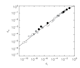
Figure 18.— Left panel: Average number $N_{0}$ of clouds with which a Ly$\alpha$ photon interacts before escaping from the center of a spherical multiphase medium, as a function of the covering factor $f_{\mathrm{c}}$ of clouds. Error bars indicate the region within which 68% of the photons fall. Right panel: Probability of being absorbed rather than reflected from the surface of a dusty cloud after numerous scatterings, as a function of probability of absorption in a single $[$gas or dust$]$ interaction event for a photon at an incident frequency $x_{i}$ Doppler widths from the line center. Each shade correspond to different values of dust cross section: From lightest to darkest 0.01, 0.1, 1, and 10 $\times 10^{-21}$ cm². For each value, seven different incident photon frequencies $x_{i}$ were run: From left to right, $x_{i}=20,10,5,4,2,1$, and 0. In both panels, the solid line shows the fits found by HO06.

References

- Atek et al. (2008) Atek, H., Kunth, D., Hayes, M., Östlin, G., & Mas-Hesse, J. M. 2008, A&A, 488, 491
- Barnes et al. (2011) Barnes, L. A., Haehnelt, M. G., Tescari, E., & Viel, M. 2011, MNRAS, 416, 1723
- Battinelli & Capuzzo-Dolcetta (1991) Battinelli, P., & Capuzzo-Dolcetta, R. 1991, MNRAS, 249, 76
- Bertone et al. (2005) Bertone, S., Stoehr, F., & White, S. D. M. 2005, MNRAS, 359, 1201
- Bershady et al. (2011) Bershady, M. A., Martinsson, T. P. K., Verheijen, M. A. W., Westfall, K. B., Andersen, D. R., & Swaters, R. A. 2011, ApJ, 739, L47
- Binney & Merrifield (1998) Binney, J., & Merrifield, M. 1998, Galactic astronomy, Princeton University Press, Princeton, NJ
- Binney & Tremaine (2008) Binney, J., & Tremaine, S. 2008, Galactic Dynamics, 2nd ed., Princeton University Press, Princeton, NJ
- Blanc et al. (2011) Blanc, G. A., Adams, J. J., Gebhardt, K., et al. 2011, ApJ, 736, 31
- Bridge et al. (2012) Bridge, C. R, et al. 2012, arXiv:1205.4030
- Brinks et al. (2000) Brinks, E., Walter, F., & Kerp, J. 2000, Revista Mexicana de Astronomía y Astrofísica Conference Series, 9, 279
- Bromm et al. (2001) Bromm, V., Kudritzki, R. P., & Loeb, A. 2001, ApJ, 552, 464
- Carilli et al. (1998) Carilli, C. L., Dwarakanath, K. S., & Goss, W. M. 1998, ApJ, 502, L79
- Chapman et al. (2005) Chapman, S. C., Blain, A. W., Smail, I., & Ivison, R. J. 2005, ApJ, 622, 772
- Charlot & Fall (1993) Charlot, S., & Fall, S. M. 1993, ApJ, 415, 580
- Christensen et al. (2012a) Christensen, L., Laursen, P., Richard, J., Hjorth, J., Milvang-Jensen, B., Dessauges-Zavadsky, M., Limousin, M., Grillo, C., & Ebeling, H. 2012a, arXiv:1209.0775
- Christensen et al. (2012b) Christensen, L., Richard, J., Hjorth, J., Laursen, P., Dessauges-Zavadsky, M., Grillo, C., & Ebeling, H. 2012b, arXiv:1209.0767
- Churchwell (1990) Churchwell, E. 1990, A&A Rev., 2, 79
- da Silva et al. (2012) da Silva R. L., Fumagalli M., & Krumholz M., 2012, ApJ, 745, 145
- Dawson et al. (2007) Dawson, S., Rhoads, J. E., Malhotra, S., et al. 2007, ApJ, 671, 1227
- Dawson et al. (2004) Dawson, S. et al. 2004, ApJ, 617, 707
- Dayal et al. (2008) Dayal, P., Ferrara, A., & Gallerani, S. 2008, MNRAS, 389, 1683
- Dayal et al. (2010) Dayal, P., Ferrara, A., & Saro, A. 2010, MNRAS, 402, 1449
- Dayal et al. (2009) Dayal, P., Ferrara, A., Saro, A., et al. 2009, MNRAS, 400, 2000
- Dayal et al. (2011) Dayal, P., Maselli, A., & Ferrara, A. 2011, MNRAS, 410, 830
- de Avillez & Breitschwerdt (2005) de Avillez, M. A., & Breitschwerdt, D. 2005, A&A, 436, 585
- Dickey & Garwood (1989) Dickey, J. M., & Garwood, R. W. 1989, ApJ, 341, 201
- Dijkstra (2009) Dijkstra, M. 2009, ApJ, 690, 82
- Dijkstra et al. (2006a) Dijkstra, M., Haiman, Z., & Spaans, M. 2006, ApJ, 649, 14
- Dijkstra et al. (2006b) Dijkstra, M., Haiman, Z., & Spaans, M. 2006, ApJ, 649, 37
- Dijkstra & Kramer (2012) Dijkstra, M., & Kramer, R. 2012, MNRAS, 424, 1672
- Dijkstra & Loeb (2009) Dijkstra, M. & Loeb, A. 2009, MNRAS, 396, 377
- Dijkstra & Wyithe (2010) Dijkstra, M., & Wyithe, J. S. B. 2010, MNRAS, 408, 352
- Dopita & Sutherland (2003) Dopita, M. A., & Sutherland, R. S. 2003, Astrophysics of the diffuse universe, Berlin, New York: Springer, 2003. Astronomy and astrophysics library, ISBN 3540433627,
- Duval et al. (2012) Duval, F., Schaerer, D., Östlin, G, & Laursen, P. 2012, …
- Elmegreen & Clemens (1985) Elmegreen, B. G., & Clemens, C. 1985, ApJ, 294, 523
- Epinat et al. (2009) Epinat, B., Contini, T., Le Fèvre, O., Vergani, D., Garilli, B., Amram, P., Queyrel, J., Tasca, L., & Tresse, L. 2009, A&A, 504, 789
- Fall & Rees (1985) Fall, S. M., & Rees, M. J. 1985, ApJ, 298, 18
- Fardal et al. (2001) Fardal, M. A., Katz, N., Gardner, J. P., Hernquist, L., Weinberg, D. H., & Davé, R. 2001, ApJ, 562, 605
- Ferrière (2001) Ferrière, K. M. 2001, Reviews of Modern Physics, 73, 1031
- Field et al. (1969) Field, G. B., Goldsmith, D. W., & Habing, H. J. 1969, ApJ, 155, L149
- Finkelstein et al. (2009a) Finkelstein, S. L., Cohen, S. H., Malhotra, S., & Rhoads, J. E. 2009a, ApJ, 700, 276
- Finkelstein et al. (2011a) Finkelstein, S. L., Cohen, S. H., Moustakas, J., et al. 2011a, ApJ, 733, 117
- Finkelstein et al. (2011b) Finkelstein, S. L., Cohen, S. H., Windhorst, R. A., et al. 2011b, ApJ, 735, 5
- Finkelstein et al. (2009b) Finkelstein, S. L., Malhotra, S., Rhoads, J. E., Hathi, N. P., & Pirzkal, N. 2009b, MNRAS, 393, 1174
- Finkelstein et al. (2009c) Finkelstein, S. L., Rhoads, J. E., Malhotra, S., & Grogin, N. 2009c, ApJ, 691, 465
- Finkelstein et al. (2008) Finkelstein, S. L., Rhoads, J. E., Malhotra, S., Grogin, N., & Wang, J. 2008, ApJ, 678, 655
- Finkelstein et al. (2007) Finkelstein, S. L., Rhoads, J. E., Malhotra, S., Pirzkal, N., & Wang, J. 2007, ApJ, 660, 1023
- Fosbury et al. (2003) Fosbury, R. A. E. et al. 2003, ApJ, 596, 797
- Forero-Romero & Dijkstra (2012) Forero-Romero, J. E., & Dijkstra, M. 2012, arXiv:1206.0726
- Franco (2012) Franco, G. A. P. 2012, A&A, 543, A39
- Fruchter et al. (2006) Fruchter, A. S., et al. 2006, Nature, 441, 463
- Fumagalli et al. (2011) Fumagalli, M., da Silva, R. L., & Krumholz, M. R., 2011, ApJ, 741, L26
- Fynbo et al. (2003) Fynbo, J. P. U., Ledoux, C., Møller, P., Thomsen, B. & Burud, I. 2003, A&A, 407, 147
- Förster Schreiber et al. (2009) Förster Schreiber, N. M. et al. 2009, ApJ, 706, 1364
- Gaensler et al. (2011) Gaensler, B. M., Haverkorn, M., Burkhart, B., Newton-McGee, K. J., Ekers, R. D., Lazarian, A., McClure-Griffiths, N. M., Robishaw, T., Dickey, J. M., Green, A. J. 2011, Nature, 478, 214
- Gall et al. (2011) Gall, C., Andersen, A. C., & Hjorth, J. 2011, A&A, 528, A13
- Garay & Lizano (1999) Garay, G., & Lizano, S. 1999, PASP, 111, 1049
- Garel et al. (2012) Garel, T., Blaizot, J., Guiderdoni, B., Schaerer, D., Verhamme, A., & Hayes, M. 2012, MNRAS, 422, 310
- Gawiser et al. (2006) Gawiser, E., et al. 2006, ApJ, 642, L13
- Gawiser et al. (2007) Gawiser, E., et al. 2007, ApJ, 671, 278
- Gendelev & Krumholz (2012) Gendelev, L., & Krumholz, M. R. 2012, ApJ, 745, 158
- Giavalisco et al. (1996) Giavalisco, M., Koratkar, A., & Calzetti, D. 1996, ApJ, 466, 831
- Gloeckler & Geiss (2004) Gloeckler, G., & Geiss, J. 2004, Advances in Space Research, 34, 53
- Goerdt et al. (2010) Goerdt, T., Dekel, A., Sternberg, A., Ceverino, D., Teyssier, R., & Primack, J. R. 2010 MNRAS, 407, 613
- Gouliermis et al. (2012) Gouliermis, D. A., Schmeja, S., Dolphin, A. E., Gennaro, M., Tognelli, E., Prada Moroni, P. G. 2012, ApJ, 748, 64
- Gronwall et al. (2007) Gronwall, C. et al. 2007, ApJ, 667, 79
- Grove et al. (2009) Grove, L. F., Fynbo, J. P. U., Ledoux, C., Limousin, M., Møller, P., Nilsson, K. K., & Thomsen, B. 2009, A&A, 497, 689
- Haiman & Rees (2001) Haiman, Z. & Rees, M. 2001, ApJ, 556, 87
- Hansen & Oh (2006) Hansen, M. & Oh, S. P. 2006, MNRAS, 367, 979
- Hashimoto et al. (2012) Hashimoto, T., Ouchi, M., Shimasaku, K., Ono, Y., Nakajima, K., Rauch, M., Lee, J., Okamura, S. 2012, arXiv:1206.2316
- Hayes et al. (2006) Hayes, M., & Östlin, G. 2006, A&A, 460, 681
- Hayes et al. (2007) Hayes, M., Östlin, G., Atek, H., Kunth, D., Mas-Hesse, J. M., Leitherer, C., Jiménez-Bailón, E., & Adamo, A. 2007, MNRAS, 382, 1465
- Hayes et al. (2010) Hayes, M., Östlin, G., Schaerer, D., Mas-Hesse, J. M., Leitherer, C., Atek, H., Kunth, D., Verhamme, A., de Barros, S., & Melinder, J. 2010, Nature, 464, 562
- Heckman (2002) Heckman, T. M. 2002, ASPC, 254, 292
- Heiles & Troland (2003) Heiles, C., & Troland, T. H. 2003, ApJ, 586, 1067
- Henry et al. (2010) Henry, A. L., Martin, C. L., Dressler, A., McCarthy, P., & Sawicki, M. 2010, ApJ, 719, 685
- Herrera-Camus et al. (2012) Herrera-Camus, R., Fisher, D. B., Bolatto, A. D., Leroy, A. K., Walter, F., Gordon, K. D., Roman-Duval, J., Donaldson, J., Meléndez, M., Cannon, J. M. 2012, ApJ, 752, 112
- Hosokawa & Inutsuka (2006) Hosokawa, T., & Inutsuka, S.-i. 2006, ApJ, 646, 240
- Hosokawa et al. (2011) Hosokawa, T., Omukai, K., Yoshida, N., & Yorke, H. W. 2011, Science, 334, 1250
- House (1964) House, L. L. 1964, ApJS, 8, 307
- Hu & McMahon (1996) Hu, E. M., & McMahon, R. G. 1996, Nature, 382, 231
- Hu et al. (2004) Hu, E.M., Cowie, L. L., Capak, P., McMahon, R. G., Hayashino, T., & Komiyama, Y. 2004, AJ, 127, 563
- Ianjamasimanana et al. (2012) Ianjamasimanana, R., de Blok, W. J. G., Walter, F., & Heald, G. H. 2012, arXiv:1207.5041
- Imara et al. (2011) Imara, N., Bigiel, F., & Blitz, L. 2011, ApJ, 732, 79
- Inoue (2003) Inoue, A. K. 2003, PASJ, 55, 901
- Israel (1978) Israel, F. P. 1978, A&A, 70, 769
- Jeeson-Daniel et al. (2012) Jeeson-Daniel, A., Ciardi, B., Maio, U., et al. 2012, MNRAS, 424, 2193
- Jensen et al. (2012) Jensen, H., Laursen, P., Mellema, G., Iliev, I. T., Sommer-Larsen, J., & Shapiro, P. R. 2012, arXiv:1206.4028
- Johnson & Axford (1971) Johnson, H. E., & Axford, W. I. 1971, ApJ, 165, 381
- Kashikawa et al. (2006) Kashikawa, N., et al. 2006, ApJ, 648, 7
- Kashikawa et al. (2011) Kashikawa, N., et al. 2011, ApJ, 734, 119
- Kashikawa et al. (2012) Kashikawa, N., et al. 2012, arXiv:1210.4933
- Kim et al. (2003) Kim, S., Staveley-Smith, L., Dopita, M. A., Sault, R. J., Freeman, K. C., Lee, Y., Chu, Y.-H. 2003, ApJS, 148, 473
- Knude (1979) Knude, J. 1979, A&A, 71, 344
- Knude (1981) Knude, J. 1981, A&A, 97, 380
- Kobayashi et al. (2010) Kobayashi, M. A. R., Totani, T., & Nagashima, M. 2010, ApJ, 708, 1119
- Kudritzki et al. (2000) Kudritzki, R.-P., Méndez, R. H., Feldmeier, J. J., Ciardullo, R., Jacoby, G. H., Freeman, K. C., Arnaboldi, M., Capaccioli, M., Gerhard, O., & Ford, H. C. 2000, ApJ, 536, 19
- Kulas et al. (2012) Kulas, K. R., Shapley, A. E., Kollmeier, J. A., Zheng, Z., Steidel, C. C., & Hainline, K. N. 2012, ApJ, 745, 33
- Kunth et al. (1998) Kunth, D., Mas-Hesse, J. M., Terlevich, E., Terlevich, R., Lequeux, J., & Fall, S. M. 1998, A&A, 334, 11
- Lada & Lada (2003) Lada, C. J., & Lada, E. A. 2003, ARA&A, 41, 57
- Lai et al. (2007) Lai, K., Huang, J., Fazio, G., Cowie, L. L., Hu, E. M., & Kakazu, Y. 2007, ApJ, 655, 704
- Laursen et al. (2009a) Laursen, P., Razoumov, A. O., & Sommer-Larsen, J. 2009, ApJ, 696, 853
- Laursen & Sommer-Larsen (2007) Laursen, P. & Sommer-Larsen, J. 2007, ApJ, 657, L69
- Laursen et al. (2011) Laursen, P., Sommer-Larsen, J., & Razoumov, A. O. 2011, ApJ, 728, 52
- Laursen et al. (2009b) Laursen, P., Sommer-Larsen, J., & Andersen, A. C. 2009b, ApJ, 704, 1640
- Madau (1995) Madau, P. 1995, ApJ, 441, 18
- Mattsson (2011) Mattsson, L 2011, MNRAS, 414, 781
- McElroy (1995) McElroy, D. B. 1995, ApJS, 100, 105
- McKee & Ostriker (1977) McKee, C. F. & Ostriker, J. P. 1977, ApJ, 218, 148
- Malhotra & Rhoads (2002) Malhotra, S. & Rhoads, J. E. 2002, ApJ, 565, L71
- Malhotra & Rhoads (2004) Malhotra, S. & Rhoads, J. E. 2004, ApJ, 617, L5
- Malhotra et al. (2012) Malhotra, S., Rhoads, J. E., Finkelstein, S. L., Hathi, N., Nilsson, K., McLinden, E., & Pirzkal, N. 2012, ApJ, 750, L36
- Mallery et al. (2012) Mallery, R. P., et al. 2012, arXiv:1208.6031
- Nakajima et al. (2012) Nakajima, K., Ouchi, M., Shimasaku, K., et al. 2012, ApJ, 745, 12
- Neufeld (1991) Neufeld, D. 1991, ApJ, 370, L85
- Newton (1980) Newton, K. 1980, MNRAS, 191, 615
- Niino et al. (2009) Niino, Y., Totani, T., & Kobayashi, M. A. R. 2009, ApJ, 707, 1634
- Nilsson et al. (2006) Nilsson, K. K., Fynbo, J. P. U., Møller, P., Sommer-Larsen, J. & Ledoux, C. 2006, A&A, 452, 23
- Nilsson et al. (2007) Nilsson, K. K., Møller, P., Möller, O., Fynbo, J. P. U., Michalowski, M. J., Watson, D., Ledoux, C., Rosati, P., Pedersen, K., Grove, L. F. 2007, A&A, 471, 71
- Nilsson et al. (2009) Nilsson, K. K., Tapken, C., Møller, P., Freudling, W., Fynbo, J. P. U., Meisenheimer, K., Laursen, P., Östlin, G. 2009, A&A, 498, 13
- Nilsson et al. (2010) Nilsson, K. K., Östlin, G., Møller, P., Møller-Nilsson, O., Tapken, C., Freudling, W., & Fynbo, J. P. U. 2011, A&A, 529, A9
- Noterdaeme et al. (2012) Noterdaeme, P., Laursen, P., Petitjean, P., Vergani, S. D., Maureira, M. J., Ledoux, C., Fynbo, J. P. U., López, S., & Srianand, R. 2012, A&A, 540, A63
- Orsi et al. (2012) Orsi, A., Lacey, C. G., & Baugh, C. M. 2012, MNRAS, 425, 87
- Ouchi et al. (2005) Ouchi, M. et al. 2005, ApJ, 620, 1
- Ouchi et al. (2008) Ouchi, M. et al. 2008 ApJS, 176, 301
- Paladini et al. (2012) Paladini, R. et al. 2012, arXiv:1210.3631
- Park et al. (2009) Park, S.-J., Min, K.-W., Seon, K.-I., Han, W., Lee, D.-H., Edelstein, J., Korpela, E., & Sankrit, R. 2009, ApJ, 700, 155
- Pentericci et al. (2009) Pentericci, L., Grazian, A., Fontana, A., Castellano, M., Giallongo, E., Salimbeni, S., & Santini, P. 2009, A&A, 494, 553
- Peterson & Caldwell (1993) Peterson, R. C. & Caldwell, N. 1993, AJ, 105, 1411
- Pettini et al. (1997) Pettini, M., King, D., Smith, L., & Hunstead, R. 1997, ApJ, 478, 536
- Pettini et al. (2001) Pettini, M., Shapley, A. E., Steidel, C. C., Cuby, J., Dickinson, M., Moorwood, A. F. M., Adelberger, K. L., & Giavalisco, M. 2001, ApJ, 554, 981
- Pirzkal et al. (2007) Pirzkal, N., Malhotra, S., Rhoads, J. E., & Xu, C. 2007, ApJ, 667, 49
- Prochaska et al. (2006) Prochaska, J. X., O’Meara, J. M., Herbert-Fort, S., Burles, Scott, Prochter, Gabriel E., & Bernstein, Rebecca A. 2006, ApJ, 648, L97
- Quider et al. (2009) Quider, A. M., Pettini, M., Shapley, A. E., & Steidel, C. C. 2009, MNRAS, 398, 1263
- Raiter et al. (2010) Raiter, A., Schaerer, D., & Fosbury, R. A. E. 2010, A&A, 523, A64
- Rhoads et al. (2003) Rhoads, J. E., Dey, A., Malhotra, S., et al. 2003, AJ, 125, 1006
- Richling et al. (2003) Richling, S. 2003, MNRAS, 344, 553
- Roy et al. (2010) Roy, I., Shu, C.-W., & Fang, L.-Z. 2010, ApJ, 716, 604
- Rubin et al. (2011) Rubin, K. H. R., Prochaska, J. X., Ménard, B., Murray, N., Kasen, D., Koo, D. C., & Phillips, A. C. 2011, ApJ, 728, 55
- Rupke et al. (2002) Rupke, D. S., Veilleux, S., & Sanders, D. B. 2002, ApJ, 570, 588
- Saff & Kuijlaars (1997) Saff, E. B., & Kuijlaars, A. B. J. 1997, Mathematical Intelligencer, 19.1, 5
- Salpeter (1955) Salpeter, E. 1955, ApJ, 121, 161
- Savaglio et al. (2003) Savaglio, S., Fall, M. S. & Fiore, F. 2003, ApJ, 585, 638
- Savaglio et al. (2012) Savaglio, S. et al. 2012, MNRAS, 420, 627
- Schaerer (2002) Schaerer, D. 2002, A&A, 382, 28
- Schaerer (2003) Schaerer, D. 2003, A&A, 397, 527
- Schönrich et al. (2010) Schönrich, R., Binney, J., & Dehnen, W. 2010, MNRAS, 403, 1829
- Shapley et al. (2003) Shapley, A. E., Steidel, C. C., Pettini, M., & Adelberger, K. L. 2003, ApJ, 588, 65
- Shimasaku et al. (2006) Shimasaku, K., et al. 2006, PASJ, 58, 313
- Skillman et al. (1987) Skillman, E. D., Bothun, G. D., Murray, M. A., & Warmels, R. H. 1987, A&A, 185, 61
- Stark et al. (2010) Stark, D. P., Ellis, R. S., Chiu, K., Ouchi, M., & Bunker, A. 2010, MNRAS, 408, 1628
- Steidel et al. (2010) Steidel, C. C., Erb, D. K., Shapley, A. E., Pettini, M., Reddy, N., Bogosavljević, M., Rudie, G. C., & Rakic, O. 2010, ApJ, 717, 289
- Šurlan et al. (2012) Šurlan, B., Hamann, W.-R., Kubát, J., Oskinova, L. M., & Feldmeier, A. 2012, A&A, 541, A37
- Sutherland & Dopita (1993) Sutherland, R. S., & Dopita, M. A. 1993, ApJS, 88, 253
- Swinbank et al. (2011) Swinbank, A. M., Papadopoulos, P. P., Cox, P., Krips, M., Ivison, R. J., Smail, I., Thomson, A. P., Neri, R., Richard, J., & Ebeling, H. 2011, ApJ, 742, 11
- Tapken et al. (2007) Tapken, C., Appenzeller, I., Noll, S., Richling, S., Heidt, J., Meinköhn, E., Mehlert, D. 2007, A&A, 467, 63
- Thomas et al. (2012) Thomas, D. et al. 2012, arXiv:1207.6115
- Tüllmann et al. (2008) Tüllmann, R., Gaetz, T. J., Plucinsky, P. P., Long, K. S., Hughes, J. P., Blair, W. P., Winkler, P. F., Pannuti, T. G., Breitschwerdt, D., Ghavamian, P. 2008, ApJ, 685, 919
- Tüllmann et al. (2006) Tüllmann, R., Pietsch, W., Rossa, J., Breitschwerdt, D., & Dettmar, R.-J. 2006, A&A, 448, 43
- Tumlinson & Shull (2000) Tumlinson, J., & Shull, J. M. 2000, ApJ, 528, L65
- Tumlinson et al. (2003) Tumlinson, J., Shull, J. M., & Venkatesan, A. 2003, ApJ, 584, 608
- Valls-Gabaud (1993) Valls-Gabaud, D. 1993, ApJ, 419, 7
- van Zee et al. (1997) van Zee, L., Haynes, M. P., Salzer, J. J., & Broeils, A. H. 1997, AJ, 113, 1618
- van Zee et al. (1998) van Zee, L., Westpfahl, D, Haynes, M. P., & Salzer, J. J. 1998, ApJ, 115, 1000
- Veilleux et al. (2005) Veilleux, S., Cecil, G., & Bland-Hawthorn, J. 2005, ARA&A, 43, 769
- Venemans et al. (2005) Venemans, B., et al. 2005, A&A, 431, 793
- Verhamme et al. (2012) Verhamme, A., Dubois, Y., Blaizot, J., Garel, T., Bacon, R., Devriendt, J., Guiderdoni, B., & Slyz, A. 2012, arXiv:1208.4781
- Verhamme et al. (2008) Verhamme, A., Schaerer, D., Atek, H., & Tapken, C. 2008, A&A, 491, 89
- Verhamme et al. (2006) Verhamme, A., Schaerer, D., & Maselli, A. 2006, A&A, 460, 397
- Acquaviva et al. (2012) Acquaviva, V., Vargas, C., Gawiser, E., & Guaita, L. 2012, ApJ, 751, L26
- Waller et al. (1987) Waller, W. H., Clemens, D. P., Sanders, D. B., & Scoville, N. Z. 1987, ApJ, 314, 397
- Wang et al. (2004) Wang, J. X., Rhoads, J. E., Malhotra, S.,Dawson, S., Stern, D., Dey, A., Heckman, T. M., Norman, C. A., & Spinrad, H. 2004, ApJ, 608, L21
- Williams & McKee (1997) Williams, J. P., & McKee, C. F. 1997, ApJ, 476, 166
- Wolfire et al. (2003) Wolfire, M. G., McKee, C. F., Hollenbach, D., & Tielens, A. G. G. M. 2003, ApJ, 587, 278
- Xu et al. (2011) Xu, W., Wu, X.-P., & Fang, L.-Z. 2011, MNRAS, 418, 853
- Yajima et al. (2012c) Yajima, H., & Li, Y. 2012, arXiv:1211.0088
- Yajima et al. (2012a) Yajima, H., Li, Y., Zhu, Q., & Abel, T. 2012, MNRAS, 424, 884
- Yajima et al. (2012b) Yajima, H., Li, Y., Zhu, Q., Abel, T., Gronwall, C., & Ciardullo, R. 2012, ApJ, 754, 118
- Yamada et al. (2012) Yamada, T., Matsuda, Y., Kousai, K., Hayashino, T., Morimoto, N. & Umemura, M. 2012, arXiv:1203.3633
- Yang et al. (1994) Yang, H., Skillman, E. D., & Sramek, R. A. 1994, AJ, 107, 651
- Yuma et al. (2010) Yuma, S., Ohta, K., Yabe, K., et al. 2010, ApJ, 720, 1016
- Zackrisson et al. (2011) Zackrisson, E., Inoue, A. K., Rydberg, C.-E., & Duval, F. 2011, MNRAS, 418, L104
- Zheng et al. (2010) Zheng, Z., Cen, R., Trac, H., & Miralda-Escudé, J. 2010, ApJ, 716, 574
- Östlin et al. (2009) Östlin, G., Hayes, M., Kunth, D., Mas-Hesse, J. M., Leitherer, C., Petrosian, A., Atek, H. 2009, ApJ, 138, 923