On the Habitable Zones of Circumbinary Planetary Systems

Abstract

The effect of the stellar flux on exoplanetary systems is becoming an increasingly important property as more planets are discovered in the Habitable Zone (HZ). The Kepler mission has recently uncovered circumbinary planets with relatively complex HZs due to the combined flux from the binary host stars. Here we derive HZ boundaries for circumbinary systems and show their dependence on the stellar masses, separation, and time while accounting for binary orbital motion and the orbit of the planet. We include stability regimes for planetary orbits in binary systems with respect to the HZ. These methods are applied to several of the known circumbinary planetary systems such as Kepler-16, 34, 35, and 47. We also quantitatively show the circumstances under which single-star approximations break down for HZ calculations.

1. Introduction

The Habitable Zone (HZ) is broadly defined as the region around a star where water can exist in a liquid state on the surface of a planet with sufficient atmospheric pressure. The boundaries of the HZ are usually calculated based upon the properties of the host star, with assumptions regarding the response of the planetary atmosphere to stellar flux. Attempts to quantify these boundaries have evolved considerably since initial discussions on the topic by Huang (1959, 1960). Hart (1979) provided estimates for the Solar System and later models of runaway greenhouse for Venus were incorporated into the calculations by Pollack (1971) and Kasting (1988). Kasting et al. (1993) calculated detailed one-dimensional (altitude) climate models and considered conditions whereby the equilibrium would sway to a runaway greenhouse effect or to a runaway snowball effect, thereby providing robust estimates of the HZ boundaries for main sequence stars.

Interestingly, much of the work on the HZ preceded the discovery of exoplanets. The exoplanet parameter-space, specifically orbital period and planetary mass, is slowly being expanded by different techniques. For example, the radial velocity (RV) technique has explored well beyond the HZ for main sequence stars, allowing analysis of HZ properties of these systems (Kane & Gelino, 2012a). Exoplanet systems tend to be dominated by Jovian planets, many of which are in highly eccentric orbits which causes the planet to pass through the HZ (Kane & Gelino, 2012b). There have also been several notable discoveries of super-Earths in the HZ, such as Gl 581d (Udry et al., 2007) and Gl 667Cc (Anglada-Escudé et al., 2012; Delfosse, 2012). The transit method is also contributing to the census of HZ planets. The Kepler mission is designed to explore the HZ (Kaltenegger & Sasselov, 2011) and has already found several which meet this criteria, such as Kepler-20b (Borucki et al., 2012).

One of the more interesting discoveries to result from the Kepler mission is that of circumbinary planets, or planets that orbit the center-of-mass of a central binary system. The first of these announced was Kepler-16b (Doyle et al., 2011), soon to be followed by Kepler-34b & Kepler-35b (Welsh et al., 2012), and the multi-planet system Kepler-47b,c (Orosz et al., 2012). There have been several discussions regarding the HZ for these systems, though these to-date approximate the calculations as a single-star for the purposes of determining the HZ boundaries (Quarles et al., 2012; Orosz et al., 2012).

Here we perform a more thorough analysis of the HZ boundaries for circumbinary planetary systems. We consider the contributions of both stars and the resulting position dependence of the HZ boundaries. We thus determine the mass/separation ratio dependence of these boundaries and include the orbital motion of the binary to produce a time dependent map of the HZ. We apply these calculations to the known Kepler circumbinary planetary systems of Kepler-16, 34, 35, and 47.

2. Habitable Zones of Single Star Systems

The HZ for single star systems defined by stellar irradiation has been discussed by a number of sources, most notably by Kasting et al. (1993). The boundaries of the HZ for main sequence stars have been further quantified as a function of effective temperature (Underwood et al., 2003; Selsis et al., 2007; Jones & Sleep, 2010). Note that there are additional influences on the habitability such as the effects of tides (Barnes et al., 2009; Heller et al., 2011) and orbital stability (Kopparapu & Barnes, 2010). Here we consider only the irradiation effects on the HZ and briefly describe the essential components which we expand upon in future sections.

One of the fundamental stellar properties which determines the extent of the HZ is the luminosity of the host star, which is approximated as

$$L_{\star}=4\pi R_{\star}^{2}\sigma T_{\mathrm{eff}}^{4}$$ (1)

where $\sigma$ is the Stefan-Boltzmann constant. The model adopted by Kasting et al. (1993) utilizes the principle of a planetary energy balance: net incoming solar radiation must equal the net outgoing infra-red (IR) radiation. This method determines the stellar flux, $S$, for which the outgoing IR radiation is sustainable for various atmospheric assumptions. The underlying implication here is that the stellar flux received at the HZ boundaries is dependent on the amount of IR radiation incident upon the upper atmosphere. Thus there is a temperature dependence on the host star. Using the boundary conditions of runaway greenhouse and maximum greenhouse effects at the inner and outer edges of the HZ respectively (Underwood et al., 2003), the stellar flux at these boundaries are given by

$$S_{\mathrm{inner}}=4.190\times 10^{-8}T_{\mathrm{eff}}^{2}-2.139\times 10^{-4}T_{\mathrm{eff}}+1.268$$ (2)

$$S_{\mathrm{outer}}=6.190\times 10^{-9}T_{\mathrm{eff}}^{2}-1.319\times 10^{-5}T_{\mathrm{eff}}+0.2341\ .$$ (3)

The inner and outer edges of the HZ are then derived from the following

$$r_{\mathrm{inner}}=\sqrt{L_{\star}/S_{\mathrm{inner}}}$$ (4)

$$r_{\mathrm{outer}}=\sqrt{L_{\star}/S_{\mathrm{outer}}}$$ (5)

where the radii are in units of AU and the stellar luminosities are in solar units. The dependence of these boundaries upon the wavelength of the incident radiation is of critical importance when considering two separate radiation sources.

3. Habitable Zones of Multi-Stellar Systems

In this section we generalize the above principles to multi-stellar systems. The HZ of planets in S-type orbits (planets orbiting one component of a stellar binary) has been considered in detail by Eggl et al. (2012) and applied to $\alpha$ Centauri B by Forgan (2012), now known to host a terrestrial exoplanet (Dumusque et al., 2012). We address the specific case of HZ boundaries for planets in P-type orbits, where the planet orbits the center of mass of both stars.

3.1. Combined Black-body Spectrum and Stellar Flux

The radiation received at any point in a binary system is a combination of two blackbody spectral radiances. First we consider Planck’s law as a function of wavelength, $\lambda$:

$$I(\lambda,T)=\frac{2hc^{2}}{\lambda^{5}}\frac{1}{e^{hc/\lambda kT}-1}$$ (6)

where $T$ is the effective temperature. Note that this equation is per steradian. The stellar flux received at a particular location may then be expressed by the following equations for star 1 and star 2:

$$S_{1}=\frac{2\pi hc^{2}}{\lambda^{5}}\frac{1}{e^{hc/\lambda kT_{\mathrm{eff},1}}-1}\left(\frac{R_{\star,1}}{r_{1}}\right)^{2}$$ (7)

$$S_{2}=\frac{2\pi hc^{2}}{\lambda^{5}}\frac{1}{e^{hc/\lambda kT_{\mathrm{eff},2}}-1}\left(\frac{R_{\star,2}}{r_{2}}\right)^{2}$$ (8)

where $R_{\star,1}$ and $R_{\star,2}$ are stellar radii and $r_{1}$ and $r_{2}$ are the distances from a given location to star 1 and star 2 respectively. The total flux received at this location is then $S=S_{1}+S_{2}$. Wien’s Displacement Law ($\lambda_{\mathrm{max}}T_{\mathrm{eff}}=2.9\times 10^{-3}$) may then be used to estimate the equivalent effective temperature of a single energy source that would produce the same energy flux. For the purposes of integrating the total flux over all wavelengths, Equations 7 and 8 reduce to the Stefan-Boltzmann law. However, it is important to consider the wavelength dependence of the incident flux, as we will see in later sections.

Figure 1.— The blackbody spectra of the individual stars in the binary system and the combined flux for both stars. The peak of the combined spectrum peaks at a wavelength of 528 nm (vertical line) which, using Wien’s Displacement Law, is equivalent to a temperature of 5481 K.

As an example, consider the case of a binary system consisting of a G2V star and a K5V star, separated by 0.1 AU. Shown in Figure 1 are the individual and combined blackbody spectra for this system. The total flux peaks at a wavelength of 528 nm which is equivalent to a temperature of 5481 K. This particular evaluation of the blackbody spectra does not take into account the distances to the stars. When the radii and distances are included, this introduces a spatial dependence.

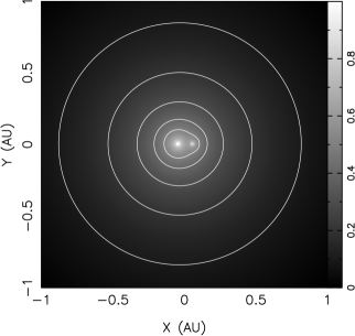
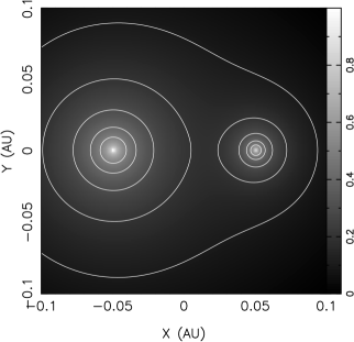
Figure 2.— The stellar flux map, depicted with both gray scale and contours, of a binary system consisting of a G2V and a K5V star with a separation of 0.1 AU. The right panel is a zoom of the left panel. In each panel, the calculated flux has been converted to a logarithmic scale and normalized to lie between 0 and 1. On this scale, the contours are equal to values of 0.1 to 0.5 in steps of 0.1 moving from the outer edge inwards.

Figure 2 shows a flux map of the same system with two different zoom levels to emphasize the contribution from both stars. For the purposes of contrast, the calculated flux has been converted to a logarithmic scale and normalized to lie between 0 and 1. On this flux scale, the contours are equal to values of 0.1 to 0.5 in steps of 0.1 moving from the outer edge inwards. There is a clear asymmetry associated with the presence of the second star which is particularly noticeable at distances closer than 0.3 AU.

3.2. Habitable Zone Boundaries

The traditional HZ due to stellar irradiance for a single star is calculated as a function of both the stellar flux received and the peak wavelength of the energy distribution. For a single star, this has a radial dependence in a spherical geometry which allows an analytical solution for the inner and outer HZ boundaries. For a multi-stellar system, the locations of these boundaries is far more complex, since both the stellar flux and peak wavelength have non-radial dependencies due to the combinational effect produced from the two stars at a particular location.

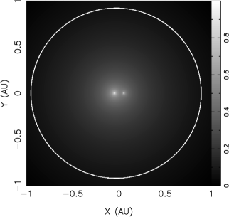
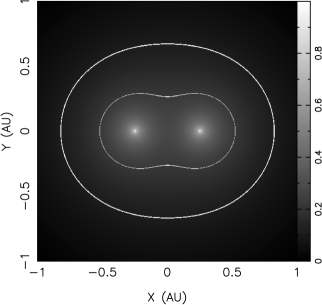
Figure 3.— The stellar flux map shown as a gray scale map (as for Figure 2) and the HZ boundaries for two different binary configurations. The left panel depicts these quantities for the G2V–K5V binary discussed in detail in Section 3.1 where only the inner edge of the HZ is shown on this scale. The right panel depicts these for an equal-mass binary consisting of two M0V stars separated by 0.5 AU. In this case both the inner and outer edge of the HZ are shown on the plot with a very clear asymmetry to those boundaries.

We approach this problem by constructing a two-dimensional grid in the orbital plane of the binary star. For each grid location we perform the following steps: (1) calculate the combined stellar flux, (2) calculate the combined blackbody function and determine the peak, (3) convert the wavelength for the peak into effective temperature using Wien’s Displacement Law, and (4) calculate the expected stellar flux at the HZ boundaries for this temperature using Equations 2 and 3. If the calculated stellar flux at that location matches that expected for a HZ boundary then that grid position is marked as such.

Figure 3 depicts the HZ boundaries for two example binaries: the G2V–K5V binary described in §3.1 with a separation of 0.1 AU (left panel), and an equal-mass binary consisting of two M0V stars separated by 0.5 AU (right panel). The inner HZ boundary for the G2V–K5V binary appears symmetric on this scale, but the distance of the boundary from the primary (G2V) star varies between 0.90 and 0.94 AU. For the secondary star, this distance ranges from 0.84 to 1.01 AU. The asymmetric HZ boundaries for the M0V–M0V binary shown in the right panel represents a far more extreme case where both the inner and outer boundaries are plotted.

Figure 4.— The dependence of the HZ asymmetry on the binary separation for the previously discussed cases of a G2V–K5V and M0V–M0V binary. At each separation, the axis ratio of both the inner and outer HZ boundaries are computed.

The asymmetry in the HZ boundaries may be quantified as a function of the binary separation by considering the axis ratio of both the inner and outer boundaries of the HZ. We performed a simulation of this dependence by calculating the HZ boundaries in the cases of the two examples described above. We utilized a range of separations between 0.01 and 1.0 AU and located the minimum and maximum values of both the inner and outer boundaries. The results of this simulation are shown in Figure 4. The case of the G2V–K5V shows moderate variation in the inner HZ asymmetry but negligible variation in the outer HZ. For the equal-mass M0V–M0V binary, the asymmetry rapidly increases with increasing separation for both the inner and outer boundaries.

3.3. The Keplerian Orbit of the Binary

The orbital elements of binary stars are known to encompass a broad range of orbital periods and mass ratios (see for example Halbwachs et al. (2005) and Mathieu et al. (2004)). This diversity results in an equally varying range of HZ structures due to the mass ratios and binary separations. From a fixed location relative to the binary center-of-mass, the apparent HZ boundaries will have a time dependence owing to the orbital motion of the binary.

For a Keplerian (non-circular) binary orbit, assuming a fixed reference point, the changing HZ boundaries will have an additional disparity resulting from the varying binary separation. This will result in an oscillating HZ structure as the binary rotates around their center-of-mass. As shown in the previous sections, the oscillation will have a much larger effect for low-mass stars than for solar-type stars. The large variation in flux within typical HZ regions may ultimately render some binary systems uninhabitable.

4. Planets Within the Habitable Zone

Now we consider a planetary orbit which is passing through asymmetric HZ regions and the flux/temperature variations that result.

4.1. Stable Configurations

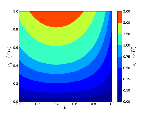
Figure 5.— A contour plot of the dependence of the critical semi-major axis of a planetary orbit, $a_{c}$, on the mass-ratio, $\mu$, and separation, $a_{b}$ of a binary star (Holman & Wiegert, 1999).

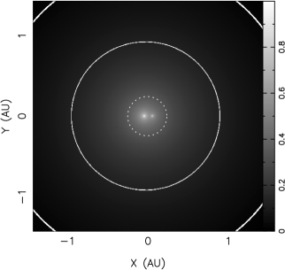
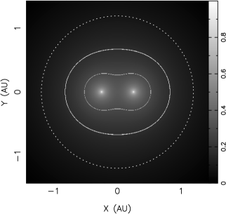
Figure 6.— The stellar flux map shown as a gray scale map and HZ boundaries (solid lines) for a G2V–K5V (left panel) and M0V–M0V (right panel) binary, as for Figure 3. Also shown in each case is the boundary for the critical semi-major axis (dotted line), beyond which planetary orbits may retain long-term stability. This shows that the stable planetary orbits may exist in the HZ for the G2V–K5V binary, but stable orbits are excluded for the HZ of the M0V–M0V binary.

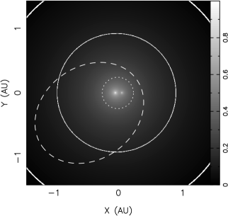
Figure 7.— Top panel: The G2V–K5V binary system showing the HZ boundaries (solid lines), critical semi-major boundary (dotted line), and a planetary orbit (dashed line). The planetary orbit has a semi-major axis of $a=0.9$ AU and an eccentricity of $e=0.6$. Bottom panel: The equilibrium temperature of the planet as a function of planetary orbital phase. Phase 0.0 is at apastron and phase 0.5 is at periastron.

Stable planetary orbits in both S-type and P-type systems have been discussed by a variety of authors, including Harrington (1977), but more recently by such authors as Eggleton & Kiseleva (1995) and Musielak et al. (2005). We adopt the formalism of Holman & Wiegert (1999) which provides analytical solutions for planetary orbital stability in binary star systems. For P-type orbits, this is a function of the binary separation, $a_{b}$, the mass ratio, $\mu$, and the eccentricity of the binary orbit. The mass ratio is defined as $\mu=m_{2}/(m_{1}+m_{2})$, such that an equal mass binary has a mass ratio of $\mu=0.5$. For a binary in a circular orbit, or $e=0$, Equation 3 of Holman & Wiegert (1999) may be expressed as

$$a_{c}=(1.60+4.12\mu-5.09\mu^{2})a_{b}$$ (9)

where $a_{c}$ is the minimum allowed semi-major axis of the planet. Figure 5 shows the dependence on $a_{b}$ and $\mu$ of the critical semi-major axis of a planet orbiting the center-of-mass of the binary. For binary separations of $a_{b}<0.2$ AU, the critical semi-major axis is only weakly dependent upon the mass ratio of the binary. As pointed out by Holman & Wiegert (1999), there often exists instability islands beyond $a_{c}$ which occur at mean-motion resonances. Thus the critical semi-major axis calculations here represent a lower limit on the total stability regions within a given system.

Applying this stability criteria to the two examples discussed thus far will yield whether or not a stable planetary orbit can be maintained within the HZ of those systems. Figure 6 is similar to Figure 3 in that it shows the stellar flux map and HZ boundaries for the G2V–K5V and M0V–M0V binaries, but slightly zoomed out so the outer part of the HZ for the G2V–K5V binary is visible. Also shown are dotted lines which indicate the critical semi-major axis for planets within the system, centered upon the binary center-of-mass in each case. This clearly shows that stable planetary orbits within the HZ for the G2V–K5V binary are possible but the the presence of planets are excluded from the HZ of the M0V–M0V binary.

4.2. The Keplerian Orbit of the Planet

A planet in orbit around the center-of-mass of the binary will experience variable conditions due to the rotation of the binary, as mentioned in §3.3. An additional component of the total flux variation is due to the Keplerian motion of the planetary orbit. The radial dependence of the flux means that the influence of the binary motion received at the planet will be more pronounced when the planet is passing through periastron passage.

As a demonstration, we include the presence of a planet in the G2V–K5V binary system example used throughout this paper (recall that our particular M0V–M0V binary example excludes stable orbits within the HZ for the binary separation used). We show the stellar flux map (see §3.1) in Figure 7, along with the HZ boundaries (see §3.2), the critical semi-major axis boundary (see §4.1), and the orbit of the planet. The planet has a semi-major axis of 0.9 AU and an eccentricity of 0.6 such that it spends most of the orbit within the HZ of the system. At each location of the orbit, we recalculate the flux received by the planet and estimate the equilibrium temperature of the planet assuming that the incident flux is redistributed around the entire planet (see Kane & Gelino (2011)). We also account for the stellar binary motion at each location during the planetary orbit. The bottom panel of Figure 7 shows the change in this temperature during one complete orbital phase as the planet moves from apastron (phase $=0.0$) to periastron (phase $=0.5$) and back again. The long-term variation is caused by the Keplerian orbit of the planet and the short-term variations are caused by the 9 day orbital period of the binary. The temperature variations can be dominated by either the orbits of the binary or the planet, depending on the relative orbital configurations.

4.3. Binary/Planet Dynamical Interactions

Thus far we have assumed a decoupling of the Keplarian motion of the binary and the Keplerian motion of the planet. However, the secular dynamical interactions in the system will result in a break-down of the periodic behaviour one may otherwise obtain when you assume the planet and binary are orbitally decoupled. Although the semi-major axis of the planet’s orbit will remain relatively unchanged, the shape (eccentricity) and orientation (argument of periastron) will have time-dependent components. This has been described in detail by various authors, including analytical solutions for stellar triples (Söderhjelm, 1984; Georgakarakos, 2009), single-star multi-planet systems (Lee & Peale, 2003), effects of general relativity (Eggleton & Kisseleva-Eggleton, 2006), and the dynamics and stability of planets in circumbinary orbits (Doolin & Blundell, 2011). The amplitude of these variations depends on numerous factors, such as the relative inclinations of the orbits (Farago & Laskar, 2010). Here we assume co-planar orbits, as is the case for the Kepler systems discussed in the following section.

The timescale of the secular dynamical interactions is largely dominated by the periastron precession of the planet which occurs on much shorter timescales than the precession of the binary. The simulations by Doolin & Blundell (2011) of test particles in circumbinary orbits show that the period of the periastron precession of an orbiting planet is related to the semi-major axis of the orbit, $a$, via the power-law $\propto a^{3.5}$. Therefore, one can expect to be able to measure the effects of periastron precession for systems similar to those described here over the course of years, with a complete periastron precession period in the range of several decades. Although we are primarily concerned with the HZ of the binary systems, the stability and secular dynamics of the planetary orbits in those systems is an effect that one should consider when predicting the percentage of the orbital phase within the HZ over long periods or time.

5. Application to Known Systems

Here we apply the HZ boundary methods to several of the circumbinary exoplanetary systems found via the Kepler mission.

5.1. Kepler-16

Kepler-16b was discovered by Doyle et al. (2011) and was the first circumbinary planet announced as a result of transit observations by the Kepler mission. The binary system consists of 0.7 and 0.2 $M_{\odot}$ components in a 41 day eccentric orbit. The binary pair are orbited by a 0.3 $M_{J}$ planet with an orbital period of 229 days. The system has been the subject of numerous follow-up studies, such as that carried out by Winn et al. (2011) which showed that the plane of the stellar orbit, the planetary orbit, and the primary’s rotation are all closely aligned. Radial velocity observations by Bender et al. (2012) allowed the dynamical determination of masses for both of the binary components.

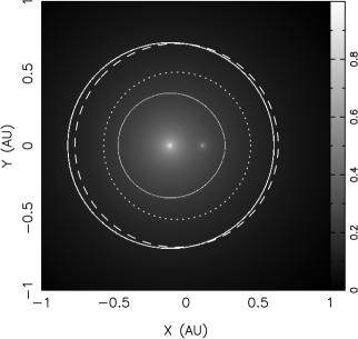
Figure 8.— Top panel: The Kepler-16 system showing the HZ boundaries (solid lines), critical semi-major boundary (dotted line), and planetary orbit (dashed line). Bottom panel: The equilibrium temperature of the planet as a function of planetary orbital phase. Phase 0.0 is at apastron and phase 0.5 is at periastron.

Figure 8 shows the flux map, HZ boundaries, critical semi-major axis (stability) boundary, and planetary orbit for Kepler-16. The effective temperature of the primary star, $T_{\mathrm{eff},1}=4450$ K, is provided by Doyle et al. (2011). For the secondary star, we adopt the temperature of the spectral template star proxy used by Bender et al. (2012), GJ 905, of $T_{\mathrm{eff},2}=2800$ K. Although there is a slight asymmetry in the inner HZ boundary, this is inside the stability boundary. Overall, the flux is clearly dominated by the primary star which produces an outer HZ boundary centered on the primary. Our simulation shows that the offset between the center-of-mass of the system and the flux distribution results in the orbit of the planet moving in and out of the HZ during one complete orbit. In other words, the asymmetry in the temperature variations experienced by the planet can occur even for circular orbits (see lower panel of Figure 8).

5.2. Kepler-34 & Kepler-35

Welsh et al. (2012) announced the discovery of two circumbinary planetary systems from the Kepler mission: Kepler-34 and Kepler-35. These systems are quite comparable in terms of the mass ratio and separation of the binary stars. Figures 9 and 10 show our calculations for the HZ conditions in both systems, respectively. The similarity of the stellar components in both cases yield analogous centroids for the HZ and stability boundaries, unlike the case of Kepler-16. The Kepler-34 binary consists of two near-solar components with $T_{\mathrm{eff},1}=5913$ K and $T_{\mathrm{eff},2}=5867$ K separated by 0.23 AU. Only the inner HZ boundary is shown since the combined flux of these stars pushes the outer boundary much farther out than for our own Solar System. The planet is in an eccentric orbit inside of the inner HZ boundary with a semi-major axis of 1.09 AU. The resulting planetary temperature variation has both clear short-term and long-term components.

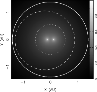
Figure 9.— Top panel: The Kepler-34 system showing the HZ boundaries (solid lines), critical semi-major boundary (dotted line), and planetary orbit (dashed line). Bottom panel: The equilibrium temperature of the planet as a function of planetary orbital phase. Phase 0.0 is at apastron and phase 0.5 is at periastron.

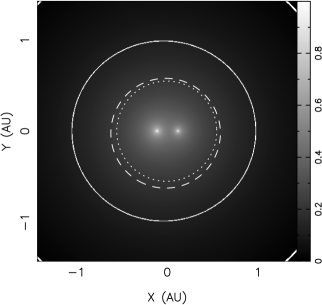
Figure 10.— Top panel: The Kepler-35 system showing the HZ boundaries (solid lines), critical semi-major boundary (dotted line), and planetary orbit (dashed line). Bottom panel: The equilibrium temperature of the planet as a function of planetary orbital phase. Phase 0.0 is at apastron and phase 0.5 is at periastron.

By comparison, the Kepler-35 system consists of stellar components with effective temperatures of 5606 K and 5202 K, respectively, separated by 0.18 AU. The HZ boundaries are thus smaller in size compared with Kepler-34. The planet’s near-circular orbit is very close to the stability boundary of the system, therefore the binary. This causes the temperature profile of the planet to be very sensitive to the orbital motion of the binary, as can be seen in the plot of the temperature variations during one complete orbital period.

5.3. Kepler-47

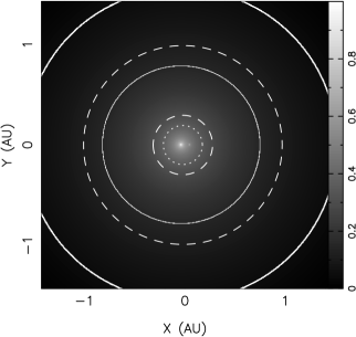
Figure 11.— Top panel: The Kepler-47 system showing the HZ boundaries (solid lines), critical semi-major boundary (dotted line), and orbits for the b and c planets (dashed lines). Middle panel: The equilibrium temperature of the b planet as a function of planetary orbital phase. Bottom panel: The equilibrium temperature of the c planet as a function of planetary orbital phase. Phase 0.0 is at apastron and phase 0.5 is at periastron.

The Kepler-47 system, discovered by Orosz et al. (2012), contains a binary star whose components are quite different, similar to Kepler-16. The two stars have temperatures of 5636 K and 3357 K, respectively, and are separated by only 0.08 AU. The resulting stellar flux dominated by the primary produces asymmetry in the flux only in the vicinity of the binary (within the stability boundary). The main difference between Kepler-47 the other studied Kepler systems, however, is that this system has two known transiting planets. Figure 11 shows our calculations for the Kepler-47 system, as well as the orbits and temperature profiles for the two planets. Both planets are in near-circular orbits with semi-major axes as 0.30 AU and 0.99 AU, respectively. As noted by Orosz et al. (2012), the outer planet resides within the HZ of the system throughout the entire orbit. Since the planets are in non-eccentric orbits, the temperature variations are dominated by the binary orbit, with an additional variation caused by the orbital center-of-mass offset from the primary stellar flux. The amplitude of the variations for the outer planet are relatively small, $\sim 5$ K, which is negligible for habitability considerations in this region.

6. Conclusions

Calculating the amount of time an exoplanet spends within the HZ around a circumbinary system is relatively complicated. First, we must consider the amount of stellar flux from both stars received by the exoplanet at any point in its orbit (§3.1). Then we must determine the wavelength at which this combined flux peaks and how that translates into an effective temperature (§3.1). This will then allow us to determine the inner and outer boundaries of the HZ (§3.2). Depending on the configuration of the binary masses and separation, the HZ boundaries may then experience a significant time-dependent orbital motion with respect to the rotation of the stars (§3.3). Finally, the stability of the binary system must be analyzed (§4.1) in order to fully understand the planetary orbit with respect to the oscillating HZ (§4.2).

We have applied our analysis to a number of known exoplanet-hosting binary systems (§5), namely Kepler-16, 34, 35, and 47. We have demonstrated that the circumstances under which a single-star approximation is viable is solely reliant on the stellar masses and separation of the binary. For example, the components in Kepler-16 and Kepler-47 are so dominated by the primary star that our analysis does not significantly change the approximation of the HZ as compared to a single-star model. However, the HZ in Kepler-16 is offset from the center of mass of the binary resulting in a planetary orbit that alternates in and out of the boundary. The binary stars within Kepler-34 and Kepler-35 are similar in mass and at such distances from each other that require our analysis to determine accurate HZs. The benefit of analyzing these Kepler systems, and Kepler systems in general, is that they exemplify the diversity we expect when exoplanets orbit binary systems.

To date, these circumbinary planetary systems are second only in complexity to the recently discovered double-binary system with an interposed exoplanet (Schwamb et al., 2012). In this instance, an exoplanet revolves around an eclipsing binary in a P-type configuration with a period of $\sim$ 138 days, while a second visual binary orbits at $\sim$ 1000 AU. The method that we have described here for determining the HZ boundaries could be applied to this quadruple system, as well as any system with an $n$-number of stars. The flux from the $n$-stars would need to be combined and the effective temperature determined. However, whether an exoplanet would be able to maintain a stable configuration within that system would be another matter. We anticipate further discoveries by the Kepler mission of new and interesting stellar and planetary configurations on which to apply our method.

References

- Anglada-Escudé et al. (2012) Anglada-Escudé, G., et al. 2012, ApJ, 751, L16
- Barnes et al. (2009) Barnes, R., Jackson, B., Greenberg, R., Raymond, S.N. 2009, ApJ, 700, L30
- Bender et al. (2012) Bender, C.F., et al. 2012, ApJ, 751, L31
- Borucki et al. (2012) Borucki, W.J., et al. 2012, ApJ, 745, 120
- Delfosse (2012) Delfosse, X., et al. 2012, A&A, submitted (arXiv:1202.2467)
- Doolin & Blundell (2011) Doolin, S., Blundell, K.M. 2011, MNRAS, 418, 2656
- Doyle et al. (2011) Doyle, L.R., et al. 2011, Science, 333, 1602
- Dumusque et al. (2012) Dumusque, X., et al. 2012, Nature, in press
- Eggl et al. (2012) Eggl, S., Pilat-Lohinger, E., Georgakarakos, N., Gyergyovits, M., Funk, B. 2012, ApJ, 752, 74
- Eggleton & Kiseleva (1995) Eggleton, P., Kiseleva, L. 1995, ApJ, 455, 640
- Eggleton & Kisseleva-Eggleton (2006) Eggleton, P., Kisseleva-Eggleton, L. 2006, Ap&SS, 304, 75
- Farago & Laskar (2010) Farago, F., Laskar, J. 2010, MNRAS, 401, 1189
- Forgan (2012) Forgan, D. 2012, MNRAS, 422, 1241
- Georgakarakos (2009) Georgakarakos, N. 2009, MNRAS, 392, 1253
- Halbwachs et al. (2005) Halbwachs, J.L., Mayor, M., Udry, S. 2005, A&A, 431, 1129
- Harrington (1977) Harrington, R.S. 1977, AJ, 82, 753
- Hart (1979) Hart, M.H. 1979, Icarus, 37, 351
- Heller et al. (2011) Heller, R., Leconte, J., Barnes, R. 2011, A&A, 528, 27
- Holman & Wiegert (1999) Holman, M.J., Wiegert, P.A. 1999, AJ, 117, 621
- Huang (1959) Huang, S.-S. 1959, PASP, 71, 421
- Huang (1960) Huang, S.-S. 1960, PASP, 72, 489
- Jones & Sleep (2010) Jones, B.W., Sleep, P.N., 2010, MNRAS, 407, 1259
- Kaltenegger & Sasselov (2011) Kaltenegger, L., Sasselov, D., 2011, ApJ, 736, L25
- Kane & Gelino (2011) Kane, S.R., Gelino, D.M. 2011, ApJ, 741, 52
- Kane & Gelino (2012a) Kane, S.R., Gelino, D.M. 2012, PASP, 124, 323
- Kane & Gelino (2012b) Kane, S.R., Gelino, D.M. 2012, Astrobiology, 12, 940
- Kasting (1988) Kasting, J.F. 1988, Icarus, 74, 472
- Kasting et al. (1993) Kasting, J.F., Whitmire, D.P., Reynolds, R.T. 1993, Icarus, 101, 108
- Kopparapu & Barnes (2010) Kopparapu, R.K., Barnes, R. 2010, ApJ, ApJ, 716, 1336
- Lee & Peale (2003) Lee, M.H., Peale, S.J. 2003, 592, 1201
- Mathieu et al. (2004) Mathieu, R.D., Meibom, S., Dolan, C.J. 2004, ApJ, 602, L121
- Musielak et al. (2005) Musielak, Z.E., Cuntz, M., Marshall, E.A., Stuit, T.D. 2005, A&A, 434, 355
- Orosz et al. (2012) Orosz, J.A., et al. 2012, Science, in press (arXiv:1208.5489)
- Pollack (1971) Pollack, J.B. 1971, Icarus, 14, 295
- Quarles et al. (2012) Quarles, B., Musielak, Z.E., Cuntz, M. 2012, ApJ, 750, 14
- Schwamb et al. (2012) Schwamb, M.E., et al. 2012, ApJ, submitted (arXiv:1210.3612)
- Selsis et al. (2007) Selsis, F., Kasting, J.F., Levrard, B., Paillet, J., Ribas, I., Delfosse, X., 2007, A&A, 476, 1373
- Söderhjelm (1984) Söderhjelm, S. 1984, A&A, 141, 232
- Udry et al. (2007) Udry, S., et al. 2007, A&A, 469, L43
- Underwood et al. (2003) Underwood, D.R., Jones, B.W., Sleep, P.N., 2003, Int. J. Astrobiology, 2, 289
- Welsh et al. (2012) Welsh, W.F., et al. 2012, Nature, 481, 475
- Winn et al. (2011) Winn, J.N., et al. 2011, ApJ, 741, L1