BPS states and their reductions

Abstract

We develop a method to identify the BPS states in the Hilbert space of a supersymmetric field theory on a generic curved space which preserves at least two real supercharges. We also propose a one-to-one map between BPS states in $d$-dimensional field theories and states that contribute to the supersymmetric partition function of a corresponding $(d-1)$-dimensional field theory. As an application we obtain the superconformal index on rounded and squashed three spheres, and we show a natural reduction of the respective indices to the three-dimensional exact partition functions. We discuss the validity of the correspondence both at the perturbative and at the non-perturbative level and exploit the idea to uplift the computation of the exact supersymmetric partition function on a general manifold to a higher dimensional index.

1 Introduction

Supersymmetric field theories on curved backgrounds are of great interest due to the fact that they capture the full quantum information about quantities of the corresponding field theory defined on flat space, where the same exact quantum results would be difficult to find.

Different choices of the background manifold correspond to a different information about the flat space theory. One of the first examples has been $T^{3}\times\mathbb{R}$ Witten:1982df , where the supersymmetric partition function counts supersymmetric vacua and has been dubbed index (see also Cecotti:1981fu ). Because it is an integer number, it cannot depend upon the continuous superpotential and gauge couplings, under mild assumptions. More recently another manifold, the Euclidean $S^{3}\times S^{1}$, has attracted much attention, because in this case the supersymmetric partition function is an index that counts a reduced set of states of the flat space theory, namely the BPS states Romelsberger:2005eg ; Kinney:2005ej . The latter are protected by supersymmetry so that a weak coupling computation can be continued to strong coupling and compared in the AdS/CFT framework to the computation of the graviton index in AdS space. The matching of the two indices on the two sides corroborates the conjectured duality between them. This is only one of the calculable exact results. By using localization Witten:1988hf , we can in principle compute the supersymmetric partition function (see Pestun:2007rz ) on any manifold that preserves at least one complex supercharge (or, in Euclidean space, two real supercharges), by reducing it to a matrix model, i.e. a finite dimensional ordinary integral.

Turning back to the case of the four-dimensional index, there are many available methods to obtain the matrix model formula for it. In Sen:1985dc ; Sen:1985ph ; Romelsberger:2005eg the BPS states on the sphere have been found explicitly from the knowledge of the spectrum of the Laplace operator: one needs to find the eigenmodes of the Laplace and Dirac operator on the sphere and sum over all the modes. Many of the bosonic modes will cancel out against the fermionic ones, and one finds that only the BPS modes contribute to the index. This is the most direct method, but it is in practice very difficult to work out on generic supersymmetry preserving manifolds. Another method is to compute the letter index Kinney:2005ej for theories defined on a conformally flat background. In these cases, it is straightforward to obtain the quantum numbers of the curved space fields because conformal mapping relates them to their flat space counterpart. We can then identify the operators that saturate the BPS inequality. Nevertheless it is not simple to extend this method to backgrounds that are not conformally flat. Finally, one can consider using localization. This amounts to picking a Q-exact term, generically related to the supersymmetry transformations, and evaluate the ratio of two determinants, which represents the full quantum corrections to the quantity one is considering .

Because of the difficulties of applying the previous methods to other manifolds, it is simpler to identify just the BPS states in the Hilbert space. One of the purposes of this paper is to develop a method to achieve this aim. The essential logic relies on the fact that the non-BPS modes are paired up by supersymmetry and hence the BPS modes correspond to the kernel of the boson-fermion map. The problem boils down to a set of first order differential equations.

We also argue a general relation between the BPS states and the set of states that contribute non trivially to a corresponding partition function in one dimension less. More precisely, we will see that there exists a one-to-one map between these two sets of states, and we identify the energy of each BPS state with the quantum contribution of the dimensionally reduced state to the supersymmetric partition function. This relation has two immediate consequences. The first one is that an index in $d$ dimensions reduces to a supersymmetric partition function for the dimensionally reduced field theory, thus providing an argument which generalizes previous observations for the three-sphere Dolan:2011rp ; Gadde:2011ia ; Imamura:2011uw .

Another consequence is the following. Since the states contributing to the partition function are the BPS states in one higher dimension, we can uplift the quantum contribution to the partition function to the computation of the energies of BPS states in one higher dimension and use the method outlined above. In this way, we only need to know the uplifted supersymmetry transformations and read from them the pairing map. We believe that this leads to a simplification in the computation of exact partition functions.

The paper is organized as follows. In section 2 we review the definitions for the quantities we are interested in, and explain our method to identify the BPS states in a general field theory. We also describe in full detail the relation between $d$-dimensional BPS states and the $(d-1)$-dimensional physical states, focusing on the $4d/3d$ case for concreteness. In section 3 we show how the computations can be worked out for the examples of the round and squashed spheres. We give all the necessary details to explicitly perform the computation, review previous results and discuss the physical meaning of our results applied to the cases at hand. The reduction of these two indices to the corresponding three-dimensional partition functions is shown in section 4. In section 5 we discuss generalizations of our technique to compute the index to other manifolds and dimensions, while the idea to uplift the computation of the partition function to a higher dimensional index is developed in section 6.

2 A correspondence between $4d$ and $3d$ states

One of the aims of the present paper is to develop a method to identify the BPS states and to compute the supersymmetric index and the partition function on a general class of manifolds. In doing that, we will point out a connection between these two objects in different dimensions. To be concrete, in this section we focus on the $4d/3d$ case.

Given a three-dimensional manifold ${\cal M}_{3}$ that preserves some supersymmetry, and given a four dimensional supersymmetric theory defined on $X\equiv{\cal M}_{3}\times S^{1}$, we can define two different quantities. The first one is the four dimensional superconformal index, defined on $X$, that only takes contributions from BPS states. It is the supersymmetric partition function

$${\cal I}_{sp}\left(t,y_{i}\right)={\rm Tr}(-)^{F}\,e^{-\tau\Xi}\,t^{H}\prod_{i}y_{i}^{\gamma_{i}}$$ (1)

where $\Xi\equiv\{Q,Q^{\dagger}\}$, $F$ is the fermion number and the trace is taken over every state in the theory. $H$ and the $\gamma$’s form a complete set of operators that commute with the conserved supercharge $Q$. In the following, we will call $H$ the energy operator and its eigenvalues the energies of the corresponding eigenstates. Moreover, the time direction is identified with the circle and is thus periodic with period $\tau$. The statement that the quantity (1) only takes contributions from BPS states means that for each bosonic state with $\Xi\neq 0$ there exists a fermionic state with the same $(\Xi,H,\gamma_{i})$ quantum numbers; thus, the index turns out to be independent of $\tau$ due to the boson-fermion cancellations, and the trace can be taken over the Hilbert space of $\Xi=0$ states. The index in (1) is the single particle index. In the case of a gauge theory one has to sum over all the possible gauge invariant configurations.

On the other hand, we can reduce the given supersymmetric theory on ${\cal M}_{3}$ itself and compute, at least in principle, the exact partition function for this theory via localization. The latter reduces the partition function to the matrix integral

$$Z_{{\cal M}_{3}}\sim\int\!\!{\rm[d\sigma]}\,\,e^{-S_{\ast}}\frac{{\rm Pf}{D_{F}}}{\sqrt{\det{D_{B}}}}$$ (2)

where $[$d$\sigma]$ represents the measure over the Cartan of the gauge group. We have set the following notation for the two quantities we are interested in. We denote by $S_{\ast}$ the classical action evaluated at the saddle points, while the exact quantum contribution from the generic superfield $\Phi$ is

$$Z_{\Phi}=\frac{{\rm Pf}{D_{F}}}{\sqrt{\det{D_{B}}}}$$ (3)

where $D_{F}$ and $D_{B}$ are, respectively, a linear first order and second order differential operator, and $\Phi$ labels both the chiral and gauge multiplets. A boson-fermion cancellation manifests itself in the fact that some of the eigenvalues simplify between the numerator and the denominator in (3).

We argue that the BPS states that contribute to (1) are in one-to-one correspondence to the states contributing to (3). More precisely, for each four-dimensional BPS state with eigenvalue $E$ of $H$ there is a three-dimensional state for which $E$ is an eigenvalue of the $D_{B}$ or of $D_{F}$ in the case of boson or fermion respectively.

These states can be found by solving a first order differential equation that can be directly read from the supersymmetry transformations of the four dimensional theory. Finally, the saddle points in (2) correspond to the zero energy states in the BPS spectrum: it follows that, if there is no zero energy solution for a four-dimensional field $\Phi$, the only three-dimensional saddle point corresponds to $\Phi=0$. We will give more details on this point in section 4.

An argument for this correspondence is the following. It is well known that the index (1) does not depend on the radius of the compact time direction and thus it does not change even when we shrink the circle to zero size. More precisely, consider a fermionic state $\psi$ of a four-dimensional theory and define a corresponding bosonic state

$$\phi\equiv\zeta\psi$$ (4)

where $\zeta$ is the Killing spinor which commutes with the BPS condition. Then $\phi$ has the same $(\Xi,H,\gamma_{i})$ quantum numbers and will cancel the contribution of $\psi$ in (1), unless $\phi=0$ or, equivalently, $\psi=\zeta F$, with $F$ a scalar function with the same $(\Xi,H,\gamma_{i})$ quantum numbers of $\psi$. If $\psi$ is a state of the theory it satisfies the corresponding equation of motion: if we set $\psi\sim\psi_{3}(\vec{x})e^{Et}$, it is thus easy to recognize that the four-dimensional equation of motion can be interpreted as the eigenvalue equation for a three-dimensional fermion with eigenvalue $E$.

We now consider the bosonic states that contribute to the index: we set up a map from the bosonic spectrum to the fermionic one by

$$\psi=i\sigma^{\mu}\tilde{\zeta}D_{\mu}\phi$$ (5)

which is an infinitesimal supersymmetry transformation (see below and section 3.1). We see that every boson that contributes to the index is given by $\sigma^{\mu}\tilde{\zeta}D_{\mu}\phi=0$. Once again, this can be interpreted as an eigenvalue equation for a three-dimensional bosonic mode that contributes non trivially to the partition function.

The argument above can be cast in the following form. In four dimensions, the supersymmetry transformations for the chiral multiplet are

$$\begin{split}\delta\phi&=\zeta\psi\\ \delta\psi&=\zeta F+i\sigma^{\mu}\tilde{\zeta}\,D_{\mu}\phi\\ \delta F&=\tilde{\zeta}\tilde{\sigma}^{\mu}{\cal D}_{\mu}\psi\end{split}$$ (6)

where our conventions are explained in section 3.1. Notice that the fermion equation of motion implies $\delta F=0$. This is a necessary condition that must be satisfied by the fermionic degrees of freedom.

The map that identifies the BPS states can be found to be

$$\begin{array}[]{rl}\text{fermion:}&\quad\psi=\zeta F\quad\text{and}\quad\tilde{\sigma}^{\mu}{\cal D}_{\mu}\psi=0\\ \text{boson:}&\quad i\sigma^{\mu}\tilde{\zeta}\,D_{\mu}\phi=0\\ \end{array}$$ (9)

We further notice the following. The system (9) implies $|\delta\psi|^{2}=0$ (in the absence of F-terms), and when the fields are independent on the time direction, we can dimensionally reduce the latter equation which becomes the three-dimensional saddle point equation used in the localization setting.

We now turn to the vector multiplet. Once again we can set up a map between the bosonic and the fermionic Hilbert space by using the supersymmetry transformations. Analogously to the discussion above, all the contributions will cancel out but those coming from the zero modes of the map.

In four dimensions, the physical fields in the vector multiplet are a gauge field $v_{\mu}$ and the gaugino $\lambda$. The supersymmetry transformations are

$$\begin{split}\delta v_{\mu}&=i\zeta\sigma_{\mu}\tilde{\lambda}-i\tilde{\zeta}\tilde{\sigma}_{\mu}\lambda\\ \delta\lambda&=\zeta D+i\sigma^{\mu\nu}F_{\mu\nu}\zeta\\ \delta D&=i\tilde{\zeta}\tilde{\sigma}^{\mu}{\cal D}_{\mu}\lambda-i\zeta\sigma^{\mu}{\cal D}_{\mu}\tilde{\lambda}\end{split}$$ (10)

The map that identifies BPS states can be found to be

$$\begin{array}[]{rl}\text{gaugino:}&~{}~{}~{}-i\tilde{\zeta}\tilde{\sigma}_{\mu}\lambda=\partial_{\mu}\varphi\quad\text{and}\quad i\tilde{\sigma}^{\mu}{\cal D}_{\mu}\lambda=0\\ \text{gauge boson:}&~{}~{}~{}i\sigma^{\mu\nu}F_{\mu\nu}\zeta=0\\ \end{array}$$ (13)

where once again $\delta D=0$ is a necessary condition for the gaugino degrees of freedom.

In the first line we had set the gauge field to a pure gauge configuration because any such solution does not give rise to a state in the Hilbert space of the theory and hence the gaugino does not have a superpartner state. Alternatively, we could have considered the map between the field strength $F_{\mu\nu}$ and the gaugino, which leads to the same condition. It is easy to see that the zero energy solutions to (10) reduce to the three-dimensional saddle point equations for a three-dimensional Q-exact action. The set of non-trivial solutions for $\lambda$ and $F_{\mu\nu}$ gives the Hilbert space we have to trace over in equation (1), or alternatively the spectrum of eigenvalues contributing to (3).

To summarize, we are led to the conclusion that a priori different exact results in different dimensions are related one to the other. The reduction of the four-dimensional index to the three-dimensional partition function follows directly from the proposed connection between the four-dimensional and three-dimensional states. While we will give more details on this point in section 4, we stress here that our claim is stronger than the dimensional reduction of the superconformal index to the partition function, because we set up a one-to-one map between states and eigenvalues of different operators.

On the one hand we look for eigenstates of the four-dimensional Hamiltonian, on the other hand we look for eigenstates of the equations of motion derived from a Q-exact three-dimensional Lagrangian, that contributes to the partition function. While the former is a first order differential operator, the latter is in general a second order one.

In the next section we will explicitly check our proposal in two cases: ${\cal M}_{3}=S^{3}$, in which case we can compare with known results, and ${\cal M}_{3}=S^{3}_{b}$, with $S^{3}_{b}$ a squashed sphere. In the latter case, because the index is a topological invariant, it can be cast in the same form as the index on a sphere via a redefinition of its arguments. However, we show that one can keep the original definitions and define a natural limit to recover the three-dimensional partition function on the squashed three-sphere computed in Hama:2011ea . We thus conclude that, although the index does not carry different physical information on different but topologically equivalent manifolds, it contains different information when we reduce the four-dimensional theory to a three-dimensional one by shrinking the time circle. It thus becomes interesting, from a three-dimensional point of view, to compute the four-dimensional index even on topologically equivalent manifolds.

3 Examples: sphere and squashed spheres

3.1 Review of rigid supersymmetry on a curved manifold

We review here a simple and recent procedure to place an $\mathcal{N}=1$ supersymmetric theory on a curved four-dimensional manifold Festuccia:2011ws . The basic idea is to start with $\mathcal{N}=1$ supergravity and take an appropriate limit such as to decouple gravity but preserve the classical background configuration. Because a convenient off-shell formulation and its couplings to matter fields are known, the gravitino supersymmetry transformation looks very simple Sohnius:1981tp ; Sohnius:1982fw

$$\begin{split}\delta\psi_{\mu}&=-2{\cal D}_{\mu}\zeta-2iV^{\nu}\sigma_{\mu\nu}\zeta\\ \delta\tilde{\psi}_{\mu}&=-2{\cal D}_{\mu}\tilde{\zeta}+2iV^{\nu}\tilde{\sigma}_{\mu\nu}\tilde{\zeta}\\ D_{\mu}&\equiv\nabla_{\mu}-iq_{A}A_{\mu}\\ {\cal D}_{\mu}&\equiv D_{\mu}-iq_{V}V_{\mu}\end{split}$$ (14)

where $q_{A}$ and $q_{V}$ are the charges ( under the $A$ and $V$ background gauge fields) of the field on which the covariant derivative is acting on. For the Killing spinor $\zeta$, $q_{A}^{\zeta}=1$ and $q_{V}^{\zeta}=-1$, and $\tilde{\zeta}$ has opposite quantum numbers. Because gravity is decoupled, one can give an expectation value to the background gauge fields $A$ and $V$ and to the metric without having to take care of their equations of motion.

Once we have found a solution to $\delta\psi_{\mu}=0$ and $\delta\tilde{\psi}_{\mu}=0$, the supersymmetry transformations of the matter fields are

$$\begin{split}\begin{array}[]{lll}\delta\phi=\zeta\psi&\qquad q_{A}^{\phi}=q&\qquad q_{V}^{\phi}=-1/2\\ \delta\psi=\zeta F+i\sigma^{\mu}\tilde{\zeta}\,D_{\mu}\phi&\qquad q_{A}^{\psi}=q-1&\qquad q_{V}^{\psi}=1/2\\ \delta F=\tilde{\zeta}\tilde{\sigma}^{\mu}{\cal D}_{\mu}\psi&\qquad q_{A}^{F}=q-2&\qquad q_{V}^{F}=3/2\end{array}\end{split}$$ (15)

for the chiral multiplet, and, in the Wess-Zumino gauge,

$$\begin{split}\begin{array}[]{lll}\delta v_{\mu}=i\zeta\sigma_{\mu}\tilde{\lambda}-i\tilde{\zeta}\tilde{\sigma}_{\mu}\lambda&\qquad q_{A}^{v}=0&\qquad q_{V}^{v}=-1/2\\ \delta\lambda=\zeta D+i\sigma^{\mu\nu}F_{\mu\nu}\zeta&\qquad q_{A}^{\lambda}=1&\qquad q_{V}^{\lambda}=-3/2\\ \delta D=i\tilde{\zeta}\tilde{\sigma}^{\mu}{\cal D}_{\mu}\lambda-i\zeta\sigma^{\mu}{\cal D}_{\mu}\tilde{\lambda}&\qquad q_{A}^{D}=0&\qquad q_{V}^{D}=-1/2\end{array}\end{split}$$ (16)

for the vector multiplet. An action which is invariant under these supersymmetry transformations is

$${\cal L} = {\cal L}^{B}+{\cal L}^{F}$$ (17)

$$\frac{{\cal L}^{B}}{\sqrt{g}} = \left(-\frac{1}{4}{\cal R}-\frac{3}{2}V_{\mu}V^{\mu}\right)q\phi\bar{\phi}-D_{\mu}\phi D^{\mu}{\bar{\phi}}+F\bar{F}$$

$$+{iV^{\mu}}\left(\bar{\phi}D_{\mu}\phi-\phi D_{\mu}\bar{\phi}\right)+\frac{1}{4}F_{\mu\nu}F^{\mu\nu}+\frac{1}{2}D^{2}$$

$$\frac{{\cal L}^{F}}{\sqrt{g}} = -{i}\tilde{\lambda}\tilde{\sigma}^{\mu}{\cal D}_{\mu}\lambda-{i}\tilde{\psi}\tilde{\sigma}^{\mu}{\cal D}_{\mu}\psi$$

3.2 Supersymmetry on a general squashed sphere

In this section we present all the necessary results to work out the examples of the sphere and the squashed sphere to be described in full details in the next sections. We give the full expressions in the case of the squashed sphere, while supersymmetry on the sphere is recovered by taking an appropriate limit. Some of the results shown here can be also found in Dumitrescu:2012ha ; Klare:2012gn .

The squashed sphere $S^{3}_{b}$ enjoys a $U(1)^{2}$ isometry. The latter is made manifest if we choose the Hopf coordinates $x^{\mu}=\{t,\theta,\alpha,\beta\}$, with $\mu=1,\ldots,4$, such as $t$ denotes the Euclidean time coordinate compactified on a circle. The coordinates $\alpha$ and $\beta$ have range $[0,2\pi)$ while $\theta\in[0,\pi/2]$. The metric reads

$$ds^{2}=dt^{2}+f(\theta)^{2}d\theta^{2}+a^{2}\cos(\theta)^{2}d\alpha^{2}+b^{2}\sin(\theta)^{2}d\beta^{2}$$ (18)

where $f(\theta)$ is regular on $(0,\pi/2)$ and and $f(0)=b$ and $f(\pi/2)=a$. Moreover the manifold even if compact can also be locally hyperbolic. The Ricci tensor is

$${\cal R}=\frac{6f(\theta)+4\cot(2\theta)f^{\prime}(\theta)}{f(\theta)^{3}}$$ (19)

In principle, we could have introduced two parameters, say $R_{1}$ and $R_{2}$, multiplying the time and squashed sphere terms respectively in the metric. The gravitino variation then imposes $R_{1}=R_{2}$, and the overall factor can be set to unity by a redefinition of the time period, which does not affect our computations.

The Killing spinor equations in the new minimal formalism are solved by

$$\begin{split}\zeta_{\alpha}&=-\frac{i}{\sqrt{2}}e^{\frac{i}{2}\left(\alpha+\beta\right)}\left(\begin{array}[]{c}e^{-\frac{i}{2}\theta}\\ ie^{\frac{i}{2}\theta}\end{array}\right)\qquad\qquad\tilde{\zeta}^{\dot{\alpha}}=-\frac{i}{\sqrt{2}}e^{-\frac{i}{2}\left(\alpha+\beta\right)}\left(\begin{array}[]{c}e^{\frac{i}{2}\theta}\\ ie^{-\frac{i}{2}\theta}\end{array}\right)\\ V_{\mu}dx^{\mu}&=-\frac{i}{f(\theta)}dt\\ A_{\mu}dx^{\mu}&=-\frac{i}{f(\theta)}dt+\left(\frac{1}{2}-\frac{a}{2f(\theta)}\right)d\alpha+\left(\frac{1}{2}-\frac{b}{2f(\theta)}\right)d\beta\end{split}$$ (20)

which shows that, for generic squashing parameters $a,b$ there are two supercharges. In the round sphere limit we can find two more Killing spinors, showing that the manifold enjoys four supercharges. Our results only rely on the existence of two real supercharges, and we choose (20) which is a convenient choice both for the sphere and the squashed spheres.

With our choice of background fields, the algebra involving the two supercharges above is

$$\begin{split}[H,Q]&=0\qquad\qquad\{Q,\tilde{Q}\}=H-\frac{R}{2}\left(\frac{1}{a}+\frac{1}{b}\right)+2J_{3}\\ [R,Q]&=-Q\qquad\qquad\left[2\tilde{J}_{3}+\frac{R}{2}\left(\frac{1}{a}-\frac{1}{b}\right),Q\right]=0\\ H&\equiv\partial_{t}\qquad\qquad 2J_{3}\equiv-\frac{i}{a}\partial_{\alpha}-\frac{i}{b}\partial_{\beta}\qquad\qquad 2\tilde{J}_{3}\equiv\frac{i}{a}\partial_{\alpha}-\frac{i}{b}\partial_{\beta}\end{split}$$ (21)

From the supersymmetric action

$$\frac{{\cal L}}{\sqrt{g}} = \left(-\frac{1}{4}{\cal R}+\frac{3}{2f^{2}}\right)q\phi\bar{\phi}-D_{\mu}\phi D^{\mu}{\bar{\phi}}+F\bar{F}$$ (22)

$$+\frac{1}{f}\left(\bar{\phi}D_{t}\phi-\phi D_{t}\bar{\phi}\right)+\frac{1}{4}F_{\mu\nu}F^{\mu\nu}+\frac{1}{2}D^{2}$$

$$-i\tilde{\lambda}\tilde{\sigma}^{\mu}{\cal D}_{\mu}\lambda-i\tilde{\psi}\tilde{\sigma}^{\mu}{\cal D}_{\mu}\psi$$

we can derive the following equations of motion

$$\begin{split}\Delta_{\phi}\phi&\equiv\left(D^{\mu}D_{\mu}+\frac{2}{f}D_{t}+q\left(-\frac{1}{4}{\cal R}+\frac{3}{2f^{2}}\right)\right)\phi=0\\ \Delta_{\psi}\psi&\equiv i\tilde{\sigma}^{\mu}{\cal D}_{\mu}\psi=0\\ \nabla_{\mu}F^{\mu\nu}&=J^{\nu}\\ \Delta_{\lambda}\lambda&\equiv i\tilde{\sigma}^{\mu}{\cal D}_{\mu}\lambda=0\end{split}$$ (23)

where $J^{\nu}$ is an appropriate current which vanishes in the $g_{YM}\to 0$ limit.

3.3 The three sphere

In this section we apply the proposal explained above to the calculation of the superconformal index on $S^{3}\times S^{1}$, and show that it agrees with previous results Romelsberger:2005eg ; Kinney:2005ej . We start by reviewing the calculation of the index in terms of the expansion of the field configurations in spherical harmonics. There are two multiplets contributing to the index, the chiral multiplet $\Phi=(\phi,\psi)$ with $R[\phi]=q$ and the vector multiplet $\mathcal{V}=(v,\lambda)$.

The harmonic expansion has first been done in Sen:1985dc ; Sen:1985ph and we report it here with conventions adapted to Euclidean signature. The algebra chosen there coincides with the round sphere limit of our equation (21), so the definition of the index works without further changes.

The eigenvalues of the Laplace operator acting on scalars on the three-sphere are $-j(j+2)$, with $j$ a nonnegative integer. By plugging the expansion scalar field

$$\Phi=\sum_{n}a_{n}\Phi_{+}(n)e^{E_{+}{(n)}t}+c_{n}^{\dagger}\Phi_{-}^{\dagger}(n)e^{E_{-}{(n)}t}$$ (24)

in the equation of motion, one sees that, including the R-charge contribution, the normal modes are

Wave function	$E$	$(J_{3},\tilde{J}_{3})$
$a_{n}$	$j+q$	$\left(\frac{j}{2},\frac{j}{2}\right)$
$c_{n}^{\dagger}$	$-j-2+q$	$\left(\frac{j}{2},\frac{j}{2}\right)$

where $j\geq 0$ and in the last column we have indicated the representation of the fields under the Cartan subgroup of the isometry group of the sphere. A field is in the $\left(j/2,j/2\right)$ representation means that the $j_{3}$ and $\tilde{j}_{3}$ eigenvalues can range from $-j/2$ to $j/2$ at fixed $j$.

An analogous expansion holds for the chiral fermion

$$\Psi=\sum_{n}b_{n}\Psi_{+}(n)e^{E_{+}{(n)}t}+d_{n}^{\dagger}\Psi_{-}^{\dagger}(n)e^{E_{-}{(n)}t}$$ (25)

which gives

Wave function	$E$	$(J_{3},\widetilde{J_{3}})$
$b_{n}$	$j+q$	$\left(\frac{j-1}{2},\frac{j}{2}\right)$
$d_{n}^{\dagger}$	$-j+q-1$	$\left(\frac{j}{2},\frac{j-1}{2}\right)$

where $-j(j+1)$, $j\geq 1$, are the eigenvalues of the Laplace operator on spinors on the three-sphere.

To compute the index, one has in principle to sum over all these states. However, we know that the index only takes contributions from BPS states, i.e. states that satisfy $\Xi=0$. It is easy to realize that this constraint fixes the $j_{3}=-j/2$ particle state for the scalar field and the $j_{3}=j/2$ antiparticle state for the fermion, while $\tilde{j}_{3}$ is unconstrained because it does not appear in $\Xi$. By summing over all these states the contribution to the superconformal index of the chiral multiplet is

$$I_{\Phi}=\sum_{j,\widetilde{j_{3}}}(-1)^{F}e^{-\tau\Xi}t^{H}y^{2\tilde{j}_{3}}=\frac{t^{q}-t^{2-q}}{(1-ty)(1-t/y)}$$ (26)

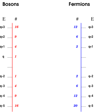
Figure 1: A schematic structure of the pairings among the modes. Here $E$ is the energy of the mode and $\#$ is the number of bosonic and fermionic modes with a given energy.

This structure of pairing and un-pairing among the modes is explicitly shown in the Figure 1. In general, for $j\geq 0$, we have the following structure

	$E_{+}$	Degeneration	$E_{-}$	Degeneration
Boson	$j+q$	$(j+1)^{2}$	$-j-2+q$	$(j+1)^{2}$
Fermion	$j+q$	$j(j+1)$	$-j-2+q$	$(j+1)(j+2)$

The BPS modes are the modes unpaired in this table, and they are counted by the superconformal index as explained above.

We can repeat the above procedure for the vector multiplet. In the case of the gaugino we have

Wave function	$E$	$(J_{3},\tilde{J}_{3})$
$b_{n}$	$j$	$\left(\frac{j-1}{2},\frac{j}{2}\right)$
$d_{n}^{\dagger}$	$-j-1$	$\left(\frac{j}{2},\frac{j-1}{2}\right)$

with $j\geq 1$. For the vector field one can expand in terms of the spin-1 spherical harmonics and the modes are

Wave function	$E$	$(J_{3},\tilde{J}_{3})$
$a_{n}$	$j+1$	$\left(\frac{j-1}{2},\frac{j+1}{2}\right)$
$c_{n}^{\dagger}$	$-j-1$	$\left(\frac{j+1}{2},\frac{j-1}{2}\right)$

with $j\geq 1$. By summing over all these states the contribution of the vector multiplet to the superconformal index is

$$I_{V}=\sum_{j,j_{3}\widetilde{j_{3}}}(-1)^{F}e^{-\tau\Xi}t^{H}y^{2\tilde{j}_{3}}=\frac{2t^{2}-t(y+1/y)}{(1-ty)(1-t/y)}$$ (27)

In the rest of this section we apply our prescription to obtain the BPS states in a different way, in which it is not necessary to solve for the whole spectrum. We start by considering the metric as in (18) with $a=b=1$. The two angles $\alpha$ and $\beta$ can be associated to the Cartan subgroup of the $SU(2)^{2}$ isometry group of the metric.

We start by solving the equation (9) for the BPS fermion in the chiral multiplet . Once we write the fermion as $\psi=\zeta F$ and solve the equation $\Delta_{\psi}\left(\zeta F\right)=0$, we expand $F$ as $F=e^{Et+in\alpha+im\beta}g_{\psi}(\theta)$, where $E$ is the eigenvalue associated to the $S^{1}$ and $n$ and $m$ are integer numbers associated to the two $SU(2)$ in the $S^{3}$, parameterized by the periodic coordinates $\alpha$ and $\beta$ in the metric. We obtain

$$\left\{\begin{array}[]{ccc}g_{\psi}^{\prime}+i\,g_{\psi}(2+E+m+n-q+i\,m\cot\theta-i\,n\tan\theta)&=&0\\ g_{\psi}^{\prime}-ig_{\psi}(2+E+m+n-q-i\,m\cot\theta+i\,n\tan\theta)&=&0\\ \end{array}\right.$$ (30)

These two equation can be simultaneously solved for $E=q-2-m-n$ and the solution is

$$g_{\psi}(\theta)=\sin^{m}\theta\cos^{n}\theta\qquad\qquad\mbox{for}\qquad\theta\sim 0,\pi/2$$ (31)

that is square integrable if $m,n\geq 0$ . This represents the contributions of the BPS fermion to the index. Because $E$ is negative, we have found that the corresponding state is an antiparticle mode of the fermion. Thus, when we plug its quantum numbers in the index, we have to flip their signs: the energy of the field is $E^{(\psi)}=-E=2-q+m+n$. The other operator that commutes with the supercharge is $\tilde{J}_{3}$ that has eigenvalues $m-n$. The fermionic contribution to the index is then

$$I_{\psi}=-\sum_{m,n\geq 0}t^{n+m+2-q}y^{m-n}=-\frac{t^{2-q}}{(1-ty)(1-t/y)}$$ (32)

We parameterize the BPS boson as $\phi=e^{Et+in\alpha+im\beta}g_{\phi}(\theta)$ and the equation (5) becomes

$$\left\{\begin{array}[]{ccc}g_{\phi}^{\prime}+ig_{\phi}(E+m+n-q-i\,m\cot\theta+i\,n\tan\theta)&=&0\\ g_{\phi}^{\prime}-ig_{\phi}(E+m+n-q+i\,m\cot\theta+i\,n\tan\theta)&=&0\\ \end{array}\right.$$ (35)

The two equations are compatible if $E=q-m-n$ and the solution is

$$g_{\phi}(\theta)=\frac{1}{\sin^{m}\theta\cos^{n}\theta}\qquad\qquad\mbox{for}\qquad\theta\sim 0,\pi/2$$ (36)

and square integrability imposes $m,n\leq 0$. The BPS boson that contributes to the index is the particle in the expansion in terms of creation and annihilation operators, with energy $E^{(\phi)}=E$. The bosonic index is

$$I_{\phi}=\sum_{m,n\geq 0}t^{n+m+q}y^{m-n}=\frac{t^{q}}{(1-ty)(1-t/y)}$$ (37)

We now turn to the vector multiplet. In the case of the gaugino we read the pairing map from the transformation of $F_{\mu\nu}$. The BPS modes are the solution of the equation

$$\partial_{\mu}(\tilde{\zeta}\bar{\sigma}_{\nu}\lambda)-\partial_{\nu}(\tilde{\zeta}\bar{\sigma}_{\mu}\lambda)=0$$ (38)

This equation is solved by

$$\tilde{\zeta}\bar{\sigma}_{\mu}\lambda=\partial_{\mu}\Phi$$ (39)

Alternatively, one can require that the SUSY variation for $v_{\mu}$ gives a purely longitudinal field. We then impose the usual ansatz dictated by the $U(1)$ symmetries

$$\Phi=e^{Et+i\alpha n+i\beta m}h_{\Phi}(\theta)\quad,\quad\lambda=e^{Et+i\alpha\left(n+\frac{1}{2}\right)+i\beta\left(m+\frac{1}{2}\right)}\left(\begin{array}[]{c}\lambda_{1}(\theta)\\ \lambda_{2}(\theta)\end{array}\right)$$ (40)

and we plug it in (39). Moreover we impose that $\lambda$ satisfies its equations of motion. In this way we find

$$E = -m-n$$

$$\lambda_{1}(\theta) = \frac{1}{\sqrt{2}}e^{\frac{i\theta}{2}}h_{\Phi}(\theta)\left(\frac{m}{\sin\theta}+i\frac{n}{\cos\theta}\right)$$

$$\lambda_{2}(\theta) = -\frac{1}{\sqrt{2}}e^{-\frac{i\theta}{2}}h_{\Phi}(\theta)\left(i\frac{m}{\sin\theta}+\frac{n}{\cos\theta}\right)$$

$$h_{\Phi}^{\prime}(\theta) = h_{\Phi}(\theta)\left(n\tan\theta-m\cot\theta\right)$$ (41)

The equation for $h_{\Phi}(\theta)$ tells us that the solution is square integrable for $m,n\leq 0$, but we exclude the vanishing solution corresponding to $(m,n)=(0,0)$. Thus the energy is positive and the gaugino contribution to the index is

$$I_{\lambda}=-\left(\sum_{m,n=-\infty}^{0}t^{-m-n}y^{m-n}-1\right)=\frac{t^{2}-t(y+1/y)}{(1-ty)(1-t/y)}$$ (42)

where the second term comes from subtracting the $(m,n)=(0,0)$ contribution.

The gauge field works as follows. First we impose that the BPS equation is satisfied

$$\sigma^{\mu\nu}\zeta F_{\mu\nu}=0$$ (43)

We consider the Abelian case and define the components of the EM field as $\mathcal{E}_{i}=F_{ti}$ and $2\mathcal{B}_{i}=\epsilon_{ijk}F_{jk}$ where the latin letters label the $S^{3}$ coordinates. We parametrize these fields with the ansatz

$$\mathcal{E}_{i}(t,\theta,\alpha,\beta)=e^{Et+i\alpha n+i\beta m}\mathcal{E}_{i}(\theta)\quad,\quad\mathcal{B}_{i}(t,\theta,\alpha,\beta)=e^{Et+i\alpha n+i\beta m}\mathcal{B}_{i}(\theta)$$ (44)

From (43) we derive the following three equations

$$\begin{split}\csc\theta\sec\theta\mathcal{B}_{\theta}+\mathcal{E}_{\theta}&\equiv y(\theta)\\ \csc\theta\mathcal{B}_{\alpha}+\sec\theta\mathcal{E}_{\alpha}&=-i\sin\theta\,y(\theta)\\ \sec\theta\mathcal{B}_{\beta}+\csc\theta\mathcal{E}_{\beta}&=i\cos\theta\,y(\theta)\end{split}$$ (45)

where $y(\theta)$ is arbitrary. The other equations are the Maxwell equation (or equivalently the Bianchi identities and the equations of motion). The equations of motion $\mathcal{D}_{\mu}F^{\mu\nu}=0$ are

$$\begin{split}-i\left(m\sec^{2}\theta\mathcal{E}_{\alpha}+n\csc^{2}\theta\mathcal{E}_{\beta}\right)+E_{\theta}-2\cot 2\theta\mathcal{E}_{\theta}-\mathcal{E}_{\theta}^{\prime}&=0\\ in\csc^{2}\theta\mathcal{B}_{\alpha}-im\sec^{2}\theta\mathcal{B}_{\beta}+E\,\mathcal{E}_{\theta}&=0\\ -in\csc^{2}\theta f^{2}\mathcal{B}_{\theta}+\tan\theta\mathcal{B}_{\beta}+E\,\mathcal{E}_{\alpha}-\mathcal{B}_{\beta}+\mathcal{B}_{\beta}^{\prime}&=0\\ -im\sec^{2}\theta\mathcal{B}_{\theta}+\cot\theta\mathcal{B}_{\alpha}+E\,\mathcal{E}_{\beta}+\mathcal{B}_{\alpha}\mathcal{B}_{\alpha}^{\prime}&=0\end{split}$$ (46)

and the Bianchi identities $\partial_{[\mu}F_{\nu\rho]}=0$ are

$$\begin{split}im\mathcal{B}_{\alpha}+in\mathcal{B}_{\beta}+\mathcal{B}_{\theta}^{\prime}&=0\\ E\mathcal{B}_{\beta}+im\mathcal{E}_{\theta}-\mathcal{E}_{\alpha}^{\prime}&=0\\ E\mathcal{B}_{\alpha}+in\mathcal{E}_{\theta}-\mathcal{E}_{\beta}^{\prime}&=0\\ E\mathcal{B}_{\theta}+in\mathcal{E}_{\alpha}-im\mathcal{E}_{\beta}&=0\end{split}$$ (47)

We then have eleven equations for seven variables (the energy and the non zero components of the electromagnetic fields). Even if the system looks overdetermined these equations are linearly dependent. By expressing every function in terms of $y(\theta)$ and $E$ we obtain

$$\left(\partial_{\theta}-(m-1)\cot\theta+(n-1)\tan\theta\right)y(\theta)=0\quad,\quad E=-m-n$$ (48)

The solution is square integrable for $m,n\geq 1$. In this case the contribution comes from the antiparticle in the mode expansion and the index is

$$I_{B}^{(V)}=\sum_{m=1}^{\infty}\sum_{n=1}^{\infty}t^{m+n}y^{n-m}=\frac{t^{2}}{(1-ty)(1-t/y)}$$ (49)

If we consider a non abelian gauge group we must add an extra chemical potential for the gauge symmetry. Indeed since the index is a topological invariant the gauge coupling does not play any role and we only need to take care of the fact that the vector multiplet transforms in the adjoint representation. The gauge invariant combinations are given by the Plethystic exponential after integrating over the Haar measure Aharony:2003sx ; Benvenuti:2006qr .

3.4 Squashed spheres

The superconformal index on the squashed sphere is expected to coincide with the one computed in the round limit, up to a redefinition of the variables. Indeed this manifold preserves the topological properties of $S^{3}$ and this guarantees that the index does not change under squashing.

This can be shown with a simple argument based on the definition of the index. Indeed the index on the three sphere is defined as

$${\cal I}_{S^{3}\times S^{1}}(t,y) = \text{Tr}(-1)^{F}e^{-\beta\{Q,Q^{\dagger}\}}t^{H}y^{2\tilde{J}_{3}}=\sum_{BPS}\text{Tr}(-1)^{F}t^{R-2\tilde{J}_{3}}y^{2\tilde{J}_{3}}$$ (50)

$$= \sum_{BPS}\text{Tr}(-1)^{F}t^{R+J_{\alpha}+J_{\beta}}y^{J_{\alpha}-J_{\beta}}$$

where $J_{\alpha}\equiv i\partial_{\alpha}$ and $J_{\beta}\equiv i\partial_{\alpha}$ are the generators of the two $U(1)$’s in the Hopf fibration. By defining $p=ty$ and $q=t/y$ the index becomes (this change of coordinates has been first considered in Dolan:2008qi )

$${\cal I}_{S^{3}\times S^{1}}(p,q)=\sum_{BPS}\text{Tr}(-1)^{F}p^{R/2+J_{\alpha}}q^{R/2+J_{\beta}}$$ (51)

The same definition of the index on the squashed sphere is

$${\cal I}_{S^{3}\times S^{1}}(t,y) = \text{Tr}(-1)^{F}e^{-\beta\{Q,Q^{\dagger}\}}t^{H}y^{2\tilde{J}_{3}+\frac{R}{2}\left(\frac{1}{a}-\frac{1}{b}\right)}$$ (52)

$$= \sum_{BPS}\text{Tr}(-1)^{F}t^{\frac{R}{2}\left(\frac{1}{a}+\frac{1}{b}\right)+\frac{J_{\alpha}}{a}+\frac{J_{\beta}}{b}}y^{\frac{J_{\alpha}}{a}-\frac{J_{\beta}}{b}+\frac{R}{2}\left(\frac{1}{a}-\frac{1}{b}\right)}$$

By defining $p=(ty)^{\frac{1}{a}}$ and $q=(t/y)^{\frac{1}{b}}$ the index on the squashed sphere is defined as (51) and its definition coincides with the one for the round case as expected. Then the index is expected to coincide because the two spaces have the same topology, and the same BPS states contributing to the index in the round case contribute to the index in the squashed case.

In this section we explicitly show this result by exploiting the power of our prescription for the identification of the BPS states. Indeed there are no known result for expansion in terms of harmonics on these spaces and a direct calculation is not at hand.

We start by writing the fermion in the chiral multiplet as $\psi=\zeta F$ and solve the equation $\Delta_{\psi}\left(\zeta F\right)=0$, where we expand $F$ as $F=e^{Et+in\alpha+im\beta}g_{\psi}(\theta)$, obtaining the following set

$$\left\{\begin{array}[]{l}g_{\psi}^{\prime}=-\frac{e^{-i\theta}g_{\psi}}{2ab}\left(2abe^{i\theta}(iEf-(q-2)\cot{2\theta})+f\left(\frac{(a(q-2(m+1))}{\sin\theta}+\frac{ib(2(n+1)-q)}{\cos\theta}\right)\right)\\ g_{\psi}^{\prime}=\frac{g_{\psi}}{2ab}\left(\frac{2ab(q-2)}{\tan 2\theta}+f\left(\frac{ae^{i\theta}(2(m+1)-q)}{\sin\theta}+\frac{ib(2aE+(2(n+1)-q)(1+i\tan\theta))}{\cos\theta}\right)\right)\\ \end{array}\right.$$

These two equations can be simultaneously solved if

$$E=\frac{q}{2}\left(\frac{1}{a}+\frac{1}{b}\right)-\frac{1}{a}-\frac{1}{b}-\frac{n}{a}-\frac{m}{b}$$ (54)

Square integrability requires the quantum numbers $m,n\geq 0$ as in the case of the sphere. The mode contributing to the index is an antiparticle and its energy is $E_{\psi}=-E$. By summing over the BPS states we have

$$I_{\psi}=-\frac{(t/y)^{\frac{2-q}{2b}}(ty)^{\frac{2-q}{2a}}}{\left(1-(t/y)^{\frac{1}{b}}\right)\left(1-(ty)^{\frac{1}{a}}\right)}$$ (55)

The equations for the scalar $\phi=e^{Et+i\alpha m+i\beta m}g_{\phi}(\theta)$ become

$$\left\{\begin{array}[]{l}g_{\phi}^{\prime}=-\frac{g_{\phi}}{2ab}\left(\frac{2abq}{\tan 2\theta}+f\left(2iabE+e^{i\theta}\left(\frac{a(2m-q)}{\sin\theta}+\frac{ib(2n-q)}{\cos\theta}\right)\right)\right)\\ g_{\phi}^{\prime}=-\frac{g_{\phi}e^{-i\theta}}{2ab}\left(\frac{2abqe^{i\theta}}{\tan 2\theta}+f\left(\frac{a(2m-q)}{\sin\theta}-ib\left(2ae^{i\theta}E+\frac{(2n-q)}{\cos\theta}\right)\right)\right)\end{array}\right.$$ (58)

They can be simultaneously solved if

$$E=\frac{q}{2}\left(\frac{1}{a}+\frac{1}{b}\right)-\frac{n}{a}-\frac{m}{b}$$ (59)

with $m,n\leq 0$. This constraint fixes $E_{\phi}=E$ and the index for the scalar field in the chiral multiplet is

$$I_{\phi}=\frac{(t/y)^{\frac{q}{2b}}(ty)^{\frac{q}{2a}}}{\left(1-(t/y)^{\frac{1}{b}}\right)\left(1-(ty)^{\frac{1}{a}}\right)}$$ (60)

Note that the two single particle indices that we have found only depend on the two parameters $(ty)^{1/a}$ and $(t/y)^{1/b}$. Thus, the following redefinition of the fugacities

$$t\to t^{\frac{a+b}{2}}y^{\frac{a-b}{2}}\quad,\quad y\to t^{\frac{a-b}{2}}y^{\frac{a+b}{2}}$$ (61)

gives ${\cal I}_{\rm sphere}={\cal I}_{\rm squash}$. The transformation (61) does not modify the physical content of the index, because the fugacities are, a priori, arbitrary parameters. The only constraints come from the requirement of convergence of the index, and are given by $ty<1$ and $t/y>1$ Kinney:2005ej . Of course, the latter are preserved by equation (61) for positive $a$ and $b$.

On the squashed sphere, the gaugino equation (3.3) gives

$$\lambda_{1}(\theta) = \frac{e^{\frac{i\theta}{2}}}{\sqrt{2}}h(\theta)\left(\frac{m}{b\sin\theta}+i\frac{n}{a\cos\theta}\right)\,,\quad\lambda_{2}(\theta)=-\frac{e^{-\frac{i\theta}{2}}}{\sqrt{2}}h(\theta)\left(i\frac{m}{b\sin\theta}+\frac{n}{a\cos\theta}\right)$$

$$E = -\frac{n}{a}-\frac{m}{b}\quad\quad\quad\quad\quad\quad\quad\quad\,\,\,,\quad\quad h^{\prime}(\theta)=f(\theta)h(\theta)\left(\frac{n}{a}\tan\theta-\frac{m}{b}\cot\theta\right)$$

The solution for $\lambda$ is square integrable if $m,n\leq 0$, but we exclude the mode $(m,n)=(0,0)$ because it is identically vanishing. The sum over the gaugino states gives

$$I_{\lambda}=-\left(\sum_{m=0}^{-\infty}\sum_{n=0}^{-\infty}t^{-\frac{n}{a}-\frac{m}{b}}y^{\frac{n}{a}-\frac{m}{b}}-1\right)=-\frac{(t/y)^{\frac{1}{b}}(ty)^{\frac{1}{a}}-(t/y)^{\frac{1}{b}}-(ty)^{\frac{1}{a}}}{\left(1-(t/y)^{\frac{1}{b}}\right)\left(1-(ty)^{\frac{1}{a}}\right)}$$ (62)

For the gauge bosons the equations (43) become

$$\begin{split}\frac{\csc\theta\sec\theta\mathcal{B}_{\theta}}{ab}+\frac{\mathcal{E}_{\theta}}{f}&\equiv y(\theta)\\ \frac{\csc\theta\mathcal{B}_{\alpha}}{bf}+\frac{\sec\theta\mathcal{E}_{\alpha}}{a}&=-i\sin\theta\,y(\theta)\\ \frac{\sec\theta\mathcal{B}_{\beta}}{af}+\frac{\csc\theta\mathcal{E}_{\beta}}{b}&=i\cos\theta\,y(\theta)\end{split}$$ (63)

After applying the equations of motions

$$\begin{split}-if^{2}\left(\frac{m\sec^{2}\theta\mathcal{E}_{\alpha}}{a^{2}}+\frac{n\csc^{2}\theta\mathcal{E}_{\beta}}{b^{2}}\right)+\frac{\mathcal{E}_{\theta}f^{\prime}}{f}-2\cot 2\theta\mathcal{E}_{\theta}-\mathcal{E}_{\theta}^{\prime}&=0\\ \frac{in\csc^{2}\theta\mathcal{B}_{\alpha}}{b^{2}}-\frac{im\sec^{2}\theta\mathcal{B}_{\beta}}{a^{2}}+E\mathcal{E}_{\theta}&=0\\ -\frac{in\csc^{2}\theta f^{2}\mathcal{B}_{\theta}}{b^{2}}+\tan\theta\mathcal{B}_{\beta}+Ef^{2}\mathcal{E}_{\alpha}-\frac{\mathcal{B}_{\beta}f^{\prime}}{f}+\mathcal{B}_{\beta}^{\prime}&=0\\ -\frac{imf^{2}\sec^{2}\theta\mathcal{B}_{\theta}}{a^{2}}+\cot\theta\mathcal{B}_{\alpha}+Ef^{2}\mathcal{E}_{\beta}+\frac{\mathcal{B}_{\alpha}f^{\prime}}{f}-\mathcal{B}_{\alpha}^{\prime}&=0\end{split}$$ (64)

and the Bianchi identities

$$\begin{split}im\mathcal{B}_{\alpha}+in\mathcal{B}_{\beta}+\mathcal{B}_{\theta}^{\prime}&=0\\ E\mathcal{B}_{\beta}+im\mathcal{E}_{\theta}-\mathcal{E}_{\alpha}^{\prime}&=0\\ E\mathcal{B}_{\alpha}+in\mathcal{E}_{\theta}-\mathcal{E}_{\beta}^{\prime}&=0\\ E\mathcal{B}_{\theta}+in\mathcal{E}_{\alpha}-im\mathcal{E}_{\beta}&=0\end{split}$$ (65)

we find

$$\left(\frac{\partial_{\theta}}{f(\theta)}-\left(\frac{m}{b}-\frac{1}{f(\theta}\right)\cot\theta+\left(\frac{n}{a}-\frac{1}{f(\theta)}\right)\tan\theta\right)y(\theta)=0\quad,\quad E=-\frac{n}{a}-\frac{m}{b}$$ (66)

and the index is

$$I_{B}^{(V)}=\sum_{m=1}^{\infty}\sum_{n=1}^{\infty}t^{\frac{n}{a}+\frac{m}{b}}y^{\frac{n}{a}-\frac{m}{b}}=\frac{(t/y)^{\frac{1}{b}}(ty)^{\frac{1}{a}}}{\left(1-(t/y)^{\frac{1}{b}}\right)\left(1-(ty)^{\frac{1}{a}}\right)}$$ (67)

4 Example: reducing $4d$ indices to $3d$ partition functions

In this section we revisit the reduction of the four dimensional superconformal index to the three dimensional partition function Kapustin:2009kz ; Jafferis:2010un ; Hama:2010av . We will show that the reduction follows very easily, and the same argument can be generalized to other dimensions. The example of the round sphere can be found in Dolan:2011rp ; Gadde:2011ia ; Imamura:2011uw .

For concreteness, we consider the index on $S_{b}^{3}\times S^{1}$ and show that it reduces to the three-dimensional partition function ${\cal Z}_{S^{3}_{b}}$ by dimensional reduction. In four dimensions we consider the multi-particle index for a chiral and a vector multiplet, that takes into account all the multi-trace gauge invariant combinations. The multi-particle index can be found by taking the Plethystic exponential of the single particle index (1)

$${\cal I}_{m.p.}=\text{Exp}\left[\sum_{k=1}^{\infty}\frac{{\cal I}_{s.p.}(t^{k},y^{k},f^{k},g^{k})}{k}\right]$$ (68)

Comparing to equation (1), we have added two more parameters to the single particle index: the fugacity $f$ for the internal flavor symmetries and the one $g$ for the gauge symmetry. In the rest of this section we consider only the $f,y\to 1$ limit.

We start by looking at the contribution of the chiral multiplet. As we already pointed out the fields contributing to the index on $S_{b}^{3}\times S^{1}$ are the particle $\phi$ for the bosonic component and the antiparticle $\psi^{\dagger}$ for the fermionic component. If one component is in the $\rho$ representation of the gauge group, than the other component is in the $\bar{\rho}$. By recalling the single particle result

$${\cal I}_{\Phi}={\cal I}_{\phi}+{\cal I}_{\psi}=\sum_{BPS}\left(t^{E_{\phi}}g^{\rho}-t^{E_{\psi}}g^{-\rho}\right)$$ (69)

the multi-trace contribution to the superconformal index from a chiral multiplet in the $\rho$ representation of the gauge group is

$$\text{Exp}\left[\sum_{k=1}^{\infty}\frac{1}{k}\sum_{BPS}\left(t^{kE_{\phi}+ik\sigma\rho}-t^{kE_{\psi}-ik\sigma\rho}\right)\right]$$ (70)

that becomes

$$\prod_{BPS}\frac{1-t^{E_{\phi}+i\sigma\rho}}{1-t^{E_{\psi}-i\sigma\rho}}\,\,\stackrel{{\scriptstyle t\to 1}}{{\longrightarrow}}\,\,\prod_{BPS}\frac{E_{\phi}+i\sigma\rho}{E_{\psi}-i\sigma\rho}$$ (71)

where we identified the chemical potential for the gauge group $g$ with $t^{i\sigma}$, where $\sigma$ is the solution to the three-dimensional saddle point equations (or to the four-dimensional zero energy supersymmetry equations), which set $\sigma$ to a constant Kapustin:2009kz .

The product in (71) ranges over the set of BPS states. As we have seen, this set is labeled by the Cartan subgroup of the three-dimensional isometry group, which in the case at hand consists of the two $U(1)$ symmetries $U(1)_{\alpha}$ and $U(1)_{\beta}$ that rotate the Hopf angles independently. If we identify the fugacity $t$ with $e^{-\tau}$, where $\tau$ is the period of the time direction, then the limit in (71) corresponds to shrinking the time circle to zero size, i.e. to dimensional reduction. Indeed the right hand side of (71) is the one loop exact contribution of the chiral multiplet to the three-dimensional partition function found in Hama:2011ea . The energies $E_{\phi}$ and $E_{\psi}$ of the BPS states in four dimensions, obtained with the procedure explained in section 2, become the eigenvalues of the unpaired states in the three dimensional case. An analogous derivation can be performed for the vector multiplet.

We expect that our correspondence and the reduction are more general than shown here and that they apply generically to $\mathcal{M}_{d-1}\times S^{1}\rightarrow\mathcal{M}_{d-1}$ , provided at least two real supersymmetries are preserved. The result (71) should apply to any $(d-1)$-dimensional theory, if its field content may be derived by dimensional reduction of a corresponding $d$-dimensional model. The $(d-1)$-dimensional saddle points and the quantum corrections may be derived by the $d$-dimensional analysis, but in the full partition function there may be an additional contribution, denoted $S_{\ast}$ in (2), due to a classical term which does not have an uplift to $d$-dimensions. This is the case, for instance, for the Chern-Simons term in the three dimensional case. However, once the $(d-1)$-dimensional action is known, one can plug the saddle point configuration in it and obtain also the classical term.

It is interesting to compare with the known results in the literature. To the best of our knowledge, this is the first time that the superconformal index on a squashed sphere is computed explicitly. Of course, because it is identical to the one on the round sphere up to a redefinition of the fugacities, one can consider reducing the latter to the partition function on the squashed sphere. This is usually done by taking an ad hoc limit instead of the one in (71) Dolan:2011rp . Namely, we can reinterpret those results by stating that one can squash the chemical potentials without affecting the physical meaning of the index, and then take the natural limit $t\to 1$ to shrink the time circle. The necessary redefinitions are not known in general, and we believe that our results offer a very clean physical interpretation and can be easily generalized.

5 The conjecture in other dimensions and manifolds

From the discussion in section 4 we see that our results can be more general than stated until now. We propose that the same one-to-one map described there holds in more general cases, like in other dimensions, manifolds and for extended supersymmetric theories.

Localization on a three-sphere does not give rise to any non-perturbative (instanton or monopole) contribution, and this is in full agreement with the BPS correspondence we have proposed. However the localizing term in different dimensions can lead to a sum over the instantons as happens, for instance, on the four-sphere. If our argument can be applied also in that case, the five-dimensional BPS equations should contain all the quantum information also about the non-perturbative states.

In section 2 we have mostly focused on a three-dimensional manifold whose Cartan subgroup is $U(1)^{2}$, and thus there are two well-defined quantum numbers, one can break the Cartan to $U(1)$ and still preserve two real supersymmetries. In this case one has only one integer quantum number to sum over, and the BPS conditions will give constraints on its range.

6 General partition functions via an uplift to an index

We have observed above that the reduction of the superconformal index on $\mathcal{M}_{d-1}\times S^{1}$ to the partition function on $\mathcal{M}_{d-1}$ highlights the relation between the BPS states in $d$ dimensions and the $d-1$ dimensional unpaired states. Equivalently one can obtain the three dimensional partition function on $\mathcal{M}_{d-1}$ by uplifting the supersymmetry from $\mathcal{M}_{d-1}$ to $\mathcal{M}_{d-1}\times S^{1}$. The $d$-dimensional Killing spinors are independent from the $S^{1}$ and the $d$ dimensional unpaired states are preserved by shrinking the circle. Even if this procedure is similar to the reduction explained in section 2 it is interesting to investigate the problem in this way because it shows the relation of our construction and localization. Indeed the $d-1$-dimensional saddle point equations coincide with the zero energy equations of the $d$-dimensional problem. We now exploit this fact to simplify the computation of the exact partition function itself.

Consider a $d$-dimensional field theory ${\cal F}_{d}$ and its dimensional reduction to ${\cal F}_{d-1}$, which preserves the same amount of supersymmetry. We can place ${\cal F}_{d-1}$ on a curved manifold ${\cal M}_{d-1}$ and localize the corresponding path integral to an at most finite dimensional integral by picking two real conserved supercharges and solving the corresponding equation $|\delta\psi_{d-1}|^{2}=0$, where $\psi$ is any fermion of the theory. This is the same as picking the uplifted supercharges on ${\cal M}_{d}$ and solving for

$$|\delta\Psi_{d}|^{2}\Big{|}_{E=0}=0$$ (72)

where $\Psi_{d}\sim\Psi_{d-1}e^{Et}$ is the set of fermions in the ${\cal F}_{d}$ theory, and gives the loci that solve the saddle point equations in the path integral. Denote the latter by $\Phi_{\ast}$ and the classical action $S(\Phi_{\ast})\equiv S_{\ast}$. The exact path integral on ${\cal M}_{d-1}$ is now given by

$$Z_{{\cal M}_{d-1}}\sim\int\left[d\Phi\right]\,\,e^{-S_{\ast}}\frac{{\rm Pf}D_{F}}{\sqrt{\det{D_{B}}}}$$ (73)

where $[d\Phi]$ is the measure over the loci $\Phi_{\ast}$, and in general $D_{F}$ and $D_{B}$ are respectively a first order and second order differential operator derived by a $(d-1)$-dimensional Q-exact action. Notice that we did not compute any Q-exact action, so we do not know the explicit form of $D_{F}$ and $D_{B}$, but we know that $\Phi_{\ast}$ are their zero modes. In general, we should find the spectrum of their eigenvalues around the solutions of (72), and it turns out that many of them simplify between the numerator and the denominator in (73) due to supersymmetry. The ones that do not simplify are obtained with the procedure explained in section 2.

To summarize we can derive the spectrum of eigenvalues necessary to compute the exact partition function in $d-1$ dimensions (73) by finding the energy eigenvalues from a corresponding set of first order differential operators in $d$ dimensions. We do not need the Lagrangian giving the equations of motion for ${\cal F}_{d}$, but only the supersymmetry transformations of the matter multiplets that appear there. This means that we only need the uplift of the conserved supercharges, without worrying about the uplift of the Lagrangian.

Appendix A More on the gauge field contribution

In this Appendix we show a different approach to compute the contribution of the gauge field to the index. We focus on the four-dimensional case of $S^{1}\times S^{3}_{b}$, and the round sphere can be obtained by taking the $a,b\to 1$ limit.

As explained in the main text, our method relies on finding a map from the bosonic modes to the fermionic ones such that their contributions to the index cancel out, and the unpaired modes are identified with the BPS states. We have seen that the normal modes of the gauge field strength can be mapped to the gaugino modes. Among the unpaired modes of the gauge field strength, those which also satisfy the Maxwell equations are the BPS modes. Here we offer another interpretation for the latter.

Besides the map between the gauge and the gaugino, we can find another map that relates a mode of the gauge field strength to a fermion with the same $(\Xi,H,\tilde{J}_{3})$ quantum numbers

$$\delta\chi=\tilde{\zeta}\tilde{\sigma}^{\mu}v_{\mu}$$ (74)

The field $\chi$ is a pure supergauge field, i.e. it is set to zero in the Wess-Zumino gauge. For this reason it does not belong to the Hilbert space and every gauge field such that

$$\tilde{\zeta}\tilde{\sigma}^{\mu}v_{\mu}=0$$ (75)

can contribute to the index. The solution to this equation is

$$\begin{split}v_{1}&=0\\ v_{2}&=Y(\theta)e^{Et+i(n\alpha+m\beta)}\\ v_{3}&=ia\frac{\sin{\theta}\cos{\theta}}{f(\theta)}Y(\theta)e^{Et+i(n\alpha+m\beta)}\\ v_{4}&=-ib\frac{\sin{\theta}\cos{\theta}}{f(\theta)}Y(\theta)e^{Et+i(n\alpha+m\beta)}\end{split}$$ (76)

where the first line is a gauge choice and $Y(\theta)$ is to be determined. Then the two equations $\sigma^{\mu\nu}F_{\mu\nu}\zeta=0$ for $Y(\theta)$ give

$$E=-\frac{n}{a}-\frac{m}{b}$$ (77)

for $n,m\leq 1$. This is the same result that we obtained in section 3. Notice that equation (75) is satisfied by the pure gauge configuration $v_{\mu}=\partial_{\mu}\Phi$ that appears in equation (39).

References

- (1) E. Witten, Constraints on Supersymmetry Breaking, Nucl.Phys. B202 (1982) 253.
- (2) S. Cecotti and L. Girardello, Functional Measure, Topology and Dynamical Supersymmetry Breaking, Phys.Lett. B110 (1982) 39.
- (3) C. Romelsberger, Counting chiral primaries in N = 1, d=4 superconformal field theories, Nucl.Phys. B747 (2006) 329–353, [hep-th/0510060].
- (4) J. Kinney, J. M. Maldacena, S. Minwalla, and S. Raju, An Index for 4 dimensional super conformal theories, Commun.Math.Phys. 275 (2007) 209–254, [hep-th/0510251].
- (5) E. Witten, Quantum Field Theory and the Jones Polynomial, Commun.Math.Phys. 121 (1989) 351.
- (6) V. Pestun, Localization of gauge theory on a four-sphere and supersymmetric Wilson loops, Commun.Math.Phys. 313 (2012) 71–129, [arXiv:0712.2824].
- (7) D. Sen, FERMIONS IN THE SPACE-TIME R x S**3, J.Math.Phys. 27 (1986) 472.
- (8) D. Sen, SUPERSYMMETRY IN THE SPACE-TIME R x S**3, Nucl.Phys. B284 (1987) 201.
- (9) S. Nawata, Localization of N=4 Superconformal Field Theory on and Index, JHEP 1111 (2011) 144, [arXiv:1104.4470].
- (10) F. Dolan, V. Spiridonov, and G. Vartanov, From 4d superconformal indices to 3d partition functions, Phys.Lett. B704 (2011) 234–241, [arXiv:1104.1787].
- (11) A. Gadde and W. Yan, Reducing the 4d Index to the Partition Function, arXiv:1104.2592.
- (12) Y. Imamura, Relation between the 4d superconformal index and the partition function, JHEP 1109 (2011) 133, [arXiv:1104.4482].
- (13) N. Hama, K. Hosomichi, and S. Lee, SUSY Gauge Theories on Squashed Three-Spheres, JHEP 1105 (2011) 014, [arXiv:1102.4716].
- (14) G. Festuccia and N. Seiberg, Rigid Supersymmetric Theories in Curved Superspace, JHEP 1106 (2011) 114, [arXiv:1105.0689].
- (15) M. F. Sohnius and P. C. West, An Alternative Minimal Off-Shell Version of N=1 Supergravity, Phys.Lett. B105 (1981) 353.
- (16) M. Sohnius and P. C. West, THE TENSOR CALCULUS AND MATTER COUPLING OF THE ALTERNATIVE MINIMAL AUXILIARY FIELD FORMULATION OF N=1 SUPERGRAVITY, Nucl.Phys. B198 (1982) 493.
- (17) T. T. Dumitrescu, G. Festuccia, and N. Seiberg, Exploring Curved Superspace, JHEP 1208 (2012) 141, [arXiv:1205.1115].
- (18) C. Klare, A. Tomasiello, and A. Zaffaroni, Supersymmetry on Curved Spaces and Holography, JHEP 1208 (2012) 061, [arXiv:1205.1062].
- (19) O. Aharony, J. Marsano, S. Minwalla, K. Papadodimas, and M. Van Raamsdonk, The Hagedorn - deconfinement phase transition in weakly coupled large N gauge theories, Adv.Theor.Math.Phys. 8 (2004) 603–696, [hep-th/0310285].
- (20) S. Benvenuti, B. Feng, A. Hanany, and Y.-H. He, Counting BPS Operators in Gauge Theories: Quivers, Syzygies and Plethystics, JHEP 0711 (2007) 050, [hep-th/0608050].
- (21) F. Dolan and H. Osborn, Applications of the Superconformal Index for Protected Operators and q-Hypergeometric Identities to N=1 Dual Theories, Nucl.Phys. B818 (2009) 137–178, [arXiv:0801.4947].
- (22) A. Kapustin, B. Willett, and I. Yaakov, Exact Results for Wilson Loops in Superconformal Chern-Simons Theories with Matter, JHEP 1003 (2010) 089, [arXiv:0909.4559].
- (23) D. L. Jafferis, The Exact Superconformal R-Symmetry Extremizes Z, arXiv:1012.3210.
- (24) N. Hama, K. Hosomichi, and S. Lee, Notes on SUSY Gauge Theories on Three-Sphere, JHEP 1103 (2011) 127, [arXiv:1012.3512].