Exact results for fixation probability of bithermal evolutionary graphs.

Abstract

One of the most fundamental concepts of evolutionary dynamics is the “fixation” probability, i.e. the probability that a mutant spreads through the whole population. Most natural communities are geographically structured into habitats exchanging individuals among each other and can be modeled by an evolutionary graph (EG), where directed links weight the probability for the offspring of one individual to replace another individual in the community. Very few exact analytical results are known for EGs. We show here how by using the techniques of the fixed point of Probability Generating Function, we can uncover a large class of of graphs, which we term bithermal, for which the exact fixation probability can be simply computed.

1 Introduction.

Evolutionary dynamics is a stochastic process due to competition between deterministic selection pressure and stochastic events due to random sampling from one generation to the other. One of the most fundamental concepts of evolutionary dynamics is the fixation probability, i.e. the probability that a mutant spreads and takes over the whole community(Patwa and Wahl [12]). In the framework of the Moran model (Moran [11]) for a well mixed population, where an individual’s offspring can replace any other one in the community, the fixation probability is

$$\pi_{f}=\frac{1-r^{-m_{0}}}{1-r^{-M}}$$ (1)

where $M$ is the size of the community, $m_{0}$ the original number of mutants and $r$ the relative fitness of the mutants. A similar result was reached by Kimura (Kimura [7]) for the Fisher-Wright model under the diffusion approximation.

The idea of well mixed population is however far from realistic. Natural communities are geographically extended and subdivided into patches that exchange individuals (figure 1a). Maruyama (Maruyama [9, 10]) was the first to cast the problem of evolutionary dynamics into a Moran process on graphs (or islands, in his terminology) and under harsh approximations, concluded that the fixation probability does not depend on the population structure. The first formal proof that Maruyama’s results are not always correct was given by Lieberman et al(Lieberman et al. [8]) who showed that for a Moran process on a star graph (Figure 1b), the effective fitness of the mutant, in the large population limit, can be enhanced to $r^{2}$ due to topological effects. In order to do so, Lieberman et al. considered evolutionary graphs (EG) where nodes contain exactly one individual, whether wild type or mutant, connected by directed links representing the geographical (or social) connectivity.

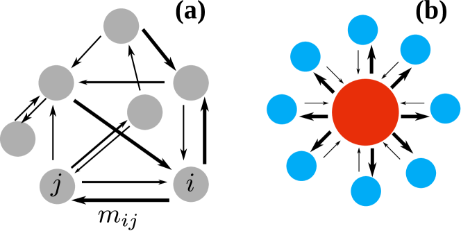
Figure 1: Evolutionary Graphs. (a) individuals are spread in space. A node $i$ can send its offspring only to connected nodes $j$ with a probability $m_{ij}$. A non-structure population can be considered as a fully connected graph with uniform migration probability $m_{ij}=1/N$. (b) The star configuration, which can be proved to differ from a non-structured population for its fixation probability.

Lieberman et al. also extended their results to the funnel topology with $K$ layers where the effective fitness, in the limit of large population, can be amplified to $r^{K}$, but provided only a sketch of the proof. Beyond the special cases considered by Lieberman et al, very few exact analytical results are known. A review of the present state of known results is given by Shakarian et al(Shakarian et al. [13]).

Most of the results of the EG are obtained through Monte Carlo numerical simulations. These simulations however scale as $2^{M}$ where $M$ is the number of nodes. A new numerical scheme has been proposed (Barbosa et al. [2]) to accelerate the speed of these simulations, but the computation of the fixation probability of large graphs is still very time consuming.

It would therefore be important to know the exact fixation probability of a large class of graphs that can be used as an approximation of closely related graphs or as a benchmark for assessing the progress in numerical simulation schemes. This is the aim of the present article.

We recently proposed a new method (Houchmandzadeh and Vallade [6]), based on the fixed points of the time dependent Probability Generating Function (fp-PGF) which can efficiently approximate the fixation probability of large, arbitrary graphs by solving only a system of $M$ second order algebraic equations. We show in the present article that the fp-PGF method can also be used to derive exact results for a large class of graphs that we call bithermal, which are an extension of the isothermal graphs considered by Lieberman et al.

The temperature of a node is related to the imbalance between the sum of the weights of the incoming and outgoing links. In isothermal graphs, all nodes are balanced and have the same temperature $T=1$. Bithermal graphs are bipartite, with two kinds of nodes at either temperature $T_{A}$ or $T_{B}$. The star topology (figure 1b) is one particular example of such graphs, some other particular examples are shown in Figure 2

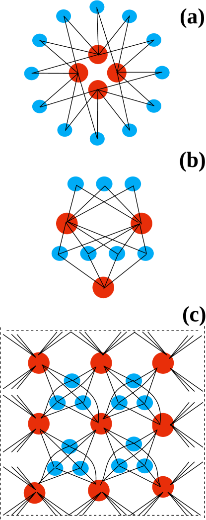
Figure 2: Some examples of bithermal graphs; for simplicity, each link represents two directed links. A bithermal graph is constituted of two kinds of nodes at respective temperature $T_{A}$ and $T_{B}$, indicated here by their colors. Each $A$ node is connected to a subset of $B$ nodes and vice versa. (a) a (4,12,6,2) generalized star, consisting of 4 central nodes and 12 peripheral nodes, each central node connected to 6 peripheral and each peripheral connected to two central nodes ; (b) an example where the combined effect of the number of links and their weight makes the graph bithermal ; (c) A symmetric 2 dimensional, bithermal crystal with periodic boundaries;

. We show here that the fixation probability of these graphs is a simple rational function of the fitness $r$ and of the number of nodes $M_{A}$ and $M_{B}$ in each class

$$\pi_{f}=f(M_{A},M_{B},r)$$

The exact expression of this function is given by equation (21) and its plot by figure 4a. When there is the same number of nodes in each class ($M_{A}=M_{B}$), bithermal graphs become isothermal and the function $f$ above is equal to the Moran expression (1). When the imbalance between the number of nodes in each class is large ($M_{A}\gg M_{B}$ or $M_{A}\ll M_{B}$), the fixation probability tends toward $0$ or $1-1/r^{2}$, depending on the nature of the Moran process (birth-death or death-birth).

This article is organized as follow. In the next section, we recall the continuous time stochastic process of Moran on graph and its associated Master equation ; the third section is devoted to the Probability Generating Function method ; In the fourth section, we apply these results to the bithermal graphs and give their exact fixation probability. The last section is devoted to some generalizations and conclusions.

2 Continuous time Moran process on graph.

Consider a community of $M$ individuals, which can either be wild type (WT) with fitness $1$ or mutant with relative fitness $r=1+s$. The individuals are spread spatially and the progeny of an individual $i$ can replace individual $j$ according to a connectivity map. The connectivity map can be envisioned as a graph, where each node $i$ contains exactly one individual, either mutant or wild type ; the weight of a link $m_{ij}$ specifies the probability for the progeny of an individual at node $i$ to replace an individual at node $j$ (Figure 1a). The coefficients $m_{ij}$ are collected into a connectivity matrix $\mathbf{m}$. As the number of individual is fixed, it is sufficient to specify the number of mutants (0 or 1) on each node $\mathbf{n}=(n_{1},n_{2},...n_{M})$ at a given time to have complete information about the system at this time. We consider here a continuous time model where birth (or death) events occur randomly with rate $\mu$ (Houchmandzadeh and Vallade [5]). The probability density for a node $i$ to decrease or increase its number of mutants by one unit during a time interval $dt$ is (Houchmandzadeh and Vallade [6])

$$W_{i}^{-}(n_{i}) = (\mu/M)n_{i}\sum_{k=1}^{M}m_{ki}(1-n_{k})$$ (2)

$$W_{i}^{+}(n_{i}) = (\mu/M)r\left(1-n_{i}\right)\sum_{k=1}^{M}m_{ki}n_{k}$$ (3)

It is crucial at this step to distinguish between two kinds of Moran processes (Antal et al. [1]). In the first case which we call D-B (Death first and then replacement, also called Voter Model), a death occurs first on a node, then immediately one connected node duplicates and send its progeny to this node. Equation (2) is therefore the probability density that a mutant dies at node $i$ during $dt$, and is replaced by the progeny of a WT on a connected node $k$. Equation (3) is the probability density that a WT dies at node $i$ and is replaced by a mutant on a connected node. Without loss of generality, the mutant’s advantage $r$ is included in this line, either as a decreased mortality or a better replacement success once a death event has occurred.

In the case of B-D processes (also called Invasion Process), a birth occurs first on a node $k$ and the progeny is then sent to a connected node $i$ to replace the local resident. The transition probabilities are still expressed by the same equations (2,3), but the quantity $\mu$ now denotes the birth rate.

Although the rate equations (2,3) are similar for these two processes, the normalization conditions of $m_{ki}$ coefficients are different :

$$\sum_{i=1}^{M}m_{ik}=1\,\,(\mbox{D-B});\,\,\sum_{i=1}^{M}m_{ki}=1\,\,(\mbox{B-D})\,\,\forall k$$ (4)

The temperature of a node is defined for these processes as

$$\sum_{i=1}^{M}m_{ki}=T_{k}\,\,\mbox{(D-B)\,\,;\,\,}\sum_{i=1}^{M}m_{ik}=T_{k}\,\,(\mbox{B-D})\,\,\forall k$$ (5)

Because of the normalization constraint (4), we must have $\sum_{j=1}^{M}T_{j}=M$ for both processes. This means that if some nodes are cold ($T<1$), others must be hot ($T>1$).

The Moran process is a one-step stochastic one, where during an infinitesimal interval $dt$, only one birth or death event can occur. Equations (2,3) are transition probabilities between states $\mathbf{n}$ on the one hand and states $a_{i}\mathbf{n}=(n_{1},...n_{i}-1,...n_{M})$ and $a_{i}^{\dagger}\mathbf{n}=(n_{1},...n_{i}+1,...n_{M})$ on the other. The probability $P(\mathbf{n},t)$ of observing state $\mathbf{n}$ at time $t$ obeys the Master equation

$$\frac{\partial P(\mathbf{n},t)}{\partial t}=\sum_{\{\mathbf{m}\}}W(\mathbf{m}\rightarrow\mathbf{n})P(\mathbf{m},t)-W(\mathbf{n}\rightarrow\mathbf{m})P(\mathbf{n},t)$$ (6)

The EG process we are considering has two absorbing states $\mathbf{1}=(1,1,...1)$ and $\mathbf{0}=(0,0,...0)$. Once a mutant has invaded all the nodes or has been eliminated from all of them, it is fixed or lost and there is no further evolution (until a new mutant appears by random mutation) : $W(\mathbf{1}\rightarrow\mathbf{m})=0$ and $W(\mathbf{0}\rightarrow\mathbf{m})=0$ as can be deduced from equations (2,3). Note that the probability of reaching state $\mathbf{1}$ from an initial state $\mathbf{n}$, i.e. the fixation probability $\pi(\mathbf{n})$ can in principle be found using the Kolmogorov’s backward equation (Ewens [3]) :

$$\sum_{\mathbf{m}}\left(\pi(\mathbf{n})-\pi(\mathbf{m})\right)W(\mathbf{n} \rightarrow \mathbf{m})=0$$ (7)

$$\pi(\mathbf{0})=0\,\,;\,\,\pi(\mathbf{1})=1$$ (8)

which is a set of linear equations in the unknowns $\pi(\mathbf{n})$. The direct resolution of the above set of equation however can be attempted only in special cases. The best example of a direct solution is the unstructured population, where the graph is fully connected and $m_{ij}=1/M$ ; the EG dynamics can then be mapped into a biased one-dimensional Brownian motion and solved by standard techniques (Ewens [3]), which yields the well known result (1) . Other cases, such as the star topology in the limit of large population considered by Lieberman et al (Lieberman et al. [8]), use such careful mapping. The mapping method however is hard to generalize.

3 The fp-PGF method.

Computation of the fixation probability can be simplified if instead of the linear system (7), we use the dynamics of the Probability Generating Function

$$\phi(\mathbf{z},t)=\sum_{\{\mathbf{n}\}}P(\mathbf{n},t)\mathbf{z}^{\mathbf{n}}$$

where the variable $\mathbf{z}=(z_{1},z_{2},...z_{M})$ is conjugate to $\mathbf{n}=(n_{1},n_{2},...,n_{M})$ and $\mathbf{z}^{\mathbf{n}}=z_{1}^{n_{1}}z_{2}^{n_{2}}...z_{M}^{n_{M}}$. Time is measured in generation time units $M/\mu$. Note that $\phi(\mathbf{0},t)=0$ and $\phi(\mathbf{1},t)=1$. From the Master Equation (6), we can derive the dynamics of the PGF (Houchmandzadeh and Vallade [6]) which reads:

$$\frac{\partial\phi}{\partial t}=\sum_{k=1}^{M}f_{k}(\mathbf{z})\frac{\partial\phi}{\partial z_{k}}-\sum_{i,k=1}^{M}g_{i,k}(\mathbf{z})\frac{\partial^{2}\phi}{\partial z_{i}\partial z_{k}}$$ (9)

where for D-B processes,

$$f_{k}(\mathbf{z}) = z_{k}\left(\sum_{i=1}^{M}m_{ki}(z_{i}-1)\right)-r^{-1}(z_{k}-1)$$ (10)

$$g_{i,k}(\mathbf{z}) = m_{ki}(z_{i}-1)(z_{i}-r^{-1})z_{k}$$ (11)

For the B-D process, the first order term is slightly different and reads

$$f_{k}(\mathbf{z})=z_{k}\left(\sum_{i=1}^{M}m_{ki}(z_{i}-1)\right)-(T_{k}/r)(z_{k}-1)$$

Solving the PGF equation (9) would seem at least as formidable as solving directly the Master Equation (6). However, for the computation of the fixation probabilities, we are only interested in the large time limit $t\rightarrow\infty$. At large time, the mutant is either fixed or lost, therefore the stationary solution $\phi_{s}(\mathbf{z})$ to which the PGF converges is simply

$$\phi_{s}(\mathbf{z})=\pi_{0}+\pi_{f}\prod_{i=1}^{M}z_{i}$$ (12)

where $\pi_{0}$ and $\pi_{f}$ are the loss and fixation probabilities and implicit functions of the initial conditions. It can also be checked manually that (12) is indeed a solution of (9). The problem of finding $\pi_{0}$ and $\pi_{f}$ becomes trivial if the PGF possesses a fixed point $\mathbf{\boldsymbol{\zeta}}=(\zeta_{1},...\zeta_{M})$ such that

$$\left.\frac{\partial\phi}{\partial t}\right|_{\mathbf{z}=\boldsymbol{\zeta}}=0$$

In this case, we have

$$\phi(\boldsymbol{\zeta},0)=\phi(\boldsymbol{\zeta},\infty)=\pi_{0}+\pi_{f}\prod_{i=1}^{M}\zeta_{i}$$

and, as $\pi_{f}+\pi_{0}=1$,

$$\pi_{f}=\frac{1-\phi(\boldsymbol{\zeta},0)}{1-\prod_{i=1}^{M}\zeta_{i}}$$

As the quantity $\phi(\boldsymbol{\zeta},0)$ is known from the initial conditions, finding a fixed point of the PGF determines entirely the fixation probability. Note that once a fixed point has been found, the fixation probability for any initial condition can be trivially computed.

For the initial condition of the mutant appearing at random with probability $1/M$ on one node, $\phi(z_{1},...z_{M};t=0)=(1/M)\sum_{i}z_{i}$ and therefore the fixation probability is given by

$$\pi_{f}=\frac{1-(1/M)\sum_{i}\zeta_{i}}{1-\prod_{i}\zeta_{i}}$$ (13)

The condition for a point $\boldsymbol{\zeta}$ to be a fixed point is

$$f_{k}(\boldsymbol{\zeta}) = 0\,\,\forall k$$ (14)

$$g_{i,k}(\boldsymbol{\zeta})+g_{k,i}(\boldsymbol{\zeta}) = 0\,\,\forall i,k$$ (15)

Whether such a fixed point exists or not depends on the connectivity matrix $m_{ik}$. For an isothermal graph where all the nodes $k$ have temperature $T_{k}=1$, it is easy to check that $\boldsymbol{\zeta}=r^{-1}\mathbf{1}$ is a fixed point :

$$f_{k}(r^{-1}\mathbf{1}) = r^{-1}(r^{-1}-1)-r^{-1}(r^{-1}-1)=0$$

$$g_{i,k}(r^{-1}\mathbf{1}) = m_{ik}(r^{-1}-1)(r^{-1}-r^{-1})r^{-1}=0$$

and the fixation probability (13) of the isothermal graph is equal to the result (1) for unstructured populations. We see here how easily this theorem can be obtained from the fixed point of the PGF.

4 bithermal graphs.

We now consider a subset of bipartite graphs that we call bithermal (2) for which the fixation probability can be determined in algebraic closed form. In these graphs, there are $M_{A}$ nodes of type $A$ at temperature $T_{A}$ and $M_{B}$ nodes of type $B$ at temperature $T_{B}$. More over, we require that two nodes can be connected only if they are at different temperatures, and if a node $i$ is connected to a node $j$, then $j$ is also connected to $i$. Of course, we suppose that the graph is connected, i.e. there is always a path from any node $i$ to any node $j$. With appropriate numbering of the nodes, the connectivity of such graph is a block matrix of the form

$$\mathbf{m}=\left(\begin{array}[]{cc}0&\alpha\\ \beta&0\end{array}\right)$$

(figure 3). The star topology (figure 1b) is such a graph with $M_{A}=1$ central and $M_{B}$ peripheral nodes. For a D-B process, all the elements of the star’s $\beta$ block are equal to $1/M_{B}$

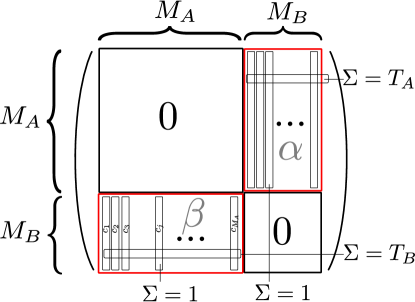
Figure 3: The connectivity matrix of a 2-thermal graph for a D-B process, where nodes of type $A$ are numbered from 1 to $M_{A}$ and nodes of type $B$ from $M_{A}+1$ to $M_{A}+M_{B}$. For a B-D process, the sum of the elements of a row is equal to unity, and the sum of the elements of a column is equal to $T_{A}$ or $T_{B}$.

and all the elements of $\alpha$ block are equal to $1$. Therefore $T_{A}=M_{B}$ and $T_{B}=1/M_{B}$. The star graph can be generalized to the case where the number of central nodes $M_{A}>1$ (figure 2a). For a general bithermal graph the number of $B$ nodes to which an $A$ node connects and the weights of these links can be arbitrary, as long as the constraints on temperatures are respected. Note that $T_{A}$ and $T_{B}$ are not independent. By summing over all the elements $m_{ki}$ of the $\beta$ or $\alpha$ block of the connectivity matrix $\mathbf{m}$, we have for a D-B process

$$M_{A}=M_{B}T_{B}\,\,;\,\,M_{B}=M_{A}T_{A}$$

for a B-D process, the role of $M_{A}$ and $M_{B}$ are exchanged, but in both cases, we have

$$T_{A}T_{B}=1$$ (16)

We now search for the bithermal graphs which have an exact fixed point. Following the example of the isothermal graphs, we look for a fixed point $\boldsymbol{\zeta=}(\zeta_{1},...\zeta_{M})$ where $\zeta_{i}=\zeta_{A}$ if $i\in A$ and $\zeta_{i}=\zeta_{B}$ if $i\in B$ .

Let us first consider the case of D-B processes. Using condition (14) for $k\in A\,\mbox{or}\,B$ we obtain a set of two algebraic equations :

$$f_{A}(\boldsymbol{\zeta}) = \zeta_{A}(\zeta_{B}-1)T_{A}-r^{-1}(\zeta_{A}-1)=0$$

$$f_{B}(\boldsymbol{\zeta}) = \zeta_{B}(\zeta_{A}-1)T_{B}-r^{-1}(\zeta_{B}-1)=0$$

the solution of which is given by

$$\zeta_{A} = u(r,M_{A}/M_{B})$$ (17)

$$\zeta_{B} = u(r,M_{B}/M_{A})$$ (18)

$$u(r,T) = \frac{1/r+T}{r+T}$$ (19)

This solution also satisfies condition (15) if for $k\in A$ and $i\in B$, we have the following relation between the coefficient of the connectivity matrix $\mathbf{m}$ :

$$\frac{m_{ki}}{m_{ik}} = -\frac{(\zeta_{B}-1)(\zeta_{B}-r^{-1})\zeta_{A}}{(\zeta_{A}-1)(\zeta_{A}-r^{-1})\zeta_{B}}$$

$$= \frac{1}{T_{A}}=\frac{M_{A}}{M_{B}}$$

which we can express as a relation between the two blocks $\beta$ and $\alpha$ of the connectivity matrix $\mathbf{m}$:

$$\alpha=T_{A}\beta^{\intercal}$$ (20)

We observe here that this is the sufficient condition to form exactly solvable bithermal graphs : form an $M_{B}\times M_{A}$ matrix $\beta$ where the sum of elements in each column is 1 and the sum of elements in each row is $1/T_{A}=M_{A}/M_{B}$; form the block matrix $\mathbf{m}$ from $\beta$ and $\alpha=T_{A}\beta^{\intercal}$. The $\beta$ block contains $M_{A}M_{B}$ coefficients subject to $M_{A}+M_{B}$ summation rules, so the number of bithermal graphs with exact solutions is indeed very large when $M_{A}$ or $M_{B}$ are large.

An important subset of bithermal graphs that always has an exact fixed point is a set we call symmetric bithermal graphs. For these graphs, all the existing links from a node $A$ to a node $B$ (respect. $B$ to $A$ ) have the same weight $m_{AB}$ (resp. $m_{BA}$). The generalized star graph (fig 2a) belongs to this subset. For these sets, the weight of a link is determined only by the number of connected nodes, and each $A$ (resp. $B$) node has always the same number of neighbors. The symmetric subset automatically satisfies all the constraints and always has exact fixed points.

Once the fixed point is known, the fixation probability is easily determined from equation (13):

$$\pi_{f}=\frac{1-(M_{A}\zeta_{A}+M_{B}\zeta_{B})/(M_{A}+M_{B})}{1-\zeta_{A}^{M_{A}}\zeta_{B}^{M_{B}}}$$ (21)

For a B-D process, the computation of the fixed point follows exactly the same line of argument. The result is obtained by permuting $M_{A}$ and $M_{B}$ :

$$\zeta_{A}^{\mbox{BD}} = u(r,M_{B}/M_{A})\,\,;\,\,\zeta_{B}^{\mbox{BD}}=u(r,M_{A}/M_{B})$$ (22)

The fixation probability is given by the same expression (21). Note that D-B and B-D processes act in opposite directions. Compared to a non-structured population of the same size, a bithermal D-B process acts as a suppressor of selection, lowering the fixation probability where the B-D process is an amplifier of selection, increasing the fixation probability. The maximum $\pi_{f}$ for a D-B is obtained for $T_{A}=1$ and is equal to expression (1) ; the maximum $\pi_{f}$ for a B-D process is obtained for $T_{A}\rightarrow\infty$ and is equal to $1-r^{-2}$. A plot of both fixation probabilities and their comparison to numerical simulations is shown in figure 4

Figure 4: Fixation probability $\pi_{f}$ of bithermal EGs of size $M=100$ and $r=1.25$. (a) $\pi_{f}$ as a function of the number $M_{A}$ of nodes of type $A$ for a generalized ($M_{A},M_{B})$ star. circles (black) and triangles (red) correspond to numerical resolution of the fixation probabilities for B-D and D-B processes. Solid lines correspond to exact solutions given by equation (21). The dashed lines correspond to $\pi_{f}=1-1/r$ and $\pi_{f}=1-1/r^{2}$. Numerical simulations were performed by using a Gillespie Algorithm(Gillespie [4]) ; for each point, $10^{5}$ stochastic paths were generated and used to compute the fixation probability. (b)Fixation probability $\pi_{f}$ for random bithermal EG for different values of $M_{A}$ (circles 5, squares 10, $\times$ 15, diamond 20, triangle up 30,triangle down 45) and D-B processes. To the left of the vertical line (#index $\leq$50) : Each point corresponds to a random bithermal connectivity matrix where the two blocks are related through $\alpha=T_{A}\beta^{\intercal}$. To the right of the vertical line (#index >50) : For each point, the two blocks of the bithermal connectivity matrix are random and $\alpha\neq T_{A}\beta^{\intercal}$. Solid lines indicate the theoretical values computed by equation (21).

.

We stress that for bithermal graphs, the details of the connectivity are not important : the fixation probability depends only on the total number of $A$ and $B$ nodes. Consider for example the symmetric generalized star $(M_{A},M_{B},p,q)$ where each $A$ node is connected to $p$ nodes of type $B$ and each $B$ nodes to $q$ nodes of type $A$. For a fully connected generalized star, $p=M_{B}$ and $q=M_{A}$ ; an example of partially connected generalized star is given in figure 2a. We emphasize that for generalized stars, the fixation probability does not depend on the detail of the connectivity $p,q$, a result which would be hard to predict by other methods. We also note from numerical simulations that the fixation time is also only a function of $M_{A}$ and $M_{B}$ and does not depend on the detail of the connectivity.

Finally, we note that even when the constraint (20) is not respected and $\alpha\neq T_{A}\beta^{\intercal}$, the fixation probability of bithermal graphs is well approximated by expression (21). In this case, the point $\boldsymbol{\zeta}$ computed from equations (17,18) is only a quasi-fixed point, but as we have shown earlier(Houchmandzadeh and Vallade [6]), for large communities, quasi-fixed points can be used for a good approximation of the fixation probability. It can be observed in figure (4b) that the numerical errors of fixation probabilities of connectivity matrices having exact fixed points (left of vertical line) or only quasi-fixed point (right of vertical line) are of the same magnitude, for a system as small as $M=100$. We also note from numerical simulations that fixation time, is only

5 Discussion and Conclusion.

The approach we presented above can be generalized in various directions. We have restricted our approach to the case where each node contains only one individual. This restriction can be relaxed and we can let each node contain a number of individuals $N\geq 1$ (figure 5)

Figure 5: Generalization to bi-level graphs, where each node can be considered as composed of $N$ individuals, conserving the same topology, i.e. the weight of new links is downscaled by a factor $N$ : $m^{\prime}_{ij}=m_{ij}/N$

. This is equivalent to the original island model of Maruyama(Maruyama [9]) or can alternatively be envisioned as a bi-level graph as defined by Shakarian et al(Shakarian et al. [13]), where each node is mapped into $N$ sub-nodes conserving the original topology. As we have shown earlier(Houchmandzadeh and Vallade [6]), this parameter does not alter the expression of the PGF and the fixed points are still computed by the same equations. The fixation probability is slightly modified and reads

$$\pi_{f}=\frac{1-(M_{A}\zeta_{A}+M_{B}\zeta_{B})/(M_{A}+M_{B})}{1-\zeta_{A}^{NM_{A}}\zeta_{B}^{NM_{B}}}$$

The approach can be extended even further and allows for different numbers $N_{k}$ of individuals for each node $k$ (Houchmandzadeh and Vallade [6]).

Another direction toward which this work can be extended is the $n-$thermal graphs. Here we have considered only bithermal graphs composed of two types of nodes which we can represent by an $A-B$ topology. In principle, we can generalize the method to graphs containing $P$ types of nodes $O_{1},...,O_{P}$ : The $M_{I}$ nodes belonging to type $O_{I}$ have the temperature $T_{I}$ and a hot class can only be connected to cold classes and vice versa. We could in principle form a polymeric topology such as $O_{1}-O_{2}...-O_{P}$, branched systems, closed rings and so on. The exploration of these topologies implies an analytic study of the roots of algebraic equations of order $2P$ and is beyond the scope of the present article.

To summarize, we have obtained exact analytical results for a wide class of graphs that we have called bithermal in the field of Evolutionary Graph Theory. EGT is a cornerstone for our understanding of evolution, because natural population are always geographically extended and cannot be a priori approximated as “well mixed”. Exact results in EGT however have been hard to obtain because in each case, a mapping into a one-dimensional Brownian motion has to be constructed ; whether such a mapping exists or not for a particular problem is not a trivial problem. The method we develop is radically different : by using the continuous time version of the Moran model and the dynamics of the PGF, we reduce the problem of finding an exactly solvable model into finding the roots of algebraic equations. We have illustrated the power of this dynamical method through our study of bithermal graphs. We believe that the method we have presented can be a powerful tool to get exact results for the fixation probability of more complex evolutionary graphs.

Acknowledgements.

We are grateful to E. Geissler and O. Rivoire for the careful reading of the manuscript and fruitful discussions. This work was partly funded by Agence Nationale de la Recherche Française (ANR) grant “Evo-Div.”

References

- Antal et al. [2006] Antal, T., Redner, S., Sood, V., 2006. Evolutionary dynamics on degree-heterogeneous graphs. Phys Rev Lett 96 (18), 188104.
- Barbosa et al. [2010] Barbosa, V. C., Donangelo, R., Souza, S. R., 2010. Early appraisal of the fixation probability in directed networks. Phys Rev E 82, 046114.
- Ewens [2004] Ewens, W. J., 2004. Mathematical Population Genetics. Springer-Verlag.
- Gillespie [1977] Gillespie, D. T., 1977. Exact stochastic simulation of coupled chemical reactions. The Journal of Physical Chemistry 81, 2340–2361.
- Houchmandzadeh and Vallade [2010] Houchmandzadeh, B., Vallade, M., 2010. Alternative to the diffusion equation in population genetics. Phys Rev E Stat 82, 051913.
- Houchmandzadeh and Vallade [2011] Houchmandzadeh, B., Vallade, M., 2011. The fixation probability of a beneficial mutation in a geographically structured population. New J. Physics 13, 073020.
- Kimura [1962] Kimura, M., 1962. On the probability of fixation of mutant genes in a population. Genetics 47, 713–719.
- Lieberman et al. [2005] Lieberman, E., Hauert, C., Nowak, M. A., 2005. Evolutionary dynamics on graphs. Nature 433, 312–316.
- Maruyama [1974a] Maruyama, T., 1974a. A markov process of gene frequency change in a geographically structured population. Genetics 76, 367–377.
- Maruyama [1974b] Maruyama, T., 1974b. A simple proof that certain quantities are independent of the geographical structure of population. Theor Popul Biol 5, 148–154.
- Moran [1962] Moran, P., 1962. The Statistical processes of of evolutionary theory. Oxford University Press.
- Patwa and Wahl [2008] Patwa, Z., Wahl, L. M., 2008. The fixation probability of beneficial mutations. J R Soc Interface 5, 1279–1289.
- Shakarian et al. [2012] Shakarian, P., Roos, P., Johnson, A., 2012. A review of evolutionary graph theory with applications to game theory. Biosystems 107, 66–80.