We consider a weakly coupled gauge theory where charged particles all have large gaps (ie no Higgs condensation to break the gauge “symmetry”) and the field strength fluctuates only weakly. We ask, what kind of topological terms (the terms that do not depend on space-time metrics) can be added to the Lagrangian of such a weakly coupled gauge theory. For example, for weakly coupled $U(1)$ gauge theory in $d=3$ space-time dimensions, a Chern-Simons topological term $\frac{k}{4\pi}a_{\mu}\partial_{\nu}a_{\lambda}\epsilon^{\mu\nu\lambda},\ k\in\mathbb{Z}$ can be added.

In this paper, we systematically construct quantized topological terms which are generalization of the Chern-Simons terms and $F\wedge F$ terms, in any space-time dimensions and for any gauge groups (continuous or discrete). We can use each element of the topological cohomology classes $H^{d+1}(BG,\mathbb{Z})$ on the classifying space $BG$ of the gauge group $G$ to construct a quantized topological term in $d$ space-time dimensions.

In 3$d$ or for finite gauge groups above 3$d$, the weakly coupled gauge theories are gapped. So our results on topological terms can be viewed as a systematic construction of gapped topologically ordered phases of weakly coupled gauge theories. In other cases, the weakly coupled gauge theories are gapless. So our results can be viewed as an attempt to systematically construct different gapless phases of weakly coupled gauge theories.

Amazingly, the bosonic symmetry protected topological (SPT) phases with a finite on-site symmetry group $G$ are also classified by the same $H^{d+1}(BG,\mathbb{Z})$. (SPT phases are gapped quantum phases with a symmetry and trivial topological order.) In this paper, we show an explicit duality relation between topological gauge theories with the quantized topological terms and the bosonic SPT phases, for any finite group $G$ and in any dimensions; a result first obtained by Levin and Gu. We also study the relation between topological lattice gauge theory and the string-net states with non-trivial topological order and no symmetry.

Quantized topological terms in weakly coupled gauge theories
and their connection to symmetry protected topological phases

I Introduction

Quantum many-body systems can be described by Lagrangians in space-time. As we change the coupling constants in a Lagrangian a little, the new Lagrangian will describe a new quantum many-body system which is usually in the same phase as the original system. However, the Lagrangians may also contain the so called topological terms – the terms that do not depend on space-time metrics. Some of those topological terms are quantized. Adding quantized topological terms to a Lagrangian will generate new Lagrangians that usually describe different phases of quantized many-body systems.

So studying and classifying quantized topological terms is one way to understand and classify different possible phases of quantum many-body systems. For example, a non-linear $\sigma$-model

$${\cal L}=\frac{1}{\lambda}[\partial g(x^{\mu})]^{2},\ \ g\in G$$ (1)

with symmetry group $G$ can be in a disordered phase that does not break the symmetry $G$ when $\lambda$ is large. By adding different $2\pi$ quantized topological $\theta$-terms to the Lagrangian ${\cal L}$, we can get different Lagrangians that describe different disordered phases that does not break the symmetry $G$.Chen et al. (2011a) Those disordered phases are the symmetry protected topological (SPT) phases.Gu and Wen (2009); Pollmann et al. (2009) We find that the different $2\pi$ quantized topological $\theta$-terms in $d$-dimensional space-time can be classified by the Borel group cohomology classes ${\cal H}^{d}_{B}(G,\mathbb{R}/\mathbb{Z})$, which leads us to believe that the SPT phases in $d$-dimensional space-time can be classified by ${\cal H}^{d}_{B}(G,\mathbb{R}/\mathbb{Z})$.Chen et al. (2011b, a) So the possible topological terms in a non-linear $\sigma$-model help us to understand the possible phases of the non-linear $\sigma$-model.

This motivated us to study possible quantized topological terms in gauge theory, hoping to understand different phases of gauge theory in a more systematic way. But a gauge theory is a very complicated system whose low energy phases can be any thing. To make our problem better defined, we need to restrict ourselves to a special class of gauge theories that we will call “weakly coupled gauge theories” or “weakly coupled lattice gauge theories”. “Weakly coupled (lattice) gauge theories”, by definition, are lattice gauge theories in the weak coupling limit (where gauge flux through each plaquette is small) and all the gauge charged excitations have a large energy gap (ie no Higgs condensations).

We find that a quantized topological term in the weakly coupled gauge theories can be constructed from each element in topological cohomology class $H^{d+1}(BG,\mathbb{Z})$ for the classifying space $BG$ of the gauge group $G$ in $d$ space-time dimensions.

The result is obtained by applying the three approaches introduced by Baker and by Dijkgraaf and WittenBaker (1977); Dijkgraaf and Witten (1990) to lattice gauge theories.

In the first approach (see section II), we follow Dijkgraaf and WittenDijkgraaf and Witten (1990) to use cocycles in group cohomology class ${\cal H}^{d}_{B}(G,\mathbb{R}/\mathbb{Z})$ to construct topological terms in weakly coupled gauge theories in $d$-dimensional space-time with a finite gauge group $G$. Such weakly coupled gauge theories are gapped and describe topological phases. So we can use ${\cal H}^{d}_{B}(G,\mathbb{R}/\mathbb{Z})$ to describe different topological phases in weakly coupled gauge theories with finite gauge group.

In the second approach (see section III), we view a lattice gauge theory as a lattice non-linear $\sigma$-model whose target space is given by the classifying space $BG$ of the gauge group $G$. So the quantized topological terms in a weakly coupled lattice gauge theory can be described by the quantized topological terms in the non-linear $\sigma$-model of the classifying space $BG$. Such a quantized topological term is similar to the one used in the classification of SPT phases,Chen et al. (2011a); Gu and Wen (2012) where the target space is simply the symmetry group $G$. Using this approach, we find that some quantized topological terms in weakly coupled gauge theories with gauge group $G$ can be constructed from the torsion elements in topological cohomology class $\text{Tor}[H^{d+1}(BG,\mathbb{Z})]$ of the classifying space $BG$. Since ${\cal H}_{B}^{d}(G,\mathbb{R}/\mathbb{Z})=H^{d+1}(BG,\mathbb{Z})=\text{Tor}[H^{d+1}(BG,\mathbb{Z})]$ for finite groups,Chen et al. (2011a) the second approach contains the result of the first approach.

In the third approach (see section IV), we express $d$-dimensional Chern-Simons terms (assuming $d$ = odd) in terms of the differential characters of Chern, Simons and Cheeger.Baker (1977); Dijkgraaf and Witten (1990) The different differential characters are classified by $H^{d+1}(BG,\mathbb{Z})$,Baker (1977) thus in turn giving a classification of Chern-Simons terms with gauge group $G$. We see that the quantized topological terms obtained from the third approach (classified by $H^{d+1}(BG,\mathbb{Z})$) contain those obtained from the second approach (classified by $\text{Tor}[H^{d+1}(BG,\mathbb{Z})]$), in $d$ = odd space-time dimensions.

Also, in $d=$ even space-time dimensions, $H^{d+1}(BG,\mathbb{Z})=\text{Tor}[H^{d+1}(BG,\mathbb{Z})]$ (see eqn. (95)). So the quantized topological terms are classified by $H^{d+1}(BG,\mathbb{Z})$ in any dimensions. Since

$${\cal H}_{B}^{d}(G,\mathbb{R}/\mathbb{Z})\simeq H^{d+1}(BG,\mathbb{Z})$$ (2)

[see eqn. (J32) in Ref. Chen et al., 2011a], this suggests that the quantized topological terms in weakly coupled gauge theories are described by ${\cal H}_{B}^{d}(G,\mathbb{R}/\mathbb{Z})$. Here $G$ can be a continuous group. Thus the quantized topological terms is the dual of the SPT phases classified by the same ${\cal H}^{d}_{B}(G,\mathbb{R}/\mathbb{Z})$.

We know that, for continuous gauge group $G$, a kind of quantized topological terms – Chern-Simons terms – can be defined in any $d$ = odd dimensions:

$$S_{3d} =\int_{M}\frac{2\pi K}{2!(2\pi)^{2}}{\rm Tr}(AF-\frac{A^{3}}{3})+\frac{F_{\mu\nu}F^{\mu\nu}}{\lambda},$$

$$S_{5d} =\int_{M}\frac{2\pi K}{3!(2\pi)^{3}}{\rm Tr}(AF^{2}-\frac{A^{3}F}{2}-\frac{A^{5}}{10})+\frac{F_{\mu\nu}F^{\mu\nu}}{\lambda},$$

$$......$$ (3)

where $K$ = integer, $A$ is the gauge potential one form and $F$ the gauge field strength two form. Also, for example, $AF^{2}$ means the wedge product $A\wedge F\wedge F$. We have also included the usual kinetic term in the above with coefficient $1/\lambda$. In $d=3$ space-time dimensions, a Chern-Simons gauge theory is gapped and describes a topologically ordered phase. So the topological phases of a $d=3$ weakly coupled gauge theory are described by ${\cal H}_{B}^{3}(G,\mathbb{R}/\mathbb{Z})$. Beyond $d=3$, the above Chern-Simons gauge theory is gapless for small $\lambda$, and the Chern-Simons term is irrelevant at low energies. However, the Chern-Simons term is not renormalized, and we believe that different Chern-Simons terms will describe different gapless phases of the weakly coupled gauge theory. Consider $d=5$ $U(1)$ Chern-Simons theory, if the space-time has a topology of $M^{3}\times S^{2}$ and the $U(1)$ gauge field has a non-zero total flux through $S^{2}$, the $d=5$ $U(1)$ Chern-Simons theory on $M^{3}\times S^{2}$ will becomes a non-trivial $d=3$ $U(1)$ Chern-Simons theory on $M^{3}$ which describes a non-trivial topological phase.

The above discussion is for $d$ = odd dimensions. Similarly, in $d$ = even space-time dimensions, we can have the following weakly coupled gauge theories with topological term

$$S_{4d} =\int_{M}\frac{\theta}{2!(2\pi)^{2}}{\rm Tr}(F^{2})+\frac{F_{\mu\nu}F^{\mu\nu}}{\lambda},$$

$$S_{6d} =\int_{M}\frac{\theta}{3!(2\pi)^{3}}{\rm Tr}(F^{3})+\frac{F_{\mu\nu}F^{\mu\nu}}{\lambda},$$

$$......$$ (4)

where $\theta\in[0,2\pi)$ and $\lambda$ is small.

The above topological terms are not quantized and do not give rise to new phases. In this paper, we show that quantized topological terms do exist for weakly coupled gauge theories in $d=$ even space-time dimensions. Such quantized topological terms are described by $H^{d+1}(BG,\mathbb{Z})=$ Tor$[H^{d+1}(BG,\mathbb{Z})]$. Again, the quantized topological terms do not open a mass gap in $d\geq 6$ dimensional space-time (for small $\lambda$). Here we like to propose that the different quantized topological terms give rise to different gapless phases of the gauge theories. The situation is even more interesting (and unclear) in $d=4$ dimensional space-time, where some gauge theories are confined even in small $\lambda$ limit. It is not clear if the different quantized topological terms give rise to different confined phases.

Since the introduction of topological order in 1989,Wen (1989, 1990) we have introduced many ways of constructing topologically ordered states (ie long range entangled states) on lattice: resonating-valence-bond state,Rokhsar and Kivelson (1988); Moessner and Sondhi (2003) projective construction,Baskaran et al. (1987); Affleck et al. (1988); Dagotto et al. (1988); Wen et al. (1989); Read and Sachdev (1991); Wen (1991, 1999) string-net condensation,Freedman et al. (2004); Levin and Wen (2005); Chen et al. (2010); Gu et al. (2010) weakly coupled gauge theory of finite gauge group, etc .

The usual construction of weakly coupled lattice gauge theories for a given finite gauge group only gives rise to one type of topological order. In this paper, we manage to “twist” the weakly coupled gauge theory with a given finite gauge group by adding topological terms to obtain more general topological orders. The added topological terms are constructed from ${\cal H}_{B}^{d}(G,\mathbb{R}/\mathbb{Z})=H^{d+1}(BG,\mathbb{Z})$ (see table 1).

group $G$	$d=1$	$d=2$	$d=3$	$d=4$
$Z_{n}$	$\mathbb{Z}_{n}$	$0$	$\mathbb{Z}_{n}$	$0$
$Z_{m}\times Z_{n}$	$\mathbb{Z}_{m}\oplus\mathbb{Z}_{n}$	$\mathbb{Z}_{(m,n)}$	$\mathbb{Z}_{m}\oplus\mathbb{Z}_{n}\oplus\mathbb{Z}_{(m,n)}$	$\mathbb{Z}^{2}_{(m,n)}$
$Z_{n}\rtimes Z_{2}$	$\mathbb{Z}_{2}\oplus\mathbb{Z}_{(2,n)}$	$\mathbb{Z}_{(2,n)}$	$\mathbb{Z}_{n}\oplus\mathbb{Z}_{2}\oplus\mathbb{Z}_{(2,n)}$	$\mathbb{Z}^{2}_{(2,n)}$
$U(1)$	$\mathbb{Z}$	$0$	$\mathbb{Z}$	$0$
$U(1)\rtimes Z_{2}$	$\mathbb{Z}_{2}$	$\mathbb{Z}_{2}$	$\mathbb{Z}\oplus\mathbb{Z}_{2}$	$\mathbb{Z}_{2}$
$U(1)\times Z_{2}$	$\mathbb{Z}\oplus\mathbb{Z}_{2}$	$0$	$\mathbb{Z}\oplus\mathbb{Z}^{2}_{2}$	$0$
$U(1)\times U(1)\rtimes Z_{2}$	$\mathbb{Z}_{2}\oplus\mathbb{Z}$	$\mathbb{Z}_{2}$	$\mathbb{Z}^{2}\oplus\mathbb{Z}_{2}^{2}$	$\mathbb{Z}_{2}^{2}$
$SU(2)$	$0$	$0$	$\mathbb{Z}$	$0$
$SO(3)$	$0$	$\mathbb{Z}_{2}$	$\mathbb{Z}$	$0$

Table 1: The above table lists ${\cal H}_{B}^{d}[G,\mathbb{R}/\mathbb{Z}]=H^{d+1}[G,\mathbb{Z}]$ whose elements label the quantized topological terms of weakly coupled lattice gauge theories with gauge group $G$ in $d$ space-time dimensions. Here $0$ means that our construction only gives rise to a trivial topological term which is zero. $\mathbb{Z}_{n}$ means that the constructed non-trivial topological terms plus the trivial one are labeled by the elements in $\mathbb{Z}_{n}$. $\mathbb{Z}_{n}^{2}$ means $\mathbb{Z}_{n}\oplus\mathbb{Z}_{n}$. $U(1)$ represents $U(1)$ symmetry, $Z_{n}$ represents cyclic symmetry, etc . Also $(m,n)$ is the greatest common divisor of $m$ and $n$.

We also manage to “twist” the weakly coupled gauge theory of continuous gauge group by adding topological terms. The added topological terms in this case are constructed from $H^{d+1}(BG,\mathbb{Z})={\cal H}_{B}^{d}(G,\mathbb{R}/\mathbb{Z})$. This leads to more general topological orders in (2+1)D than those described by the standard Chern-Simons terms. But in higher dimensions, this may lead to more general gapless phases of weakly coupled gauge theories (see table 1).

From Ref. Randal-Williams, 2011, we find that $H^{7}(U(1)\rtimes Z_{2},\mathbb{Z})=\mathbb{Z}_{2}\oplus\mathbb{Z}_{2}$. So there are three non-trivial quantized topological terms that we can add to the $U(1)\rtimes Z_{2}$ weakly coupled gauge theory in $6$-dimensional space-time. We think that one of the quantized topological term is given by

$$S_{U(1)\rtimes Z_{2}} =\int_{M}\frac{\theta}{3!(2\pi)^{3}}F\wedge F\wedge F+\frac{(F_{\mu\nu})^{2}}{\lambda},\ \ \theta=\pi$$ (5)

where $F$ is the field strength of the $U(1)$ gauge field and the $Z_{2}$ gauge transformation acts as $F\to-F$.Bucher et al. (1992) Such a $U(1)\rtimes Z_{2}$ gauge theory can be viewed as the $U(1)$ gauge theory with the $Z_{2}$ gauged charge conjugation symmetry. Note that the theory has a charge conjugation symmetry only when $\theta=0,\pi$.

The gapless phases (in small $\lambda$ limit) for $\theta=0$ and $\theta=\pi$ should be different.

Similarly, we can have a quantized topological term in $U(1)\times U(1)\rtimes Z_{2}$ weakly coupled gauge theory in $4$-dimensional space-time:

$$S_{U(1)\times U(1)\rtimes Z_{2}} =\int_{M}\frac{\theta}{(2\pi)^{2}}\tilde{F}\wedge F+\frac{(F_{\mu\nu})^{2}}{\lambda}+\frac{(\tilde{F}_{\mu\nu})^{2}}{\lambda},$$ (6)

where $\theta=\pi$, $F,\tilde{F}$ are the field strengthes of the two $U(1)$ gauge fields and the $Z_{2}$ gauge transformation acts as $F\to-F$. In such a $U(1)\times U(1)\rtimes Z_{2}$ gauge theory, the $U(1)\times U(1)$ magnetic monopole with monopole charge $(m,\tilde{m})$ will carry electric charges $(q,\tilde{q})=(\frac{\tilde{m}\theta}{2\pi}+\text{int.},\frac{m\theta}{2\pi}+\text{int.})$.Witten (1979); Rosenberg and Franz (2010) We see that when $\theta=\pi$, dyons with quantum numbers $(q,m;\tilde{q},\tilde{m})=(\pm\frac{1}{2},\pm 1;\pm\frac{1}{2},\pm 1)$ all appear, which is consistent with the $Z_{2}$ gauge symmetry.

When $\theta=0$, a dyon with quantum number $(q,m;\tilde{q},\tilde{m})$ has a statistics $(-)^{qm+\tilde{q}\tilde{m}}$ (where $+$ means Bose statistics and $-$ means Fermi statistics and note that $q$, $\tilde{q}$, $m$ and $\tilde{m}$ are all integers).Tamm (1931); Jackiw and Rebbi (1976); Wilczek (1982); Goldhaber (1982); Lechner and Marchetti (2000) It is shown in Ref. Goldhaber et al., 1989 that the statistics of a dyon in the presence of the $F\wedge\tilde{F}$ term does not depend on $\theta$. So for a non-zero $\theta$, the satistics is given by

$$(-)^{(q-\frac{\tilde{m}\theta}{2\pi})m+(\tilde{q}-\frac{m\theta}{2\pi})\tilde{m}}=(-)^{qm+\tilde{q}\tilde{m}-\frac{\theta}{\pi}m\tilde{m}}$$ (7)

where the electric charges $q,\ \tilde{q}$ are no longer integers: $q=\frac{\tilde{m}\theta}{2\pi}$ + integer and $\tilde{q}=\frac{m\theta}{2\pi}$ + integer. We see that when $\theta=\pi$, the statistics is invariant under the $Z_{2}$ gauge transformation $(q,m;\tilde{q},\tilde{m})\to(-q,-m;\tilde{q},\tilde{m})$. A $(q,m;\tilde{q},\tilde{m})=(\frac{1}{2},1;\frac{1}{2},1)$ dyon is a boson while a $(q,m;\tilde{q},\tilde{m})=(\frac{1}{2},1;-\frac{1}{2},1)$ dyon is a fermion. Clearly, the $\theta=0$ and $\theta=\pi$ correspond to two different gapless phases of the $U(1)\times U(1)\rtimes Z_{2}$ gauge theory in $4$ space-time dimensions.

It is amazing to see that the $d$-dimensional SPT phases and the $d$-dimensional quantized topological terms in weakly coupled gauge theories are classified by the same thing ${\cal H}_{B}^{d}(G,\mathbb{R}/\mathbb{Z})=H^{d+1}(BG,\mathbb{Z})$. In this paper, we would like to clarify a duality relation between the $d$-dimensional SPT phase and $d$-dimensional topological gauge theory for finite groups (see section V). (Here a topological gauge theory with a finite gauge group is defined as a weakly coupled gauge theory with a finite gauge group and a quantized topological term.) Such a duality relation is exactly the duality relation first proposed by Levin and Gu in 3-dimensions.Levin and Gu (2012) We know that the SPT phases are described by topological non-linear $\sigma$-models with symmetry $G$:

$${\cal L}=\frac{1}{\lambda_{s}}[\partial g(x^{\mu})]^{2}+\hskip 1.0pt\mathrm{i}\hskip 1.0ptW_{\text{top}}(g),\ \ g\in G$$ (8)

where the $2\pi$-quantized topological term $\int W_{\text{top}}(g)$ is classified by ${\cal H}_{B}^{d}(G,\mathbb{R}/\mathbb{Z})$ which describes different SPT phases. If we “gauge” the symmetry $G$, the topological non-linear $\sigma$-model will become a gauge theory:

$${\cal L}=\frac{1}{\lambda_{s}}[(\partial-\hskip 1.0pt\mathrm{i}\hskip 1.0ptA)g(x^{\mu})]^{2}+\hskip 1.0pt\mathrm{i}\hskip 1.0ptW_{\text{top}}(g,A)+\frac{(\tilde{F}_{\mu\nu})^{2}}{\lambda}.$$ (9)

If we integrate out $g$, we will get a pure gauge theory with a topological term

$${\cal L}=\frac{(\tilde{F}_{\mu\nu})^{2}}{\lambda}+\hskip 1.0pt\mathrm{i}\hskip 1.0pt\tilde{W}_{\text{top}}(A).$$ (10)

This line of thinking suggests that the gauge-theory topological term $\int\tilde{W}_{\text{top}}(A)$ is classified by ${\cal H}_{B}^{d}(G,\mathbb{R}/\mathbb{Z})$. Since ${\cal H}_{B}^{d}(G,\mathbb{R}/\mathbb{Z})=H^{d+1}(BG,\mathbb{Z})$, the topological terms constructed this way agrees with the topological terms constructed through the classifying space, which realizes the duality relation.

We remark that the SPT phases are described by topological non-linear $\sigma$-models with symmetry $G$. If we “gauge” the symmetry $G$, the topological non-linear $\sigma$-model will become a gauge theory– a principal chiral model,Liu and Wen (2012); Chen and Wen (2012) which realizes the duality relation.

II Lattice topological gauge theory

II.1 Discretize space-time

In this paper, we will consider gauge theories on discrete space-time which are well defined. We will discretize the space-time $M$ by considering its triangulation $M_{\text{tri}}$ and define the $d$-dimensional topological gauge theory on such a triangulation. We will call such a theory a lattice topological gauge theory. We will call the triangulation $M_{\text{tri}}$ a space-time complex, and a cell in the complex a simplex.

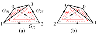
Figure 1: (Color online) Two branched simplices with opposite orientations. (a) A branched simplex with positive orientation and (b) a branched simplex with negative orientation.

In order to define a generic lattice theory on the space-time complex $M_{\text{tri}}$, it is important to give the vertices of each simplex a local order. A nice local scheme to order the vertices is given by a branching structure.Costantino (2005); Chen et al. (2011a) A branching structure is a choice of orientation of each edge in the $d$-dimensional complex so that there is no oriented loop on any triangle (see Fig. 1).

The branching structure induces a local order of the vertices on each simplex. The first vertex of a simplex is the vertex with no incoming edges, and the second vertex is the vertex with only one incoming edge, etc . So the simplex in Fig. 1a has the following vertex ordering: $0,1,2,3$.

The branching structure also gives the simplex (and its sub simplexes) an orientation. Fig. 1 illustrates two $3$-simplices with opposite orientations. The red arrows indicate the orientations of the $2$-simplices which are the subsimplices of the $3$-simplices. The black arrows on the edges indicate the orientations of the $1$-simplices.

II.2 Lattice gauge theory on a branched space-time complex – finite gauge group

Now, we are ready to define lattice gauge theory on a branched space-time complex. We first choose a gauge group $G$. For the time being, let us assume that $G$ is finite. We then assign $G_{ij}\in G$ to each link $ij$ in the space-time complex $M_{\text{tri}}$, where $i\to j$ is the orientation of the link. For each simplex (with vertices $i,j=0,1,...$), we assign a complex action amplitude $\alpha(\{G_{ij}\})$.

The imaginary-time path integral of the lattice gauge theory is given by

$$Z={\sum_{\{G_{ij}\}}}^{\prime}\prod_{[ij...k]}\alpha^{s(i,j,...,k)}(\{G_{ij}\}),$$ (11)

where $\prod_{[ij...k]}$ is the product over all the simplices $[ij...k]$ in the space-time complex $M_{\text{tri}}$, and $s(i,j,...,k)=1$ or ${\dagger}$ depending on the orientation of the simplex $[ij...k]$ defined by the branching structure. Two sets $\{G_{ij}\}$ and $\{G^{\prime}_{ij}\}$ are said to be gauge equivalent if there exists a set $g_{i}\in G$, such that

$$G^{\prime}_{ij}=g_{i}G_{ij}g_{j}^{-1}.$$ (12)

We require the above lattice theory to be gauge invariant:

$$\prod_{[ij...k]}\alpha^{s(i,j,...,k)}(\{g_{i}G_{ij}g_{j}^{-1}\}) =\prod_{[ij...k]}\alpha^{s(i,j,...,k)}(\{G_{ij}\}),$$

$$\forall g_{i} \in G,$$ (13)

for any closed space-time complex $M_{\text{tri}}$: $\partial M_{\text{tri}}=\emptyset$. In eqn. (11), ${\sum}^{\prime}_{\{G_{ij}\}}$ sums over the gauge equivalent classes of $\{G_{ij}\}$. This way, we define a lattice gauge theory with gauge group $G$. We may rewrite the path integral as

$$Z=|G|^{-N_{v}}\sum_{\{G_{ij}\}}\prod_{[ij...k]}\alpha^{s(i,j,...,k)}(\{G_{ij}\}),$$ (14)

where $|G|$ is the number of elements in $G$, $N_{v}$ the number of vertices. The overall normalization factor can be understood as modding out the theory by its overall redundant phase volume.

II.3 Lattice topological gauge theory – finite gauge group

What is the low energy fixed-point theory of the lattice gauge theory defined above, if the theory is in a gapped phase? In a study of SPT phases, we have discussed the gapped phases of non-linear $\sigma$-model and the related fixed-point theories (or topological theories).Chen et al. (2011a); Gu and Wen (2012) There, the fixed-point theories have the following defining properties, that the action amplitudes for any paths are always equal to 1 if the space-time manifold has a spherical topology. Here we will use the similar idea to study the fixed-point theory of the gapped phases of a lattice gauge theory.

First, one possible low energy fixed-point theory is given by the following action amplitude

$$\alpha(\{G_{ij}\})=1.$$ (15)

Such an action amplitude does not change under the renormalization of the coarse graining and describes a fixed-point theory. However, such a fixed-point theory describes a confined phase with trivial topological order. In this paper, we will regard such a fixed-point theory to have a trivial gauge group.

We would like to ask, is this the only way for a gauge theory to become gapped? Can gauge theory become gapped without confinement and the reduction of gauge group? The answer to the above questions is yes: a gauge theory with a finite gauge group can be gapped even without confinement. So in this section, we will consider gauge theories with a finite gauge group.

Figure 2: Complices with spherical topology: (a) a tetrahedron – a (1+1)D sphere, (b) a pentachoron – a (2+1)D sphere. The arrows on the link represent the branching structure.

The fixed-point action (15) describes a confined phase since the Wilson loop operator, such as $G_{ij}G_{jk}G_{ki}$, can fluctuate strongly. So to obtain a fixed-point theory with the original gauge group $G$, we require that

$$|\alpha(\{G_{ij}\})|=1\ \text{ only when }G_{ij}G_{jk}G_{ki}=1,$$ (16)

on all the triangles of the simplex on which $\alpha(\{G_{ij}\})$ is defined. In other words, the amplitude of a path is zero if there is a non-zero flux $G_{ij}G_{jk}G_{ki}\neq 1$ on some trangles. We will call this condition a flat connection condition since it corresponds to requiring the “field strength $F=0$”. In order for $\alpha(\{G_{ij}\})$ to describe a fixed-point topological theory, we also require that

$$\prod_{[ij...k]}\alpha^{s(i,j,...,k)}(\{G_{ij}\})=1$$ (17)

on all the complex $M_{\text{tri}}$ that have a spherical topology. (It would be too strong to require $\prod_{[ij...k]}\alpha^{s(i,j,...,k)}(\{G_{ij}\})=1$ on any closed complex $M_{\text{tri}}$.)

In (1+1) dimensions, the simplest sphere is a tetrahedron. Due to the flat connection condition, we can use $G_{1}=G_{01}$, $G_{2}=G_{12}$, and $G_{3}=G_{23}$ to label all the $G_{ij}$’s (see Fig. 2a). For example, $G_{02}=G_{1}G_{2}$. On a tetrahedron, the condition (17) becomes

$$\frac{\alpha(G_{1},G_{2})\alpha(G_{1}G_{2},G_{3})}{\alpha(G_{2},G_{3})\alpha(G_{1},G_{2}G_{3})}=1.$$ (18)

We note that if $\alpha(G_{1},G_{2})$ is a solution of the above equation, then $\alpha^{\prime}(G_{1},G_{2})$ defined below is also a solution of the above equation:

$$\alpha^{\prime}(G_{1},G_{2})=\alpha(G_{1},G_{2})\frac{\beta(G_{1})\beta(G_{2})}{\beta(G_{1}G_{2})}.$$ (19)

We regard the two solutions to be equivalent. The equivalent classes of the solutions correspond to different lattice topological gauge theories in (1+1) dimensions.

In (2+1) dimensions, the simplest 3-sphere is a pentachoron. Due to the flat connection condition, we can use $G_{1}=G_{01}$, $G_{2}=G_{12}$, $G_{3}=G_{23}$, and $G_{4}=G_{34}$ to label all the $G_{ij}$’s (see Fig. 2b). For example, $G_{02}=G_{1}G_{2}$. On a tetrahedron, the condition (17) becomes

$$\frac{\alpha(G_{1},G_{2},G_{3})\alpha(G_{1},G_{2}G_{3},G_{4})\alpha(G_{2},G_{3},G_{4})}{\alpha(G_{1}G_{2},G_{3},G_{4})\alpha(G_{1},G_{2},G_{3}G_{4})}=1$$ (20)

We note that if $\alpha(G_{1},G_{2},G_{3})$ is a solution of the above equation, then $\alpha^{\prime}(G_{1},G_{2},G_{3})$ defined below is also a solution of the above equation:

$$\alpha^{\prime}(G_{1},G_{2},G_{3})=\alpha(G_{1},G_{2},G_{3})\frac{\beta(G_{1},G_{2})\beta(G_{1}G_{2},G_{3})}{\beta(G_{2},G_{3})\beta(G_{1},G_{2}G_{3})}.$$ (21)

Again, the above defines an equivalence relation between the solutions. The distinct equivalence classes of the solutions correspond to different lattice topological gauge theories in (2+1) dimensions.

The above discussion can be generalized to any dimensions. We also note that the equivalence class defined above is nothing but the group cohomology class ${\cal H}^{d}(G,\mathbb{R}/\mathbb{Z})$. Therefore, the lattice topological gauge theory with a finite gauge group $G$ is classified by ${\cal H}^{d}(G,\mathbb{R}/\mathbb{Z})$ in $d$ dimensions, a result first obtained by Dijkgraaf and Witten.Dijkgraaf and Witten (1990) From the above discussions, we see that the result can also be phrase in a more physical way: the gapped phases of a lattice gauge theory with a finite gauge group $G$ is classified by ${\cal H}^{d}(G,\mathbb{R}/\mathbb{Z})$ in $d$ space-time dimensions, provided that there is no confinement and the reduction of gauge group (ie the “field strength $F$” fluctuate weakly).

We see that a lattice gauge theory can have many different gapped phases. One kind of gapped phases have no confinement nor reduction of gauge group (say due to the Higgs mechanism). This kind of gapped phases are classified by ${\cal H}^{d}(G,\mathbb{R}/\mathbb{Z})$ for finite group and in $d$ space-time dimensions. Other kind of gapped phases may have confinement or reduction of gauge group. Those gapped phases may be described by ${\cal H}^{d}(G^{\prime},\mathbb{R}/\mathbb{Z})$ where $G^{\prime}\subset G$ is the unbroken gauge group.

III Topological gauge theory as a non-linear $\sigma$-model with classifying space as the target space

III.1 Classification of $G$-bundles on a $d$-manifold $M$ via classifying space $BG$ and universal bundles $EG$ of group $G$

In order to define topological gauge theory for continuous group (as well as for finite group), Dijkgraaf and Witten pointed out that all the gauge configurations on $M$ can be understood through classifying space $BG$ and universal bundles $EG$ (with a connection): all $G$-bundles on $M$ with all the possible connections can be obtained by choosing a suitable map of $M$ into $BG$, $\gamma:M\to BG$.Dijkgraaf and Witten (1990) $BG$ is a very large space, often infinite dimensional.If we pick a connection in the universal bundle $EG$, even the different connections in the same $G$-bundle on $M$ can be obtained by different maps $\gamma$. Therefore, we can express the imaginary-time path integral of a gauge theory as

$$Z=\sum_{\gamma}\hskip 1.0pt\mathrm{e}^{\hskip 1.0pt\mathrm{i}\hskip 1.0ptS[\gamma]}$$ (22)

where $\sum_{\gamma}$ sum over all the maps $\gamma$: $M\to BG$, and $S[\gamma]$ is the action for the map $\gamma$. The dynamics of the gauge theory is controlled by the action $S[\gamma]$ and the connection on $BG$. In other words, once we specify a connection on $BG$, every map $\gamma:M\to BG$ will define a connection $F$ on $M$. Thus we can view the action $S[\gamma]$ as a function of the connection, $S[F]$ (plus, possibly other gauge invariant degrees of freedom). We see that, in some sense, a gauge theory can be viewed as a non-linear $\sigma$-model with classifying space $BG$ as the target space.

We like to remark that when we study gauge theory in a fixed space-time dimension $d$, we can choose a truncated classifying space $BG^{n}$ which has a finite dimension and a finite volume. We can view a gauge theory as a non-linear $\sigma$-model with the truncated classifying space $BG^{n}$ as the target space.

In the following, we will use this point of view to study topological gauge theory. We have to say that such an approach is quite indirect compared to the discussion in section II. But, as we will see later, the two approaches give rise to the same classification of topological gauge theories for finite gauge groups.

III.2 Topological gauge theory from the non-linear $\sigma$-model of $BG$

Viewing a gauge theory as a non-linear $\sigma$-model with classifying space $BG$ as the target space, we can study topological terms in the gauge theory by studying the topological terms in the corresponding non-linear $\sigma$-model. Here, we write $S[\gamma]$ as $S[\gamma]=S_{\text{top}}[\gamma]+\hskip 1.0pt\mathrm{i}\hskip 1.0ptS_{\text{dyn}}[\gamma]$. The term $S_{\text{top}}[\gamma]$ is independent of space-time metrics and is called the topological term. We are mainly concerned about the question whether the systems described by $S[\gamma]=S_{\text{top}}[\gamma]+\hskip 1.0pt\mathrm{i}\hskip 1.0ptS_{\text{dyn}}[\gamma]$ and $S_{0}[\gamma]=\hskip 1.0pt\mathrm{i}\hskip 1.0ptS_{\text{dyn}}[\gamma]$ are in the same phase or not. In general, a quantized topological term $=S_{\text{top}}[\gamma]$ may make $S[\gamma]$ and $S_{0}[\gamma]$ to describe different phases. So we may gain some understanding of quantum phases by studying quantized topological terms.

In Ref. Chen et al., 2011b, a, we studied the $2\pi$ quantized topological $\theta$-terms in lattice non-linear $\sigma$-model with the symmetry group $G$ as the target space. We find that such quantized topological terms are classified by Borel cohomology classes ${\cal H}_{B}^{d}(G,\mathbb{R}/\mathbb{Z})$. In this case, the different quantized topological terms do give rise to different quantum phases. Here, we can use a similar approach to construct/classify topological terms in non-linear $\sigma$-model with classifying space $BG$ as the target space.

To use the above idea to study lattice gauge theories, we need to put the above discussion on a lattice by trianglating the space-time manifold $M$ into a complex $M_{\text{tri}}$. The mapping $\gamma$ from $M$ to $BG$ now becomes a mapping from $M_{\text{tri}}$ to $BG$. However, the mapping from $M_{\text{tri}}$ to $BG$ can be defined differently, with extra structures and information in some definitions as oppose to others.

We may define the map from $M_{\text{tri}}$ to $BG$ as a map from the vertices of $M_{\text{tri}}$ to $BG$. We have chosen such kind of map when we use lattice topological non-linear $\sigma$-model with the symmetry group $G$ as the target space to classify the SPT phases. However, such maps are not adequate to define lattice gauge theory, since the maps of the vertices do not allow us to obtain a connection on $M_{\text{tri}}$ by pulling back the connection on $BG$.

To define a lattice gauge theory where gauge degrees of freedom reside on the edges of the triangulation $M_{\text{tri}}$, the map therefore need at least to specify how the set of 1-simplices, in $M_{\text{tri}}$ is mapped into $BG$. In principle, no further detail is necessary to define the gauge theory. However, we will take a less general route and instead regard the map $\gamma$ as an embedding of $M_{\text{tri}}$ into $BG$. This means that information about the mapping of all the higher simplices, such as 2d faces that connect the edges are also completely specified. As will be evident in more detailed discussion of the Mathematics of the construction in section IV.3, such a choice of map requires that the lattice gauge theory is in the semiclassical limit where the fluctuations in the field strength are weak. In this case, the connection on $BG$ naturally becomes a connection on $M_{\text{tri}}$. Different embeddings correspond to different gauge field configurations on $M_{\text{tri}}$. In order to write down an action $S_{\text{top}}$ for the lattice topological gauge theory on a $d$-dimensional complex $M_{\text{tri}}$, we assign a $U(1)$ phase $\theta_{i}$ mod $2\pi$ to each $d$-dimensional simplex in the triangulated classifying space $BG$. Such an assignment correspond to a $d$-cochain $\mu_{d}$ in $C^{d}(BG,\mathbb{R}/\mathbb{Z})$. Then, the action $S_{\text{top}}$ is the sum of the $U(1)$ phases $\theta_{i}$ on the simplices in $\gamma(M_{\text{tri}})\in B$. The resulting total phase $S_{\text{top}}$ corresponds to evaluating the cochain $\mu_{d}$ on the complex $\gamma(M_{\text{tri}})$:

$$S_{\text{top}}=2\pi\langle\mu_{d},\gamma(M_{\text{tri}})\rangle\ \ \text{mod }2\pi.$$ (23)

Such an action amplitude $\hskip 1.0pt\mathrm{e}^{\hskip 1.0pt\mathrm{i}\hskip 1.0ptS_{\text{top}}[\gamma]}$ depends on the embedding $\gamma$ and defines a dynamical gauge theory. This way, we write a lattice gauge theory as a lattice non-linear $\sigma$-model with $BG$ as target space, through the embedding map $\gamma$.

To define a lattice topological term, we may choose $S_{\text{top}}[\gamma]=0$ mod $2\pi$ for any maps $\gamma$ as long as $M_{\text{tri}}$ has no boundary. This is the action that we choose to classify the SPT phase using lattice topological non-linear $\sigma$-model.

But here, we like to choose a more general topological term $S_{\text{top}}[\gamma]$. As a topological term, $S_{\text{top}}[\gamma]$ should not depend on the “metrics” of the complex $M_{\text{tri}}$ (ie the size and the shape of the $M_{\text{tri}}$). We would also like to consider restricting $S_{\text{top}}[\gamma]$ such that it has no dependence on the connection on $M_{\text{tri}}$, as long as $M_{\text{tri}}$ has no boundary. But $S_{\text{top}}[\gamma]$ may depend on the topology of $M_{\text{tri}}$, or more precisely on the homological class of the embedding $\gamma(M_{\text{tri}})$ in $BG$. Those considerations suggest that we can define a topological action by choosing a cocycle $\alpha_{d}\in Z^{d}(BG,\mathbb{R}/\mathbb{Z})$:

$$S_{\text{top}}[\gamma]=2\pi\langle\alpha_{d},\gamma(M_{\text{tri}})\rangle\ \ \text{mod }2\pi.$$ (24)

Note that the $d$-cocycle are special $d$-cochains whose evaluation on any $d$-cycles [ie $d$-dimensional closed complexes] are equal to $0$ mod 1 if the $d$-cycles are boundaries of some $(d+1)$-dimensional complex. So, each $d$-cocycle $\alpha_{d}$ in $Z^{d}(BG,\mathbb{R}/\mathbb{Z})$ defines a lattice topological gauge theory in $d$-dimensions.

If two $d$-cocycles, $\alpha_{d},\alpha^{\prime}_{d}\in Z^{d}(BG,\mathbb{R}/\mathbb{Z})$, differ by a coboundary: $\alpha^{\prime}_{d}-\alpha_{d}=\hskip 1.0pt\mathrm{d}\mu_{d}$, $\mu_{d}\in C^{d}(BG,\mathbb{R}/\mathbb{Z})$, then, the corresponding action amplitudes, $\hskip 1.0pt\mathrm{e}^{\hskip 1.0pt\mathrm{i}\hskip 1.0ptS_{\text{top}}[\gamma]}$ and $\hskip 1.0pt\mathrm{e}^{\hskip 1.0pt\mathrm{i}\hskip 1.0ptS_{\text{top}}^{\prime}[\gamma]}$, can smoothly deform into each other without phase transition. So $\hskip 1.0pt\mathrm{e}^{\hskip 1.0pt\mathrm{i}\hskip 1.0ptS_{\text{top}}[\gamma]}$ and $\hskip 1.0pt\mathrm{e}^{\hskip 1.0pt\mathrm{i}\hskip 1.0ptS_{\text{top}}^{\prime}[\gamma]}$, or $\alpha_{d}$ and $\alpha^{\prime}_{d}$, describe the same quantum phase. Therefore, we regard $\alpha_{d}$ and $\alpha^{\prime}_{d}$ to be equivalent. The equivalent classes of the $d$-cocycles form the $d$ cohomology class $H^{d}(BG,\mathbb{R}/\mathbb{Z})$. We conclude that the topological terms in weakly coupled lattice gauge theories are described by $H^{d}(BG,\mathbb{R}/\mathbb{Z})$ in $d$ space-time dimensions.

For finite gauge group, we can choose a flat connection for the $G$-bundle $EG$. Given that, the connection on $M_{\text{tri}}$ is always flat regardless of the embedding $\gamma$. In this case, the topological gauge theory defined via the classifying space $BG$ is closely related to the lattice topological gauge theory defined in section II. On the other hand, we can also choose a non-flat connection for the $G$-bundle $EG$. In this case, the different embeding $\gamma$ will give rise to different connections on $M_{\text{tri}}$. So the gapped phases of the gauge theory classified by $H^{d}(BG,\mathbb{R}/\mathbb{Z})$ can appear even when there are weak fluctuations of the “field strength $F$”. Certainly, those gapped phases can also appear when the “field strength $F$” are zero, as discussed in section II. For finite group $G$, we have $H^{d}(BG,\mathbb{R}/\mathbb{Z})\simeq H^{d+1}(BG,\mathbb{Z})\simeq{\cal H}_{B}^{d}(G,\mathbb{R}/\mathbb{Z})$ (see eqn. (84)).

For continuous gauge group, the connection for the $G$-bundle $EG$ is always non-flat. In this case, the different embeddings $\gamma$ always give rise to different connections on $M_{\text{tri}}$. So the the gauge theory in general contain fluctuations of the “field strength $F$”.

In appendix B, we show that $H^{d}(BG,\mathbb{R}/\mathbb{Z})$ has a form $H^{d}(BG,\mathbb{R}/\mathbb{Z})=\mathbb{R}/\mathbb{Z}\oplus...\oplus\mathbb{R}/\mathbb{Z}\oplus Z_{n_{1}}\oplus Z_{n_{2}}\oplus...$. So for continuous groups, $H^{d}(BG,\mathbb{R}/\mathbb{Z})$ may not be discrete and the corresponding topological terms are also not quantized. So the quantized topological terms are described by the discrete part of $H^{d}(BG,\mathbb{R}/\mathbb{Z})$:

$$\text{Dis}[H^{d}(BG,\mathbb{R}/\mathbb{Z})] =Z_{n_{1}}\oplus Z_{n_{2}}\oplus...$$

$$=\text{Tor}[H^{d+1}(BG,\mathbb{Z})]$$ (25)

(see eqn. (93)). (Note that for finite group $\text{Dis}[H^{d}(BG,\mathbb{R}/\mathbb{Z})]=H^{d}(BG,\mathbb{R}/\mathbb{Z})=\text{Tor}[H^{d+1}(BG,\mathbb{Z})]$.) We can use the torsion of the cohomology class $\text{Tor}[H^{d+1}(BG,\mathbb{Z})]$ of the classifying space $BG$ to construct the quantized topological terms.

III.3 The relation between the first and the second constructions

For finite gauge group $G$, its classifying space has a property $\pi_{1}(BG,\mathbb{Z})\simeq G$. So, each non-trivial loop in $BG$ can be associated with a non-trivial element in $G$, while the trivial loop (or a point) is associated with the identity element in $G$. For continuous group, we can choose a one-to-one mapping between the non-trivial elements in $G$ and a set of loops in $BG$ that all go through the base point in $BG$. As an element approaches the identity, its loop shrinks to the base point. Using such a property, we can understand the relation between the first and the second constructions discussed above.

The lattice gauge theory in the first construction is defined on a space-time complex $M_{\text{tri}}$. A lattice gauge configuration is given by a set of group elements, $\{G_{ij}\in G\}$, on each link $ij$. So a lattice gauge configuration corresponds to a 1-skeleton in $BG$. The 1-skeleton is formed by the loops that correspond to $G_{ij}$.

A triangle $(ijk)$ in $M_{\text{tri}}$ is mapped to a loop in $BG$ using the above correspondence. If the gauge configuration is flat: $G_{ij}G_{jk}G_{ki}=1$, the loop is contractible. If $G$ is finite $\pi_{n}(BG)=0$ for $n>1$. So there is a unique way to extend the above contractible loop to a disk in $BG$. This way, we extend the 1-skeleton to a 2-skeleton. Since $\pi_{3}(BG)=0$, we can extend the 2-skeleton to 3-skeleton, etc . Therefore, for a finite group, we can obtain a canonical map from a lattice gauge configuration $\{G_{ij}\}$ to an embedding map $\gamma:M_{\text{tri}}\to BG$. Such an embedding map relate the group cohomology cocycle $\alpha(G_{1},...,G_{d})$ for the group $G$ to the topological cocycle $\alpha_{d}$ in $BG$. So there is a clear one-to-one relation between the first and the second construction for finite gauge groups.

For continuous groups, $\pi_{n}(BG)$ are non-trivial. So the relation between the second construction and lattice gauge theory is less clear. For a lattice gauge configuration with $G_{ij}\approx 1$, there is a unique way to extend the 1-skeleton to an embedding map $\gamma:M_{\text{tri}}\to BG$. For example, even when $\pi_{2}(BG)\neq 0$, we can still uniquely extend a small triangle to a disk with the smallest area.

We can use this idea to find a map from a lattice gauge configuration $G_{ij}$ to an embedding map $\gamma$ by choosing the extension with the minimal area/volume. The topological action $S_{\text{top}}[\gamma]=S_{\text{top}}[\{G_{ij}\}]$ obtained this way is topological at least when $G_{ij}\approx 1$. We can extend $S_{\text{top}}[\{G_{ij}\}]$ to any values of $G_{ij}$ far from $1$ and still keep its topological properties. The resulting $S_{\text{top}}[\{G_{ij}\}]$ may not be a continuous function of the lattice gauge configuration $G_{ij}$. But it is a measurable function (ie the discontinuity happens only on a measure-zero set).

IV Differential character and topological gauge theory in $d$ = odd space-time dimensions

In the last section, we constructed topological terms in a weakly coupled gauge theory assuming that the action $S$ does not depend on the connection on the space-time complex $M_{\text{tri}}$, as long as $M_{\text{tri}}$ has no boundary. In this section we are going to relax such a restriction and allow the action to depend on the gauge connection for $d$ = odd space-time dimensions. However, we will still assume that the action is independent of the “metrics” of $M_{\text{tri}}$, which ensure the constructed term to be topological. Such a generalized topological term corresponds to a Chern-Simons term.Dijkgraaf and Witten (1990) For simplicity, the the rest of this section, we will concentrate on $d$ = 3 space-time dimensions. However, the results and approaches can be easily generalized to any odd dimensions.

IV.1 3$d$ Chern-Simons theory

First, let us define the Chern-Simons theory carefully. Naively, a Chern-Simons theory of gauge group $G$ on a closed 3$d$ space-time manifold $M$ is defined by the action

$$S_{CS}=\int_{M}\frac{K}{4\pi}{\rm Tr}(AF-\frac{1}{3}A^{3}).$$ (26)

However, such a definition is incomplete, since for some smooth gauge configurations $F$, the gauge potential $A$ cannot be well defined smooth functions on $M$. To fix this problem, we may try to view $M$ as the boundary of $B$: $\partial B=M$, and try to define the Chern-Simons theory action asDijkgraaf and Witten (1990)

$$S_{CS}=\int_{B}\frac{K}{4\pi}{\rm Tr}(F^{2}).$$ (27)

But it may not be always possible to extend the gauge configuration on $M$ to $B$. Let us assume that the boundary of $B$ is $n$ copies of $M$: $\partial B=M^{n}$, and let us assume that for a proper $n$, the gauge configuration on $M^{n}$ can be extended to $B$. In this case, we can define the Chern-Simons theory action asDijkgraaf and Witten (1990)

$$S_{CS}=\frac{1}{n}\int_{B}\frac{K}{4\pi}{\rm Tr}(F^{2}).$$ (28)

In the following, we will implement the above idea more rigorously, which allow us to define a generalized Chern-Simons in any $d=$ odd space-time dimensions and for any gauge group $G$.

IV.2 3$d$ Chern-Simons theory of gauge group $G$

In our brief discussion of constructing Chern-Simons terms above, we have introduced the need for a four dimensional manifold $B$ in which $M$ embeds. A most natural choice, given our task to classify these terms that depends on gauge connections, would be to choose some $B$ inside the classifying space $BG$, such that $\partial B=\gamma(M^{n})$.

To understand how the integer $n$ emerges, let us consider $3$-homology class $H_{3}(BG,\mathbb{Z})$ of the classifying space $BG$. This classifies the obstruction for a given closed three manifold to be the boundary of some four manifold in $BG$. For a finite group $G$ however, $H_{d}(BG,\mathbb{Z})$ contains only torsion. For continuous group, $H_{d}(BG,\mathbb{Z})$ also contains only torsion if $d$ is odd. Thus $H_{3}(BG,\mathbb{Z})$ contains only torsion.

Let $M$ be 3-dimensional and let $n$ be the integer such that $n\cdot H_{3}(BG,\mathbb{Z})=0$. So for any embedding $\gamma(M)$, $[\gamma(M)]^{n}$ is a boundary of $4$-dimensional complex $B$: $\partial B=[\gamma(M)]^{n}$ inside $BG$. Following the idea in section IV.1, a suitable action $S$ of the Chern-Simons theory is given byDijkgraaf and Witten (1990)

$$\frac{S_{CS}}{2\pi}=-\frac{1}{n}\left(\int_{B}\frac{K}{4\pi^{2}}F^{2}-\langle\omega\,,B\rangle\right)\,\,\textrm{mod }1,$$ (29)

for some $\omega\in H^{4}(BG,\mathbb{Z})$. This definition works both for finite and continuous compact groups. One can see that Eqn. (29) is basically the Chern-Simons action (28). We note that the choice of the pair $K$ and $\omega$ defines the theory. However, they are not independent. In fact, $K$ has to be chosen such that $\int_{B}\,\frac{K}{4\pi^{2}}F^{2}-\langle\omega\,,B\rangle=0$ for all closed manifolds $B$. This implies that the action is in fact exact, and the theory is truly three dimensional, which contrasts with WZW theories. In other words, there must be some analogue of Chern-Simons forms $\theta(A)$ depending on the connection $A$, such that

$$\hskip 1.0pt\mathrm{d}\theta(A)=\frac{K}{4\pi^{2}}F^{2}-\omega,$$ (30)

and that the action can be rewritten as

$$\frac{S_{CS}}{2\pi}=\langle\tilde{\theta}(A),\gamma(M)\rangle,$$ (31)

where $\tilde{\theta}=\theta\,\,\textrm{mod }1$. The connection evaluated on $\gamma(M)$ is determined by the embedding $\gamma$. Therefore $S_{CS}$ is a function of $\gamma$. i.e. We write $S_{CS}\equiv S_{CS}[\gamma]$. It turns out that indeed $\theta(A)$ exists, and the corresponding $\tilde{\theta}(A)$, is called the differential characters, which is uniquely determined for given $\omega$ for compact groups.

Therefore the Chern-Simons action is classified by $H^{4}(BG,\mathbb{Z})$. Having defined the action, the path-integral is given by a sum over embedding $\gamma$, corresponding to a sum over different bundles and connections on $M$

$$Z=\sum_{\gamma}e^{\hskip 1.0pt\mathrm{i}\hskip 1.0ptS_{CS}[\gamma]-S_{\text{dyn}}}.$$ (32)

We can see that in this formulation of the Chern-Simons theory, its connection with the non-linear sigma model discussed in section III is very explicit, where space-time manifold $M$ is embedded in the target space $BG$ with the embedding $\gamma$. Eqn. (29) however, is sensitive to the connection, therefore relaxing the requirement in section III. Consider several limiting cases. For simply connected compact groups, such as $SU(2)$, there is no non-trivial torsion, and $n=1$. The term involving $\omega$ in Eqn. (29) contributes only to an integer and thus becomes trivial, and the action exactly reduces to (28). i.e. The differential character reduces to the Chern-Simons form. On the other hand, by comparing with Eqn. (24), we realize that when $F=0$, the differential character $\tilde{\theta}(A)$ reduces to a cocycle $\alpha$ in $H^{d}(BG,\mathbb{R}/\mathbb{Z})$, and thus coincide with the non-linear sigma model. In other words, the non-linear sigma model in $3d$ forms only a subset of the Chern-Simons theory. In the case of a finite group however $F\in H^{d}(BG,\mathbb{R})\equiv 0$, and $H^{3}(BG,\mathbb{R}/\mathbb{Z})$ is isomorphic to $H^{4}(BG,\mathbb{Z})$. Thus in these cases the non-linear sigma models is in one-to-one correspondence with the Chern-Simons theories. As we will discuss in the next subsection, this is in fact precisely the topological lattice gauge theory.

IV.3 3$d$ topological lattice gauge theory and Chern-Simons theory

In this section, we would like to make connection between the Chern-Simons theory for finite group $G$ defined in the previous section and the topological gauge theory in section II. The discussion here closely parallels that in Ref. Dijkgraaf and Witten, 1990.

In the remaining part of this paper, we will only consider the case of finite gauge groups. In the case of finite groups, we can choose $S_{\text{dyn}}$ such that there is no non-trivial field strength, by setting $S_{\text{dyn}}\to\infty$ for any configurations with non-trivial field strength. In this case, finite field strength gives rise to gapped excitations. So the low energy physics below the gap is controlled by $F=0$ configurations. We choose $S_{\text{dyn}}=0$ for configurations with zero field strength. Since in the following, we will limit ourselves to zero-field-strength configurations only, we will drop $S_{\text{dyn}}$.

Those $F=0$ field configurations can be characterized by Wilson loops, corresponding to maps from the fundamental group $\pi_{1}(M)$ to $G$. This assignment of group element on each loop in $M$ depends on which loop in $BG$ it is mapped to. In other words, the assignment depends entirely on the embedding $\gamma$, since each homotopy class of loops in $BG$ is assigned a unique element $g\in G$. Also, as already noted in the previous section, in this case the differential character also reduces to a 3-cocycle $\alpha$ in $H^{3}(BG,U(1))$. The path-integral can then be understood as

$$Z = \sum_{\{g_{i}\},i\in\pi_{1}(M)}e^{\hskip 1.0pt\mathrm{i}\hskip 1.0ptS_{CS}[\{g_{i}\}]}$$ (33)

$$= \sum_{\{g_{i}\},i\in\pi_{1}(M)}\langle\gamma^{*}\alpha(\{g_{i}\}),M\rangle,$$

where $\{g_{i}\}$ is the set of group elements in $G$ assigned to each homotopy class of loops in $M$, and we have rewritten the dependence of the Chern-Simons action on the embedding as a dependence on the set $\{g_{i}\}$. An admissible set $\{g_{i}\}$ is not arbitrary, as we will explain in more detail in some simple examples later. In fact, they form a representation of the fundamental group $\pi_{1}(M)$. This action is already very suggestive that we are dealing with a topological lattice gauge theory. To make precise the connection with the lattice theory, one needs to triangulate the space-time manifold $M=\sum_{i}\epsilon_{i}T_{i}$ for $d$ simplices $T_{i}$ each with some orientation $\epsilon_{i}$, and demonstrate that Eqn. (33) can be broken down into local contributions from each simplex. This can indeed be achieved in two steps.

IV.3.1 Path-Integral on a single simplex

First, one needs to define the path-integral for a single simplex $T_{i}$. A path-integral for a simplex is one for which the manifold concerned has boundaries. Let us comment briefly on the physical meaning of a path integral on a manifold with a boundary. Consider a $d$ space-time manifold $M$ with a single boundary $\Sigma_{d-1}$, on which we need to specify boundary conditions. i.e. we fix the boundary value of the embedding map $\gamma(\Sigma)$, and we only sum over all maps which reduce to the boundary value in the path “integral”. The boundary has thus led to some physical degrees of freedom that reside at the $d-1$ boundary, to which one can associate with it a Hilbert space $\mathcal{H}(\Sigma_{d-1})$ and the path integral $Z$ with specific boundary condition can then be understood as the wavefunction that describes a particular state defined on a given ${d-1}$ dimensional fixed-time slice. Here we are identifying the direction orthogonal to $\Sigma$ as time. Note that if $M$ has multiple boundaries, a Hilbert space would be associated to each boundary, and the path-integral is a multi-linear map that maps $\prod_{i}\mathcal{H}_{\Sigma^{i}_{d-1}}$ to a phase. Let us now return to the path-integral of a single simplex. For concreteness, consider $d=3$ and the $d$ simplex is a tetrahedron. The surface of a tetrahedron is bounded by four triangles with six edges connecting four vertices. This provides a convenient way to obtain a basis for the Hilbert space on the surface of the tetrahedron. The idea is that a base point $x$ is chosen in $BG$, such that for each embedding $\gamma$ they are deformed to make sure that all the vertices in the tetrahedron (and ultimately the entire triangulation of space-time $M$) are mapped to $x$. Every edge $e_{ab}$ connecting vertices $a,b$ is then mapped to a loop in $BG$, and as discussed earlier, each edge can be assigned a group element $g_{ab}$. In practice, to specify the state uniquely we also need to give an orientation to the edge. The same state denoted $g_{ab}$ with a given orientation can be equally represented by $g_{ab}^{-1}$ but whose orientation is reversed. One way to fix the orientation is to number the vertices, such that the arrow attached to each edge points toward the vertex taking the larger index, and we uniquely label the element as $g_{ab}$ for $a<b$. This is precisely the branching structure already discussed in section II.2. The three edges binding a triangle do not form a closed loop, and that the edges between $ab$ and $ac$ for $a<b<c$ determine an orientation for the triangle. The orientation of each tetrahedron $\epsilon$, with vertices $v_{a,b,c,d}$ for $a<b<c<d$, can be identified with $s(a,b,c,d)$ defined there (understanding $s={\dagger}$ as $\epsilon=-1$).

Consider one of the triangles on the tetrahedron bounded by three vertices $v_{a},v_{b},v_{c},a<b<c$. The three elements $g_{ab},g_{bc},g_{ac}$ attached to the three edges of the triangle is subjected however to the condition that

$$g_{ab}g_{bc}(g_{ac})^{-1}=1.$$ (34)

Here $g_{ac}$ is inverted because its orientation is opposite to the orientation defined by the edges $ab$ and $bc$. Note that for general non-Abelian groups $G$, the order of multiplication follows the arrows of the edges. The above relation follows from the fact that the triangle is mapped to a 2 manifold in $BG$ which is topologically a 2-sphere with a marked point $x$. Moving along the three edges following the orientations however leads to a contractible loop on the 2-sphere which should be associated to the identity. The construction automatically reproduces the flatness requirement of the topological lattice gauge theory. The constraints mean that of the six edge elements on the tetrahedron, only three are independent. The path-integral on the tetrahedron is a $U(1)$ phase that depends on the surface state given by the set of group elements $\{g_{ab}\}$ attached to the edges. It is given by the 3-cocycle $\alpha^{s(a,b,c,d)}(\{g_{ab}\})=\langle\alpha,\gamma(T_{i})\rangle$ evaluated on the image of the tetrahedron in $BG$. Again we make explicit its dependence on the field configuration $\{g_{ab}\}$ through the embedding $\gamma$. Recall that only three elements are independent, let us also write $\alpha(\{g_{ab}\})=\alpha(g_{ab},g_{bc},g_{cd})$, for $a<b<c<d$.

IV.3.2 Gluing relations

Having defined the path-integral on a single simplex, we need to glue them together. Path-integrals defined on manifolds with boundaries, satisfy the so called gluing relations

$$Z_{M_{c}}=\sum_{i}Z_{M_{a}}(v_{i})Z_{M_{b}}(v^{i})$$ (35)

where $M_{a}$ and $M_{b}$ has a common boundary $\Sigma$, and $v_{i}$ are the basis vectors of states on $H_{\Sigma}$. The manifold $M_{c}$ is then the manifold formed from gluing together $M_{a}$ and $M_{b}$ along $\Sigma$. Here we should be careful with orientations, and strictly speaking the gluing along $\Sigma$ is such that it is out-going on $M_{a}$, and in-going (with reversed orientation) in $M_{b}$. In other words, it means the full path integral is given by taking the products of path integrals over the submanifolds sharing boundaries, and summing over states in the Hilbert spaces defined on the shared boundaries. Therefore, we finally have

$$Z[M]=|G|^{-N_{v}}\sum_{\{g_{ab}\}}\prod_{i}\alpha^{s_{i}}(\{g_{cd}\},\{v_{c,d}\in T_{i}\}).$$ (36)

where again $N_{v}$ is the total number of vertices. Since $\alpha$ is a 3-cocycle, the path-integral should simply give 1 on a 3-sphere, which is the boundary of a 4-ball. This is precisely the same consideration discussed already in section II.3. This means $\alpha$ satisfies Eqn. (20), which is as expected since $H^{3}(BG,\mathbb{R}/\mathbb{Z})\cong{\cal H}_{B}^{3}(G,\mathbb{R}/\mathbb{Z})$. The normalization, together with the pentagon relations Eqn. (20) ensures that there is no dependence on the choice of triangulation of $M$. This path-integral enjoys gauge invariance as in Eqn. (II.2), and that the rescaling symmetry in Eqn. (19) follows from the fact that $\langle\alpha,B\rangle$ is invariant under $\alpha\to\alpha\delta\beta$ on a closed manifold $B$. This completes the connection between the Chern-Simons theory and the topological lattice gauge theory for finite group $G$.

V Duality relation between topological lattice gauge theory and SPT phases for finite gauge/symmetry groups G

Let us now explain in detail the relationship between SPT phases in Ref. Chen et al., 2011a and the topological lattice gauge theory discussed above.

In the construction in Ref. Chen et al., 2011a, the theories are defined in $d$ dimensional space-time. The wavefunctions with on-site symmetry group $G$ is constructed making use of $d$ cocycles belonging to group cohomology group ${\cal H}^{d}(G,\mathbb{R}/\mathbb{Z})$. For comparison with the topological lattice gauge theories, we will for the moment restrict our attention to finite groups. These cocycles have a geometric interpretation in terms of $d$ simplices. To write down the path integral, one considers a triangulation of the $d$ space-time manifold. Physical degrees of freedom are attached to the vertices of the triangulation. For an SPT phase associated with a symmetry group $G$, a group element $g_{v_{a}}\in G$ is assigned to each vertex $v_{a}$. In addition, the triangulation is endowed with a branching structure, exactly as the topological lattice gauge theory described. The vertices are thus ordered on each $d$ simplex $T^{i}_{d}$, giving orientations to each edge, and subsequently an orientation for the $d$ simplex itself. To each $T^{i}_{d}$ it is attached a phase $\nu_{d}^{s}$, which is a function of $d+1$ elements, taking values from each of the vertices of the $d$ simplex. The orientation of the $T^{i}_{d}$ determines $s=+/{\dagger}$, exactly as in section II.3. These $\nu$’s satisfy the following symmetry relation:

$$g\,.\nu_{n}(g_{0},g_{1},\cdots,g_{n})=\nu_{n}(gg_{0},gg_{1},\cdots,gg_{n})$$ (37)

It has been shown Chen et al. (2011a) that $\nu_{n}$ is indeed an $n$-cocycle, and can be related to a more conventional form $\alpha_{n}$ by

$$\alpha_{n}(g_{1},\cdots,g_{n})=\nu_{n}(g_{1}g_{2}\cdots g_{n},g_{2}\cdots g_{n},\cdots,g_{n-1}g_{n},g_{n},1).$$ (38)

The path integral is then given by

$$Z_{\textrm{SPT}}=|G|^{-N_{v}}\sum_{\{g_{v_{a}}\}}\prod_{k}\left(\nu_{d}(\{g_{v_{a}}\}_{T_{d}^{k}})\right)^{\epsilon_{k}},$$ (39)

where the product goes through all the $d$ simplices of the triangulation, and the sum is over all possible sets of $\{g_{v_{i}}\}$ assigned to all the vertices. $N_{v}$ is the total number of vertices in the triangulation, and $|G|$ is the rank of the group.

This should be contrasted with the Chern-Simons path integral where physical degrees of freedom $g_{ab}$ reside on each edge that connect nearest neighbor vertices $v_{a}$ and $v_{b}$, and that each edge possesses an orientation, as already explained in the previous section. The relationship between the two theories are straightforward:

$$g_{ab}=g_{v_{a}}g_{v_{b}}^{-1}.$$ (40)

Note that this is a $|G|^{n_{0}}$ to one map from the SPT phase to the lattice gauge theory, where $n_{0}$ is the number of disconnected components. Consider a single connected component, and multiply each $g_{v_{a}}$ by a common group element $g$: i.e. take $g_{v_{a}}\to gg_{v_{a}}$. This gives rise to the same $g_{ab}$. This relation has important implication. Eqn. (40) provides a solution to the flatness condition Eqn. (34). It enforces that the flux penetrating any triangle vanishes. However, one can compare with the gauge transformation property of $g_{ab}$ that (40) implies that $g_{ab}$ is pure gauge. In a manifold where all loops are contractible, e.g. $S^{n},n>1$, indeed the only solution to the flatness condition is given by Eqn. (40). However, in general, when we have non-contractible loops, there are extra solutions, corresponding to non-trivial Wilson lines. Since this is an important issue that underlies the fundamental difference between the lattice gauge theory and the SPT phase, we illustrate the point by giving a simple example and consider a two torus as in Fig. 3.

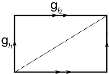
Figure 3: A torus represented by a rectangle with opposite sides identified. Each independent loop of the torus is assigned a group element $g_{l_{1}}$ and $g_{l_{2}}$ respectively.

We can represent it by a rectangle, with opposite edges identified. A simple triangulation would be to introduce an extra edge on the diagonal of the rectangle. Now any one edge of each of the triangles is a loop, since all the vertices of the rectangle are identified. According to (40), we therefore have $g_{aa}=1$ as the only possible configuration. However, from the point of view of the gauge theory, it is also possible to assign non-trivial values to the sides of the rectangle. Explicitly, considering one of the two triangles that make up the rectangle, and label the states of the two external edges by $g_{l_{1}},g_{l_{2}}$. The flatness condition requires only that the diagonal is restricted to take values equal to $g_{l_{1}}g_{l_{2}}$, and that for consistency between the two triangles sharing the same diagonal, $g_{l_{1}}$ and $g_{l_{2}}$ has to commute.

Recall that in the lattice gauge theories, $d$-cocycles $\alpha_{d}$ arise naturally in the fixed point wavefunction. These can be related to those $d$-cocycles $\nu_{d}$ defined in Ref. Chen et al., 2011a discussed above. The fact that $\nu_{d}$ is a function of $d+1$ group elements, and that it is invariant under the multiplication of all group elements by the same $g$ is precisely the statement that $g_{ab}$ is insensitive to this transformation, and $\alpha_{d}$ is invariant.

The $d$-cocycles $\alpha_{d}$ arising in the topological lattice gauge theories are identified with $\nu_{d}$, except that the input values of the function has to be translated according to Eqn. (40). Making the substitution into $\alpha_{d}$ reproduces the known relation between $\nu_{d}$ and a $d$ cocycle as described above in Eqn. (38). We recall that a $d$ cocycle is geometrically defined on the $T^{d}$ simplex, which is topologically equivalent to a $d$ ball, whose loops are contractible. Therefore the lattice gauge theory and the SPT phase agree there.

Finally we can compare the path-integral of the lattice gauge theory with Eqn. (39). For the SPT path integral, it is known that before taking the overall sum over states, the action itself is equal to one in all closed manifold. Therefore the path integral is simply equal to the total number of configurations, given by ${|G|^{N_{v}}}$, where $N_{v}$ is the total number of vertices. This can be interpreted roughly as the volume of the manifold. If a state contains long-range entanglement, a non-trivial constant term independent of volume should be expected, encoding information, for example about ground state degeneracies. Therefore the SPT phase is considered topologically trivial. Now, on a three manifold with $n_{0}$ disconnected components, but that all the loops are contractible, the field configurations between the theories are simply related by the $|G|^{n_{0}}$-to-1 map, and $Z_{\textrm{SPT}}$ is equal to $\mathcal{N}Z_{CS}$ up to volume independent choice of normalization factor $\mathcal{N}$. The situation, however is more non-trivial if we begin to consider manifolds with non-contractible loops. In those cases, the lattice gauge theories would then involve a sum also over Wilson lines. We will give some simple examples of these non-trivial factors in the example sections.

While we have been discussing a duality relation between SPT phases and lattice topological gauge theories (or Chern-Simons theories) in the case for finite discrete groups $G$, we note that SPT phases can still be defined for continuous $G$. In that case, $\nu_{d}$ are not simple smooth functions of the group variables, but instead are chosen to be Borel measurable functionsChen et al. (2011a). They are classified by Borel group cohomology ${\cal H}_{B}^{d}(G,\mathbb{R}/\mathbb{Z})$. As discussed earlier, while it is not immediately clear what the corresponding lattice gauge theories should be except when the connection is sufficiently close to vanishing, the Chern-Simons theories constructed from differential characters are classified by $H^{d+1}(BG,\mathbb{Z})\cong{\cal H}_{B}^{d}(G,\mathbb{R}/\mathbb{Z})$. Therefore the correspondence between Chern-Simons theories and SPT phases persists even for continuous $G$ in all space-time dimensions.

VI Duality Relations with String Net models

In Levin-Wen $2+1$ dimensional string-net models, each model is uniquely defined by a set of data: $\{\mathcal{F},F,N,\{d_{g}\}\}$, where $N$ is the number of string types in addition to the trivial state, $\mathcal{F}$ denotes the fusion rules of the string states when three meet at a vertex, and $F$ are the $6j$-symbols that control crossing relations between different orders of fusing three states $I,J,K$. (i.e. $(I\otimes J)\otimes K$ verses $I\otimes(J\otimes K)$.) Ultimately it also controls the form of the Hamiltonian. The quantum dimension $d_{I}$ is assigned to each string type.

Each state of the system is defined on a 2 dimensional (closed) surface. String states reside on edges of a trivalent lattice i.e. each vertex is connected to three edges. The most studied example is the honeycomb lattice, although in principle the lattice can be irregular. The string state is labeled by a representation of a group. In the case of Abelian groups, representation of the group is in 1-1 correspondence with group elements and thus interchangeable. In the case of non-Abelian groups it is also possible to perform the analogue of Fourier transformation to obtain a dual description in terms of group elementsBuerschaper and Aguado (2009). We will therefore for simplicity focus our discussion on Abelian groups such that there is no real distinction between group elements and irreducible representations up to a rescaling by phases of the basis states, and we can use the two basis interchangeably. A generalization to general groups would require following the procedure set out in Ref. Buerschaper and Aguado, 2009 carefully. In the following therefore, each edge of the string-net lattice is associated with a group element $g_{e}\in G$ for some Abelian group $G$. An orientation is also assigned to each edge, but the labeling is redundant– the same state can be described by the element $g_{e}^{-1}$ if the orientation is reversed. At each vertex only three strings meet. The fusion rule then dictates that the incoming string states that meet at a vertex product to identity.

To each configuration of the string-net, we associate to it a wavefunction $\Phi$. These wavefunctions satisfy a set of local rules, which are postulates motivated by the physical requirement that they describe states that are at fixed points of the renormalization group flow. These local rules can be summarized as follows:

$$\Phi\begin{pmatrix}\leavevmode\hbox to12.98pt{\vbox to15.83pt{\text{[drawing]}}}\leavevmode\hbox to18.97pt{\vbox to7.2pt{\text{[drawing]}}}\leavevmode\hbox to12.98pt{\vbox to15.83pt{\text{[drawing]}}}\end{pmatrix} i i =\Phi\begin{pmatrix}\leavevmode\hbox to12.98pt{\vbox to15.83pt{\text{[drawing]}}}\leavevmode\hbox to23.16pt{\vbox to7.77pt{\text{[drawing]}}}\leavevmode\hbox to12.98pt{\vbox to15.83pt{\text{[drawing]}}}\end{pmatrix} i i$$ (41a)

$$\Phi\begin{pmatrix}\leavevmode\hbox to12.98pt{\vbox to15.83pt{\text{[drawing]}}}&\leavevmode\hbox to11.78pt{\vbox to11.94pt{\text{[drawing]}}}\end{pmatrix} i i =d_{i}\Phi\begin{pmatrix}\leavevmode\hbox to12.98pt{\vbox to15.83pt{\text{[drawing]}}}\end{pmatrix}$$ (41b)

$$\Phi\left(\begin{matrix}\vspace{-3pt}\leavevmode\hbox to34.54pt{\vbox to14.06pt{\text{[drawing]}}}\end{matrix}\right) k l i j k l i j =\delta_{ij}\Phi\left(\begin{matrix}\vspace{-3pt}\leavevmode\hbox to34.54pt{\vbox to14.06pt{\text{[drawing]}}}\end{matrix}\right) k l i i k l i i$$ (41c)

$$\Phi\left(\begin{matrix}\vspace{-3pt}\leavevmode\hbox to32.84pt{\vbox to28.33pt{\text{[drawing]}}}\end{matrix}\right) j_{\text{\scalebox{0.7}{$1$}}} j_{\text{\scalebox{0.7}{$2$}}} j_{\text{\scalebox{0.7}{$3$}}} j_{\text{\scalebox{0.7}{$4$}}} m j_{\text{\scalebox{0.7}{$1$}}} j_{\text{\scalebox{0.7}{$2$}}} j_{\text{\scalebox{0.7}{$3$}}} j_{\text{\scalebox{0.7}{$4$}}} m =\sum\limits_{n}F^{j_{1}j_{2}m}_{j_{3}j_{4}n}\Phi\left(\begin{matrix}\vspace{-3pt}\leavevmode\hbox to31.21pt{\vbox to29.42pt{\text{[drawing]}}}\end{matrix}\right), j_{\text{\scalebox{0.7}{$1$}}} j_{\text{\scalebox{0.7}{$2$}}} j_{\text{\scalebox{0.7}{$3$}}} j_{\text{\scalebox{0.7}{$4$}}} n j_{\text{\scalebox{0.7}{$1$}}} j_{\text{\scalebox{0.7}{$2$}}} j_{\text{\scalebox{0.7}{$3$}}} j_{\text{\scalebox{0.7}{$4$}}} n$$ (41d)

The duality relation with the topological lattice gauge theory is closely related to the duality relation already discussed in Levin and Gu (2012) between the string-net model and the SPT phase. We note however that for the three dimensional topological lattice gauge theory, the triangulation is taken over the entire 3$d$ space-time manifold. The string-net state we have described above, however, is understood as a state at a particular time in Hamiltonian formulation. Therefore, it is not hard to guess that the wavefunction $\Phi$ is related to the topological lattice gauge theory path integral with a boundary. The relation between wavefunction and path-integral is well known in the context of (conformal) quantum field theories. The wavefunction is, up to normalization, understood as a path integral that integrates over all the paths connecting a state from $t=-\infty$ to some state at finite $t_{0}$. A state at a given time-slice really means boundary conditions on the fields. In the lattice gauge theory path-integral, the gauge fields $g_{ij}$ also satisfy fixed boundary conditions respected by the path integral. A given configuration of these boundary degrees of freedom denoted by $\Gamma_{\textrm{dual}}$ can be mapped to a unique string-net state $\Gamma$. To make the map precise, the 2-dimensional fixed time slice inherits a triangulation from the triangulation of the entire 3-manifold, and a group element is again attached to each edge of the triangles. This triangular lattice is a dual lattice of the honeycomb lattice. i.e. The triangular lattice is given by the set of vertices that reside at the center of each hexagon of a given honeycomb lattice, as shown in Fig. 4.

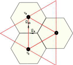
Figure 4: String net on a honeycomb lattice and the dual triangular lattice on which the lattice gauge theory is defined.

Each edge on the honeycomb lattice therefore cuts through precisely one edge on the triangular lattice that connects two nearest neighbor vertices. This suggests that one should identify the string state $g_{e}$ on an edge $e$ and the gauge state on the edge of the triangular lattice $g_{ab}$ intersecting $e$. The orientation of the string state $g_{e}$ in the duality can be chosen by convention, as depicted in Fig. 4. Ultimately the duality is such that a face is mapped to a vertex and vice versa, whereas an edge is mapped back to an edge. The honeycomb lattice serves only as an example to illustrate the relation, but the relation survives independently of the precise choice of the lattice, as long as it is trivalent. This is necessary since the local rules described in Eq. (41-41d) do not generally preserve the lattice structure.

The explicit relation between the string-net wavefunction $\Phi(M_{2},\Gamma)$ on a closed 2d surface $M_{2}$ for a given string-net configuration $\Gamma$, and the path integral $Z_{CS}(B,\Gamma_{\textrm{dual}})$ of the topological lattice gauge theory on a 3d manifold $B_{3}$ where $\partial B_{3}=M_{2}$ with corresponding boundary gauge configurations $\Gamma_{\textrm{dual}}$, is then given by

$$\ \ \ \Phi(M_{2})[\Gamma]=\frac{\mathcal{N}[\Gamma]}{|G|^{N_{v_{\textrm{int}}}}}Z_{CS}(B_{3})$$ (42)

$$=\frac{\mathcal{N}[\Gamma]}{|G|^{N_{v_{\textrm{int}}}}}\sum_{\{g_{ab}\}_{a,b\in\{v_{\textrm{int}}\}}}\prod_{i}\alpha^{s_{i}}(\{g_{cd}\},\{v_{c,d}\in T_{i}\}),$$

where $\{v_{\textrm{int}}\}$ denotes the set of vertices lying in the interior of $B_{3}$, and $N_{v_{\textrm{int}}}$ is the total number of these internal vertices, and $\mathcal{N}[\Gamma]$ is some normalization that depends on the specific string-net configuration, or surface gauge configuration, denoted by $\Gamma$. This corresponds to the freedom in the string-net model to choose a basis set of wavefunctions for each configuration. The wavefunctions are however chosen to be related to each other by specific rules Ref. Levin and Gu, 2012, which has specific meanings in the lattice gauge theory as we will explain below. Using the duality relations, we note immediately that $\alpha(\{g_{ab}\})$, the action defined on a single tetrahedron, is proportional to the string-net wavefunction also on a tetrahedron. Given the cocycle condition satisfied by $\alpha(\{g_{ab}\})$, the wavefunction is clearly independent of the precise triangulation in the interior of the manifold $B_{3}$.

In the normalization chosen in Ref. Levin and Gu, 2012, the wavefunction of a string-net on the tetrahedron as depicted in Fig. 5 is given by

$$\Phi(T)=v_{g_{i}}v_{g_{j}}v_{g_{k}}v_{g_{l}}F^{g_{i}g_{j}g_{m}}_{g_{k}g_{l}g_{n}},$$ (43)

where $F^{g_{i}g_{j}g_{m}}_{g_{k}g_{l}g_{n}}$ is a component of the $6j$-symbol, and $v_{g_{i}}^{2}\equiv d_{g_{i}}=\pm 1$ for Abelian groups. The six elements involved are not independent due to fusion rules. In fact

$$g_{m}=g_{k}g_{l}\,,\qquad g_{n}=g_{k}g_{j}\,,\qquad g_{i}g_{j}g_{k}g_{l}=1.$$ (44)

The $6j$ symbols satisfy the pentagon relations, and that the pentagon relations are invariant under a rescaling of $F$’s, corresponding to a rescaling of each of the vertices. i.e.

$$F^{g_{i}g_{j}g_{m}}_{g_{k}g_{l}g_{n}}\to\frac{f(g_{i},g_{l},g_{n})f(g_{j},g_{k},g_{n}^{-1})}{f(g_{i},g_{j},g_{m})f(g_{k},g_{l},g_{m}^{-1})}F^{g_{i}f_{j}g_{m}}_{g_{k}g_{l}g_{n}}.$$ (45)

where the phase factor $f(g_{i},g_{l},g_{n})$ is symmetric under cyclic rotation of the three elements, and recall that of which only two are independent since the fusion constraint requires that $g_{i}g_{l}g_{n}=1$. We therefore identify the set of $6j$ symbol as a 3-cocycle in $H^{3}(G,U(1))$ in group cohomology, and that the above rescaling is a rescaling of a 3-cocycle by a coboundary $\delta\beta$ for some 2-cochain $\beta$. i.e.

$$\beta(g_{i},g_{l})=f(g_{i},g_{l},g_{n}).$$ (46)

Carefully comparing the transformation property of $\alpha(g_{ab},g_{bc},g_{cd}),\,a<b<c<d$ under rescaling by a co-boundary we therefore have

$$v_{g_{i}}v_{g_{j}}v_{g_{k}}v_{g_{l}}F^{g_{i}f_{j}g_{m}}_{g_{k}g_{l}g_{n}}=\mathcal{N}[\{\Gamma_{\textrm{tetrahedron}}\}]\alpha(g_{i},g_{j},g_{k}),$$ (47)

and therefore

$$\mathcal{N}[\Gamma_{\textrm{tetrahedron}}]=v_{g_{i}}v_{g_{j}}v_{g_{k}}v_{g_{l}}.$$ (48)

Figure 5: The string net dual of a tetrahedron which is still a tetrahedron.

There is however one important distinction between the string-net model and the topological lattice gauge theory. That is, the string-net wavefunction defined on a tetrahedron is chosen such that it respects the tetrahedron symmetry, and that the branching structure introduced in the lattice gauge theory is absent. This imposes very severe constraint on the solution of the $6j$-symbols, and as a result, the solutions considered in such highly symmetric string-net models do not span the full $H^{3}(G,U(1))$, where this is also observed for example for the explicit case of $G=\mathbb{Z}_{3}$ in Ref. Hung Wen, 2012. Generalization via introducing a branching structure is clearly possible, particularly given the duality relation with the lattice gauge theory. Numbered vertices on the surface of the lattice gauge theory is dual to plaquettes of the string-net lattice. The branching structure therefore admits a direct translation.

As mentioned above, the wavefunction $\Phi$ of a string-net configuration can be related to some other configurations via a set of local rules. These local rules have simple implementation from the the perspective of the path integral of the topological lattice theory.

VI.1 Crossing relation

Eq. (41d) is referred to as the crossing relation which has a dual in the lattice gauge theory as relating two sets of triangles, depicted as in Fig. 6. The crossing transformation on the wavefunction corresponds to placing an extra tetrahedron $T$ right on top of the specific triangles. i.e. two of the triangular surfaces of $T$ is matched/glued to the two surface triangles involved. Since there isn’t any extra internal vertices involved, this addition lead only to an extra factor $\alpha(\{g_{ab}\})$ in the path integral, exactly as expected of the transformation property of the string-net wavefunction $\Phi$.

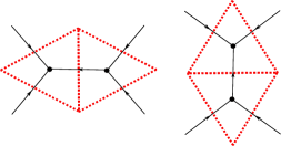
Figure 6: Crossing relations in the dual lattice gauge theory (in dotted red lines).

VI.2 Removal of isolated loops

In the string-net model, an isolated loop of string type $i$ can be removed as the wavefunction acquires an extra factor of $d_{i}$, the quantum dimension of the string type $i$. Consider a small loop in the string-net model. It corresponds to three triangles meeting such that together they form a larger triangle, as shown in Fig. 7.

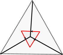
Figure 7: A loop in the string-net model, and its dual in the lattice gauge theory. .

The gauge configuration is such that the internal lines take values $i$, and the external edges of the large triangle are in the trivial state. Topologically, that is precisely a tetrahedron fitted at the surface. Since all the edges belong to the boundary, there is no summation required over the states on the tetrahedron, and this is a simple factor. Therefore, we could replace the tetrahedron by its numerical value. At the same time, an extra phase factor factor is attached accounting for the removal of the three edges. This factor is chosen to be $d_{i}$, which we recall is $\pm 1$ for Abelian groups. We note that any loop can be reduced via multiple crossings to the basic loop involving the three triangles described above.

We note that these rules uniquely determine the ground state wavefunction. However, the wavefunction itself is not a topological object. If we were to compute ground state degeneracy of the string-net on a closed 2d manifold $\Sigma_{g}$ of genus $g$, it is given by the following:

$$\textrm{degeneracy}(\Sigma_{g})=\sum_{i}\Phi[V_{i}]\Phi^{*}[V^{i}],$$ (49)

where $V_{i}$ denotes the basis for ground states. We recognize the above, given the relationship Eq. (42), as gluing two path integrals, each of which defined on 3-manifolds $\Sigma_{g}\times I$, for some finite interval $I$, along the common boundary $\Sigma_{g}$. Since the normalization factor $\mathcal{N}[\Gamma]$ is a phase, it is canceled out in the computation of degeneracy, and we are left with a path integral of the topological lattice theory over a closed 3-manifold $\Sigma_{g}\times S^{1}$, which is a topological invariant.

VII Some simple examples

In this section, we would like to give some simple examples of these lattice gauge theories. We would particularly be interested in finite gauge groups $G$ in one and two spatial dimensions.

VII.1 $d$=3

To begin with we will take the above construction and study the explicit form of the action of the lattice topological gauge theory for a finite group $G$ at $d=3$, the case which has already been discussed in detail in Ref. Dijkgraaf and Witten, 1990.

Recall that a triangulation of a three manifold $M_{3}$ is given by

$$M_{3}=\sum_{i}\epsilon_{i}T_{i},$$ (50)

where $T_{i}$ are 3 simplices, or in other words tetrahedra. There are 4 vertices and 6 edges on a tetrahedron. As already discussed in the previous section, each edge connecting vertices $v_{i}$ and $v_{j}$ is assigned a group element $g_{ij}$. To make the assignment unambiguous, one needs to give an orientation to each edge, and thus a branching structure to the tetrahedron. This is achieved by numbering the vertices, from 0 to 3. Of the 6 group elements assigned to the 6 edges, only three of them are independent. To see that, we recall that each 2-simplex, or triangle, lead to one constraint between the edges. However, these constraints are not independent. For a tetrahedron, the fact that the triangles together form a closed surface (ie the boundary of the tetrahedron) signals that there is one redundant constraint. Therefore the number of independent degrees of freedom is given by

dof $$= \textrm{\# edges}-(\textrm{\# triangles}-\textrm{\# connected piece})$$ (51)

$$= C^{4}_{2}-C^{4}_{3}+C^{4}_{4}=3,$$

$C^{d}_{i}$ are binomial coefficients.

Let us note that this result can be generalized easily to general dimensions.

$$\textrm{dof}_{d-\textrm{simplex}}=\sum_{i=2}^{d}(-1)^{i}C^{d}_{i}=d.$$ (52)

VII.1.1 Path-integrals for $\mathbb{Z}_{N}$

To compute the path-integral of the lattice gauge theory on a general three manifold, it is useful to first consider the special case where the manifold concerned is given by $Y\times S^{1}$, where $Y$ is a 2-sphere with three holes. The triangulation is represented in Fig. 8, where the sphere is represented by the triangle whose three vertices are identified, and the holes by the three edges, and $S^{1}$ corresponds to the vertical edge perpendicular to the triangle.

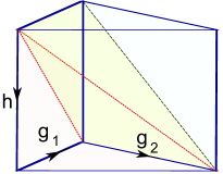
Figure 8: The cellurarization into three tetrahedrons of $Y\times S^{1}$.

Strictly speaking, this is not a triangulation but a cellularization since each edge connects to the same vertex. The naive branching structure obtained by ordering the vertices become ill-defined, since there is only one vertex. A rigorous triangulation would require adding extra vertices to our present construction. However that does not affect the final result of the path-integral given its nature as a topological invariant. For simplicity as in Ref. Dijkgraaf and Witten, 1990, we keep to this simple cellularization, but replace the branching structure by explicitly specifying the orientation of each edge. A group element is assigned to each of the cycles, subjected to the flatness condition on the triangle. The consistency condition also immediately follows:

$$[h,g_{i}]=1.$$ (53)

Again, the above condition is a result of considering the group element assignment to diagonals on any of the vertical rectangles. Since the manifold is open, no summation is required over the group elements, and the path-integral with the orientation assignment as in the figure is given by

$$Z_{Y\times S_{1}}=\frac{1}{|G|}\frac{\alpha(h,g_{1},g_{2})\alpha(g_{1},g_{2},h)}{\alpha(g_{1},h,g_{2})}\equiv\frac{1}{|G|}c_{h}(g_{1},g_{2}).$$ (54)

It is denoted $c_{h}(g_{1},g_{2})$ because it can be readily shown that it is a 2-cocycle of the group $N_{h}$, where $N_{h}\subset G$ denotes the subgroup whose elements commute with $h$. From the relation between $c_{h}(g_{1},g_{2})$ and the 3-cocycles $\alpha$, we should rewrite $|G|Z_{Y\times S_{1}}=c_{h}^{\epsilon}(g_{1},g_{2})$. If the orientation of the triangle aligns with that of the vertical edge we obtain $\epsilon=+1$, and $\epsilon={\dagger}$ otherwise.

Path-integrals of more general three manifolds can be obtained by gluing together $Z_{Y\times S_{1}}$ via the gluing conditions Eq. (36).

One important class of three manifolds are of the form $\Sigma_{g}\times S^{1}$, where $\Sigma_{g}$ is a genus $g$ two dimensional closed surface. The path-integral evaluated on these manifolds can be interpreted as ground state degeneracy of the system residing in the spatial slice $\Sigma_{g}$. The cellularization of a $\Sigma_{g}\times S^{1}$ is demonstrated in Fig. 9.

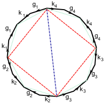
Figure 9: A depiction of the genus four surface $\Sigma_{4}$. The extra circle $S^{1}$ described in the text is suppressed. Edges assigned the same group element is also identified. The dashed lines correspond to our canonical choice of dividing the three dimensional block into $Y\times S^{1}$, which is then used for the computation of the partition function.

It is readily built up from a collection of $Y\times S^{1}$. A group element is assigned to each non-trivial loop, and we therefore have the collection $\{g_{i},k_{i}\},\,\,1\leq i\leq g$. For consistency we again require that

$$\prod^{g}_{i}[g_{i},k_{i}]=1\,,\qquad[h,g_{i}]=[h,k_{i}]=1,$$ (55)

where $1\leq i\leq g$. The path-integral is then given by a sum over all $h,g_{i},k_{i}$ subjected to the above constraints,

$$Z_{\Sigma_{g}\times S^{1}}=\frac{1}{|G|}\sum_{g_{i},k_{i},h}\prod_{i_{1}}^{g}\frac{c_{h}(g_{i_{1}},k_{i_{1}})}{c_{h}(k_{i_{1}},g_{i_{1}})}$$

$$\prod_{i_{2}}^{g}c_{h}(g_{i_{2}}k_{i_{2}},(k_{i_{2}}g_{i_{2}})^{-1})\prod_{i_{3}}^{g-3}c_{h}(\prod_{j}^{i_{3}}x_{j},x_{i_{3}+1})$$ (56)

where $x_{i}=[g_{i},k_{i}]$. To understand the above form, we note that the first product corresponds to the outermost set of triangles bounded by the boundary of the polygon and the light blue lines in Fig. 9; the second product corresponds to the set of triangles bounded between the light blue lines and the red lines. Cutting along the light blue and red lines give several blocks of $Y\times S^{1}$, which contribute to the first two products. Then we are always left with a $g$-gon for a genus $g$ surface. The third set of products then correspond to triangulating the remaining $g$-gon by connecting a chosen vertex with all other vertices except its own nearest neighbor. There are thus $g-3$ such vertices. In Fig. 9 there is exactly $4-3=1$ such cut corresponding to the deep blue line.

Consider specifically $\mathbb{Z}_{N}$ groups. The 3-cocycles of $\mathbb{Z}_{N}$ is given by Moore and Seiberg (1989)

$$\alpha_{k}(g_{1},g_{2},g_{3})=\exp(\frac{2\pi ik\bar{g}_{1}}{N^{2}}(\bar{g}_{2}+\bar{g}_{3}-\overline{(g_{2}+g_{3})})),$$ (57)

for some appropriate $k\in\mathbb{Z}$, and $g_{i}\in\mathbb{Z}_{N}$, and $\bar{x}=x\,\,\,\textrm{mod}N$ for $x\in\mathbb{Z}$. There are altogether $N$ distinct choices of $k$ that give rise to representatives of the $N$ different group cohomology classes in $H^{3}(\mathbb{Z}_{N},U(1))$. However, substituting the above expression into Eq. (56) the summands become identically 1, independently of $k$! Taking also into account that the group is Abelian and thus the constraints in Eq. (55) are trivially satisfied, the sum simply separately counts the possible Wilson loop around each of the $2g$ cycles in $\Sigma_{g}$. Therefore, we have

$$Z_{\Sigma_{g}\times S^{1},G=\mathbb{Z}_{N}}=N^{2g}.$$ (58)

This is a special case of the result obtained in Ref. Dijkgraaf and Witten, 1990 for more general finite groups $G$. We note that at the end this appears to have no dependence on the 3-cocycle $\alpha$ we have chosen. The reason is that these manifolds $\Sigma_{g}\times S^{1}$ can all be computed by cutting them into blocks of $Y\times S^{1}$. As we have seen in Eq. (54) the 3-cocycles always come in combinations to form $c_{h}(g_{1},g_{2})$. These are classified by $H^{2}(N_{h},U(1))$. For Abelian groups these are trivial, and for more general groups, they are in general different from $H^{3}(\mathbb{Z}_{N},U(1))$. Since our path-integral on $\Sigma_{g}\times S^{1}$ is equal to the ground state degeneracy, it is perhaps not surprising that the ground state degeneracy alone does not distinguish all topological phases.

VII.1.2 The $S$ and $T$ matrix

There are two other important quantities required to obtain the partition function on general 3-Manifolds. These are the so called $S$ and $T$ matrices which describe how the partition function on a 3-manifold $M$ whose boundary is a torus transforms under modular transformation of the torus. So far we have been working with a basis for the Hilbert space given by different configurations of group elements assigned on the edges residing on the boundary of $M$. To make closer connections with Chern-Simons theory, it is useful to make a change of basis and label the states in terms of representations. Note that this change of basis is exactly the same transformation that connects the lattice gauge theory and the string-net models discussed in the previous section. In such a basis, through the relationship of the lattice gauge theory with 2-dimensional orbifold theories, the $S$ matrix is known to beDijkgraaf et al. (1989)

$$S^{AB}_{\alpha\beta}=\frac{1}{|G|}\sum_{h\in C_{B},g\in C_{A},[h,g]=1}\rho^{g}_{\alpha}(h^{-1})\rho^{h}_{\beta}(g^{-1})\sigma(g|h),$$ (59)

where $C^{A,B}$ denote conjugacy classes of the group $G$ and $\rho^{g}_{\alpha}=\textrm{tr}R^{g}_{\alpha}$, where $R^{g}_{\alpha}$ is a representation of the stabilizer group $N_{g\in C^{A}}$ containing elements that commute with $g$. The subscript $\alpha$ enumerates these representations for each $N_{g\in C^{A}}$. Since $N_{g}$ is isomorphic to each other for all $g$ belonging to the same conjugacy class, $N_{g}$ is equivalently denoted as $N_{A}$. Correspondingly, the $T$ matrix is given by

$$T^{AB}_{\alpha\beta}=\delta_{\alpha\beta}\delta^{AB}\rho^{g}_{\alpha}(g)\rho^{g}_{\alpha}(1)^{-1}\sigma(g|g)^{-1/2}.$$ (60)

For Abelian groups, $H^{2}(G,U(1))$ is trivial. The phase $\sigma(g|h)$ treated as a 1-cochain in $N_{h}$ is then related to $c_{h}(g_{1},g_{2})$ by

$$c_{h}(g_{1},g_{2})=\frac{\sigma(g|h_{1})\sigma(g|h_{2})}{\sigma(g|h_{1}h_{2})}.$$ (61)

Consider $\mathbb{Z}_{N}$. In this case there are $N$ distinct classes in $H^{3}(\mathbb{Z}_{2},U(1))$, with representative as already given in Eq. (57). Using Eq. (54, 61), we can read off $\sigma(g|h)$. They are given by

$$\sigma_{(k)}(g|h)=\exp(\frac{2\,i\pi kgh}{N^{2}}).$$ (62)

Also all stabilizer subgroups $N_{A}=\mathbb{Z}_{N}$. For concreteness, let us consider $N=2$. In which case $k=0$ or $k=2$. As a result $\rho^{g}_{\alpha}(h)=(-1)^{\alpha h}$, where both $\alpha$ and $h$ can take values $\pm 1$. Substituting into Eq.(59, 60), and writing them as $4\times 4$ matrices, we have the following two sets of $S,T$ matrices:

$$T(k=0) =\textrm{diag}(1,1,1,-1),$$ (63)

$$S(k=0) =\frac{1}{2}\left(\begin{array}[]{cccc}1&1&1&1\\ 1&1&-1&-1\\ 1&-1&1&-1\\ 1&-1&-1&1\end{array}\right),$$ (68)

and

$$T(k=2) =\textrm{diag}(1,i,-i,1),$$ (69)

$$S(k=2) =\frac{1}{2}\left(\begin{array}[]{cccc}1&1&1&1\\ 1&-1&1&-1\\ 1&1&-1&-1\\ 1&-1&-1&1\end{array}\right).$$ (74)

These matrices are precisely those $S$ and $T$ matrices obtained in Ref. Levin and Wen, 2005 for the two distinct $\mathbb{Z}_{2}$ string-net models. As discussed there, these $S$ and $T$ matrices also arise from $U(1)\times U(1)$ Chern-Simons theories. The $k=0$ $\mathbb{Z}_{2}$ lattice gauge theory is equivalent to the $U(1)\times U(1)$ Chern-Simons theory with $K$-matrix

$$K_{0}=\left(\begin{array}[]{cc}0&2\\ 2&0\end{array}\right),$$ (75)

whereas the $k=2$ theory corresponds to

$$K_{2}=\left(\begin{array}[]{cc}2&0\\ 0&-2\end{array}\right).$$ (76)

Ironically, the correspondence underlies the fact that a gauge group in a gauge theory is not really a physical object, but rather a tool in constructing redundancy in a theory.

VII.2 $d$=2

Having discussed the case of $d=3$, let us also look at some simple examples in $d=2$. Our discussion in this paper so far has refrained from including $d=2$. The reason is that in 2 dimensions it is well known that long range order is necessarily destroyed by strong quantum fluctuations. In 2$d$ gapped systems without symmetries, which is the case of a weakly coupled gauge theory necessarily belong to the same phaseChen et al. (2011a). We believe the phases studied here is ultimately unstable. More specifically, the flatness condition crucial to these phases probably does not survive quantum fluctuations. We study examples in one spatial dimensions to illustrate some features of these lattice gauge theories and their corresponding partition function, in the hope that some of the characteristics of the action can be extrapolated in higher dimensions.

In this case a triangulation of a two manifold $M_{2}=\sum_{i}\epsilon_{i}T_{i}$ divides the manifold into triangles $T_{i}$. Each triangle would then be associated with a 2-cocycle $\alpha_{2}\in H^{2}(G,U(1))$. For a general closed orientable genus $g$ manifold $\Sigma_{g}$, we can adopt basically a very similar cellularization as in the $d=3$ case where $M_{3}=\Sigma_{g}\times S^{1}$, and the final result of the path-integral is simply given by the same expression (61), except that each $c_{h}(g_{i},k_{i})$ is replaced by $\alpha_{2}(g_{i},k_{i})$, and that there is one less summation over Wilson loops along the extra $S^{1}$ there. For Abelian groups, $H^{2}(G,U(1))=0$, and we can simply take $\alpha_{2}(g,k)\equiv 1$. Therefore, the result is simply given by

$$Z_{\Sigma_{g}}=|G|^{2g-1}.$$ (77)

We would like to pause here and comment on the case where $G$ contains time-reversal $\mathbb{Z}^{T}_{2}$. In this case, all group elements are divided into two groups, such that each element $g\in G$ is assigned a value $t(g)=\pm 1$. The $n$-cocycle condition is modified to

$$(d_{n}\alpha_{n})(g_{1},\cdots,g_{n+1})=$$

$$\alpha_{n}^{t(g_{1})}(g_{2},\cdots,g_{n+1})\alpha_{n}^{(-1)^{n+1}}(g_{1},\cdots,g_{n})$$

$$\prod_{i}^{n}\alpha_{n}^{(-1)^{i}}(g_{1},\cdots,g_{i-1},g_{i}f_{i+1},g_{i+2},\cdots g_{n+1}).$$ (78)

SPT phases with time-reversal symmetry has been discussed already in Ref. Chen et al., 2010. Here, following completely analogous construction of the lattice gauge theory, we can define a path-integral for a lattice gauge theory which gauges time reversal symmetry! The path-integral is given by

$$Z_{M}({G\supset\mathbb{Z}^{T}_{2}})=$$

$$|G|^{-N_{v}}\sum_{\{g_{ab}\}}\prod_{i}\alpha^{s_{i}*t(g_{b})}(\{g_{cd}\},\{v_{c,d}\in T_{i}\}).$$ (79)

Here $s_{i}$ depends on the orientation of the $d$-simplex $T_{i}$ as explained in section II. The new ingredient is $t(g_{p_{i}})$. Recall that we have assigned a branching structure to the triangulation, giving an order to the vertices, both locally on each simplex, and globally. This defines a special base point $P_{0}$ in the space-time manifold, i.e. the vertex with the smallest index, and also a base point $p_{i}$ in each simplex. Consider a path connecting $P_{0}$ and $p_{i}$, passing through vertices $v_{1},v_{2},\cdots v_{n}$, then we define $g_{p_{i}}=g_{P_{0}v_{1}}g_{v_{1}v_{2}}\cdots g_{v_{n}v_{p_{i}}}$. The value $t(g_{p_{i}})$ is then $+1$ or ${\dagger}$ depending on $g_{p_{i}}$. Note that $t(g_{1}g_{2})=t(g_{1})t(g_{2})$, therefore the assignment of $t(g_{p_{i}})$ to each simplex is independent of the path chosen to connect the base points. Homotopic paths would automatically give the same $t(g_{p_{i}})$.

We would like to compute the path-integral for the simplest case where $G=\mathbb{Z}_{2}^{T}$ for $d=2$. In this case, $H^{2}(\mathbb{Z}_{2}^{T},U(1))=\mathbb{Z}_{2}$. The explicit form of representative cocycle from each class of $H^{2}(\mathbb{Z}_{2}^{T},U(1))=\mathbb{Z}_{2}$ has been computed in Ref. Chen et al., 2010. We represent $\mathbb{Z}_{2}^{T}=\{0,1\}$, and we take the only non-trivial consistent choice of $t(0)=1$, and $t(1)={\dagger}$. Group multiplication is then taken as addition of group elements modulo 2. By making use of rescalings using coboundaries, it is demonstratedChen et al. (2010) that it is convenient to exhaust the redundancy by rescaling all components to 1, leaving behind only $\alpha(1,1)$. A representative of each of the classes is then given by $\alpha(1,1)=\pm 1$. Therefore, we can rewrite the two classes as

$$\alpha_{\pm}(g_{1},g_{2})=\exp(\frac{i\pi(1\mp 1)}{2}g_{1}g_{2}).$$ (80)

The fact that these 2-cocycles can be made completely real actually tells us that the extra group action $t(g_{p_{i}})$ attached to each $\alpha$ on each simplex does not lead to anything new in this particular case. Substituting these $\alpha$ into the path-integral Eq.(79) should yield the same answer as $\mathbb{Z}_{2}$ for arbitrary closed orientable surface of genus $g$. Indeed, by explicit substitution, and the fact that $\sum_{i}^{g}(g_{i}+k_{i})=0$, we recover the result in Eq. (77) with $|G|=2$.

VIII Summary

In this paper, we consider weakly coupled lattice gauge theories where the charged particles have a large mass gap and the field strength fluctuations are weak at the lattice scale. A weakly coupled lattice gauge theory is described by the following imaginary-time path integral:

$$Z=\sum_{\gamma}e^{\hskip 1.0pt\mathrm{i}\hskip 1.0ptS_{\text{top}}[\{G_{ij}\}]-S_{\text{dyn}}[\{G_{ij}\}]}.$$ (81)

where $S_{\text{top}}[\{G_{ij}\}]$ is a topological term which is invariant under the coarse graining of lattice and is independent of “space-time metrics”. The dynamical term $S_{\text{dyn}}[\{G_{ij}\}]$ imposes the conditions of the large mass gap for the charged particles and the weak fluctuations for the field strength. We find that the quantized topological terms can be constructed systematically from the elements of topological cohomology classes $H^{d+1}(BG,\mathbb{Z})$ for the classifying space of the gauge group $G$ in $d$ space-time dimensions. This result is valid for any compact gauge groups (continuous or discrete) and in any dimensions. This generalizes the Chern-Simons topological terms and other form of topological terms previously known in gauge theory.

Our motivation to study quantized topological terms is to gain some general understanding of quantum phases of gauge theory. Since quantized topological terms cannot be modified under the renormalization flow, it is possible that adding a quantized topological term will cause the system to go to another phase. In $3$ space-time dimensions, the quantized topological terms correspond to generalized Chern-Simons terms, and adding a quantized topological term will always cause the system to go to another gapped phase. So the gapped phases of a weakly coupled lattice gauge theory is classified by quantized topological terms $H^{4}(BG,\mathbb{Z})$ in $3$ space-time dimensions.

For finite gauge groups, the weakly coupled lattice gauge theories are also in gapped phases which have non-trivial topological orders. In this case, can generalized Chern-Simons terms (ie $H^{d+1}(BG,\mathbb{Z})$) also classify the topological phases of weakly coupled lattice gauge theories?

For finite gauge groups, we may choose $S_{\text{dyn}}[\{G_{ij}\}]=\infty$ for gauge configurations with non-zero field strength, and $S_{\text{dyn}}[\{G_{ij}\}]=0$ for gauge configurations with zero field strength. In this case, the path integral eqn. (81) becomes topological (ie invariant under any coarse graining of the lattice.) Such lattice topological gauge theories are classified by $H^{d+1}(BG,\mathbb{Z})$ in $d$ space-time dimensions.

The lattice topological gauge theories do describe gapped phases of weakly coupled lattice gauge theories of finite gauge group. But do those gapped phases belong to different phases or not? Can those different gapped phases be smoothly connected by deforming $S_{\text{dyn}}[\{G_{ij}\}]$? Since the weakly coupled lattice gauge theories have no global symmetries, their gapped phases all belong to the same one phase in $2$ space-time dimensions.Verstraete et al. (2005); Chen et al. (2011c) So despite that $H^{3}(BG,\mathbb{Z})$ is non-trivial which leads to different lattice topological gauge theories, they all describe the same phase. However, in higher dimensions, there are non-trivial gapped phases for weakly coupled lattice gauge theories, and those gapped phases can be described by the quantized topological terms $H^{d+1}(BG,\mathbb{Z})$ in $d$ space-time dimensions. We have examples that different quantized topological terms do give rise to topological orders, as one can see from the calculation of the $S,T$ matrices.Wen (1990) However, it is not clear if the correspondence is one-to-one for a fixed gauge group in general.

This research is supported by NSF Grant No. DMR-1005541 and NSFC 11074140. Research at Perimeter Institute is supported by the Government of Canada through Industry Canada and by the Province of Ontario through the Ministry of Research. LYH is supported by the Croucher Fellowship.

Appendix A Relation between $H^{*}(BG,\mathbb{Z})$ and $H^{*}(BG,\mathbb{R}/\mathbb{Z})$

Since

$$0\to\mathbb{Z}\to\mathbb{R}\to U(1)\to 0,$$ (82)

we have

$$...\to H^{0}(BG,\mathbb{Z})\to H^{0}(BG,\mathbb{R})\to H^{0}(BG,\mathbb{R}/\mathbb{Z})\to$$

$$H^{1}(BG,\mathbb{Z})\to H^{1}(BG,\mathbb{R})\to H^{1}(BG,\mathbb{R}/\mathbb{Z})\to$$

$$\ \ \ \ \ \ \ \ \ \ \ \ \ \ \ \ \ \ ...\ \ ...$$ (83)

$$\to H^{d}(BG,\mathbb{Z})\to H^{d}(BG,\mathbb{R})\to H^{d}(BG,\mathbb{R}/\mathbb{Z})\to...$$

For a finite group $H^{d}(BG,\mathbb{R})=0$. This allows us to obtain

$$H^{d}(BG,\mathbb{R}/\mathbb{Z})\simeq H^{d+1}(BG,\mathbb{Z})\simeq{\cal H}_{B}^{d}(G,\mathbb{R}/\mathbb{Z}).$$ (84)

For a compact Lie group, $H^{d=\text{odd}}(BG,\mathbb{R})=0$. So we have, for $d=$ even,

$$0 \to H^{d-1}(BG,\mathbb{R}/\mathbb{Z})\to H^{d}(BG,\mathbb{Z})\to H^{d}(BG,\mathbb{R})$$

$$\to H^{d}(BG,\mathbb{R}/\mathbb{Z})\to H^{d+1}(BG,\mathbb{Z})\to 0$$ (85)

$0\to H^{d-1}(BG,\mathbb{R}/\mathbb{Z})\to H^{d}(BG,\mathbb{Z})$ means that each element in $H^{d-1}(BG,\mathbb{R}/\mathbb{Z})$ corresponds to a distinct element in $H^{d}(BG,\mathbb{Z})$. $H^{d}(BG,\mathbb{R}/\mathbb{Z})\to H^{d+1}(BG,\mathbb{Z})\to 0$ means that each element in $H^{d+1}(BG,\mathbb{Z})$ correspond to a set of elements in $H^{d}(BG,\mathbb{R}/\mathbb{Z})$. So we have, for $d=$ even,

$$H^{d-1}(BG,\mathbb{R}/\mathbb{Z}) \subset H^{d}(BG,\mathbb{Z})={\cal H}^{d-1}_{B}(G,\mathbb{R}/\mathbb{Z}),$$

$$H^{d}(BG,\mathbb{R}/\mathbb{Z})/\Gamma =H^{d+1}(BG,\mathbb{Z})={\cal H}^{d}_{B}(G,\mathbb{R}/\mathbb{Z}).$$ (86)

where the 0 element in $H^{d+1}(BG,\mathbb{Z})$ correspond to the subgroup $\Gamma\subset H^{d}(BG,\mathbb{R}/\mathbb{Z})$.

Appendix B Calculate $H^{d}(BG,\mathbb{R}/\mathbb{Z})$

We can use the Künneth formula (see Ref. Spanier, 1966 page 247)

$$\ \ \ \ H^{d}(X\times X^{\prime},M\otimes_{R}M^{\prime})$$

$$\simeq\Big{[}\oplus_{p=0}^{d}H^{p}(X,M)\otimes_{R}H^{d-p}(X^{\prime},M^{\prime})\Big{]}\oplus$$

$$\ \ \ \ \ \ \Big{[}\oplus_{p=0}^{d+1}\text{Tor}_{1}^{R}(H^{p}(X,M),H^{d-p+1}(X^{\prime},M^{\prime}))\Big{]}.$$ (87)

to calculate $H^{*}(X,M)$ from $H^{*}(X,Z)$. Here $R$ is a principle ideal domain and $M,M^{\prime}$ are $R$-modules such that $\text{Tor}_{1}^{R}(M,M^{\prime})=0$. The tensor-product operation $\otimes_{R}$ and the torsion-product operation $\text{Tor}_{1}^{R}$ have the following properties:

$$A\otimes_{\mathbb{Z}}B\simeq B\otimes_{\mathbb{Z}}A,$$

$$\mathbb{Z}\otimes_{\mathbb{Z}}M\simeq M\otimes_{\mathbb{Z}}\mathbb{Z}=M,$$

$$\mathbb{Z}_{n}\otimes_{\mathbb{Z}}M\simeq M\otimes_{\mathbb{Z}}\mathbb{Z}_{n}=M/nM,$$

$$\mathbb{Z}_{m}\otimes_{\mathbb{Z}}\mathbb{Z}_{n}=\mathbb{Z}_{(m,n)},$$

$$(A\oplus B)\otimes_{R}M=(A\otimes_{R}M)\oplus(B\otimes_{R}M),$$

$$M\otimes_{R}(A\oplus B)=(M\otimes_{R}A)\oplus(M\otimes_{R}B);$$ (88)

and

$$\text{Tor}_{1}^{R}(A,B)\simeq\text{Tor}_{1}^{R}(B,A),$$

$$\text{Tor}_{1}^{\mathbb{Z}}(\mathbb{Z},M)=\text{Tor}_{1}^{\mathbb{Z}}(M,\mathbb{Z})=0,$$

$$\text{Tor}_{1}^{\mathbb{Z}}(\mathbb{Z}_{n},M)=\{m\in M|nm=0\},$$

$$\text{Tor}_{1}^{\mathbb{Z}}(\mathbb{Z}_{m},\mathbb{Z}_{n})=\mathbb{Z}_{(m,n)},$$

$$\text{Tor}_{1}^{R}(A\oplus B,M)=\text{Tor}_{1}^{R}(A,M)\oplus\text{Tor}_{1}^{R}(B,M),$$

$$\text{Tor}_{1}^{R}(M,A\oplus B)=\text{Tor}_{1}^{R}(M,A)\oplus\text{Tor}_{1}^{R}(M,B),$$ (89)

where $(m,n)$ is the greatest common divisor of $m$ and $n$.

If we choose $R=M=\mathbb{Z}$, then the condition $\text{Tor}_{1}^{R}(M,M^{\prime})=\text{Tor}_{1}^{\mathbb{Z}}(\mathbb{Z},M^{\prime})=0$ is always satisfied. So we have

$$\ \ \ \ H^{d}(X\times X^{\prime},M^{\prime})$$

$$\simeq\Big{[}\oplus_{p=0}^{d}H^{p}(X,\mathbb{Z})\otimes_{\mathbb{Z}}H^{d-p}(X^{\prime},M^{\prime})\Big{]}\oplus$$

$$\ \ \ \ \ \ \Big{[}\oplus_{p=0}^{d+1}\text{Tor}_{1}^{\mathbb{Z}}(H^{p}(X,{\mathbb{Z}}),H^{d-p+1}(X^{\prime},M^{\prime}))\Big{]}.$$ (90)

Now we can further choose $X^{\prime}$ to be the space of one point, and use

$$H^{d}(X^{\prime},M^{\prime}))=\begin{cases}M^{\prime},&\text{ if }d=0,\\ 0,&\text{ if }d>0,\end{cases}$$ (91)

to reduce eqn. (B) to

$$\ \ \ \ H^{d}(X,M)$$ (92)

$$\simeq H^{d}(X,\mathbb{Z})\otimes_{\mathbb{Z}}M\oplus\text{Tor}_{1}^{\mathbb{Z}}(H^{d+1}(X,{\mathbb{Z}}),M),$$

where $M^{\prime}$ is renamed as $M$. The above is a form of the universal coefficient theorem which can be used to calculate $H^{*}(BG,M)$ from $H^{*}(BG,\mathbb{Z})$ and the module $M$.

Now, let us choose $M=\mathbb{R}/\mathbb{Z}$. Note that $H^{d}(BG,\mathbb{Z})$ has a form $H^{d}(BG,\mathbb{Z})=\mathbb{Z}\oplus...\oplus\mathbb{Z}\oplus Z_{n_{1}}\oplus Z_{n_{2}}\oplus...$. A $\mathbb{Z}$ in $H^{d}(BG,\mathbb{Z})$ will produce a $\mathbb{R}/\mathbb{Z}$ in $H^{d}(BG,\mathbb{R}/\mathbb{Z})$ since $\mathbb{Z}\otimes_{\mathbb{Z}}\mathbb{R}/\mathbb{Z}=\mathbb{R}/\mathbb{Z}$. A $\mathbb{Z}_{n}$ in $H^{d+1}(BG,\mathbb{Z})$ will produce a $\mathbb{Z}_{n}$ in $H^{d}(BG,\mathbb{R}/\mathbb{Z})$ since $\text{Tor}_{1}^{\mathbb{Z}}(\mathbb{Z}_{n},\mathbb{R}/\mathbb{Z})=\mathbb{Z}_{n}$. So we see that $H^{d}(BG,\mathbb{R}/\mathbb{Z})$ has a form $H^{d}(BG,\mathbb{R}/\mathbb{Z})=\mathbb{R}/\mathbb{Z}\oplus...\oplus\mathbb{R}/\mathbb{Z}\oplus Z_{n_{1}}\oplus Z_{n_{2}}\oplus...$ and

$$\text{Dis}[H^{d}(X,\mathbb{R}/\mathbb{Z})]\simeq\text{Tor}[H^{d+1}(X,\mathbb{Z})].$$ (93)

where $\text{Dis}[H^{d}(X,\mathbb{R}/\mathbb{Z})]$ is the discrete part of $H^{d}(X,\mathbb{R}/\mathbb{Z})$.

If we choose $M=\mathbb{R}$, we find that

$$H^{d}(X,\mathbb{R})\simeq H^{d}(X,\mathbb{Z})\otimes_{\mathbb{Z}}\mathbb{R}.$$ (94)

So $H^{d}(X,\mathbb{R})$ has the form $\mathbb{R}\oplus...\oplus\mathbb{R}$ and each $\mathbb{Z}$ in $H^{d}(X,\mathbb{Z})$ gives rise to a $\mathbb{R}$ in $H^{d}(X,\mathbb{R})$. Since $H^{d}(BG,\mathbb{R})=0$ for $d=$ odd, we have

$$H^{d}(BG,\mathbb{Z})=\text{Tor}[H^{d}(BG,\mathbb{Z})],\ \ \text{ for }d=\text{ odd}.$$ (95)

References

• Chen et al. (2011a) X. Chen, Z.-C. Gu, Z.-X. Liu, and X.-G. Wen (2011a), eprint arXiv:1106.4772.
• Gu and Wen (2009) Z.-C. Gu and X.-G. Wen, Phys. Rev. B 80, 155131 (2009), eprint arXiv:0903.1069.
• Pollmann et al. (2009) F. Pollmann, E. Berg, A. M. Turner, and M. Oshikawa (2009), eprint arXiv:0909.4059.
• Chen et al. (2011b) X. Chen, Z.-X. Liu, and X.-G. Wen, Phys. Rev. B 84, 235141 (2011b), eprint arXiv:1106.4752.
• Baker (1977) D. Baker, Topology 16, 441 (1977).
• Dijkgraaf and Witten (1990) R. Dijkgraaf and E. Witten, Comm. Math. Phys. 129, 393 (1990).
• Gu and Wen (2012) Z.-C. Gu and X.-G. Wen (2012), eprint arXiv:1201.2648.
• Wen (1989) X.-G. Wen, Phys. Rev. B 40, 7387 (1989).
• Wen (1990) X.-G. Wen, Int. J. Mod. Phys. B 4, 239 (1990).
• Rokhsar and Kivelson (1988) D. S. Rokhsar and S. A. Kivelson, Phys. Rev. Lett. 61, 2376 (1988).
• Moessner and Sondhi (2003) R. Moessner and S. L. Sondhi, Phys. Rev. B 68, 184512 (2003).
• Baskaran et al. (1987) G. Baskaran, Z. Zou, and P. W. Anderson, Solid State Comm. 63, 973 (1987).
• Affleck et al. (1988) I. Affleck, Z. Zou, T. Hsu, and P. W. Anderson, Phys. Rev. B 38, 745 (1988).
• Dagotto et al. (1988) E. Dagotto, E. Fradkin, and A. Moreo, Phys. Rev. B 38, 2926 (1988).
• Wen et al. (1989) X.-G. Wen, F. Wilczek, and A. Zee, Phys. Rev. B 39, 11413 (1989).
• Read and Sachdev (1991) N. Read and S. Sachdev, Phys. Rev. Lett. 66, 1773 (1991).
• Wen (1991) X.-G. Wen, Phys. Rev. B 44, 2664 (1991).
• Wen (1999) X.-G. Wen, Phys. Rev. B 60, 8827 (1999), eprint cond-mat/9811111.
• Freedman et al. (2004) M. Freedman, C. Nayak, K. Shtengel, K. Walker, and Z. Wang, Ann. Phys. (NY) 310, 428 (2004), eprint cond-mat/0307511.
• Levin and Wen (2005) M. Levin and X.-G. Wen, Phys. Rev. B 71, 045110 (2005), eprint cond-mat/0404617.
• Chen et al. (2010) X. Chen, Z.-C. Gu, and X.-G. Wen, Phys. Rev. B 82, 155138 (2010), eprint arXiv:1004.3835.
• Gu et al. (2010) Z.-C. Gu, Z. Wang, and X.-G. Wen (2010), eprint arXiv:1010.1517.
• Randal-Williams (2011) O. Randal-Williams, Calculate the group cohomology classes ${\cal H}^{d}[U(1)\rtimes Z_{2},\mathbb{Z}]$ and ${\cal H}^{d}[U(1)\rtimes Z_{2}^{T},\mathbb{Z}_{T}]$ http://mathoverflow.net/questions/75582 (2011).
• Bucher et al. (1992) M. Bucher, H.-K. Lo, and J. Preskill, Nucl. Phys. B 386, 3 (1992), eprint arXiv:hep-th/9112039.
• Witten (1979) E. Witten, Phys. Lett. B 86, 283 (1979).
• Rosenberg and Franz (2010) G. Rosenberg and M. Franz, Phys. Rev. B 82, 035105 (2010), eprint arXiv:1001.3179.
• Tamm (1931) I. Tamm, Z. Phys. 71, 141 (1931).
• Jackiw and Rebbi (1976) R. Jackiw and C. Rebbi, Phys. Rev. Lett. 36, 1116 (1976).
• Wilczek (1982) F. Wilczek, Phys. Rev. Lett. 48, 1146 (1982).
• Goldhaber (1982) A. S. Goldhaber, Phys. Rev. Lett. 49, 905 (1982).
• Lechner and Marchetti (2000) K. Lechner and P. A. Marchetti, Journal of High Energy Physics 2000, 12 (2000), eprint arXiv:hep-th/0010291.
• Goldhaber et al. (1989) A. S. Goldhaber, R. Mackenzie, and F. Wilczek, Mod. Phys. Lett. A 4, 21 (1989).
• Levin and Gu (2012) M. Levin and Z.-C. Gu, arXiv:1202.3120 (2012), eprint arXiv:1202.3120.
• Liu and Wen (2012) Z.-X. Liu and X.-G. Wen, eprint arXiv:1205.7024
• Chen and Wen (2012) X. Chen, and X.-G. Wen, eprint arXiv:1206.3117
• Costantino (2005) F. Costantino, Math. Z. 251, 427 (2005), eprint arXiv:math/0403014.
• Buerschaper and Aguado (2009) O. Buerschaper and M. Aguado, Phys. Rev. B 80, 155136 (2009), eprint 0907.2670.
• Moore and Seiberg (1989) G. Moore and N. Seiberg, Communications in Mathematical Physics 123, 177 (1989).
• Dijkgraaf et al. (1989) R. Dijkgraaf, C. Vafa, E. Verlinde, and H. Verlinde, Communications in Mathematical Physics 123, 485 (1989).
• Verstraete et al. (2005) F. Verstraete, J. I. Cirac, J. I. Latorre, E. Rico, and M. M. Wolf, Phys. Rev. Lett. 94, 140601 (2005).
• Chen et al. (2011c) X. Chen, Z.-C. Gu, and X.-G. Wen, Phys. Rev. B 83, 035107 (2011c), eprint arXiv:1008.3745.
• Spanier (1966) E. H. Spanier, Algebraic Topology (McGraw-Hill, New York, 1966).
• Hung Wen (2012) L. Y.Hung, and Y.Wan, eprint arXiv:1207.6169.