Deep X-ray Observations of the Young High-Magnetic-Field Radio Pulsar J1119$-$6127 and Supernova Remnant G292.2$-$0.5

Abstract

High-magnetic-field radio pulsars are important transition objects for understanding the connection between magnetars and conventional radio pulsars. We present a detailed study of the young radio pulsar J1119$-$6127, which has a characteristic age of 1900 yr and a spin-down-inferred magnetic field of $4.1\times 10^{13}$ G, and its associated supernova remnant G292.2$-$0.5, using deep XMM-Newton and Chandra X-ray Observatory exposures of over 120 ks from each telescope. The pulsar emission shows strong modulation below 2.5 keV, with a single-peaked profile and a large pulsed fraction of $0.48\pm 0.12$. Employing a magnetic, partially ionized hydrogen atmosphere model, we find that the observed pulse profile can be produced by a single hot spot of temperature 0.13 keV covering about one third of the stellar surface, and we place an upper limit of 0.08 keV for an antipodal hot spot with the same area. The nonuniform surface temperature distribution could be the result of anisotropic heat conduction under a strong magnetic field, and a single-peaked profile seems common among high-$B$ radio pulsars. For the associated remnant G292.2$-$0.5, its large diameter could be attributed to fast expansion in a low-density wind cavity, likely formed by a Wolf-Rayet progenitor, similar to two other high-$B$ radio pulsars.

1. Introduction

Over the past two decades, our understanding of neutron stars has been revolutionized due to discoveries of several new classes of objects (see Kaspi, 2010, for a review). An extreme class is magnetars, which typically have high spin-down-inferred magnetic fields of $10^{14}$–$10^{15}$ G and show violent bursting activities (see Rea & Esposito, 2011; Mereghetti, 2008; Ng et al., 2011; Scholz et al., 2012). It is generally believed that their X-ray emission is powered by the decay of ultra-strong magnetic fields (Duncan & Thompson, 1992; Thompson & Duncan, 1995, 1996). However, the origin of magnetars and their relation to the more conventional rotation-powered pulsars remains a puzzle. The distinction between these two classes of objects became increasingly blurred thanks to the recent discoveries of a relatively low $B$-field magnetar of $B<7.5\times 10^{12}$ G (Rea et al., 2010), magnetar-like bursts from a rotation-powered pulsar (Gavriil et al., 2008; Ng et al., 2008a; Kumar & Safi-Harb, 2008), and radio emission from magnetars (Camilo et al., 2006, 2007; Levin et al., 2010). These provide some hints that magnetars and radio pulsars could be drawn from the same population, and the former could represent the high-field tail of a single birth $B$-field distribution (Kaspi & McLaughlin, 2005; Perna & Pons, 2011; Ho, 2012). One way to test this “unification” picture is via observations of high-magnetic-field radio pulsars, which are a critical group of rotation-powered pulsars that have similar spin properties as magnetars, implying magnetar-like dipole $B$-field strengths (see Ng & Kaspi, 2011, for a review). These pulsars could represent transition objects that share similar observational properties with magnetars and radio pulsars, providing the key to understanding the connection between the two classes.

PSR J1119$-$6127 (catalog ) is a young high-$B$ radio pulsar discovered in the Parkes Multibeam Pulsar Survey (Camilo et al., 2000). It has a spin period $P=408$ ms and a large period derivative $\dot{P}=4.0\times 10^{-12}$, which together imply a surface dipole $B$-field of $4.1\times 10^{13}$ G. It is one of the very few pulsars with a measured braking index. Weltevrede et al. (2011) reported $n=2.684\pm 0.002$ using over 12 years of radio timing data, which give a characteristic age of $P/[(n-1)\dot{P}]=1.9$ kyr. The true age could even be younger if the pulsar were born with a spin period close to the present-day value and $n$ is constant. The pulsar is associated with a 17′-diameter radio supernova remnant (SNR) shell G292.2$-$0.5 (catalog ) (Crawford et al., 2001). Based on Hi absorption measurements of the SNR, Caswell et al. (2004) reported a source distance of $8.4\pm 0.4$ kpc.

Table 1X-Ray Observations of PSR J1119$-$6127 Used in This Study

ObsID	Date	Instrument / Mode	Net Exp. (ks)
XMM-Newton
0150790101 (catalog ADS/Sa.XMM#obs/0150790101)	2003 Jun 26	PN / Large Window	41.8
		MOS1 / Full Frame	44.3
		MOS2 / Full Frame	44.8
0672790101 (catalog ADS/Sa.XMM#obs/0672790101)	2011 Jun 14	PN / Large Window	27.7
		MOS1 / Full Frame	34.1
		MOS2 / Full Frame	34.3
0672790201 (catalog ADS/Sa.XMM#obs/0672790201)	2011 Jun 30	PN / Large Window	27.9
		MOS1 / Full Frame	33.8
		MOS2 / Full Frame	33.7
Chandra
2833 (catalog ADS/Sa.CXO#obs/2833)	2002 Mar 31	ACIS-S / TE	56.8
4676 (catalog ADS/Sa.CXO#obs/4676)	2004 Oct 31	ACIS-S / TE	60.5
6153 (catalog ADS/Sa.CXO#obs/6153)	2004 Nov 02	ACIS-S / TE	18.9

In the X-ray band, the pulsar and SNR were detected with ASCA, ROSAT, the Chandra X-ray Observatory, and XMM-Newton (Pivovaroff et al., 2001; Gonzalez & Safi-Harb, 2003, 2005; Gonzalez et al., 2005; Safi-Harb & Kumar, 2008). The pulsar emission consists of thermal and non-thermal components (Gonzalez et al., 2005; Safi-Harb & Kumar, 2008) and shows strong pulsations in the soft X-ray band (Gonzalez et al., 2005). There is a faint, jet-like pulsar wind nebula (PWN) extending 7″ from the pulsar (Gonzalez & Safi-Harb, 2003; Safi-Harb & Kumar, 2008), but no radio counterpart has been found (Crawford et al., 2001). The interior of SNR G292.2$-$0.5 shows faint, diffuse X-ray emission with spectral lines that indicate a thermal origin (Gonzalez & Safi-Harb, 2005). Recently, the Fermi Large Area Telescope detected $\gamma$-ray pulsations from PSR J1119$-$6127, making it the highest $B$-field $\gamma$-ray pulsar yet known (Parent et al., 2011). Here we report on a detailed study of PSR J1119$-$6127 and SNR G292.2$-$0.5 using new XMM-Newton observations together with archival XMM-Newton and Chandra data.

2. Observations and Data Reduction

New observations of PSR J1119$-$6127 were carried out on 2011 June 14 and 30 with XMM-Newton. The PN camera was operated in large window mode, which has a time resolution of 48 ms, while the MOS cameras were in full-frame mode, with 2.6 s time resolution, both with the medium filter. We also reprocessed archival XMM-Newton and Chandra data taken in 2002–2004. The Chandra observations were all made with the ACIS-S detector, which has 3.2 s frame time. Table 1 lists the observation parameters of all data sets used in this study.

XMM-Newton data reduction was performed using SAS 11.0 with the latest calibration files. We processed the Observation Data Files with the tools emproc/epproc, then employed espfilt to remove periods of high background. The resulting exposure for the PN and MOS cameras are 97 and 112 ks, respectively. Throughout the analysis below, we used events having PATTERN $\leq$ 12, unless specified otherwise. Chandra data reduction was carried out with CIAO 4.4 and CALDB 4.4.7. We applied the script chandra_repro to generate new level=2 event files with the latest time-dependent gain, charge transfer inefficiency correction and sub-pixel adjustments. We obtained a net exposure of 136 ks after rejecting periods with background flares.

3. Analysis and Results

3.1. Imaging

We generated individual exposure-corrected images for each PN and MOS observation with the tasks evselect and eexpmap, then combined them using emosaic. Figure 1 shows a three-color XMM-Newton image overlaid with 1.4 GHz radio contours from Crawford et al. (2001) and a broadband intensity image in the 0.3–8 keV energy range. We have also generated images with the Chandra data, but they are not shown here due to the poorer sensitivity and sky coverage. As shown in the figure, PSR J1119$-$6127 and a partial shell of SNR G292.2$-$0.5 are detected. The SNR emission is clumpy and it generally traces the brightest part of the 17′ diameter radio shell, except for the diffuse emission near the pulsar, which shows no radio counterpart. The western half of the shell is brighter and redder than the eastern half. Note that the southwest rim of the shell falls outside the PN camera field of view, hence, the sensitivity is largely reduced.

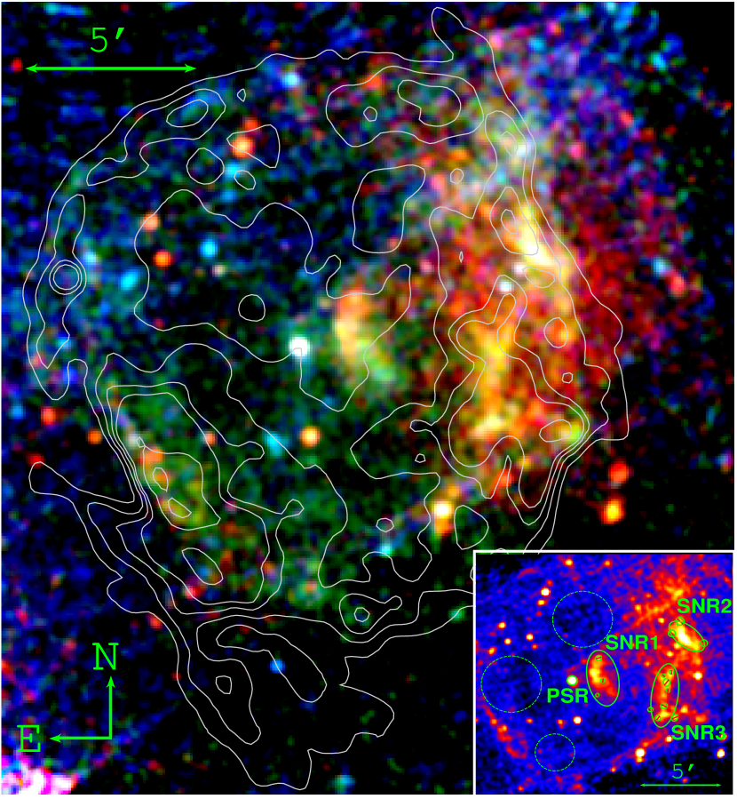
Figure 1.— Three-color image of PSR J1119$-$6127 and G292.2$-$0.5 in the 0.3–1.5 keV (red), 1.5–3 keV (green), and 3–8 keV (blue) bands, made with all XMM-Newton PN and MOS data listed in Table 1 with a total exposure of 100 ks. The image is exposure-corrected, smoothed to 13″ resolution, and overlaid with 1.4-GHz radio contours from Crawford et al. (2001). Inset: intensity map in the 0.3–8 keV band, indicating the source and background extraction regions for the spectral analysis.

3.2. Timing

The timing analysis was carried out with the PN data only, since only they have sufficiently high-time resolution. We extracted source events from a circular aperture of 18″ radius centered on the pulsar. This radius was determined by the tool eregionanalyse to yield the optimal signal-to-noise ratio. We followed Gonzalez et al. (2005) to correct for a timing anomaly in the 2003 data; we did not find any other such anomaly in the other observations. We divided the data into low-energy (0.5–2.5 keV) and high-energy (2.5–8 keV) bands, and obtained $889\pm 30$ and $414\pm 20$ total counts, respectively, with $\sim 110$ and 120 background counts, respectively, as estimated from nearby regions. The event arrival times were first corrected to the solar system barycenter, then folded according to the radio ephemerides. We used the published pulsar ephemeris from Weltevrede et al. (2011) for the 2003 data, while the ephemeris in 2011 was obtained from contemporaneous radio observations with the Parkes radio telescope, as part of the timing program for Fermi (Weltevrede et al., 2010).

First, we verified that the pulse profiles in 2003 and 2011 were consistent. They were subsequently co-added in the analysis to boost the signal-to-noise ratio. The resulting profile is shown in Figure 2. The pulsar emission below 2.5 keV is highly modulated. It exhibits a single-peaked profile with good alignment with the radio pulse. A sinusoid provides an adequate fit to the profile and it gives an rms pulsed fraction (PF) of $0.38\pm 0.03$. To compare with previous work, we follow Gonzalez et al. (2005) and calculate the “max–min PF” using PF=$(F_{\rm max}-F_{\rm min})/(F_{\rm max}+F_{\rm min})$, where $F_{\rm max}$ and $F_{\rm min}$ are the maximum and minimum background-subtracted counts in the binned profile, respectively. In this way, we obtain max–min PF of $0.48\pm 0.12$ in the 0.5–2.5 keV range. This is somewhat lower than the value $0.74\pm 0.14$ reported by Gonzalez et al. (2005), and the discrepancy could be attributed to Poisson fluctuations or to difference in phase binning. On the other hand, no pulsations are detected above 2.5 keV. This is consistent with the findings of Gonzalez et al. (2005) and with the RXTE results in the 2–60 keV range reported by Parent et al. (2011). We place put an upper limit of PF $<10\%$ in the 2.5–8 keV range.

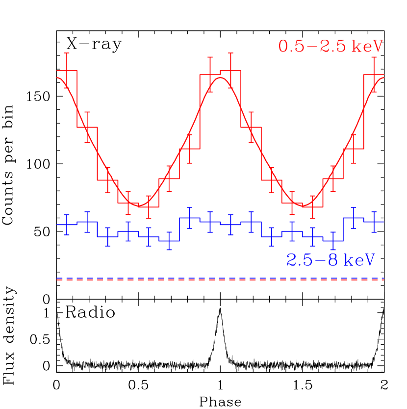
Figure 2.— X-ray pulse profiles of PSR J1119$-$6127 from XMM-Newton PN observations in 0.5–2.5 keV (red) and 2.5–8 keV (blue). The solid line shows the model lightcurve of the soft X-ray emission from a single hot spot with a magnetized atmosphere (see Section 4.1.1). Background levels are indicated by the dashed lines. Phase 0 corresponds to the radio pulse at 1.4 GHz shown in the lower panel. The radio flux density is in an arbitrary unit.

3.3. Spectroscopy

We carried out the spectral analysis with XSPEC 12.7.1. Spectra were grouped to at least 20 counts per bin, and only single and double events (i.e. PATTERN $\leq$ 4) were used for the PN data to ensure the best spectral calibration. We restricted the fits in the 0.5–8 keV. A photoelectric absorption model tbabs by Wilms et al. (2000) was employed throughout our study, and we adopted the abundances given by the same authors.

3.3.1 Phase-averaged Pulsar Spectroscopy

Spectra of PSR J1119$-$6127 were extracted from 18″-radius apertures from the XMM-Newton and Chandra data. Background spectra were extracted from nearby regions free from SNR emission shown in Figure 1. We have also tried using annular background regions centered on the pulsar, and the results are very similar. There are $1062\pm 37$, $500\pm 25$, $442\pm 24$, and $908\pm 35$ net pulsar counts in 0.5–8 keV from the PN, MOS1, MOS2, and ACIS detectors, respectively. A comparison of different spectra shows no variability between epochs. Therefore, we performed a joint fit to all the data. Given the low number of source counts, we did not attempt to account for the cross-calibration uncertainty between instruments (see Tsujimoto et al., 2011).

To account for the PWN contamination, we employed a PWN component in the spectral model, which was extracted from the Chandra data using an annular aperture of 2.5″–18″. We fitted the PWN spectrum using an absorbed power-law (PL) model with the column density ($N_{\rm H}$) fixed at the pulsar value. The PWN component was then held fixed during the fit of the pulsar spectrum. Once a new value of $N_{\rm H}$ was determined, we re-fit the PWN spectrum and the whole process was carried out iteratively until consistent spectral parameters were found. We first tried simple models, including an absorbed blackbody (BB) and an absorbed PL for the pulsar spectrum. However, they fail to describe the data, and we found that an absorbed BB+PL model provides a much better fit ($\chi^{2}_{\nu}=0.97$). This gives a high effective temperature of $kT=0.21\pm 0.04$ keV with a emission radius of $3^{+4}_{-1}$ km (for a source distance of 8.4 kpc), and a PL photon index of $2.1\pm 0.8$. The BB component has an absorbed flux of $1.2\pm 0.3\times 10^{-14}$ erg cm^-2 s^-1 in the 0.5–8 keV energy range, and the non-thermal components have absorbed fluxes of $2.3\pm 0.4\times 10^{-14}$ erg cm^-2 s^-1 and $2.8\times 10^{-14}$ erg cm^-2 s^-1 from the pulsar and the PWN, respectively. The best-fit parameters are listed in Table 2 and the PN spectrum is shown in Figure 3(a).

Following previous studies, we also tried fitting the pulsar spectra with a neutron star atmosphere model (NSA; Zavlin et al., 1996) plus a PL model. The former describes a fully ionized hydrogen atmosphere in a $B$-field of $10^{13}$ G. During the fits, the stellar mass was fixed at 1.4$M_{\odot}$ and we assumed uniform thermal emission over the entire surface of 13 km radius. This yields a fit that is equally as good as the BB+PL model, but with a significantly lower surface temperature of $0.08^{+0.03}_{-0.02}$ keV. The flux normalization suggests a distance of $2.4_{-1.8}^{+5.6}$ kpc, which is lower than the source distance of 8.4 kpc. Table 2 summarizes the best-fit parameters of the BB+PL and NSA+PL fits. All uncertainties quoted are at the 90% confidence level. The parameters are fully consistent with previous studies (Gonzalez et al., 2005; Safi-Harb & Kumar, 2008), and are better constrained in our case. For the case of magnetars, BB+PL spectra are often observed (e.g., Ng et al., 2011) and the PL component is interpreted as magnetospheric upscattering of thermal photons from the surface emission (Thompson et al., 2002). To check if this is the case for PSR J1119$-$6127, we fitted the pulsar spectra with a resonant cyclotron scattering model (RCS; Rea et al., 2008), but obtained very poor results ($\chi^{2}_{\nu}\approx 2$), mainly because the model provides too little flux above 3 keV to account for the observed hard X-ray tail.

Table 2Best-fit Blackbody Plus Power-law (BB+PL) and Neutron Star Atmosphere Plus Power-law (NSA+PL) Models to the Phase-averaged Spectrum of PSR J1119$-$6127

Parameter	BB+PL	NSA+PL
$N_{\rm H}$ ($10^{22}$ cm-2)	$2.2^{+0.5}_{-0.4}$	$2.5^{+0.6}_{-0.5}$
$kT^{\infty}$ (keV)	$0.21\pm 0.04$	$0.08_{-0.02}^{+0.03}$
$R^{\infty}$ (km)	$3_{-1}^{+4}$	13
Distance (kpc)	8.4	$2.4_{-1.8}^{+5.6}$
$\Gamma_{\rm PSR}$	$2.1\pm 0.8$	$2.1\pm 0.8$
$\Gamma_{\rm PWN}$	1.31	1.46
$f_{\rm bb/nsa}^{\rm abs}$ ($10^{-14}$ erg cm-2 s-1)	$1.2\pm 0.3$	$1.4_{-0.3}^{+0.2}$
$f_{\rm bb/nsa}^{\rm unabs}$ ($10^{-14}$ erg cm-2 s-1)	$16_{-7}^{+16}$	$43_{-25}^{+97}$
$f_{\rm pl}^{\rm abs}$ ($10^{-14}$ erg cm-2 s-1)	$2.3\pm 0.4$	$2.3\pm 0.4$
$f_{\rm pl}^{\rm unabs}$ ($10^{-14}$ erg cm-2 s-1)	$5_{-2}^{+6}$	$5_{-2}^{+5}$
$f_{\rm PWN}^{\rm abs}$ ($10^{-14}$ erg cm-2 s-1)	2.8	2.7
$f_{\rm PWN}^{\rm unabs}$ ($10^{-14}$ erg cm-2 s-1)	4.0	4.3
$\chi^{2}_{\nu}$/dof	0.97/161	0.97/161

Note. — All uncertainties are 90% confidence intervals (i.e., 1.6$\sigma$). $f^{\rm abs}$ and $f^{\rm unabs}$ are the absorbed and unabsorbed fluxes, respectively, in the 0.5–8 keV energy range.

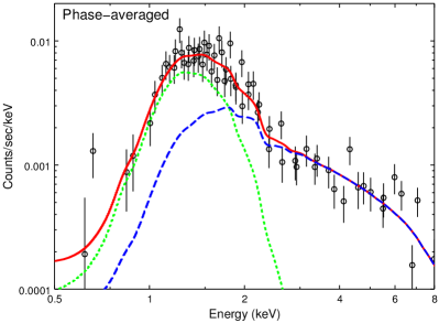
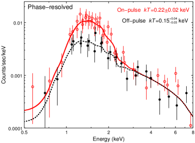
Figure 3.— Top: best-fit blackbody plus power-law model for the phase-averaged spectrum of PSR J1119$-$6127. The thermal component is shown by the dotted green line and the non-thermal component, which composes of pulsar and PWN emission, is shown by the dashed blue line. Only the PN spectra are shown for clarity. Bottom: on-pulse (red open circle) and off-pulse (black filled circle) PN spectra of the pulsar, fitted with the blackbody plus power-law model. See Section 3.3.2 for details.

3.3.2 Phase-resolved Pulsar Spectroscopy

To understand the nature of the X-ray pulsations, we performed phase-resolved spectroscopy using the PN data. Based on the pulse profile in Figure 2, we extracted the off-pulse spectra from phase 0.25–0.75, and the on-pulse spectra from the rest of the phase range. There are $673\pm 29$ and $385\pm 23$ net counts for the on- and off-pulse emission, respectively, in the 0.5–8 keV energy range. The spectra were grouped with at least 20 counts per bin, and fitted to the BB+PL model in the 0.5–8 keV range. As shown in Figure 3(a), the pulsar emission above 2.5 keV is dominated by non-thermal emission, which shows no pulsations (see Figure 2). Therefore, the non-thermal components (from both the pulsar and the PWN) were held fixed at the phase-averaged values during the fits. We also fixed the absorption column density at the best-fit phase-averaged value of $N_{\rm H}=2.2\times 10^{22}$ cm^-2. We note that the non-thermal flux is not enough to account for the off-pulse emission, suggesting the presence of thermal emission at pulse minimum. We found a higher BB temperature of $kT=0.22\pm 0.02$ keV with an effective radius of $R=3.0^{+1.0}_{-0.8}$ km for the on-pulse emission. The off-pulse emission shows a hint of a lower temperature of $kT=0.15^{+0.04}_{-0.03}$ keV and a larger radius of $7_{-7}^{+13}$ km. The best-fit spectral models are shown in Figure 3(b). We have also tried fitting the difference spectrum between on- and off-pulse emission. While it is consistent with a BB model, there are large uncertainties in the spectral parameters due to poor data quality.

Table 3Best-fit PSHOCK Plus Power-law (PS+PL) and Two-temperature PSHOCK (PS+PS) Models for the Spectra of SNR G292.2$-$0.5

	Region 1			Region 2			Region 3
Parameter	PS+PL	PS+PS		PS+PL	PS+PS		PS+PL	PS+PS
$N_{\rm H}$ ($10^{22}$ cm-2)	$2.17^{+0.07}_{-0.08}$	$2.17^{+0.10}_{-0.08}$		$1.9_{-0.2}^{+0.5}$	$0.9\pm 0.2$		$1.15^{+0.07}_{-0.03}$	$1.0\pm 0.1$
$kT_{1}$ (keV)	$0.18\pm 0.02$	$0.18^{+0.3}_{-0.2}$		$0.11^{+0.05}_{-0.02}$	$0.74^{+0.11}_{-0.03}$		$0.66^{+0.03}_{-0.02}$	$0.66\pm 0.03$
$\tau_{1}$ ($10^{10}$ s cm-3)	$40_{-20}^{+40}$	$90_{-40}^{+90}$		$>150$	$>30$		$>200$	$>100$
EM1 ($10^{56}$ cm-3)	$360_{-140}^{+200}$	$330^{+160}_{-120}$		$1100^{+3000}_{-400}$	$0.5\pm 0.2$		$1.9^{+0.4}_{-0.5}$	$1.5^{+0.6}_{-0.4}$
$\Gamma$	$2.9\pm 0.1$	$\cdots$		$3.5^{+0.2}_{-0.1}$	$\cdots$		$3.5\pm 0.2$	$\cdots$
$kT_{2}$ (keV)	$\cdots$	$1.8^{+0.2}_{-0.1}$		$\cdots$	$1.8\pm 0.2$		$\cdots$	$1.0\pm 0.1$
$\tau_{2}$ ($10^{10}$ s cm-3)	$\cdots$	$<0.2$		$\cdots$	$<0.08$		$\cdots$	$<0.08$
EM2 ($10^{56}$ cm-3)	$\cdots$	$4.2^{+0.4}_{-0.6}$		$\cdots$	$2.2\pm 0.3$		$\cdots$	$4.2^{+0.8}_{-0.7}$
$f_{1}^{\rm abs}$	$0.64\pm 0.03$	$0.45\pm 0.02$		$0.15^{+0.04}_{-0.03}$	$0.22^{+0.07}_{-0.06}$		$0.51\pm 0.08$	$0.48^{+0.09}_{-0.08}$
$f_{1}^{\rm unabs}$	$330^{+100}_{-80}$	$300^{+110}_{-80}$		$330^{+700}_{-150}$	$1.1^{+0.8}_{-0.5}$		$3.5^{+0.9}_{-0.8}$	$2.9^{+1.0}_{-0.8}$
$f_{2}^{\rm abs}$	$1.46\pm 0.06$	$1.3^{+0.07}_{-0.05}$		$1.5\pm 0.05$	$0.88\pm 0.08$		$0.73_{-0.09}^{+0.10}$	$0.72^{+0.08}_{-0.09}$
$f_{2}^{\rm unabs}$	$6^{+0.6}_{-0.5}$	$7^{+7}_{-4}$		$6^{+2}_{-1}$	$1.8^{+0.9}_{-0.1}$		$3.7\pm 0.7$	$2.1^{+1.8}_{-0.2}$
$\chi^{2}_{\nu}$/dof	1.21/1175	1.21/1174		1.19/363	1.18/362		1.35/782	1.31/781

Note. — The subscripts 1 and 2 correspond to the soft and hard components, respectively. All uncertainties are 90% confidence intervals (i.e. 1.6$\sigma$). The volume emission measure is given by $\mathrm{EM}=\int n_{e}n_{\rm H}\,{\rm d}V$, where $n_{e}$ and $n_{\rm H}$ are shocked electron and hydrogen number densities, respectively. $\tau=n_{e}t$ is the ionization timescale. The absorbed and unabsorbed fluxes ($f^{\rm abs}$ and $f^{\rm unabs}$) are estimated from the XMM-Newton data, in units of $10^{-13}$ erg cm^-2 s^-1 in the 0.5–8 keV energy range.

3.3.3 SNR Spectroscopy

We extracted spectra of SNR G292.2$-$0.5 from the three brightest regions (see Figure 1) from the XMM-Newton and Chandra data. Our region 1 roughly corresponds to the “east” region in Gonzalez & Safi-Harb (2005), and regions 2 and 3 correspond to their “west” region. Point sources inside these regions were identified and excluded based on the exposure-corrected Chandra and XMM-Newton images. We note that region 2 is not covered by any Chandra observations, therefore, only the XMM-Newton spectra are used in this case. Similarly, only one Chandra exposure is useful for region 3. Since the SNR covers a large part of the Chandra and XMM-Newton PN field of view, we estimated the background spectra using the blank-sky data provided by the calibration teams (Carter & Read, 2007), which were taken from nearby regions in the Galactic plane. We also tried extracting the background spectra from source-free regions far off-axis in our observations and obtained similar results, although this way the sky background tends to be underestimated due to vignetting. After background subtraction, we obtained $1.1\times 10^{4}$ XMM-Newton counts and 5300 Chandra counts for region 1, 4900 XMM-Newton counts for region 2, and 7900 XMM-Newton counts and 2000 Chandra counts for region 3 in 0.5–7.5 keV range.

Emission lines are found in all the spectra, albeit rather weak, indicating a thermal origin for the emission. For each region, we performed a joint fit to the spectra with all parameters linked, and we introduced a constant scaling factor between the XMM-Newton and Chandra spectra to account for the cross-calibration uncertainty (Tsujimoto et al., 2011). We first tried the spectral parameters reported by Gonzalez & Safi-Harb (2005), but these gave very poor fits. Using a non-equilibrium ionization thermal model (PSHOCK; Borkowski et al., 2001) with solar abundances, we obtained reasonable results ($\chi^{2}_{\nu}=$1.3–1.5). The fits can be further improved by allowing the abundances to vary (with the VPSHOCK model) or by adding a hard component, and the improvements are statistically significant as indicated by $F$-tests. However, since the emission lines are weak, the VPSHOCK fits require rather low abundances (0.1–0.5) for all elements between Ne and Fe. Therefore, we believe that a two-component model could be a more physical description of the thermal emission. In this case, the hard component can be described by either a non-thermal PL with photon indices $\Gamma=2.9$–3.5 or by a high temperature ($kT=1$–1.8 keV) PSHOCK model with very low ionization timescales ($\tau\lesssim 10^{9}$ s cm^-3) and solar abundances, and they provide the best fits overall ($\chi^{2}_{\nu}\approx$1.2). The results are listed in Table 3 and the best-fit two-temperature models are plotted in Figure 4. In all the fits, the soft component has a large ionization timescales ($\tau\gtrsim 10^{12}$ s cm^-3). The Chandra flux is $\sim 30$% higher than the XMM-Newton flux, which is not atypical (see Tsujimoto et al., 2011).

4. Discussion

In the following discussion, we adopt a source distance of 8.4 kpc and an age of 1.9 kyr. Although the true age of the system could be different than the pulsar’s characteristic age, we stress that our discussion should remain qualitatively valid for a system age younger than a few thousand years.

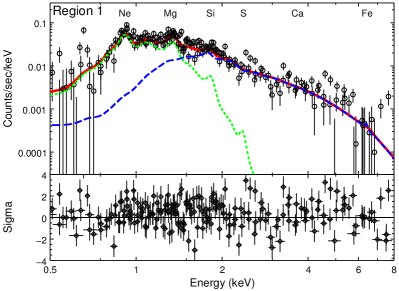
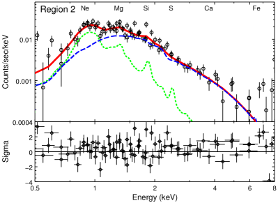
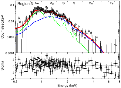
Figure 4.— Best-fit two-temperature PSHOCK models to the spectra of SNR G292.2$-$0.5. The high- and low-temperature components are indicated by the dashed blue lines and dotted green lines, respectively. For clarity, only the PN spectra are shown and all spectra are grouped with a minimum of 50 counts per bin.

4.1. PSR J1119$-$6127

4.1.1 Thermal Emission

PSR J1119$-$6127 is among the youngest radio pulsars with thermal emission detected. As indicated in Figure 3(a), the pulsar flux below 2.5 keV is mostly thermal, and it is highly pulsed and shows good phase alignment with the radio pulse (Figure 2). Combining these two results suggests that the thermal emission could be dominated by a single hot spot near the magnetic pole. Further support for this picture is provided by the phase-resolved spectroscopy, which suggests a hint of a higher temperature for the on-pulse emission than the off-pulse emission (Figure 3(b)). The BB+PL fit to the phase-averaged spectrum gives a high temperature of $0.21\pm 0.04$ keV ($=2.4\pm 0.5$ MK) with an emission radius of $3^{+4}_{-1}$ km, implying a bolometric luminosity of $1.9^{+1.9}_{-0.8}\times 10^{33}$ erg s^-1 for the thermal emission. The BB temperature and luminosity are among the highest of radio pulsars, even when compared to objects with similar age (see Olausen et al., 2010; Ng & Kaspi, 2011; Zhu et al., 2011). Since the stellar surface temperature is non-uniform, the NSA fits only give the average temperature and it cannot be directly compared to the BB temperature. Indeed, the bolometric luminosity above is equivalent to that of a 13 km radius star with a uniform temperature of 0.096 keV (=1.1 MK), comparable to the best-fit NSA temperature of $0.08^{+0.03}_{-0.02}$ keV.

Gonzalez et al. (2005) and Safi-Harb & Kumar (2008) pointed out that the BB luminosity and radius are too large to be reconciled with polar cap heating by return currents from the magnetosphere. Hence, the thermal emission is likely from cooling and its unusual properties, e.g. high temperature and large modulation, could be related to the strong magnetic field of PSR J1119$-$6127. Pons et al. (2007) noticed an apparent correlation between the BB temperature $T$ and the dipole $B$-field $B_{d}$ of neutron stars, with $T\propto\sqrt{B_{d}}$ spanning over three orders of magnitude in $B_{d}$, from radio pulsars to magnetars. They attributed this to crustal heating by magnetic field decay, and subsequently studied the “magneto-thermal evolution” of neutron stars (Aguilera et al., 2008a, b; Pons et al., 2009). In their model, heating from field decay increases the magnetic diffusivity and thermal conductivity of the crust, which in turn accelerates the field decay. As a result, neutron stars born with initial $B$-fields $>5\times 10^{13}$ G could have a surface temperature well above the minimal cooling scenario (Aguilera et al., 2008a; Kaminker et al., 2009).

The thermal emission of PSR J1119$-$6127 offers an interesting test case for the above theory. While the BB temperature we obtained is comparable to the predicted value at the pole (Aguilera et al., 2008a), the bolometric luminosity of $\sim 10^{33}-10^{34}$ erg s^-1 could be easily explained by passive cooling (e.g. Page et al., 2004), thus, providing no evidence for energy injection from $B$-field decay. Indeed, the higher temperature at the pole could be attributed to anisotropic heat conduction. Since free electrons, which are the main heat carriers, are confined to the magnetic field lines, heat transport perpendicular to the field is strongly suppressed (Greenstein & Hartke, 1983). This acts as a “heat blanket” at the magnetic equator, while the magnetic poles are in thermal equilibrium with the core. As a result, the surface temperature distribution is non-uniform with warmer spots at the magnetic poles separated by cooler regions at lower magnetic latitude (e.g. Geppert et al., 2004; Shabaltas & Lai, 2012).

It is believed that the internal magnetic field of a neutron star likely consists of a toroidal component, which could be generated by differential rotation that wraps the poloidal field in a proto-neutron star (e.g. Thompson & Duncan, 1993). Geppert et al. (2006) showed that the presence of a toroidal $B$-field in the crust could further suppress the heat transport from the core towards the magnetar equator, because that requires crossing the toroidal field lines. As a result, this would enhance the heat blanket effect. Moreover, since the toroidal field component is symmetric about the magnetic equator but the poloidal component is antisymmetric, the total $B$-field would be asymmetric. Hence, the thermal emission from one magnetic pole could dominate over another, which could help explain the single-peaked pulse profile we found. Furthermore, the PF could be boosted by effects of limb-darkening and magnetic beaming in the neutron star atmosphere (e.g., Pavlov et al., 1994; Rajagopal et al., 1997; van Adelsberg & Lai, 2006). Magnetic beaming is due to anisotropic scattering and absorption of photons in magnetized plasmas. The resulting radiation from a hot spot consists of a narrow pencil beam $<5\arcdeg$ along the magnetic field and a broad fan beam at intermediate angles of 20°–60° (Zavlin et al., 1995; van Adelsberg & Lai, 2006).

To test these ideas, we employed a magnetized partially ionized hydrogen atmosphere model (Ho et al., 2008), which accounts for the magnetic and relativistic effects, to generate X-ray spectra and pulse profiles with a similar procedure as Ho (2007). We took a surface $B$-field of $4\times 10^{13}$ G and surface redshift of $1+z=1.19$, and adopted the viewing geometry of magnetic inclination angle $\alpha\approx 125\arcdeg$ and spin-axis inclination angle $\zeta\approx 145\arcdeg$ obtained from modeling of the pulsar $\gamma$-ray lightcurve and radio polarization profile (Parent et al., 2011). Vacuum polarization is ignored here, since it is not important for the total surface emission at this field strength (van Adelsberg & Lai, 2006). We tried different model parameters and found that two identical antipodal hot spots give a very low PF of $\sim 5$%. The observed single-peaked pulse profile can be produced if the temperature of one hot spot is higher than the other. Our best-fit model is given by a hot spot with effective temperature (observed at infinity) of $kT=0.13$ keV (i.e. 1.5 MK) and an area of one third of the stellar surface, and for the other hot spot, we place a temperature upper limit of 0.08 keV assuming a similar area. This is shown by the solid line in Figure 2. This temperature is lower than the best-fit BB temperature for the on-pulse spectrum (see Figure 3(b)) and also the emitting area here is larger. These are typical characteristics of an atmosphere model when compared to a simple BB, since non-gray opacities in the former cause higher energy photons to be seen from deeper and hence hotter layers in the atmosphere (e.g. Romani, 1987; Shibanov et al., 1992). Note that the model suggests a rather large emitting area. This is because given the viewing geometry, the observer’s line of sight would cut through the fan beam twice during one rotation. Therefore, a much smaller hot spot would produce a double-peaked pulse profile. Finally, our model predicts a decreasing “max–min PF” with energy, from 0.5 at 0.5 keV to 0.4 at 2 keV, however, this difference is too small to be detected given our data quality. Deeper observations are needed to confirm this.

As a caveat, we note that the viewing geometry obtained from the $\gamma$-ray lightcurve is model dependent. If the constraints on $\alpha$ and $\zeta$ are relaxed, the high PF could also be explained by some extreme viewing geometries, such that only one pole is observable (see Gonzalez et al., 2005).

Table 4High-$B$ Radio Pulsars with Detected Pulsed Thermal Emission

Name	$P$	$B$	$\tau_{c}$	Distance	$kT$	$L_{\rm bol}$	PF	Reference
	(s)	($10^{13}$ G)	(kyr)	(kpc)	(keV)	($10^{32}$ erg s-1)
J1119$-$6127	0.41	4.1	1.7	8.4	$0.21\pm 0.04$	$19^{+19}_{-8}$	$0.48\pm 0.12$	This work
J1819$-$1458	4.3	5.0	117	$\sim$3.6	$0.12\pm 0.02$	$1.2^{+2}_{-0.8}$	$0.37\pm 0.05$	1
J1718$-$3718	3.4	7.4	34	$\sim$4.5	$0.19\pm 0.02$	$4^{+5}_{-2}$	$0.60\pm 0.13$	2

Note. — The characteristic ages ($\tau_{c}$) are inferred from the spin parameters. $kT$ are the best-fit blackbody temperatures. The pulsed fractions (PF) are estimated with the “max–min PF” (see the text) in 0.5–2.5 keV, 0.3–5 keV, and 0.8–2 keV for PSRs J1119$-$6127, J1819$-$1458, and J1718$-$3718, respectively.

References. — (1) Rea et al. 2009; (2) Zhu et al. 2011.

4.1.2 Non-thermal Emission

The X-ray spectrum of PSR J1119$-$6127 clearly shows a PL component with a photon index of $\Gamma=2.1\pm 0.8$ and an unabsorbed flux of $5^{+6}_{-2}\times 10^{-14}$ erg cm^-2 s^-1 in the 0.5–8 keV range. Since the RCS model gives a poor fit, this seems unlikely to be up-scattering of thermal photons as in magnetars. We believe that it could be synchrotron radiation originated from the PWN or from the pulsar magnetosphere. Assuming constant surface brightness, the PWN would provide an unabsorbed flux of only $8\times 10^{-16}$ erg cm^-2 s^-1 in the 0.5–8 keV range in the central 2$\farcs$5-radius region. However, the actual PWN contribution is likely to be higher, since compact PWN emission is often found to be peaked toward the pulsar (see Ng & Romani, 2008). Deeper Chandra observations are needed to determine if the PL photon indices of the pulsar and PWN components are consistent. In addition to PWN emission, young rotation-powered pulsars generally show strong magnetospheric emission in X-rays (e.g. Ng et al., 2008a). However, this emission is expected to be highly pulsed (Zhang & Cheng, 2002), which is not observed in our case. At a distance of 8.4 kpc, the non-thermal emission we found has a luminosity of $L_{X}=4.2\times 10^{32}$ erg s^-1 (0.5–8 keV), a few times larger than the flux $8.5\times 10^{31}$ erg s^-1 suggested by Zhang & Jiang (2005) based on the outergap model.

4.1.3 Connection with Other High-$B$ Pulsars and Magnetars

Among all high-$B$ radio pulsars listed in Ng & Kaspi (2011), only four (PSRs J1119$-$6127, J1819$-$1458, J1718$-$3718, and J1846$-$0258) are bright enough to have X-ray pulsations detected. Except PSR J1846$-$0258, which has a purely non-thermal spectrum (Gotthelf et al., 2000; Ng et al., 2008a), the rest show thermal emission with high BB temperature around 0.1–0.2 keV. We summarize their timing and spectral properties in Table 4.1.1. Interestingly, their X-ray pulse profiles are all single-peaked and well aligned with the radio pulse, and show large modulations with PFs from 40% to 60%. These striking similarities suggest that the physics we discussed above in Section 4.1.1 could be applicable to other high-$B$ pulsars. More X-ray observations are needed to confirm this idea. In particular, PSRs J1734$-$3333 and B1916+14, which are detected in X-rays but for which no pulsations have yet been found (Olausen et al., 2012; Zhu et al., 2009; Olausen et al., 2010), would be ideal targets.

PSR J1846$-$0258 is a very special object in the class, as it has shown magnetar-like activity, including short X-ray bursts (Gavriil et al., 2008) accompanied by a glitch with unusual recovery properties (Livingstone et al., 2010, 2011). This led to speculation that high-$B$ radio pulsars could be magnetars in quiescence. It has been proposed that radio pulsars and magnetars could be a unified class of objects (Kaspi & McLaughlin, 2005; Perna & Pons, 2011) and high-$B$ pulsars could exhibit magnetar-like bursting behavior, albeit less frequently ($\sim$1 per century). Radio timing of PSR J1119$-$6127 revealed a glitch in 2007 that induced abnormal radio emission (Weltevrede et al., 2011). It is unclear if the pulsar exhibited any X-ray variability at the same time, due to the lack of sensitive X-ray monitoring. Our XMM-Newton observations in 2011 are not useful, since the post-outburst flux relaxation timescale is likely shorter than a few years (e.g. Livingstone et al., 2011). This highlights the importance of X-ray monitoring or rapid post-glitch follow-up in the study of high-$B$ radio pulsars and magnetars.

4.2. SNR G292.2$-$0.5

4.2.1 SNR Environment and Evolution

We have carried out spectral analysis of three brightest regions in SNR G292.2$-$0.5. The spectra are well-described by absorbed two-component models. While the best-fit absorption column densities of the pulsar and region 1 are consistent ($\sim 2\times 10^{22}\,\mathrm{cm}^{-2}$), the values are lower for regions 2 and 3 ($\sim 1\times 10^{22}\,\mathrm{cm}^{-2}$). These seem to suggest an east-west gradient of $N_{\rm H}$ across the field. This is more evident in the three-color image in Figure 1: the western part of the SNR is redder than the eastern part, indicating a softer spectrum which could be due to a lower absorption. This trend is consistent with previous findings (Pivovaroff et al., 2001; Gonzalez & Safi-Harb, 2005; Gonzalez et al., 2005; Safi-Harb & Kumar, 2008), and can be attributed to a dark molecular cloud DC 292.3$-$0.4 to the east of the pulsar as first proposed by Pivovaroff et al. (2001).

The SNR emission consists of a soft thermal component with $kT<1$ keV and a hard component that can be described either by a non-thermal PL of photon index $\Gamma=2.9-3.5$ or by high temperature non-equilibrium ionization plasma with $kT=1-2$ keV. While non-thermal synchrotron emission is often observed in young SNRs, the PL photon index we found ($\Gamma\sim 3.5$) is higher than the typical values of 2–3 in other systems (see a review by Reynolds, 2008). In addition, the fit statistics are slightly worse than that of the two-temperature model. These seem to suggest that the latter may be a more plausible model. In this case, the solar abundances of the high-temperature plasma suggest a circumstellar or interstellar origin, hence, the reverse shock probably has not yet propagated through the ejecta. Together with the high temperature and small ionization timescales, these provide support for the young age of the system. The emission measure could give us a handle on the ambient density $n_{0}$. Assuming a slab geometry for the emitting regions with thickness equal to the width, and taking an electron-to-proton density ratio of 1.2 and a shock compression ratio of 4, we obtained $n_{0}\sim 0.1$ cm^-3 in all three regions. The low-temperature component, however, is more difficult to interpret. Following the same calculation, we estimate $n_{0}$ of 0.6, 0.03, and 0.07 cm^-3 in regions 1, 2, and 3, respectively. This could suggest dense clump for region 1. For regions 2 and 3, a comparison to the large ionization timescales ($\tau\gtrsim 10^{12}$ s cm^-3) indicates that the plasma could have been shocked $\sim 10^{5}$ yr ago, which seems difficult to reconcile with the SNR emission. As we suggest below, the emission may arise from the progenitor wind interaction with the surrounding.

At a distance of 8.4 kpc, the 8$\farcm$5-radius SNR shell has a physical size of 21 pc (Caswell et al., 2004). Such a large radius at a young age requires a high average expansion rate of $v_{s}=21\,\mathrm{pc/1.9\,kyr}=1.1\times 10^{4}$ km s^-1. If this is the present-day shock velocity, then the proton temperature would be $kT_{p}=0.11m_{\rm H}v_{s}^{2}=130$ keV, where $m_{\rm H}$ is the proton mass, and an adiabatic index of $\gamma=5/3$ and cosmic abundances (i.e., 90% H and 10% He) are assumed. A comparison to the best-fit $kT\approx 1$ keV implies an electron-to-proton temperature ratio of $\sim 0.01$, lower than in most SNRs observed (see van Adelsberg et al., 2008). If the ambient medium has a uniform density of $n_{0}\approx 0.1\,\mathrm{cm}^{-3}$ as estimated above, then the swept-up mass would be $\sim 100\,M_{\odot}$, much larger than the typical ejecta mass of $\lesssim 10M_{\odot}$. Hence, the remnant could be in a transition to the adiabatic phase. Based on the Sedov solution, Crawford et al. (2001) derived a constraint on the ratio between $n_{0}$ (in cm^-3) and the explosion energy $E_{51}$ in units of $10^{51}$ erg. The updated distance and age estimates from Caswell et al. (2004) and Weltevrede et al. (2011) imply $E_{51}/n_{0}=200$, requiring an exceptionally large explosion energy or a very low ambient density. It has been proposed that a newborn neutron star with magnetar-like $B$-field ($\sim 10^{15}$ G) and a short spin period ($\sim 1$ ms) would spin down quickly via magnetic braking. As a result, the huge amount of rotational energy released ($\sim 10^{52}$ erg) could accelerate the SNR expansion (Allen & Horvath, 2004). While we cannot rule out this possibility, the explosion energies of three SNRs associated with magnetars (Kes 73, CTB 109, and N49) are found to be close to the canonical value of $10^{51}$ erg (Vink & Kuiper, 2006), which is not consistent with this hypothesis.

As an alternative, the supernova could have occurred in a low-density wind bubble (e.g., Gaensler et al., 1999; Gvaramadze, 2006; Ng et al., 2007). This scenario was briefly mentioned by Caswell et al. (2004) and here we further explore this idea. Chevalier (2005) discussed different types of core collapse supernovae and the properties of their remnants. Type IIP and IIL/b supernovae are the end products of red supergiants (RSGs), which have initial masses $\sim 9-25M_{\odot}$ and $\sim 25-35M_{\odot}$, respectively (Heger et al., 2003), and they are surrounded by dense circumstellar RSG winds extending to a few pc. In contrast, supernovae of Type Ib/c are believed to originate from Wolf-Rayet (WR) progenitors, which are massive stars $\gtrsim 35M_{\odot}$ with high mass-loss rates and high-velocity winds, which are about two orders of magnitudes faster than RSG winds. For a WR star evolved from an RSG, the fast WR wind would sweep up the slow RSG wind ejected earlier to evacuate a low-density wind bubble of radius $\gtrsim 10$ pc over the lifetime $\sim 2\times 10^{5}$ yr of the WR phase (Chevalier, 2005). The swept-up shell is characterized by clumpy structure due to Rayleigh-Taylor instabilities, and overabundance in N and underabundance in C and O (Garcia-Segura et al., 1996).

We argue that SNR G292.2$-$0.5 is unlikely to be a Type IIP or IIL/b supernova because in these cases the remnant should expand into the dense circumstellar RSG winds. A Type Ib/c event with a WR progenitor, one of the possibilities mentioned by Chevalier (2005), therefore seems more likely. In this picture, the SNR had a long free-expansion phase in the low-density wind bubble, with the initial expansion rate up to a few times $10^{4}$ km s^-1, as seen in SN 1987A (Gaensler et al., 1997; Ng et al., 2008b). When the shock reached the cavity boundary at large radius, it began to encounter the clumpy swept-up shell and hence decelerated. The shock interaction then gave rise to the observed hard component in the spectra, either thermal or non-thermal. This scenario may be able to explain the soft component too. The large ionization timescales of the emission are comparable to the lifetime of the WR phase, suggesting that it may originate from the swept-up RSG wind. Two WR bubbles have been detected in X-rays and their spectra can be fitted by a two-temperature thermal model with $kT\sim 0.1$ and 1 keV (Wrigge et al., 2005; Toalá et al., 2012). The high-temperature component is comparable to what we observed for SNR G292.2$-$0.5, while the low-temperature component may be too absorbed to detect in our case. In addition, hydrodynamic simulations and observations suggest a density of $\sim 0.1$ cm^-3 in the hot bubbles (Garcia-Segura et al., 1996; Dwarkadas, 2007; Toalá et al., 2012), which is also consistent with our findings. Deeper X-ray observations in the future can probe the chemical composition of the circumstellar medium to confirm its nature. Moreover, if the SNR is detected in optical wavelengths, then spectral line observations could directly measure the shock velocity to reveal the evolutionary state of the remnant.

4.2.2 Progenitors of High-$B$ Pulsars and Magnetars

In addition to PSR J1119$-$6127, only two other young high-$B$ radio pulsars have associated SNRs detected: PSR J1846$-$0258 in Kes 75 and PSR B1509$-$58 in MSH 15$-$52. Intriguingly, both of them were claimed to have a WR progenitor (Morton et al., 2007; Gaensler et al., 1999). There is also observational evidence hinting at a similar mass range for magnetar progenitors, e.g., 1E 1048.1$-$5937, CXOU J1647$-$4552, and SGR 1806$-$20 (Gaensler et al., 2005; Muno et al., 2006; Figer et al., 2005), although intermediate masses were suggested for two cases: 1E 1841$-$045 and SGR 1900+14 (Chevalier, 2005; Davies et al., 2009). This raises the important question regarding a possible correlation between progenitor mass and neutron star magnetic field. Recently, Chevalier (2011) compared different classes of young neutron stars in SNRs, including magnetars, radio pulsars, and central compact objects, and suggested a tendency for higher $B$-field objects to have more massive progenitors. However, it was noted that other parameters, such as rotation, metallicity, and binarity, likely also play an important role.

The origin of magnetic fields in neutron stars has long been an open problem. Theories suggest that it could be the fossil $B$-fields of the progenitors preserved during core collapse (e.g., Woltjer, 1964; Ruderman, 1972; Ferrario & Wickramasinghe, 2006) or from field amplification via an $\alpha$–$\Omega$ dynamo in rapidly rotating stars (e.g., Duncan & Thompson, 1992; Thompson & Duncan, 1993). A positive correlation between progenitor mass and neutron star $B$-field may be expected in both scenarios (Ferrario & Wickramasinghe, 2008). Massive stars tend to have higher surface $B$-fields (Petit et al., 2008). They also spend less time in the hydrogen and helium burning phases, during which significant braking occurs. Hence, the core could retain a large angular momentum, resulting in efficient dynamo action. If further studies confirm that the progenitors of high-$B$ radio pulsars and magnetars have comparable mass, then no matter which of the above mechanisms is at work, the $B$-fields in these objects could be generated in a similar way. In this respect, magnetars could have the same formation channel as radio pulsars, which would support a unification of these classes of objects (Kaspi & McLaughlin, 2005; Kaspi, 2010; Perna & Pons, 2011).

5. Conclusion

We performed a detailed X-ray study of the young high-$B$ radio pulsar J1119$-$6127 and its associated SNR G292.2$-$0.5 using deep XMM-Newton and Chandra observations. The pulsar emission exhibits strong pulsations below 2.5 keV, with a single-peaked profile that aligns with the radio pulse. Such a single-peaked profile and alignment seem common among thermally emitting high-$B$ pulsars, and we showed that the observed pulsed profile can be modeled by a large hot spot near the magnetic pole. The pulsar spectrum is well fitted by an absorbed BB plus PL model. The BB temperature $kT=0.21\pm 0.04$ keV is highest among young radio pulsars. The thermal emission has a bolometric luminosity of $1.9^{+1.9}_{-0.8}\times 10^{33}$ erg s^-1, which is consistent with neutron star cooling and no heating by $B$-field decay is needed. However, passive magnetic effects, including anisotropic heat conduction and beaming, must play a part in the high temperature and large modulation of the emission.

The spectra of SNR G292.2$-$0.5 are best fitted by a two-component model with solar abundances. The soft component has a thermal origin with $kT\lesssim 1$ keV and a large ionization timescale, while the hard component can be described either by a PL with $\Gamma=2.9-3.5$ or by higher temperature ($kT=1-2$ keV) thermal emission with low ionization. For a young age of 1900 yr inferred from the pulsar’s spin down, the 21 pc SNR shell diameter (at a distance of 8.4 kpc) implies a fast expansion in the past. This could be the result of exceptionally large explosion energy $\gtrsim 10^{52}$ erg or supernova in a wind cavity. We believe that the latter is more plausible, and this could suggest a Type I b/c supernova with a WR progenitor. WR stars have a typical mass $\gtrsim 35\,M_{\odot}$ and they have also been proposed as the progenitors for two other high-$B$ radio pulsars. There is evidence that magnetar progenitors could be in a similar mass range, leading to a speculation that the two classes of neutron stars may have the same formation channel. If confirmed, it will provide a strong support to the idea of unification of these classes of objects.

We note that late in the preparation of this manuscript, we became aware of work (Kumar et al., 2012) on the study of the SNR using the same archival Chandra data and a subset ($\sim 50$ ks) of XMM-Newton data we have used in our study. While our deeper observations gave different spectral parameters for SNR G292.2$-$0.5, we arrived at similar conclusions regarding a possible massive progenitor for PSR J1119$-$6127.

Facilities: CXO (ACIS) XMM (EPIC)

References

- Aguilera et al. (2008a) Aguilera, D. N., Pons, J. A., & Miralles, J. A. 2008a, A&A, 486, 255
- Aguilera et al. (2008b) Aguilera, D. N., Pons, J. A., & Miralles, J. A. 2008b, ApJ, 673, L167
- Allen & Horvath (2004) Allen, M. P., & Horvath, J. E. 2004, ApJ, 616, 346
- Archibald et al. (2008) Archibald, A. M., Kaspi, V. M., Livingstone, M. A., & McLaughlin, M. A. 2008, ApJ, 688, 550
- Borkowski et al. (2001) Borkowski, K. J., Lyerly, W. J., & Reynolds, S. P. 2001, ApJ, 548, 820
- Camilo et al. (2000) Camilo, F., Kaspi, V. M., Lyne, A. G., Manchester, R. N., Bell, J. F., D’Amico, N., McKay, N. P. F., & Crawford, F. 2000, ApJ, 541, 367
- Camilo et al. (2007) Camilo, F., Ransom, S. M., Halpern, J. P., & Reynolds, J. 2007, ApJ, 666, L93
- Camilo et al. (2006) Camilo, F., Ransom, S. M., Halpern, J. P., Reynolds, J., Helfand, D. J., Zimmerman, N., & Sarkissian, J. 2006, Nature, 442, 892
- Carter & Read (2007) Carter, J. A., & Read, A. M. 2007, A&A, 464, 1155
- Caswell et al. (2004) Caswell, J. L., McClure-Griffiths, N. M., & Cheung, M. C. M. 2004, MNRAS, 352, 1405
- Chevalier (2005) Chevalier, R. A. 2005, ApJ, 619, 839
- Chevalier (2011) Chevalier, R. A. 2011, in AIP Conf. Proc., Vol. 1379, Astrophysics of Neutron Stars 2010: A Conference in Honor of M. Ali Alpar, ed. E. Göğüş, T. Belloni, Uuml. Ertan , 5
- Crawford et al. (2001) Crawford, F., Gaensler, B. M., Kaspi, V. M., Manchester, R. N., Camilo, F., Lyne, A. G., & Pivovaroff, M. J. 2001, ApJ, 554, 152
- Davies et al. (2009) Davies, B., Figer, D. F., Kudritzki, R.-P., Trombley, C., Kouveliotou, C., & Wachter, S. 2009, ApJ, 707, 844
- Duncan & Thompson (1992) Duncan, R. C., & Thompson, C. 1992, ApJ, 392, L9
- Dwarkadas (2007) Dwarkadas, V. V. 2007, ApJ, 667, 226
- Ferrario & Wickramasinghe (2006) Ferrario, L., & Wickramasinghe, D. 2006, MNRAS, 367, 1323
- Ferrario & Wickramasinghe (2008) Ferrario, L., & Wickramasinghe, D. 2008, MNRAS, 389, L66
- Figer et al. (2005) Figer, D. F., Najarro, F., Geballe, T. R., Blum, R. D., & Kudritzki, R. P. 2005, ApJ, 622, L49
- Gaensler et al. (1999) Gaensler, B. M., Brazier, K. T. S., Manchester, R. N., Johnston, S., & Green, A. J. 1999, MNRAS, 305, 724
- Gaensler et al. (1997) Gaensler, B. M., Manchester, R. N., Staveley-Smith, L., Tzioumis, A. K., Reynolds, J. E., & Kesteven, M. J. 1997, ApJ, 479, 845
- Gaensler et al. (2005) Gaensler, B. M., McClure-Griffiths, N. M., Oey, M. S., Haverkorn, M., Dickey, J. M., & Green, A. J. 2005, ApJ, 620, L95
- Garcia-Segura et al. (1996) Garcia-Segura, G., Langer, N., & Mac Low, M.-M. 1996, A&A, 316, 133
- Gavriil et al. (2008) Gavriil, F. P., Gonzalez, M. E., Gotthelf, E. V., Kaspi, V. M., Livingstone, M. A., & Woods, P. M. 2008, Science, 319, 1802
- Geppert et al. (2004) Geppert, U., Küker, M., & Page, D. 2004, A&A, 426, 267
- Geppert et al. (2006) Geppert, U., Küker, M., & Page, D. 2006, A&A, 457, 937
- Gonzalez & Safi-Harb (2003) Gonzalez, M., & Safi-Harb, S. 2003, ApJ, 591, L143
- Gonzalez & Safi-Harb (2005) Gonzalez, M., & Safi-Harb, S. 2005, ApJ, 619, 856
- Gonzalez et al. (2005) Gonzalez, M. E., Kaspi, V. M., Camilo, F., Gaensler, B. M., & Pivovaroff, M. J. 2005, ApJ, 630, 489
- Gotthelf et al. (2000) Gotthelf, E. V., Vasisht, G., Boylan-Kolchin, M., & Torii, K. 2000, ApJ, 542, L37
- Greenstein & Hartke (1983) Greenstein, G., & Hartke, G. J. 1983, ApJ, 271, 283
- Gvaramadze (2006) Gvaramadze, V. V. 2006, A&A, 454, 239
- Heger et al. (2003) Heger, A., Fryer, C. L., Woosley, S. E., Langer, N., & Hartmann, D. H. 2003, ApJ, 591, 288
- Ho (2007) Ho, W. C. G. 2007, MNRAS, 380, 71
- Ho (2012) Ho, W. C. G. 2012, MNRAS, in press (arXiv:1208.1297)
- Ho et al. (2008) Ho, W. C. G., Potekhin, A. Y., & Chabrier, G. 2008, ApJS, 178, 102
- Kaminker et al. (2009) Kaminker, A. D., Potekhin, A. Y., Yakovlev, D. G., & Chabrier, G. 2009, MNRAS, 395, 2257
- Kaspi (2010) Kaspi, V. M. 2010, Proceedings of the National Academy of Science, 107, 7147
- Kaspi & McLaughlin (2005) Kaspi, V. M., & McLaughlin, M. A. 2005, ApJ, 618, L41
- Kumar & Safi-Harb (2008) Kumar, H. S., & Safi-Harb, S. 2008, ApJ, 678, L43
- Kumar et al. (2012) Kumar, H. S., Safi-Harb, S., & Gonzalez, M. E. 2012, ApJ, 754, 96
- Levin et al. (2010) Levin, L., et al. 2010, ApJ, 721, L33
- Livingstone et al. (2010) Livingstone, M. A., Kaspi, V. M., & Gavriil, F. P. 2010, ApJ, 710, 1710
- Livingstone et al. (2011) Livingstone, M. A., Ng, C.-Y., Kaspi, V. M., Gavriil, F. P., & Gotthelf, E. V. 2011, ApJ, 730, 66
- Mereghetti (2008) Mereghetti, S. 2008, A&A Rev., 15, 225
- Morton et al. (2007) Morton, T. D., Slane, P., Borkowski, K. J., Reynolds, S. P., Helfand, D. J., Gaensler, B. M., & Hughes, J. P. 2007, ApJ, 667, 219
- Muno et al. (2006) Muno, M. P., et al. 2006, ApJ, 636, L41
- Ng et al. (2008a) Ng, C., Slane, P. O., Gaensler, B. M., & Hughes, J. P. 2008a, ApJ, 686, 508
- Ng et al. (2008b) Ng, C.-Y., Gaensler, B. M., Staveley-Smith, L., Manchester, R. N., Kesteven, M. J., Ball, L., & Tzioumis, A. K. 2008b, ApJ, 684, 481
- Ng & Kaspi (2011) Ng, C.-Y., & Kaspi, V. M. 2011, in AIP Conf. Proc., Vol. 1379, Astrophysics of Neutron Stars 2010: A Conference in Honor of M. Ali Alpar, ed. E. Göğüş, T. Belloni, Uuml. Ertan , 60
- Ng & Romani (2008) Ng, C.-Y., & Romani, R. W. 2008, ApJ, 673, 411
- Ng et al. (2007) Ng, C.-Y., Romani, R. W., Brisken, W. F., Chatterjee, S., & Kramer, M. 2007, ApJ, 654, 487
- Ng et al. (2011) Ng, C.-Y., et al. 2011, ApJ, 729, 131
- Olausen et al. (2010) Olausen, S. A., Kaspi, V. M., Lyne, A. G., & Kramer, M. 2010, ApJ, 725, 985
- Olausen et al. (2012) Olausen, S. A., et al. 2012, ApJ, submitted
- Page et al. (2004) Page, D., Lattimer, J. M., Prakash, M., & Steiner, A. W. 2004, ApJS, 155, 623
- Parent et al. (2011) Parent, D., et al. 2011, ApJ, 743, 170
- Pavlov et al. (1994) Pavlov, G. G., Shibanov, Y. A., Ventura, J., & Zavlin, V. E. 1994, A&A, 289, 837
- Perna & Pons (2011) Perna, R., & Pons, J. A. 2011, ApJ, 727, L51
- Petit et al. (2008) Petit, V., Wade, G. A., Drissen, L., Montmerle, T., & Alecian, E. 2008, MNRAS, 387, L23
- Pivovaroff et al. (2001) Pivovaroff, M. J., Kaspi, V. M., Camilo, F., Gaensler, B. M., & Crawford, F. 2001, ApJ, 554, 161
- Pons et al. (2007) Pons, J. A., Link, B., Miralles, J. A., & Geppert, U. 2007, Physical Review Letters, 98, 071101
- Pons et al. (2009) Pons, J. A., Miralles, J. A., & Geppert, U. 2009, A&A, 496, 207
- Rajagopal et al. (1997) Rajagopal, M., Romani, R. W., & Miller, M. C. 1997, ApJ, 479, 347
- Rea & Esposito (2011) Rea, N., & Esposito, P. 2011, in High-Energy Emission from Pulsars and their Systems, ed. D. F. Torres & N. Rea (Berlin: Springer), 247
- Rea et al. (2008) Rea, N., Zane, S., Turolla, R., Lyutikov, M., & Götz, D. 2008, ApJ, 686, 1245
- Rea et al. (2009) Rea, N., et al. 2009, ApJ, 703, L41
- Rea et al. (2010) Rea, N., et al. 2010, Science, 330, 944
- Reynolds (2008) Reynolds, S. P. 2008, ARA&A, 46, 89
- Romani (1987) Romani, R. W. 1987, ApJ, 313, 718
- Ruderman (1972) Ruderman, M. 1972, ARA&A, 10, 427
- Safi-Harb & Kumar (2008) Safi-Harb, S., & Kumar, H. S. 2008, ApJ, 684, 532
- Scholz et al. (2012) Scholz, P., Ng, C.-Y., Livingstone, M. A., Kaspi, V. M., Cumming, A., & Archibald, R. 2012, ApJ, in press (arXiv:1204.1034)
- Shabaltas & Lai (2012) Shabaltas, N., & Lai, D. 2012, ApJ, 748, 148
- Shibanov et al. (1992) Shibanov, I. A., Zavlin, V. E., Pavlov, G. G., & Ventura, J. 1992, A&A, 266, 313
- Thompson & Duncan (1993) Thompson, C., & Duncan, R. C. 1993, ApJ, 408, 194
- Thompson & Duncan (1995) Thompson, C., & Duncan, R. C. 1995, MNRAS, 275, 255
- Thompson & Duncan (1996) Thompson, C., & Duncan, R. C. 1996, ApJ, 473, 322
- Thompson et al. (2002) Thompson, C., Lyutikov, M., & Kulkarni, S. R. 2002, ApJ, 574, 332
- Toalá et al. (2012) Toalá, J. A., Guerrero, M. A., Chu, Y.-H., Gruendl, R. A., Arthur, S. J., Smith, R. C., & Snowden, S. L. 2012, ApJ, 755, 77
- Tsujimoto et al. (2011) Tsujimoto, M., et al. 2011, A&A, 525, A25
- van Adelsberg et al. (2008) van Adelsberg, M., Heng, K., McCray, R., & Raymond, J. C. 2008, ApJ, 689, 1089
- van Adelsberg & Lai (2006) van Adelsberg, M., & Lai, D. 2006, MNRAS, 373, 1495
- Vink & Kuiper (2006) Vink, J., & Kuiper, L. 2006, MNRAS, 370, L14
- Weltevrede et al. (2011) Weltevrede, P., Johnston, S., & Espinoza, C. M. 2011, MNRAS, 411, 1917
- Weltevrede et al. (2010) Weltevrede, P., et al. 2010, PASA, 27, 64
- Wilms et al. (2000) Wilms, J., Allen, A., & McCray, R. 2000, ApJ, 542, 914
- Woltjer (1964) Woltjer, L. 1964, ApJ, 140, 1309
- Wrigge et al. (2005) Wrigge, M., Chu, Y.-H., Magnier, E. A., & Wendker, H. J. 2005, ApJ, 633, 248
- Zavlin et al. (1996) Zavlin, V. E., Pavlov, G. G., & Shibanov, Y. A. 1996, A&A, 315, 141
- Zavlin et al. (1995) Zavlin, V. E., Pavlov, G. G., Shibanov, Y. A., & Ventura, J. 1995, A&A, 297, 441
- Zhang & Cheng (2002) Zhang, L., & Cheng, K. S. 2002, ApJ, 569, 872
- Zhang & Jiang (2005) Zhang, L., & Jiang, Z. J. 2005, ApJ, 632, 523
- Zhu et al. (2009) Zhu, W., Kaspi, V. M., Gonzalez, M. E., & Lyne, A. G. 2009, ApJ, 704, 1321
- Zhu et al. (2011) Zhu, W. W., Kaspi, V. M., McLaughlin, M. A., Pavlov, G. G., Ng, C.-Y., Manchester, R. N., Gaensler, B. M., & Woods, P. M. 2011, ApJ, 734, 44