Spinning dust radiation: a review of the theory

Abstract

This article reviews the current status of theoretical modeling of electric dipole radiation from spinning dust grains. The fundamentally simple problem of dust grain rotation appeals to a rich set of concepts of classical and quantum physics, owing the the diversity of processes involved. Rotational excitation and damping rates through various mechanisms are discussed, as well as methods of computing the grain angular momentum distribution function. Assumptions on grain properties are reviewed. The robustness of theoretical predictions now seems mostly limited by the uncertainties regarding the grains themselves, namely their abundance, dipole moments, size and shape distribution.

1 Introduction

Rotational radiation from small grains in the interstellar medium (ISM) has been suggested as a source of radio emission several decades ago already. The basic idea was first introduced by Erickson (1957) [8] and then revisited by Hoyle and Wickramasinghe (1970) [12] and Ferrara and Dettmar (1994) [9]. Rouan et al. (1992) [23] were the first to provide a thorough description of the physics of rotation of polycyclic aromatic hydrocarbons (PAHs), although not including all gas processes.

Shortly after the discovery of the anomalous dust-correlated microwave emission (AME) in the galaxy by Leitch et al (1997) [18], Draine and Lazarian (1998, hereafter DL98) [5, 6] suggested that spinning dust radiation might be responsible for the AME, and provided an in-depth theoretical description of the process.

Understanding the spinning dust spectrum in as much detail as possible is important. First, the AME constitues a foreground emission to cosmic microwave background (CMB) radiation. Second, it provides a window into the properties of small grains, which play crucial roles for the physics and chemistry of the ISM.

Motivated by these considerations and the accumulating observational evidence for diffuse and localized AME, several groups have since then revisited and refined the DL98 model [2, 24, 10, 11, 29]. New physical processes were accounted for, that can significantly affect the predicted spectrum. A publicly available code to evaluate spinning dust emissivities (SpDust) is now available, including most (but not all thus far) processes recently investigated.

The purpose of this article is to provide an overview of the physics involved in modeling spinning dust spectra. We attempt to provide a comprehensive description of the problem at the formal level, and let the interested reader learn about the details in the various works that deal with the subject.

This article is organized as follows: Section 2 reviews the basic process of electric dipole radiation and the resulting emissivity. We then describe the assumed properties of the small grains which are believed to be the source of the spinning dust radiation in Section 3. Section 4 discusses the rotational configuration of small grains stochastically heated by ultraviolet (UV) photons. Section 5 describes the methods to obtain the distribution of grain angular momentum, as well as the various physical processes that affect it. We conclude and mention potential future research directions in Section 6.

2 Basic process

2.1 Electric dipole radiation of a spinning grain

Consider a grain with permanent electric dipole moment $\boldsymbol{\mu}(t)$ rotating classically, i.e. such that its angular momentum is much larger than $\hbar$ (this was shown to be indeed the case even for the smallest grains, for which $J=L/\hbar\sim 70$ [6]). The instantaneous power radiated is given by

$$P(t)=\frac{2}{3c^{3}}\ddot{\boldsymbol{\mu}}^{2}.$$ (1)

Averaging this power over many rotation cycles, we get

$$\langle P\rangle=\frac{2}{3c^{3}}\langle\ddot{\boldsymbol{\mu}}^{2}\rangle=\frac{2}{3c^{3}}\sum_{i}\langle\ddot{\mu_{i}}^{2}\rangle=\frac{2}{3c^{3}}\sum_{i}\int d\nu S_{\ddot{\mu}_{i}}(\nu)=\int d\nu\frac{2}{3c^{3}}(2\pi\nu)^{4}\sum_{i}S_{\mu_{i}}(\nu),$$ (2)

where $S_{\mu_{i}}(\nu)$ is the power spectrum of the $i$-th cartesian component of $\boldsymbol{\mu}$. From Eq. (2) we can directly read off the power radiated per unit frequency:

$$\frac{dP}{d\nu}(\nu|\boldsymbol{L},\boldsymbol{\varpi})=\frac{2}{3c^{3}}(2\pi\nu)^{4}\sum_{i}S_{\mu_{i}}(\nu).$$ (3)

In general the power spectrum of the electric dipole moment depends not only on the total angular momentum of the grain $\boldsymbol{L}$ but also on the the orientation of the grain axes and dipole moment with respect to $\boldsymbol{L}$, which we formally represent by the set of angles $\boldsymbol{\varpi}$.

2.1.1 Spherical grain

We first consider the simplest case of a freely rotating spherical grain, with isotropic moment of inertia tensor $I_{ij}=I\delta_{ij}$. In that case the angular velocity $\boldsymbol{\omega}_{0}=\boldsymbol{L}/I$ is a constant vector, which we take along the $z$-axis, and the power spectra of the components of the dipole moment are

$$S_{\mu_{z}}=0,\ \ S_{\mu_{x}}=S_{\mu_{y}}=\frac{1}{2}\mu_{\bot}^{2}\delta(\nu-\nu_{0}),$$ (4)

where $\boldsymbol{\mu}_{\bot}$ is the component of $\boldsymbol{\mu}$ perpendicular to $\boldsymbol{\omega}_{0}$ and $\nu_{0}=\omega_{0}/(2\pi)=L/(2\pi I)$ is the frequency of rotation. The power radiated in this simple case is then

$$\frac{dP}{d\nu}=\frac{2\mu_{\bot}^{2}}{3c^{3}}(2\pi\nu)^{4}\delta(\nu-L/(2\pi I))$$ (5)

2.1.2 Axisymmetric grain

Here we consider an oblate axisymmetric grain with moments of inertia $I_{3}>I_{2}=I_{1}$. We describe the orientation of the grain principal axes with respect to its angular momentum $\boldsymbol{L}$ with the three Euler angles $\phi,\theta,\psi$ pictured in Fig. 1.

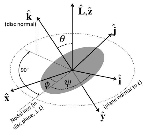
Figure 1: Euler angles used for the description of an axisymmetric grain. Figure reproduced from Ref. [24].

Between two discrete events that change its angular momentum, the grain can be considered as freely rotating. During these periods, the Euler angles change according to

$$\theta = \textrm{constant},$$ (6)

$$\dot{\phi} = \frac{L}{I_{1}},$$ (7)

$$\dot{\psi} = -\left(\frac{L}{I_{1}}-\frac{L}{I_{3}}\right)\cos\theta.$$ (8)

Electromagnetic radiation is now emitted at the four frequencies $\dot{\phi}/(2\pi),|\dot{\psi}|/(2\pi),(\dot{\phi}\pm\dot{\psi})/(2\pi)$ [24, 10]:

$$\frac{dP}{d\nu} = \frac{2\mu_{||}^{2}}{3c^{3}}\dot{\phi}^{4}\sin^{2}\theta~{}\delta\left(\nu-\frac{\dot{\phi}}{2\pi}\right)+\frac{\mu_{\bot}^{2}}{3c^{3}}\dot{\psi}^{4}\sin^{2}\theta~{}\delta\left(\nu-\frac{|\dot{\psi}|}{2\pi}\right)$$ (9)

$$+ \sum_{\pm}\frac{\mu_{\bot}^{2}}{6c^{3}}(\dot{\phi}\pm\dot{\psi})^{4}(1\pm\cos\theta)^{2}\delta\left(\nu-\frac{(\dot{\phi}\pm\dot{\psi})}{2\pi}\right).$$

2.1.3 Triaxial grain

The case of a triaxial grain is unfortunately not analytic. In that case power is radiated at a countably infinite number of frequencies. Hoang et al (2011) [11] obtained the power spectrum of a freely rotating grain numerically. They show that for a classically rotating grain, only a few modes are dominant.

2.2 Emissivity

The quantity of interest to us is the emissivity $j_{\nu}$ (with units of power per frequency interval per unit volume per steradian), which we obtain from integrating the power over grain size and shape distribution $dn_{\rm gr}/d\boldsymbol{a}$ (where $\boldsymbol{a}$ is meant to formally represent the characteristic size and three-dimensional shape of a grain), as well as the electric dipole distribution, $f(\boldsymbol{\mu}|\boldsymbol{a})$, convolved with the probability distribution for the angular momentum and rotational configuration $f(\boldsymbol{L},\boldsymbol{\varpi}|\boldsymbol{a};\boldsymbol{\mu})$. In the absence of any preferred direction, the dependence on $\boldsymbol{L}$ is in fact only through its magnitude $L$. This is the case if there are no magnetic fields and anisotropic radiation fields, or if none of them are efficient at aligning the grains. In what follows we will assume perfect isotropy of space. The emissivity is then given by

$$j_{\nu}=\frac{1}{4\pi}\int d\boldsymbol{a}\frac{dn_{\rm gr}}{d\boldsymbol{a}}\int d^{3}\boldsymbol{\mu}f(\boldsymbol{\mu}|\boldsymbol{a})\int d^{3}\boldsymbol{L}~{}d\boldsymbol{\varpi}~{}f(L,\boldsymbol{\varpi}|\boldsymbol{a},\boldsymbol{\mu})\frac{dP}{d\nu}(\nu|L,\boldsymbol{\varpi},\boldsymbol{a},\boldsymbol{\mu}).$$ (10)

Finally, we note that the actual observable is the radio intensity, given by the emissivity integrated along the line of sight,

$$I_{\nu}(\boldsymbol{\hat{n}})=\int j_{\nu}(s\boldsymbol{\hat{n}})ds.$$ (11)

At each point in space, the emissivity depends on the local environmental conditions (density, temperature, ionization degree, ambient radiation field, as well as grain abundance), as we shall see below. Therefore predicting the spinning dust spectrum along a line of sight requires modeling the ISM properties (see for example Ref. [28]). Ref. [11] evaluate the effect of turbulence on the spinning dust spectrum, and find that the effective emissivity (averaged over the probability distribution for the compression factor along the line of sight) can be shifted to larger frequencies and enhanced by several tens of percent.

We do not deal with this aspect in this review as it does not belong, per se, to the field of spinning dust theory, but rather to the larger field of ISM modeling. It is however crucial to accurately model the environmental spatial variations in order to get precise predictions.

3 Grain properties

3.1 Abundance and size distribution

The small grain abundance is determined primarily from observations of the wavelength-dependent extinction and the $3-25~{}\mu$m emission, attributed to various vibrational modes of PAHs (for a review on interstellar PAHs and their properties, see for example Tielens (2008) [26]). Observations require a few percent of the interstellar carbon to be locked in PAHs, and a significant population of very small grains (less than $\sim$ 1 nm in size) to reproduce the strength of the 3-12 $\mu$m bands, which are emitted by small grains stochastically heated to large temperatures [7]. Following DL98, Li and Draine (2001) [19] and Weingartner and Draine (2001) [27] have adopted a log-normal distribution in grain radius, starting and centered at $a_{\rm min}=a=3.5$ Å (corresponding roughly to a coronene molecule with formula C₂₄H₁₂) and variance $\sigma=0.4$ in $\log a$, and showed that such a distribution reproduced the infrared emission well. Observations tend to indicate that PAHS are less abundant in dense clouds than in the diffuse ISM.

Note that we assume that the smallest grains in the ISM are mostly PAHs, but a population of ultrasmall silicate grains is not completely ruled out by observations [20].

3.2 Shapes

PAHs may take a variety of shapes, from disk-like to nearly linear. They are not necessarily planar: for example if one of the hexagonal carbon rings is replaced by a pentagonal ring, they are bent and become three-dimensional. Above a certain size, PAHs may form irregular clusters, and eventually, large three-dimensional grains.

The exact distribution of shapes is largely unknown. The lowest-frequency IR emission bands in principle carry information about the individual grains, and seem to indicate that PAHs may be dominated by a few well-defined molecular structures, although not conclusively [26].

The smallest grains dominate the spinning dust spectrum (they can be spun up to larger frequencies and hence emit more power). It is commonly assumed that these grains are nearly planar up to a spherical-equivalent radius $a=6$ Å, corresponding to 100 carbon atoms. The peak of the spinning dust spectrum is not very sensitive to the exact cutoff between planar and spherical grains.

3.3 Permanent dipole moments

In principle a consistent prescription should be given for small grains, that gives the precise nature of the grain, hence its shape (or rotational constants) and permanent electric dipole moment, which can be computed quantum-mechanically for small enough molecules. Such computations were carried out by Hudgins, Bauschlicher and Allamandola (2005) [13] for nitrogen-substituted PAHs. They found typical permanent dipole moments of a few Debyes, depending on the precise position of the substituted nitrogen atom.

Eventually, observations will hopefully allow for a more precise determination of the population of PAHs and their properties. We are currently far from having a definite handle on such refined properties of small grains, and an empirical distribution of dipole moments is required. Following DL98, more recent models assume a three-dimensional gaussian distribution of dipole moments, with variance

$$\langle\boldsymbol{\mu}^{2}\rangle=N_{\rm at}\beta^{2}+(\epsilon aeZ)^{2},$$ (12)

where $\beta\approx 0.4$ Debye and $\epsilon\approx 0.01$. The first term, largely dominant, accounts for the permanent dipole moment and the second term accounts for charge displacement in ionized grains. We repeat that this distribution is largely ad hoc and may be far from reflecting reality, except (hopefully) for the characteristic permanent dipole moment.

4 Rotational configuration

4.1 Fast vibration-rotation energy transfer

In principle one should solve for the distribution of angular momentum and rotational configuration $f(L,\boldsymbol{\varpi})$ at once. Indeed, a priori, the same processes that change the angular momentum may also change the relative orientation of the grain at a similar rate. Grains can exchange angular momentum with several “baths”, all characterized by different characteristic “temperatures”, and the resulting overall distribution function cannot easily be factored into a pure angular momentum part and a pure rotational configuration part (one can always formally write the factorization, $f(L,\boldsymbol{\varpi})=f(L)f(\boldsymbol{\varpi}|L)$, but one cannot in principle compute the two factors independently).

The situation is much simplified if one single process is very efficient at changing the rotational configuration, on timescales much shorter than the overall timescale to change the angular momentum. If this process is characterized by an equilibrium temperature $T_{\boldsymbol{\varpi}}$, then one can indeed compute the probability distribution $f(\boldsymbol{\varpi}|L)$ independently:

$$f(\boldsymbol{\varpi}|L)\propto\exp\left[-\frac{E_{\rm rot}(L,\boldsymbol{\varpi})}{kT_{\boldsymbol{\varpi}}}\right],$$ (13)

where the rotational energy is most easily written using the projections of the angular momentum on the grain’s principal axes with principal moments of inertia $I_{i}$,

$$E_{\rm rot}(L,\boldsymbol{\varpi})=\sum_{i}\frac{L_{i}^{2}}{2I_{i}}=L^{2}\sum_{i}\frac{l_{i}^{2}}{2I_{i}},$$ (14)

where we have defined $l_{i}\equiv L_{i}/L$, the normalized projection of the angular momentum along the axis $i$. One can formally identify $\boldsymbol{\varpi}\leftrightarrow\{l_{i}\}$ (at least in some time-averaged sense), and Eq. (13) then uniquely determines the probability distribution for the rotational configuration, given a value for the total angular momentum $L$. The angular momentum distribution $f(L)$ can then be obtained from transition rates averaged over the rotational configuration with the known distribution $f(\boldsymbol{\varpi}|L)$.

Luckily Nature does provide us with such an efficient process to change $\boldsymbol{\varpi}$ at constant $L$: internal vibrational-rotational energy transfer (IVRET) (see for example [22, 16, 25] and [24, 11] for application to spinning dust modeling). The first detailed studies of how internal relaxation may affect grain alignment were carried in Refs. [15, 17].

Following the absorption of an ultraviolet (UV) photon, small grains get heated up to large vibrational temperatures $T_{\rm vib}$ (the notion of temperature is not well defined for the smallest grains, so we mean temperature as a characteristic energy per degree of freedom). IVRET leads to a rapid energy exchange between vibrational and rotational degrees of freedom, at constant angular momentum, so that during a thermal spike, the distribution $f(\boldsymbol{\varpi}|L)$ is given by Eq. (13) with $T_{\boldsymbol{\varpi}}=T_{\rm vib}$. As the grain cools down by emitting infrared photons, its vibrational temperature decreases, until the grain reaches its fundamental vibrational mode, with typical energy $E_{0}/k\sim 100$ K for the smallest grains. IVRET is only active as long as the density of vibrational states is large enough that there exist transitions at frequencies near the rotation frequency. Therefore energy exchange freezes at a characteristic temperature $T_{\boldsymbol{\varpi}}=T_{\rm fr}>E_{0}/k$, probably of at least a couple hundred Kelvins, and this temperature characterizes the final rotational configuration following a thermal spike. For this distribution to remain valid at all times, it is necessary that the rate of absorption of UV photons is larger than the rate of change of angular momentum. This is indeed the case in diffuse environments (see Table 1 of Ref. [24]), where absorption of UV photons is a few times faster than angular momentum changes; this difference of timescales gets more pronounced as the ambient radiation field increases. In dense and under-illuminated clouds, however, the rate of absorption of photons is not large enough to maintain the distribution (13), and the rotational configuration needs in principle to be computed from the full $f(L,\boldsymbol{\varpi})$.

Let us now discuss the implications of Eq. (13). The angular momentum itself is has a characteristic value $L_{\rm peak}$, and therefore the rotational energy is of order $E_{\rm rot}\sim L_{\rm peak}^{2}/I\equiv kT_{L}$. If $T_{\boldsymbol{\varpi}}\ll T_{L}$, the most probable rotational configuration will be the one minimizing the energy, i.e. where the grain rotates about its axis of greatest inertia. In the opposite case where $T_{\boldsymbol{\varpi}}\gg T_{L}$, all rotational configurations become equiprobable (of course when converting to actual angles one needs to be careful of using the appropriate phase-space volume $d\boldsymbol{\varpi}$).

For example, an axisymmetric oblate grain with $I_{3}>I_{2}=I_{1}$ has a rotational energy

$$E_{\rm rot}(L,\theta)=\frac{L^{2}}{2I_{1}}\left[1-\left(1-\frac{I_{1}}{I_{3}}\right)\cos^{2}\theta\right],$$ (15)

where $\theta$ is the angle between $\boldsymbol{L}$ and the axis of greatest inertia. If $T_{\boldsymbol{\varpi}}\ll T_{L}$, the most probable configurations are $\theta=0$ or $\pi$. In the case where $T_{\boldsymbol{\varpi}}\gg T_{L}$, we obtain that $f(\theta|L)\propto\sin\theta$ (here we used $d\boldsymbol{\varpi}=d\phi\sin\theta d\theta$ in the usual spherical polar coordinates).

SpDust only allows for the two limiting regimes $T_{\boldsymbol{\varpi}}\rightarrow 0$ and $T_{\boldsymbol{\varpi}}\rightarrow\infty$, bracketing the range of possibilities. The authors of Ref. [11] explore the effect of continuously varying $T_{\boldsymbol{\varpi}}$, interpolating continuously between the two extreme regimes. In general there will be a different temperature $T_{\boldsymbol{\varpi}}$ for each grain size and depending on the environment, but the precise modeling of this parameter has not been addressed in the literature yet. In what follows we shall only discuss the two limiting regimes.

4.2 Implication for the emitted power at fixed angular momentum

The last integral in Eq. (10) can be rewritten as

$$\int d^{3}\boldsymbol{L}d\boldsymbol{\varpi}f(L,\boldsymbol{\varpi})\frac{dP}{d\nu}(L,\boldsymbol{\varpi})=\int d^{3}\boldsymbol{L}f(L)\Big{\langle}\frac{dP}{d\nu}\Big{\rangle}(L),$$ (16)

where the power averaged over the rotational configuration is

$$\Big{\langle}\frac{dP}{d\nu}\Big{\rangle}(L)\equiv\int d\boldsymbol{\varpi}f(\boldsymbol{\varpi}|L)\frac{dP}{d\nu}(L,\boldsymbol{\varpi}).$$ (17)

In the case of a grain rotating about its axis of greatest inertia $I_{3}$, the averaged power collapses to

$$\Big{\langle}\frac{dP}{d\nu}\Big{\rangle}=\frac{2}{3c^{3}}(2\pi\nu)^{4}\mu_{\bot}^{2}\delta(\nu-L/(2\pi I_{3})),\ \ \ \ T_{\boldsymbol{\varpi}}\rightarrow 0,$$ (18)

which is identical to the case of a spherical grain. If we now consider an oblate axisymmetric grain with $T_{\boldsymbol{\varpi}}\rightarrow\infty$, we obtain, using the results of Section 2.1.2, and averaging over isotropically distributed nutation angles $\theta$,

$$\Big{\langle}\frac{dP}{d\nu}\Big{\rangle} = \frac{4\mu_{||}^{2}}{9c^{3}}(2\pi\nu_{1})^{4}\delta(\nu-\nu_{1})+\frac{\mu_{\bot}^{2}}{3c^{3}}(2\pi\nu)^{4}\left[1-\left(\frac{\nu}{\nu_{13}}\right)^{2}\right]\frac{\boldsymbol{1}_{\nu<\nu_{13}}}{\nu_{13}}$$ (19)

$$+ \frac{\mu_{\bot}^{2}}{3c^{3}}(2\pi\nu)^{4}\left(\frac{\nu_{1}+\nu_{13}-\nu}{\nu_{13}}\right)^{2}\frac{\boldsymbol{1}_{\nu_{3}<\nu<\nu_{1}+\nu_{13}}}{2\nu_{13}},\ \ \ \ T_{\boldsymbol{\varpi}}\rightarrow\infty,$$

where the function $\boldsymbol{1}$ is unity where its subscript is valid and zero elsewhere, and we have defined the two frequencies

$$\nu_{1} \equiv \frac{L}{2\pi I_{1}},$$ (20)

$$\nu_{13} \equiv \frac{L}{2\pi I_{1}}-\frac{L}{2\pi I_{3}}.$$ (21)

In the case of a planar grain with with $I_{3}=2I_{1}$ and $\nu_{1}=2\nu_{3}=2\nu_{13}$, the power radiated by a wobbling grain is emitted at characteristic frequencies about twice as large as in the case of a grain rotating primarily about its axis of greatest inertia. The integrated power is, in the former case (and assuming $\nu_{3}=\nu_{13}$)

$$P(T_{\boldsymbol{\varpi}}\rightarrow\infty)=\frac{4\mu_{||}^{2}}{9c^{3}}(2\pi\nu_{1})^{4}+10\frac{\mu_{\bot}^{2}}{3c^{3}}(2\pi\nu_{3})^{4},$$ (22)

which is about 10 times larger, at equal angular momentum, than the power radiated by a grain rotating mostly about its axis of greatest inertia, if $\mu_{\bot}^{2}=2\mu_{||}^{2}$.

One must not forget, however, that the angular momentum distribution itself depends upon the rotational configuration $f(\boldsymbol{\varpi}|L)$, since one must use this distribution to average transition rates. We shall see in the next section that the effect of randomized rotational configuration is to lower the characteristic angular momentum $L$.

5 Angular momentum distribution

To determine the angular momentum distribution, we need to evaluate the differential transition rates $\Gamma(L\rightarrow L^{\prime})$ between different values of the angular momentum magnitude, defined such that $\Gamma(L\rightarrow L^{\prime})\Delta L^{\prime}$ is the rate of transition from an initial angular momentum $L$ to a final angular momentum in the interval $[L^{\prime},L^{\prime}+\Delta L^{\prime}]$. These rates are averaged over the rotational configuration for $\boldsymbol{\varpi}$ discussed above. The steady-state distribution function $f(L)$ should then in principle be obtained from the integral master equation,

$$\frac{\partial\tilde{f}(L)}{\partial t}=\int\left[\tilde{f}(L^{\prime})\Gamma(L^{\prime}\rightarrow L)-\tilde{f}(L)\Gamma(L\rightarrow L^{\prime})\right]dL^{\prime}=0,\ \ \textrm{for all}\ L,$$ (23)

where we have defined $\tilde{f}(L)\equiv 4\pi L^{2}f(L)$ so that $\tilde{f}(L)$ is the distribution function for the magnitude of $\boldsymbol{L}$ (whereas $f(\boldsymbol{L})=f(L)$ is the distribution function for the vector angular momentum, even if it only depends on its magnitude due to isotropy). This equation is, clearly, rather cumbersome to solve and below we present a simpler (if approximate) method of solution, based on the Fokker-Planck equation. Section 5.1 provides a formal introduction to the problem, and actual physical mechanisms are discussed in Section 5.2.

5.1 The Fokker-Planck equation

5.1.1 Derivation

In general transition rates are not significant for arbitrarily large values of $\Delta L\equiv L^{\prime}-L$: there always exists some characteristic $\Delta L_{0}$ such that $\Gamma(L\rightarrow L+\Delta L)$ decreases rapidly for $|\Delta L|\gtrsim\Delta L_{0}$. An important simplification can be made if the scale $\Delta L_{0}$ is much smaller than the characteristic scale over which both the distribution function varies and the rates themselves vary – the distribution function being unknown a priori, the validity this assumption has in principle to be checked a posteriori. If this is the case, we may expand the first term in the integral of Eq. (23), setting $L^{\prime}=L+\Delta L$:

$$\tilde{f}(L+\Delta L)\Gamma(L+\Delta L\rightarrow L) \approx \tilde{f}(L)\Gamma(L\rightarrow L-\Delta L)+\Delta L\frac{\partial}{\partial L}\left[\tilde{f}(L)\Gamma(L\rightarrow L-\Delta L)\right]$$ (24)

$$+ \frac{1}{2}(\Delta L)^{2}\frac{\partial^{2}}{\partial L^{2}}\left[\tilde{f}(L)\Gamma(L\rightarrow L-\Delta L)\right].$$

Plugging this expansion back into Eq. (23), we see that the term linear in $\tilde{f}(L)$ cancels out with the second term of the integral (the integrand being an odd function of $\Delta L$). Recalling that $\tilde{f}(L)=4\pi L^{2}f(L)$, we finally obtain

$$4\pi L^{2}\frac{\partial f(L)}{\partial t}=-\frac{\partial}{\partial L}\left[\frac{d\langle\Delta L\rangle}{dt}4\pi L^{2}f(L)\right]+\frac{1}{2}\frac{\partial^{2}}{\partial L^{2}}\left[\frac{d\langle(\Delta L)^{2}\rangle}{dt}4\pi L^{2}f(L)\right]=0,$$ (25)

where we have defined the rate of angular momentum drift (the opposite of which is the rate of angular momentum dissipation or damping),

$$\frac{d\langle\Delta L\rangle}{dt}\equiv\int\Delta L~{}\Gamma(L\rightarrow L+\Delta L)d(\Delta L),$$ (26)

and the rate of angular momentum diffusion (also termed fluctuation or excitation),

$$\frac{d\langle(\Delta L)^{2}\rangle}{dt}\equiv\int(\Delta L)^{2}\Gamma(L\rightarrow L+\Delta L)d(\Delta L).$$ (27)

Equation (25) is known as the Fokker-Planck equation and has a broad range of applications in physics (see for example Chapter 6 of the book [3] by Blandford and Thorne). In the context of grain rotation, this approach was used in Refs. [8, 14, 2, 24], and is the basic equation solved in SpDust. Solving this equation is much simpler than solving the full master equation, and it may even have a simple analytic solution if the excitation and damping rates are simple enough.

5.1.2 General form of the rates and solution

General processes besides electric dipole radiation damping.

Most processes through which grains may change angular momentum (except for electric dipole radiation itself, to which we shall come back later on) are characterized by a damping timescale $\tau$ such that

$$\frac{d\langle\Delta\boldsymbol{L}\rangle}{dt}=-\frac{\boldsymbol{L}}{\tau}$$ (28)

and have an isotropic and constant diffusion rate of the form

$$\frac{d\langle\Delta L_{i}\Delta L_{j}\rangle}{dt}=\frac{1}{3}\frac{\sigma_{L}^{2}}{\tau}\delta_{ij}.$$ (29)

Taylor-expanding $\Delta L$ to second order in $\Delta\boldsymbol{L}$, we obtain

$$\Delta L=|\boldsymbol{L}+\Delta\boldsymbol{L}|-L\approx\Delta\boldsymbol{L}\cdot\boldsymbol{\hat{L}}+\frac{(\Delta\boldsymbol{L})^{2}-(\Delta\boldsymbol{L}\cdot\boldsymbol{\hat{L}})^{2}}{2L}.$$ (30)

The excitation and damping rates for the magnitude of the angular momentum are therefore

$$\frac{d\langle\Delta L\rangle}{dt} = \frac{\sigma_{L}^{2}/3-L^{2}}{L\tau},$$ (31)

$$\frac{d\langle(\Delta L)^{2}\rangle}{dt} = \frac{\sigma_{L}^{2}}{3\tau}.$$ (32)

The form of these coefficients stems from the fact that only longitudinal excitation generates a true diffusion in the magnitude of $\boldsymbol{L}$, whereas excitations perpendicular to $\boldsymbol{L}$ lead to a systematic increase of the magnitude of the angular momentum, and hence appear as a positive drift rate in Eq. (31).

If only one single process was interacting with the grains, their steady-state distribution would then be the Maxwellian with three-dimensional variance $\langle L^{2}\rangle=\frac{1}{2}\sigma_{L}^{2}$,

$$f(L)\propto\exp\left[-\frac{3L^{2}}{\sigma_{L}^{2}}\right],$$ (33)

as can be seen from inserting the rates (31) and (32) into the Fokker-Planck equation (25).

Often, however, there is not a single process that dominates both excitation and damping. Since transition rates add up linearly for independent processes, so do excitation and damping rates. If all rates are of the form (28), (29), then the final distribution is still Maxwellian, with a variance weighted by the characteristic rates of the various processes indexed by $\alpha$:

$$f(L)\propto\exp\left[-\frac{3L^{2}}{\sigma_{L}^{2}}\right],\ \ \ \ \sigma_{L}^{2}\equiv\frac{\sum_{\alpha}\tau_{\alpha}^{-1}\sigma_{L,\alpha}^{2}}{\tau^{-1}},\ \ \ \ \tau^{-1}\equiv\sum_{\alpha}\tau_{\alpha}^{-1}.$$ (34)

Damping through electric dipole radiation.

One process behaves differently from Eqs. (28), (29): the damping of angular momentum through electric dipole radiation itself. Since the rotational energy is proportional to $L^{2}$ and the radiated power is proportional to $L^{4}$, the rate of angular momentum damping scales as $L^{3}$. We may write it in the form

$$\frac{d\langle\Delta\boldsymbol{L}\rangle}{dt}|_{\rm ed}=-\frac{L^{2}\boldsymbol{L}}{\sigma_{L}^{2}\tau_{\rm ed}},$$ (35)

where we may take the variance $\sigma_{L}^{2}$ to be that given by Eq. (34). This defines $\tau_{\rm ed}$ as the characteristic timescale to damp an angular momentum of order $\sigma_{L}$ through electric dipole radiation (note that this definition of $\tau_{\rm ed}$ is different from the ones adopted in Refs. [6, 2], where $\sigma_{L}^{2}=3IkT_{\rm gas}$ was specifically used in Eq. (35) to define $\tau_{\rm ed}$). Every damping process has in general an associated excitation process, and vice versa. In the case of electric dipole radiation, the associated fluctuation in angular momentum is due to absorption of and decays stimulated by microwave photons (dominated by Cosmic Microwave Background (CMB) photons in the diffuse ISM). To our knowledge this process was only considered in Ref. [1] and we shall get back to it in the next section.

Accounting for the damping only for now and including this additional damping into the Fokker-Planck equation, we obtain the solution

$$f(L)\propto\exp\left[-3\frac{L^{2}}{\sigma_{L}^{2}}-\frac{3}{2}\frac{\tau}{\tau_{\rm ed}}\frac{L^{4}}{\sigma_{L}^{4}}\right].$$ (36)

The most likely angular momentum for this distribution is such that the net drift rate vanishes,

$$L_{\rm peak}^{2}=\frac{\sigma_{L}^{2}}{3}\frac{2}{1+\sqrt{1+\frac{4}{3}\frac{\tau}{\tau_{\rm ed}}}}.$$ (37)

For $\tau_{\rm ed}\ll\tau$, which is often the case for the smallest grains, the most likely angular momentum results from equilibrium between damping through electric dipole radiation and excitations through other mechanisms, and is approximately

$$L_{\rm peak}^{2}\approx\sqrt{\frac{\tau_{\rm ed}}{\tau}}\sigma_{L}^{2},\ \ \tau_{\rm ed}\ll\tau.$$ (38)

In that case, the characteristic damping time at the peak is $\tau_{\rm rot}=\sqrt{\tau\tau_{\rm ed}}$. In general, one can define a characteristic damping time as

$$\tau_{\rm rot}\approx\min[\tau,\sqrt{\tau\tau_{\rm ed}}].$$ (39)

We can rewrite the peak angular momentum in terms of $\tau_{\rm rot}$ as

$$L_{\rm peak}^{2}\sim\frac{\tau_{\rm rot}}{\tau}\sigma_{L}^{2}.$$ (40)

5.1.3 Limitation of the Fokker-Planck approach: impulsive torques

The Fokker-Planck equation is a diffusion equation, and its validity is limited to processes that change the angular momentum by small increments. In this section we formally discuss in which cases it may break down.

Let us now consider some stochastic interaction process $\alpha$ (in practice, collisions with passing ions [10]) with rate $\tau_{\rm coll}^{-1}$, such that the characteristic angular momentum exchanged with a grain at each interaction has variance

$$\langle\Delta L_{i}\Delta L_{j}\rangle_{\alpha}=\frac{\tau_{\rm coll}}{\tau_{\alpha}}\frac{\sigma_{L,\alpha}^{2}}{3}\delta_{ij}.$$ (41)

The diffusion rate for such an interaction is indeed, formally equal to that of Eq. (29). However, this process can only be considered as diffusive if $\langle(\Delta L)^{2}\rangle_{\alpha}\ll L_{\rm peak}^{2}$. This translates to the condition

$$\tau_{\rm coll}\ll\tau_{\rm rot}~{}\frac{\tau^{-1}\sigma_{L}^{2}}{\tau_{\alpha}^{-1}\sigma_{L,\alpha}^{2}}.$$ (42)

If the process $\alpha$ is the dominant excitation mechanism, $\tau^{-1}\sigma_{L}^{2}=\tau_{\alpha}^{-1}\sigma_{L,\alpha}^{2}$ and the condition for the validity of the diffusion approximation is that $\tau_{\rm coll}\ll\tau_{\rm rot}$, the characteristic time to change the angular momentum.

The issue of impulsive torques was addressed by Hoang et al [10]. Instead of solving a Fokker-Planck equation, Hoang et al start with the Langevin equation, of the form

$$dL=\frac{d\langle\Delta L\rangle}{dt}dt+\sqrt{\frac{d\langle(\Delta L)^{2}\rangle}{dt}}dq,$$ (43)

where $dq$ is a random variable with variance $\langle(dq)^{2}\rangle=dt$. They then solve it numerically to obtain $L(t_{i})$ at a set of discret timesteps $t_{i}$. The distribution function $f(L)$ is then obtained from the histogram of values of $L_{i}$ after a long enough evolution. In the form (43), the Langevin equation is exactly equivalent to the Fokker-Planck equation, in the sense that it assumes infinitesimal torques. However, it is simple to generalize this treatment to include impulsive toques. First, one draws the interval between two collisions from the Poisson distribution with mean $\tau_{\rm coll}$. Second, an angular momentum $\Delta\boldsymbol{L}$, is drawn from an isotropic distribution with variance $\langle(\Delta L)^{2}_{\rm coll}\rangle$. This method allows to include random impulsive torques in addition to the quasi-continuous torques. We defer the discussion of Hoang et al’s results to Section 5.4.

5.2 Excitation and damping rates for various mechanisms

In this section we describe the principal mechanisms that excite and damp the grains’ rotation. Since the detailed calculations are already worked out in various papers [6, 23, 2, 24], here we limit ourselves to giving a semi-qualitative description of each process and order of magnitude estimates for the relevant rates. Since the smallest grains are producing the peak of the spinning dust spectrum, all numerical evaluations are normalized to the characteristic radius of coronene, $a\approx 3.5$ Å.

5.2.1 Collisions

Collisional interactions of grains with gas atoms, molecules or ions is perhaps the most intuitive of angular momentum transfer processes, even though the microphysical details could be very complex (see for example the discussion in Section 4.2 of Ref. [23]). Impactors with density $n_{\rm imp}$ reach the grain with a rate

$$\tau_{\rm coll}^{-1}\approx n_{\rm imp}\pi b_{\rm max}^{2}\overline{v}_{\rm in},$$ (44)

where $\pi b_{\rm max}^{2}$ is the effective collisional cross-section ($b_{\rm max}$ being the maximal impact parameter for which a collision occurs) and $\overline{v}_{\rm in}$ is the characteristic velocity of the impactors at infinity. As they impact the grain, they stick to its surface, providing there are available adsorption sites. The random angular momentum transferred to the grain has variance

$$\langle(\Delta L)^{2}\rangle_{\rm in}\sim(m_{\rm imp}b_{\rm max}\overline{v}_{\rm in})^{2},$$ (45)

where $m_{\rm imp}$ is the mass of the impactor.

The attached impactors are ejected from the grain’s surface following the absorption of UV photons that heat up small grains to large temperatures (this is the process of photoevaporation). Because ions are in general more electronegative than large molecules, they leave the grain surface as neutral species. Here again, they give a random recoil to the grain, leading to

$$\langle(\Delta L)^{2}\rangle_{\rm out}\sim(m_{\rm imp}a\overline{v}_{\rm out})^{2},$$ (46)

where $\overline{v}_{\rm out}$ is the characteristic velocity of ejection, related to the dust grain temperature $T_{\rm vib}$ following thermal spikes by $m_{\rm imp}v_{\rm out}^{2}\sim kT_{\rm vib}$.

In addition to a random component, ejected particles systematically decrease the angular momentum of the grain: if their ejection velocity is random in the rotating grain’s frame, they carry on average an angular momentum

$$\Delta L_{\rm out}=m_{\rm imp}a^{2}\omega\sim\frac{m_{\rm imp}a^{2}}{I}L\sim\frac{m_{\rm imp}}{m_{\rm grain}}L,$$ (47)

where $\omega$ is the rotation rate of the grain and $I\sim m_{\rm grain}a^{2}$ is its characteristic moment of inertia. In steady-state, the rate of ejections equals the rate of collisions and therefore

$$\frac{d\langle\Delta L\rangle}{dt}\sim-\tau_{\rm coll}^{-1}\frac{m_{\rm imp}}{m_{\rm grain}}L.$$ (48)

From this expression we see that the characteristic timescale for damping the angular momentum through ejection of colliding gas particles is

$$\tau\sim\frac{m_{\rm grain}}{m_{\rm imp}}\tau_{\rm coll}.$$ (49)

Using the definition (32), we see that the characteristic variance in angular momentum that would stem from collisions alone is

$$\sigma_{L}^{2}\sim\frac{\tau}{\tau_{\rm coll}}\langle(\Delta L)^{2}\rangle\sim\frac{I}{m_{\rm imp}a^{2}}\left[(m_{\rm imp}b_{\rm max}\overline{v}_{\rm in})^{2}+(m_{\rm imp}a\overline{v}_{\rm out})^{2}\right]\sim I\left[\frac{b_{\rm max}^{2}}{a^{2}}kT_{\rm in}+kT_{\rm out}\right].$$ (50)

We see that collisions tend to drive the angular momentum distribution to a thermal distribution with temperature

$$T_{L,\rm coll}\approx\frac{1}{2}\left[\frac{b_{\rm max}^{2}}{a^{2}}T_{\rm in}+T_{\rm out}\right].$$ (51)

The maximum impact parameter (or effective cross-section) for incoming particles depends upon the charge state of the grain and impactor. It can easily be determined at an order-of magnitude for a spherically symmetric interaction potential $V(r)$. Requiring energy and angular momentum conservation, we find

$$\left(\frac{b_{\rm max}}{a}\right)^{2}\sim 1-\frac{V(a)}{E_{\rm in}}\sim 1-\frac{V(a)}{kT_{\rm in}}.$$ (52)

In the case of a repulsive interaction $V>0$, this should be understood as $b_{\rm max}\approx a$ if $V(a)\ll kT_{\rm in}$ and 0 in the opposite case.

$\bullet$ For neutral impactors and neutral grains, $b_{\rm max}=a$.

$\bullet$ For neutral impactors and charged grains (with charge $Z_{g}e$), the collisional cross-section can be determined from equating the kinetic energy of the incoming particle to the potential energy of the attractive induced-dipole interaction,

$$V(r)=-\frac{1}{2}\alpha\frac{Z_{g}^{2}e^{2}}{r^{4}},$$ (53)

where $\alpha$ is the polarizability of the impactor. Typically, $\alpha\approx 1$ ų so the focusing factor $(b_{\rm max}/a)^{2}$ is of order $\sim 1+(T/10^{3}$ K)^-1 for $a\approx 3.5$ Å. This potential must also be accounted for when evaluating the escape probability of neutral particles ejected from ionized grains.

$\bullet$ For positively charged impacting ions, the dominant interaction is the attractive Coulomb attraction with negatively charged grains,

$$V(r)=-\frac{|Z_{i}Z_{g}|e^{2}}{r},$$ (54)

corresponding to a large focusing factor

$$\left(\frac{b_{\rm max}}{a}\right)^{2}\approx\frac{|Z_{i}Z_{g}|e^{2}}{akT}\approx 50\left(\frac{a}{3.5\textrm{ \AA}}\right)^{-1}\left(\frac{T}{10^{3}\textrm{K}}\right)^{-1}.$$ (55)

Therefore we see that collisions with ions may overcome collisions with neutrals even for relatively small ionization degrees.

5.2.2 Plasma excitation and drag

Ions can exchange angular momentum with the grains at a distance, without necessarily colliding with them, by exerting a torque on their permanent electric dipole moment,

$$\frac{d\boldsymbol{L}}{dt}=\boldsymbol{\mu}\times\boldsymbol{E}\sim\mu\frac{Z_{i}e}{r^{2}}.$$ (56)

The characteristic interaction timescale being $\Delta t\sim b/v$, the variance of the angular momentum change for each interaction event is

$$\langle(\Delta L)^{2}\rangle\sim\left(\frac{\mu Z_{i}e}{bv}\right)^{2}.$$ (57)

Integrating over impact parameters $b$ and velocities of ions $v$, one obtains the rate of angular momentum diffusion

$$\frac{\langle(\Delta L)^{2}\rangle}{dt}\sim n_{i}(\mu Z_{i}e)^{2}\sqrt{\frac{m_{i}}{kT}}\ln\Lambda,$$ (58)

where the order-unity Coulomb logarithm $\ln\Lambda=\ln(b_{\rm hi}/b_{\rm lo})$ appears because of the logarithmic divergence of the integral over impact parameters. In practice the lower cutoff must be set to the maximal impact parameter leading to a collision (denoted $b_{\rm max}$ in the previous section), in order not to double-count the angular momentum transfer in collisions. The upper cutoff comes from the fact that when the interaction timescale $b/v$ is much larger than the rotation timescale $\omega^{-1}$, the torque along the angular momentum vector averages out to zero [2].

To obtain the damping rate from first principles would require accurate evaluations of the back-reaction of the grain on the ions’ trajectories, leading to a small asymmetry between trajectories increasing the magnitude of $\boldsymbol{L}$ and those decreasing it. However, a powerful theorem, the fluctuation-dissipation theorem [3, 4], allows us to very simply evaluate the dissipation rate from the fluctuation rate if the interaction is with a thermal bath. Put simply, excitation and damping must balance in such a way that, if only the thermal process considered was at play, the resulting distribution would also be thermal, of the form $f(L)\propto\exp[-E(L)/kT]$ with the same temperature $T$ as the bath.

In the case of a grain rotating about its axis of greatest inertia, and using the notation of Section 5.1.2, the damping timescale for plasma drag $\tau_{p}$ must therefore be such that

$$3\tau_{p}\frac{\langle(\Delta L)^{2}\rangle}{dt}=\sigma_{L,p}^{2}=6IkT_{\rm gas}.$$ (59)

The case of a wobbling grain is a little more complex, since the temperature for the rotational configuration is set by the internal relaxation process and is in general different from the gas temperature. However, one can use a closely related principle, that of detailed balance, to compute the proper damping rate given the tensorial excitation rate. Details can be found in Ref. [24].

5.2.3 Emission of infrared photons

Every time a small dust grain absorbs a UV photon, it gets into a highly excited vibrational state from which it decays by emitting a cascade of infrared (IR) photons, typically about a hundred per absorbed UV photon. Each one of the emitted IR photons carries one quantum of angular momentum, so its angular momentum squared is $L_{\gamma}^{2}=2\hbar^{2}$. If photons are emitted isotropically with a energy flux $F_{\nu}$, the rate of diffusion of angular momentum is then

$$\frac{d\langle(\Delta L)^{2}\rangle}{dt}=\frac{1}{3}2\hbar^{2}\int d\nu\frac{F_{\nu}}{h\nu}.$$ (60)

A ro-vibrational transition from the excited state $(v,J)$ [$v$ denoting the vibrational configuration and $J$ the rotational quantum number] to an other state $(v^{\prime},J+\Delta J)$ has a transition frequency

$$\nu=\nu_{0}-\frac{\omega}{2\pi}\Delta J,$$ (61)

where $\nu_{0}$ is the transition frequency for $(v,J)\rightarrow(v^{\prime},J)$ and $\omega=\hbar J/I$ is the angular rotation frequency. Quantum-mechanical transition rates are proportional to the transition frequency cubed. Summing over the three allowed transitions $\Delta J=0,\pm 1$ (and assuming they have nearly the same matrix elements), the net rate of angular momentum drift relates to the rate of photon emission $\dot{N}_{\gamma}$ through

$$\dot{J}=-3\frac{\omega}{2\pi\nu_{0}}\frac{2}{3}\dot{N}_{\gamma},$$ (62)

which implies, in the case of a grain rotating about its axis of greatest inertia,

$$\frac{d\langle\boldsymbol{L}\rangle}{dt}=-2\frac{\boldsymbol{L}}{(2\pi)^{2}I}\int d\nu\frac{F_{\nu}}{\nu^{2}}.$$ (63)

A classical calculation can be found in Refs. [6] (with missing factors of two for both damping and excitation rates), [2] (with a missing factor of two for the excitation rate) and [24]. A fully rigorous quantum-mechanical treatment can be found in Refs. [2, 1, 23, 29]. They are perfectly equivalent since ISM grains are classical rotators.

The main difficulty in correctly evaluating Eqs. (60) and (63) is that one must be able to compute the infrared spectrum with high accuracy, especially at long wavelengths (where it is not well constrained by observations).

5.2.4 Electric dipole radiation and absorption of CMB photons

Damping rate

A grain emitting electric dipole radiation also radiates away angular momentum. Classically, the radiation reaction torque is given by

$$\frac{d\langle\Delta\boldsymbol{L}\rangle}{dt}|_{\rm ed}=-\frac{2}{3c^{3}}\langle\dot{\boldsymbol{\mu}}\times\ddot{\boldsymbol{\mu}}\rangle,$$ (64)

where the averaging is over the quasi-periodic rotation of the grain. For a grain rotating about its axis of greatest inertia, the result is

$$\frac{d\langle\Delta\boldsymbol{L}\rangle}{dt}|_{\rm ed}=-\frac{2\mu_{\bot}^{2}}{3c^{3}}\left(\frac{L}{I_{3}}\right)^{3}\boldsymbol{\hat{L}},\ \ \ T_{\boldsymbol{\varpi}}\rightarrow 0.$$ (65)

In the case of a wobbling disk-like grain with completely randomized nutation state, the corresponding damping rate is (assuming $I_{3}=2I_{1}$ for simplicity) [24]:

$$\frac{d\langle\Delta\boldsymbol{L}\rangle}{dt}|_{\rm ed}=-\left[\frac{82\mu_{\bot}^{2}}{45c^{3}}+\frac{32\mu_{||}^{2}}{9c^{3}}\right]\left(\frac{L}{I_{3}}\right)^{3}\boldsymbol{\hat{L}},\ \ \ T_{\boldsymbol{\varpi}}\rightarrow\infty.$$ (66)

The characteristic timescale to damp an angular momentum $L=\sigma_{L}$ [defined in Eq. (35)] is therefore such that

$$\tau_{\rm ed}^{-1} = \frac{2\mu_{\bot}^{2}}{3c^{3}}\frac{\sigma_{L}^{2}}{I_{3}^{3}},\ \ \ \ \ \ \ \ \ \ \ \ \ \ \ \ \ \ \ T_{\boldsymbol{\varpi}}\rightarrow 0,$$ (67)

$$= \left[\frac{82\mu_{\bot}^{2}}{45c^{3}}+\frac{32\mu_{||}^{2}}{9c^{3}}\right]\frac{\sigma_{L}^{2}}{I_{3}^{3}},\ \ \ T_{\boldsymbol{\varpi}}\rightarrow\infty.$$ (68)

We see that the electric dipole radiation damping timescale is typically about 5 times shorter if the grain is wobbling than when it is rotating primarily about its axis of greatest inertia.

Excitation rate

The associated excitation mechanism comes from the absorption of CMB photons [1]. For simplicity, here we only consider the case of a grain rotating abouts its axis of greatest inertia.

Quantum mechanically, the damping of the angular momentum is due to spontaneous decays $J\rightarrow J-1$, with rate $A_{J,J-1}$, so we may rewrite

$$\frac{d\langle\Delta\boldsymbol{L}\rangle}{dt}|_{\rm ed}=-\hbar A_{J,J-1}\boldsymbol{\hat{L}}.$$ (69)

In addition to these spontaneous decays, stimulated decays take place, as well as absorptions of CMB photons. For large $J$, the net angular momentum change due to these transition nearly cancel out (so the drift is essentially due to spontaneous decays). However, the rate of excitation parallel to the angular momentum axis is (in the limit that $J\gg 1$),

$$\frac{d\langle(\Delta\boldsymbol{L}_{||})^{2}\rangle}{dt}|_{\rm ed}\approx 2\hbar^{2}n_{\gamma}(\nu)A_{J,J-1}=2\hbar n_{\gamma}(\nu)\Big{|}\frac{d\langle\Delta\boldsymbol{L}\rangle}{dt}|_{\rm ed}\Big{|},$$ (70)

where $\nu=L/(2\pi I_{3})$ is the transition frequency and

$$n_{\gamma}(\nu)\equiv\frac{1}{\textrm{e}^{h\nu/kT_{\gamma}}-1}$$ (71)

is the photon occupation number at the transition frequency. The CMB temperature is $T_{\gamma}\approx 2.73$ K, corresponding to a frequency $kT_{\gamma}/h\approx 57$ GHz, so the photon occupation number is of order unity at characteristic grain rotation frequencies of a few tens of GHz.

For a characteristic angular momentum $L_{\rm peak}\sim\sigma_{L}(\tau_{\rm ed}/\tau)^{1/4}$ (see discussion in Section 5.1.2), the ratio of excitations by CMB photons to other excitations is of order

$$\frac{\frac{d\langle(\Delta L)^{2}\rangle}{dt}|_{\rm ed}}{\frac{d\langle(\Delta L)^{2}\rangle}{dt}|_{\rm tot}}\sim\left(\frac{L}{L_{\rm peak}}\right)^{4}\frac{\hbar}{L}n_{\gamma}(\nu).$$ (72)

For a coronene grain rotating at 30 GHz, the rotational quantum number is typically $J=L/\hbar\approx 70$. We therefore conclude that excitations by absorptions of and decays stimulated by CMB photons are subdominant, having an effect of the order of a few percent, with a greater importance in regions where grains are slowly rotating.

5.2.5 H₂ formation and photoelectric ejection

Draine and Lazarian [6] considered the random torques exerted on grains as molecular hydrogen is formed on their surface and subsequently ejected, and found that this effect was subdominant.

Similarly, the rotational excitation due to photoejection of electrons following UV photon absorption is a subdominant excitation mechanism.

5.3 Dominant excitation and damping mechanisms as a function of environment

The relative importance of the various mechanisms described above depends upon the precise environmental conditions, i.e. the gas density, temperature, ionization state, and ambient radiation field. Note that these parameters also affect the rotational transition rates through their dependence on grain charge. Since the timescale for grains to change charge is in general shorter than the timescale to change the grain angular momentum (though they are in fact comparable for the smallest grains, see Fig. 3 of Ref. [6]), excitation and damping rates must be averaged over the grain charge distribution function.

We list in Table 1 the dominant excitation and damping mechanisms for the smallest grains in the various idealized environments defined in Table 1 of Draine & Lazarian [6]. It can be seen that every mechanism discussed above can be dominant under some conditions, and several may be of comparable importance in some regions. In diffuse ISM phases, electric dipole radiation torque is systematically the dominant damping mechanism, and collisions (in general with ions) are almost always the dominant excitation mechanism.

Table 1: Dominant excitation and damping mechanisms for the smallest grains considered ($a=3.5\,$Å), as a function of idealized environment (see definitions in Table 1 of Ref. [6]). Two or more mechanisms are written down if they are of comparable importance, by decreasing order of importance. “e.d.” stands for electric dipole radiation torque.

Phase	DC	MC	RN	PDR
excitation	coll. (neutrals, ions)	coll. (ions)	IR	coll. (neutrals)
damping	e.d., coll. (neutrals)	plasma drag	e.d., IR	e.d., IR, coll. (neutrals)

Phase	CNM	WNM	WIM
excitation	coll. (ions, neutrals)	coll. (ions, neutrals), IR	coll. (ions)
damping	e.d.	e.d	e.d

5.4 Effect of impulsive torques

We discussed in Section 5.1.3 how to characterize the importance of impulsive torques. In this section we discuss specifically the case of the warm ionized medium (WIM), where collisions with ions are frequent and the rotational damping time is short.

The WIM is characterized by a large gas temperature $T\approx 8000$ K, an a fully ionized gas at low density, $n_{\rm H^{+}}\approx 0.1$ cm^-3. Collisions with ions provide the dominant excitation mechanism. Grains are mostly negatively charged due to the high rate of sticking collisions with high-velocity electrons. For a coronene molecule, the characteristic time between ion collisions and the characteristic rotational damping time at the peak angular momentum $\tau_{\rm rot}=\sqrt{\tau\tau_{\rm ed}}$ turn out to be comparable, of order a few years. This indicates that the diffusion approximation is not strictly correct, and impulsive torques may affect the rotational distribution function

Hoang et al [10] provided a detailed calculation for the effect of impulsive torques by solving a generalized Langevin equation. We reproduce the angular momentum distribution function they obtain in Fig. 2. We see that impulsive torques significantly enhance the high-frequency tail of the distribution function, due to grains rotating near the peak frequency being impulsively spun up to larger rotation rates. This enhancement is mostly unobservable because the vibrational emission from large grains dominate at these frequencies. More importantly, Hoang et al. found that the peak emissivity is enhanced by about 23% for the WIM [and only 11 % for the warm neutral medium (WNM)], although the peak frequency remains unchanged. This effect is therefore marginally important for the WIM and should be included in precise modeling tools.

Figure 2: Effect of impulsive torques due to collisions with ions in the WIM. Figure reproduced from Ref. [10].

5.5 Effect of grain wobbling

A more important effect on the spectrum is that of increasing the characteristic internal temperature $T_{\boldsymbol{\varpi}}$, which makes the grains wobble rather than simply spin about their axis of greatest inertia. It is instructive to make a basic estimate of the effect from simple considerations.

The rotational energy of an axisymmetric grain is given by Eq. (15). Depending on the value of $T_{\boldsymbol{\varpi}}$, the relation between mean rotation energy (averaged over the distribution of nutation angles) and total angular momentum is (assuming $I_{3}=2I_{1}$)

$$L^{2} = 2I_{3}\langle E_{\rm rot}\rangle,\ \ \ \ \ \ \ \ \ T_{\boldsymbol{\varpi}}\rightarrow 0,$$ (73)

$$L^{2} = \frac{3}{5}\times 2I_{3}\langle E_{\rm rot}\rangle,\ \ \ T_{\boldsymbol{\varpi}}\rightarrow\infty,$$ (74)

If interacting with a bath of characteristic temperature $T_{\rm bath}$, grains tend to have a characteristic rotational energy

$$\langle E_{\rm rot}\rangle\approx kT_{\rm bath},$$ (75)

regardless of their internal temperature $T_{\boldsymbol{\varpi}}$. Therefore, the characteristic angular momentum variance (defined in Eq. 32) is

$$\sigma_{L}^{2}(T_{\boldsymbol{\varpi}}\rightarrow\infty)\approx\frac{3}{5}\sigma_{L}^{2}(T_{\boldsymbol{\varpi}}\rightarrow 0).$$ (76)

The excitation rate being roughly independent of the actual angular momentum, we deduce that the damping timescale must scale in a similar fashion as $\sigma_{L}^{2}$, i.e.

$$\tau(T_{\boldsymbol{\varpi}}\rightarrow\infty)\approx\frac{3}{5}\tau(T_{\boldsymbol{\varpi}}\rightarrow 0).$$ (77)

We saw previously that the rate of electric dipole damping is about 5 times larger in the wobbling case, at equal angular momentum. The characteristic electric dipole damping timescale defined in Eq. (35) is therefore

$$\tau_{\rm ed}(T_{\boldsymbol{\varpi}}\rightarrow\infty)\approx\frac{1}{3}\tau_{\rm ed}(T_{\boldsymbol{\varpi}}\rightarrow 0).$$ (78)

Finally, the most likely angular momentum, in the case $\tau_{\rm ed}\ll\tau$, was given in Eq. (38) and is therefore such that

$$L_{\rm peak}^{4}(T_{\boldsymbol{\varpi}}\rightarrow\infty)\approx\frac{1}{5}L_{\rm peak}^{4}(T_{\boldsymbol{\varpi}}\rightarrow 0).$$ (79)

The peak frequency is linear in the peak angular momentum, and at equal angular momentum it is $\sim$ twice as large in the case of a wobbling grain, hence we get

$$\nu_{\rm peak}(T_{\boldsymbol{\varpi}}\rightarrow\infty)\approx\frac{2}{5^{1/4}}\nu_{\rm peak}(T_{\boldsymbol{\varpi}}\rightarrow 0)\approx 1.34~{}\nu_{\rm peak}(T_{\boldsymbol{\varpi}}\rightarrow 0).$$ (80)

The total power radiated scales as the fourth power of the angular momentum and at equal angular momentum it is $\sim$ ten as large in the case of a wobbling grain, and therefore the total power radiated is roughly twice as large in the case of wobbling grains.

This heuristic argument is in excellent agreement with results from detailed calculations. We show in Fig. 3 the difference in emissivity in the WIM environment. The peak frequency is enhanced by a factor of 1.33 and the total power by a factor of 1.9 for wobbling grains. Hoang et al [10] studied the intermediate case where the internal relaxation temperature $T_{\boldsymbol{\varpi}}$ is set to a finite value, and obtain similar results as they vary it from low values to large values. A similar heuristic argument could be made to estimate the peak frequency and total radiated power as a function of $T_{\boldsymbol{\varpi}}$.

Hoang et al [11] also studied the effect of triaxiality. They found an additional enhancement of the peak frequency and total power by up to the same factors ($\sim$ 30% and 2, respectively) for a large internal relaxation temperature and highly elliptical grains.

One can therefore not neglect the fact that small PAHs are likely to be somewhat triaxial. The difficulty in properly accounting for this is that the exact distribution of ellipticities is largely unknown.

Figure 3: Effect of wobbling of axisymmetric grains on the spinning dust emissivity in the WIM environment. The spectra were produced with SpDust.

6 Concluding remarks

In this article we have reviewed the current status of spinning dust modeling, and tried to summarize the recent advances in this field since the seminal papers of Draine and Lazarian [2, 29, 10, 24, 11]. In addition to refined calculations, the most important new effect accounted for recently is grain wobbling following frequent absorption of UV photons. The rotational dynamics of small grains of various shapes is now believed to be well understood, even if there remain uncertainties and simplifications in the implemented models.

The accuracy of theoretical predictions remains mostly limited by our poor knowledge of the properties of small grains, namely their dipole moments, shapes and sizes, as well as their overall abundance, about which other observations give little information. This uncertainty can be turned into an asset, as one could potentially use the observed spinning dust emission (assuming it is the dominant AME process at tens of GHz frequencies) to constrain properties of small grains.

Such a procedure can, however, only be accomplished if environmental parameters are very well known. Indeed, the gas density, temperature and ionization state as well as the ambient radiation field all affect the rotational distribution function of small grains in non-trivial ways. In addition, the actual observable, the emissivity, depends upon the properties of the medium along the line of sight, and an accurate modeling of the spatial properties of the environment is also required. Unless the properties of the environment are well understood, it seems very difficult to extract dust grain parameters from observed spectra, due to the important degeneracies that are bound to be present for such a large parameter space.

The view of the author is that significant advances in the field would be possible if several regions of the ISM were put under the scrutiny, not only of radio telescopes, but also of instruments at other wavelengths, in order to determine their detailed properties as much as possible and get rid of the uncertainties related to environmental dependencies.

Finally, let us mention another potentially interesting avenue to probe the properties of emitting grains, namely the high-resolution spectral properties of the spinning dust spectrum. Indeed, even if the PAHs are classical rotators with large rotational quantum numbers, the line spacing remains relatively large for the smallest molecules (for coronene for example, rotational lines are spaced by about 0.33 GHz). A large number of different grains are probably present in the ISM, which results in a dense, quasi-smooth forest of lines. However, grains with a few tens of atoms might only be present in a limited number of stable configurations, or there might only be a fraction of possible grain configurations that lead to a significant electric dipole moment. If this were the case, radio observations with a narrow bandwidth should allow to detect some amount of bumpiness on top of a smooth spectrum. Even upper limits on the variability of the spectrum in the frequency domain should allow one to get some handle on the properties of small grains. A quantitative analysis of this issue will be the subject of future work.

References

- [1] Y. Ali-Haimoud. A new spin on primordial hydrogen recombination and a refined model for spinning dust radiation. PhD thesis, California Institute of Technology, 2011.
- [2] Y. Ali-Haïmoud, C. M. Hirata, and C. Dickinson. A refined model for spinning dust radiation. Mon. Not. R. Astron. Soc., 395:1055–1078, May 2009.
- [3] R. D. Blandford and K. S. Thorne. Applications of Classical Physics (unpublished). 2012.
- [4] H. B. Callen and T. A. Welton. Irreversibility and Generalized Noise. Physical Review, 83:34–40, July 1951.
- [5] B. T. Draine and A. Lazarian. Diffuse Galactic Emission from Spinning Dust Grains. Astrophys. J. Lett., 494:L19, Feb. 1998.
- [6] B. T. Draine and A. Lazarian. Electric Dipole Radiation from Spinning Dust Grains. Astrophys. J., 508:157–179, Nov. 1998.
- [7] B. T. Draine and A. Li. Infrared Emission from Interstellar Dust. I. Stochastic Heating of Small Grains. Astrophys. J., 551:807–824, Apr. 2001.
- [8] W. C. Erickson. A Mechanism of Non-Thermal Radio-Noise Origin. Astrophys. J., 126:480, Nov. 1957.
- [9] A. Ferrara and R.-J. Dettmar. Radio-emitting dust in the free electron layer of spiral galaxies: Testing the disk/halo interface. Astrophys. J., 427:155–159, May 1994.
- [10] T. Hoang, B. T. Draine, and A. Lazarian. Improving the Model of Emission from Spinning Dust: Effects of Grain Wobbling and Transient Spin-up. Astrophys. J., 715:1462–1485, June 2010.
- [11] T. Hoang, A. Lazarian, and B. T. Draine. Spinning Dust Emission: Effects of Irregular Grain Shape, Transient Heating, and Comparison with Wilkinson Microwave Anisotropy Probe Results. Astrophys. J., 741:87, Nov. 2011.
- [12] F. Hoyle and N. C. Wickramasinghe. Radio Waves from Grains in HII Regions. Nature (London), 227:473–474, Aug. 1970.
- [13] D. M. Hudgins, C. W. Bauschlicher, Jr., and L. J. Allamandola. Variations in the Peak Position of the 6.2 m Interstellar Emission Feature: A Tracer of N in the Interstellar Polycyclic Aromatic Hydrocarbon Population. Astrophys. J., 632:316–332, Oct. 2005.
- [14] R. V. Jones and L. Spitzer, Jr. Magnetic Alignment of Interstellar Grains. Astrophys. J., 147:943, Mar. 1967.
- [15] A. Lazarian. Gold-Type Mechanisms of Grain Alignment. Mon. Not. R. Astron. Soc., 268:713, June 1994.
- [16] A. Lazarian and M. Efroimsky. Inelastic dissipation in a freely rotating body: application to cosmic dust alignment. Mon. Not. R. Astron. Soc., 303:673–684, Mar. 1999.
- [17] A. Lazarian and W. G. Roberge. Barnett Relaxation in Thermally Rotating Grains. Astrophys. J., 484:230, July 1997.
- [18] E. M. Leitch, A. C. S. Readhead, T. J. Pearson, and S. T. Myers. An Anomalous Component of Galactic Emission. Astrophys. J. Lett., 486:L23, Sept. 1997.
- [19] A. Li and B. T. Draine. Infrared Emission from Interstellar Dust. II. The Diffuse Interstellar Medium. Astrophys. J., 554:778–802, June 2001.
- [20] A. Li and B. T. Draine. On Ultrasmall Silicate Grains in the Diffuse Interstellar Medium. Astrophys. J. Lett., 550:L213–L217, Apr. 2001.
- [21] A. Li and I. Mann. Nanodust in the Interstellar Medium in Comparison to the Solar System. In I. Mann, N. Meyer-Vernet, and A. Czechowski, editors, Astrophysics and Space Science Library, volume 385 of Astrophysics and Space Science Library, page 5, 2012.
- [22] E. M. Purcell. Suprathermal rotation of interstellar grains. Astrophys. J., 231:404–416, July 1979.
- [23] D. Rouan, A. Leger, A. Omont, and M. Giard. Physics of the rotation of a PAH molecule in interstellar environments. Astron. Astrophys., 253:498–514, Jan. 1992.
- [24] K. Silsbee, Y. Ali-Haïmoud, and C. M. Hirata. Spinning dust emission: the effect of rotation around a non-principal axis. Mon. Not. R. Astron. Soc., 411:2750–2769, Mar. 2011.
- [25] L. Sironi and B. T. Draine. Polarized Infrared Emission by Polycyclic Aromatic Hydrocarbons Resulting from Anisotropic Illumination. Astrophys. J., 698:1292–1300, June 2009.
- [26] A. G. G. M. Tielens. Interstellar Polycyclic Aromatic Hydrocarbon Molecules. Annual Rev. Astron. Astrophys., 46:289–337, Sept. 2008.
- [27] J. C. Weingartner and B. T. Draine. Dust Grain-Size Distributions and Extinction in the Milky Way, Large Magellanic Cloud, and Small Magellanic Cloud. Astrophys. J., 548:296–309, Feb. 2001.
- [28] N. Ysard, M. Juvela, and L. Verstraete. Modelling the spinning dust emission from dense interstellar clouds. Astron. Astrophys., 535:A89, Nov. 2011.
- [29] N. Ysard and L. Verstraete. The long-wavelength emission of interstellar PAHs: characterizing the spinning dust contribution. Astron. Astrophys., 509:A12, Jan. 2010.