Stabilization of reacting systems

Abstract

A feedback stabilization scheme to stabilize a classical reacting Hamiltonian system is proposed. It is based on transforming a saddle-type equilibrium to an asymptotically stable one, and is given in a simple and algorithmic way. The question of destabilization of a stable system to make a reacting system is also addressed. The theory is illustrated with the examples of a model Hamiltonian of the form kinetic plus potential, and the hydrogen atom in crossed and magnetic fields.

1 Introduction

Feedback stabilization of nonlinear systems is a well-established topic in control theory [1]. As a special case the Hamiltonian stabilization appears as a nice technique due to the rich geometric structure behind it: Poisson structures. A detailed formulation of Hamiltonian stabilization can be found in [2] with an emphasis to mechanical systems. On the other hand, a more general treatment which extends the stabilization method to Poisson manifolds is introduced in [3], and this generality led an application to systems with symmetry. For a related work on stabilization of mechanical systems with symmetry we refer to [4, 5]. A more recent work [6] outlines controlling dissipation-induced instabilities.

Reaction-type dynamics has had a renewal of understanding after the development of its phase space geometric picture [7]. It is based on identifying geometric structures which govern reaction dynamics around a saddle-type equilibrium. Since the introduction of these structures there have been a big log of work done on the dynamics of these systems which are reviewed in [8]. These systems not only include chemically reacting systems but also systems in celestial mechanics, atomic physics, diffusion dynamics in materials, which have reaction-type dynamics [8]. On the other hand any attempt to stabilize these systems is apparently lacking.

Our aim in this paper is to address the problem of stabilization of reacting systems by means of Hamiltonian stabilization tools. By the special character of reacting systems, the problem turns out to be making a saddle-type equilibrium asymptotically stable by adding some suitable feedback. The feedback are algorithmically derived in terms of linearization of the Hamiltonian vector field. We also touch upon the problem of the other way around, namely, one can adopt what is done for saddle equilibria to make a center-type equilibria saddle-type. Two examples elucidate the theoretic part of the paper: a simple reacting system with a model potential, and the hydrogen atom in crossed and magnetic fields.

We structured the paper as follows. Sec. 2 briefly recalls Hamiltonian stabilization and Sect. 3 gives a short introduction to geometric theory of reactions. We give a detailed explanation of stabilization of reacting systems in Sec. 4, and a brief look at destabilization of stable systems in Sec. 5. Examples are given in Sec. 6 which are succeeded by conclusions.

2 Hamiltonian stabilization

We begin with a brief overview of some basics of the theory of Hamiltonian stabilization on Poisson manifolds here. A more detailed information can be found in [2, 3].

Let $P$ be Poisson manifold and let $H:P\rightarrow\mathbb{R}$ be a Hamiltonian function with the corresponding Hamiltonian vector field $X_{H}$. Then the equations of motion read $\dot{z}=X_{H}(z)$. If $z_{0}$ is an equilibrium, i.e. $DH(z_{0})=0$, the Hessian $D^{2}H(z_{0})$ is intrinsically defined. Now adding some inputs $F_{i}:P\rightarrow\mathbb{R}$, $i=1,\dots,m$, such that $F_{i}(z_{0})=0$ by

$$\dot{z}=X_{H}(z)-X_{F_{1}}(z)\,u_{1}-\dots-X_{F_{m}}(z)\,u_{m}$$ (1)

gives a system of which $z_{0}$ is an equilibrium as well. Here the feedback are assumed to be $u_{i}=d_{i}\,X_{{F}_{i}}$, $i=1,\dots,m$, for scalars $d_{i}>0$. Note that, if $F_{i}$ are in involution, i.e. $\{F_{i},F_{j}\}=0$ for all $i,j=1,\dots,m$, then $u_{i}=d_{i}\,\dot{F}_{i}$.

Associated to the closed-loop system given above the following space is defined:

$$\mathcal{C}=\mbox{span}\{F_{i},\{H,F_{i}\},\{H,\{H,F_{i}\}\},\dots,\},$$ (2)

$i=1,\dots,m$. Here the coefficients of the linear combinations are real numbers. Accordingly, one defines the associated co-distribution

$$d\mathcal{C}=\mbox{span}\{dg(z)|g\in\mathcal{C}\}.$$ (3)

Then we recall the following key result [2] for our application.

Theorem 1.

Let $D^{2}H({z_{0}})$ be positive definite and $\mbox{dim}(d\mathcal{C})=2n$ around $z_{0}$. Then the feedback $u_{i}=c_{i}\,X_{{F}_{i}}$ makes $z_{0}$ an asymptotically stable equilibrium.

The idea behind the proof is to use LaSalle’s Principle where the Lyapunov function is assumed to be the Hamiltonian, and the dimensionality condition makes sure that the only trajectories that lie in a certain neighborhood are the equilibria [9].

Remark 1.

A system for which $D^{2}H(z_{0})$ is not positive can also be stabilized under suitable conditions [2, 3]. But we want to make $D^{2}H(z_{0})$ positive definite practically by using the linearization below.

Remark 2.

In general, it is not easy to show whether $d\mathcal{C}(z)$ is constant dimensional or $2n$-dimensional. But if $F_{i}$ are independent, $m=n$, and in the form kinetic plus potential, then $\mbox{dim}(d\mathcal{C})=2n$ is guarantied [2].

3 Geometry of reacting systems

In this section, we outline the geometric theory of reaction dynamics briefly as in the form given in [10]. A detailed explanation can be found in [7, 8], for instance.

3.1 The linear case

Consider the simplest reaction-type Hamiltonian , i.e. the quadratic Hamiltonian given by

$$H_{2}(q,p)=\frac{\lambda}{2}(p_{1}^{2}-q_{1}^{2})+\sum_{k=2}^{n}\frac{\omega_{k}}{2}(p_{k}^{2}+q_{k}^{2})\,,$$ (4)

where $\lambda,\omega_{k}>0$. Then $DH(0)=0$ and the matrix associated with the linear vector field has real eigenvalues $\pm\lambda$ and complex conjugate imaginary eigenvalues $\pm\mathrm{i}\,\omega_{k}$, $k=2,\ldots,n$. Integrability of the system can be seen by the constants of motion

$$\mathcal{I}_{1}=p_{1}^{2}-q_{1}^{2}\,,\quad\mathcal{I}_{k}=p_{k}^{2}+q_{k}^{2}\,,\quad k=2,\ldots,n\,.$$ (5)

Consider a fixed energy $E>0$, where $0$ is the energy of the saddle. Setting $q_{1}=0$ on the energy surface gives the $(2n-2)$-dimensional sphere

$$S_{\text{DS}}^{2n-2}=\{(q,p)\in\mathbb{R}^{2n}\,:\,H_{2}(q,p)=E\,,q_{1}=0\}\,.$$ (6)

The dividing surface $S_{\text{DS}}^{2n-2}$ divides the energy surface into the two components which have $q_{1}<0$ (the ‘reactants’) and $q_{1}>0$ (the ‘products’), respectively, and as $\dot{q}_{1}=\partial H_{2}/\partial p_{1}=\lambda p_{1}\neq 0$ for $p_{1}\neq 0$ the dividing surface is everywhere transverse to the Hamiltonian flow except for the submanifold where $q_{1}=p_{1}=0$. For $q_{1}=p_{1}=0$, one obtains $\sum_{k=2}^{n}\frac{\omega_{k}}{2}(p_{k}^{2}+q_{k}^{2})=E$. The submanifold thus is a $(2n-3)$-dimensional sphere which we denote by

$$S_{\text{NHIM}}^{2n-3}=\{(q,p)\in\mathbb{R}^{2n}\,:\,H_{2}(q,p)=E\,,q_{1}=p_{1}=0\}\,.$$ (7)

This is a so called normally hyperbolic invariant manifold [11] (NHIM for short), i.e. $S_{\text{NHIM}}^{2n-3}$ is invariant (since $q_{1}=p_{1}=0$ implies $\dot{q}_{1}=\dot{p}_{1}=0$) and the contraction and expansion rates for motions on $S_{\text{NHIM}}^{2n-3}$ are dominated by those components related to directions transverse to $S_{\text{NHIM}}^{2n-3}$. The NHIM (7) can be considered to form the equator of the dividing surface (6) in the sense that it divides it into two hemispheres which topologically are $(2n-2)$-dimensional balls. All forward reactive trajectories (i.e. trajectories moving from reactants to products) cross one of these hemispheres, and all backward reactive trajectories (i.e. trajectories moving from products to reactants) cross the other of these hemispheres. Note that a trajectory is reactive only if it has $\mathcal{I}_{1}>0$ (i.e. if it has sufficient energy in the first degree of freedom). Trajectories with $\mathcal{I}_{1}<0$ are nonreactive, i.e. they stay on the side of reactants or on the side of products. See Fig. 1 for the phase portrait of the system. A forward reactive trajectory is depicted by the dashed curves.

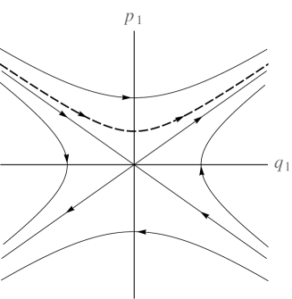
(a) (b)

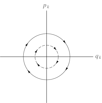
Figure 1: Phase portrait of the phase space. Projections of a reactive trajectory (dashed curves) into (a) the saddle plane, (b) the center planes.

3.2 The general (nonlinear) case

Consider a Hamiltonian $H:\mathbb{R}^{2n}\rightarrow\mathbb{R}$ with an equilibrium at the origin $(q,p)=(0,0)$ for some canonical coordinates $(q,p)$. Assume that $H$ has a saddle-center-…-center stability type equilibrium, that is, the matrix associated with the linearization at $(0,0)$ of the Hamiltonian vector field has eigenvalues $\mp\lambda$, $\lambda>0$, and $\mp\mathrm{i}\,\omega_{k}$, $\omega_{k}>0$, $k=1,\dots,n-1$. Further assume that the submatrix corresponding to the imaginary eigenvalues is semisimple. In the neighborhood of the saddle the dynamics is thus similar to that of the linear vector field described in Sec. 3.1. In fact if follows from general principles that all the phase structures discussed in Sec. 3.1 persist in the neighborhood of the saddle (which in particular implies that one has to restrict to energies close to the energy of the saddle). Moreover, these phase space structures can be constructed in an algorithmic fashion using a Poincaré-Birkhoff normal form [7, 8]. Assuming that the eigenvalues $\omega_{k}$, $k=2,\ldots,n$, are independent over the field of rational numbers (i.e. in the absence of resonances), the Poincaré-Birkhoff normal form yields a symplectic transformation to new (normal form) coordinates such that the transformed Hamiltonian function truncated at order $n_{0}$ of its Taylor expansion assumes the form

$$H_{\text{NF}}({\cal I}_{1},\mathcal{I}_{2},\ldots,\mathcal{I}_{n})\,,$$ (8)

where ${\cal I}_{1}$ and $I_{k}$, $k=2,\ldots,n$, are constants of motions which (when expressed in terms of the normal form coordinates) have the same form as in (5), and $H_{\text{NF}}$ is a polynomial of order $n_{0}/2$ in ${\cal I}_{1}$ and $I_{k}$, $k=2,\ldots,n$ (note that only even orders $n_{0}$ of a normal form make sense).

In terms of the normal form coordinates the phase space structures can be defined in a manner which is virtually identical to the linear case by replacing $H_{2}(q,p)$ by $H_{\mathrm{NF}}({\cal I}_{1},I_{2},\ldots,\mathcal{I}_{n})$ in the definitions in Sec. 3.1. Using then the inverse of the normal form transformation allows one to construct the phase space structures in the original (‘physical’) coordinates. As it is seen the Poincaré-Birkhoff normal form is the main tool in defining phase space structures, but we only review the first order linearization in the next section, as it serves enough for our purpose of stabilization.

4 Stabilization of saddle-type equilibria

In this section we consider a nonlinear Hamiltonian system of reaction-type, and we give a result which gives an algorithmic way of making the system asymptotically stable around the given equilibrium. This is done as follows.

Let $P$ be a Poisson manifold, $(z_{1},\dots,z_{2n})=(x_{1},\dots,x_{n},P_{1},\dots,P_{n})$ be a canonical coordinate system around $z_{0}\in P$ which is set to be the origin $(0,\dots,0)$, and $H:P\rightarrow\mathbb{R}$ be an analytic Hamiltonian function with the corresponding Hamiltonian vector field $X_{H}$ having $z_{0}$ as an equilibrium point of type saddle-center-…-center. So we assume that the linearization matrix of $X_{H}$, or in other words the matrix $J\,D^{2}H$ evaluated at $z_{0}$, has eigenvalues $\mp\lambda,\,\mp\mathrm{i}\,\omega_{k}$, for reals $\lambda,\omega_{k}>0$, $k=2,\dots,n$.

One can put the quadratic part of $H$ into the form (4) by a symplectic change of coordinates [8]. To do this label the eigenvalues by

$$e_{1}=\lambda=-e_{n+1},\quad e_{k}=\mathrm{i}\,\omega_{k}=-e_{k+n},\quad k=2,\dots,n,$$ (9)

and corresponding eigenvalues by $v_{1},\dots,v_{2n}$. Consider the following symplectic matrix

$$M=(c_{1}\,v_{1},c_{2}\,\mbox{Re}v_{2},\dots,c_{n}\,\mbox{Re}v_{n},c_{1}\,v_{1+n},c_{2}\,\mbox{Im}v_{2},\dots,c_{n}\,\mbox{Im}v_{n})$$ (10)

where

$$c_{1}=\langle v_{1},J\,v_{1+n}\rangle^{-1/2},\quad c_{k}=\langle\mbox{Re}v_{k},J\,\mbox{Im}v_{k}\rangle^{-1/2},\quad k=2,\dots,n.$$ (11)

Then the coordinate transformation

$$M\cdot\left[\begin{array}[]{c}x\\ P\end{array}\right]=\left[\begin{array}[]{c}\bar{q}\\ \bar{p}\end{array}\right]$$ (12)

gives a new canonical coordinate system $(\bar{q}_{1},\dots,\bar{q}_{n},\bar{p}_{1},\dots\,\bar{p}_{n})$, and in these coordinates the quadratic part of the Hamiltonian takes the form

$$H_{2}(\bar{q},\bar{p})=\lambda\,\bar{q}_{1}\,\bar{p}_{1}+\sum_{k=2}^{n}\frac{\omega_{k}}{2}(\bar{p}_{k}^{2}+\bar{q}_{k}^{2})\,.$$ (13)

Let a rotation $N$ be given by

$$\begin{split}q_{1}&=\frac{1}{\sqrt{2}}\,\bar{q}_{1}-\frac{1}{\sqrt{2}}\,\bar{p}_{1},\quad p_{1}=\frac{1}{\sqrt{2}}\,\bar{q}_{1}+\frac{1}{\sqrt{2}}\,\bar{p}_{1},\\ q_{k}&=\bar{q}_{k},\quad p_{k}=\bar{p}_{k},\quad k=2,\dots n,\end{split}$$ (14)

then if we introduce

$$S=N\cdot M^{-1}$$ (15)

the coordinate transformation

$$S\cdot\left[\begin{array}[]{c}x\\ P\end{array}\right]=\left[\begin{array}[]{c}q\\ p\end{array}\right]$$ (16)

gives also a set of canonical coordinates $(q_{1}\dots,q_{n},p_{1}\dots,p_{n})$. Then in $(q,p)$ coordinates $H_{2}$ assumes the form (4).

Consider the controls

$$u_{i}=-c\,F_{1}-d_{i}\,\dot{F}_{i},\quad i=1,\dots,n,$$ (17)

with any constants such that $c>\lambda$ and $d_{i}>0,\,i=1,\dots,n$, where the functions $F_{i}:P\rightarrow\mathbb{R}$ are given by

$$F_{i}=\sum_{j=1}^{n}S_{ij}\,z_{j}$$ (18)

for the matrix $S$ introduced in Eq. 15. Then we prove

Theorem 2.

With the notion above, the system

$$\dot{z}=X_{H}(z)-X_{F_{1}}(z)\,u_{1}-\dots-X_{F_{n}}(z)\,u_{n}$$ (19)

is asymptotically stable around $z_{0}$.

Proof.

We want to show that the conditions of Theorem 1 are satisfied. First, it is easily seen that $F_{i}(z_{0})=\sum_{j=1}^{n}S_{ij}\,z_{j}(z_{0})=0$ for $i=1,\dots,n$. Then we add the control $v=-c\,F_{1}$ and consider the new system

$$\dot{z}=X_{H}-X_{F_{1}}(z)\,v.$$ (20)

One can check that the system (20) is also Hamiltonian with the modified Hamiltonian $H_{\mbox{mod}}=H+\frac{1}{2}\,c\,F_{1}^{2}$ and the Hessian matrix $D^{2}H(z_{0})$ is positive definite. In fact,

$$\dot{z}=X_{H}-X_{F_{1}}(z)\,v=X_{H}+c\,X_{F_{1}}(z)\,F_{1}=X_{H}+c\,X_{\frac{1}{2}\,F_{1}^{2}}(z)=X_{H+\frac{1}{2}\,c\,F_{1}^{2}}(z),$$ (21)

and in normal form coordinates $F_{i}=q_{i}$, $i=1,\dots,n$, so in these coordinates

$$D^{2}H_{\mbox{mod}}(q,p)=D^{2}H(q,p)+c\,E_{11},$$ (22)

where $E_{11}$ is the matrix with zero entries except the first entry equal to $1$. This shows that

$$D^{2}H_{\mbox{mod}}(z_{0})=\mbox{diag}(-\lambda+c,\lambda,\omega_{1},\omega_{1},\dots,\omega_{n},\omega_{n}).$$ (23)

which is, clearly, positive definite since $c>\lambda$.

So far, we have ensured the positive definiteness condition in Theorem 1. Next we add the controls $v_{i}=-d_{i}\,\dot{F}_{i}$, $i=1,\dots,n$, and it remains to show that the functions $F_{i}$, $i=1,\dots,n$ satisfy the dimensionality assumption $\mbox{dim}(d\mathcal{C})=2n$ for

$$d\mathcal{C}(z)=\mbox{span}\{dg(z)|g\in\mathcal{C}\},$$ (24)

where

$$\mathcal{C}=\mbox{span}\{F_{i},\{H_{\mbox{mod}},F_{i}\},\{H,\{F_{i}\}\},\dots\},\quad i=1,\dots n,$$ (25)

and $F_{i}$ are in involution. To see this it is observed that

$$\mathcal{C}=\mbox{span}\{q_{i},\{H_{\mbox{mod}}\circ S^{-1},q_{i}\},\{H,\{q_{i}\}\},\dots\},\quad i=1,\dots n.$$ (26)

In fact, by $F_{i}=q_{i}\circ S$ we have

$$\{H_{\mbox{mod}},F_{i}\}=\{H_{\mbox{mod}},q_{i}\circ S\}=\{H_{\mbox{mod}}\circ S^{-1},q_{i}\}$$ (27)

since $S$ is a Poisson map. But $H_{\mbox{mod}}\circ S^{-1}$ is real analytic so we can write it as a Taylor series around $z_{0}$ where the quadratic part is given by (4). Then it can be seen that $f_{i}=\{H_{\mbox{mod}}\circ S^{-1},q_{i}\},\,i=1,\dots,n$, are independent, because one has

$$\begin{split}f_{1}&=\{H_{\mbox{mod}}\circ S^{-1},q_{1}\}=\lambda\,p_{1}+\mbox{h.o.t.},\\ f_{k}&=\{H_{\mbox{mod}}\circ S^{-1},q_{k}\}=\omega_{k}\,p_{k}+\mbox{h.o.t.},\quad k=1,\dots,n.\end{split}$$ (28)

Furthermore, $\{q_{1},\dots,q_{n},f_{1},\dots,f_{n}\}$ forms a set of $2n$ independent functions. So, $d\mathcal{C}(z)$ is $2n$-dimensional, in particular

$$d\mathcal{C}(z_{0})=\mbox{span}\{dq_{1}(z_{0}),\dots,dq_{n}(z_{0}),dp_{1}(z_{0}),\dots,dp_{n}(z_{0})\}.$$ (29)

As the final step we need to show that $F_{i}$ are in involution. This can also be seen easily by

$$\{F_{i},F_{j}\}=\{q_{i}\circ S,q_{j}\circ S\}=\{q_{i},q_{j}\}=0.$$ (30)

∎

The feedback added system is no more conservative because of the dissipative inputs $v_{i}$. As the system is asymptotically stable, trajectories projected into the phase planes look like the ones in Fig. 2.

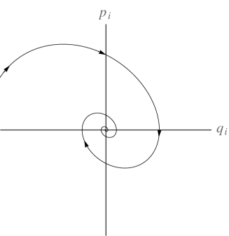
Figure 2: Projetion of trajectories near the equilibrium into the phase planes.

5 Destabilization of a stable system to make a reacting one

A similar procedure as in Sec. 4 can also be applied to a stable system with purely complex eigenvalues in order to obtain an unstable system with a saddle.

We cansider again a Poisson manifold $P$, a canonical coordinate system denoted by $(z_{1},\dots,z_{2n})=(x_{1},\dots,x_{n},P_{1},\dots,P_{n})$ around $z_{0}\in P$ which is set to be the origin $(0,\dots,0)$, and be an analytic Hamiltonian $H:P\rightarrow\mathbb{R}$ with the corresponding Hamiltonian vector field $X_{H}$ having $z_{0}$ as an equilibrium point of type center-…-center. So we assume that the linearization matrix of $X_{H}$, or in other words the matrix $J\,D^{2}H$ evaluated at $z_{0}$, has eigenvalues $\mp\mathrm{i}\,\omega_{i}$, for reals $\omega_{i}>0$, $i=1,\dots,n$.

The quadratic part of the Hamiltonian can be put in the form $H$ into the form

$$H_{2}(q,p)=\sum_{i=1}^{n}\frac{\omega_{i}}{2}(p_{i}^{2}+q_{i}^{2})\,,$$ (31)

by a symplectic change of coordinates [8] as recalled in the following. Label the eigenvalues by

$$e_{i}=\mathrm{i}\,\omega_{i}=-e_{i+n},\quad i=1,\dots,n,$$ (32)

and corresponding eigenvalues by $v_{1},\dots,v_{2n}$. Consider the following symplectic matrix

$$M=(c_{1}\,\mbox{Re}v_{1},\dots,c_{n}\,\mbox{Re}v_{n},c_{1}\,\mbox{Im}v_{1},\dots,c_{n}\,\mbox{Im}v_{n})$$ (33)

where

$$c_{i}=\langle\mbox{Re}v_{i},J\,\mbox{Im}v_{i}\rangle^{-1/2},\quad i=1,\dots,n.$$ (34)

Then the coordinate transformation

$$M\cdot\left[\begin{array}[]{c}x\\ P\end{array}\right]=\left[\begin{array}[]{c}q\\ p\end{array}\right]$$ (35)

gives a new canonical coordinate system $(q_{1},\dots,q_{n},p_{1},\dots\,p_{n})$, and in these coordinates the quadratic part of the Hamiltonian takes the form (31).

Consider the control

$$u=-\,c\,F_{1}$$ (36)

with any constants such that $c>\omega_{1}$ the function $F_{1}:P\rightarrow\mathbb{R}$ is given by

$$F_{1}=\sum_{j=1}^{n}M_{1j}\,z_{j}$$ (37)

for the matrix $M$ introduced in Eq. 35. Then we prove

Theorem 3.

With the notion above, the system

$$\dot{z}=X_{H}(z)-X_{F_{1}}(z)\,u_{1}$$ (38)

is of type $saddle-center-\dots-center$.

Proof.

Similar to the proof of Theorem 2. ∎

6 Examples

We illustrate the procedure of making a saddle-type equilibrium asymptotically stable with two examples.

6.1 A model example

The following system represents a typical pattern of isomerization reactions [12].

Consider a system with potential function

$$V(x_{1},x_{2})=\frac{1}{a^{2}}\,x_{1}^{2}\,(x_{1}-1)^{2}+\frac{1}{b^{2}}\,x_{2}^{2},\quad a>b,$$ (39)

and Hamiltonian

$$H(x_{1},x_{2},P_{1},P_{2})=\frac{1}{2}\,P_{1}^{2}+\frac{1}{2}\,P_{2}^{2}+V(x_{1},x_{2}).$$ (40)

Clearly, $H$ has three equilibria which are critical points of $V$. These are two centers; $(x_{1},x_{2})=(0,0)$ and $(x_{1},x_{2})=(1,0)$, and one saddle; $(x_{1},x_{2})=(1/2,0)$. As we are interested in the saddle, we translate the coordinates by $(x_{1},x_{2})\mapsto(x_{1}+1/2,x_{2})$ to move the saddle to the origin. We use the same notation for the translated coordinates and the potential, then we have

$$V(x_{1},x_{2})=\frac{1}{a^{2}}\,x_{1}^{2}\,(x_{1}-1)^{2}+\frac{1}{b^{2}}\,x_{2}^{2},\quad a>b$$ (41)

which will be used henceforth. The contours of the potential surface are depicted in Fig. 3.

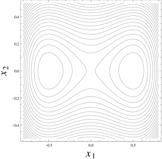
(a) (b)

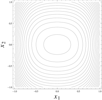
Figure 3: Contours of potential functions; (a) the original model potential (41), (b) the modified potential (46).

The Hessian matrix $J\,D^{2}H$ at point $z_{0}=(0,0,0,0)$ is computed to be

$$J\,D^{2}H(z_{0})=\left[\begin{array}[]{cccccc}0&0&1&0\\ 0&0&0&1\\ \frac{1}{a^{2}}&0&0&0\\ 0&-\frac{2}{b^{2}}&0&0\\ \end{array}\right]$$ (42)

which has eigenvalues $e_{1}=\frac{1}{a}=-e_{3},\quad e_{2}=\frac{\sqrt{2}}{b}\,\mathrm{i}=-e_{4}$ with corresponding eigenvectors $v_{1}=\{a,0,1,0\},\,v_{3}=\{-a,0,1,0\},\,v_{2}=\{0,-\frac{b}{\sqrt{2}}\,\mathrm{i},0,1\},\,v_{4}=\{0,-\frac{b}{\sqrt{2}}\,\mathrm{i},0,1\}$. So, we have $c_{1}=(v_{1}\cdot J\,v_{3})^{-1/2}=(2\,a)^{-1/2},\,c_{2}=(\mbox{Re}(v_{2})\cdot J\,\mbox{Im}(v_{2}))^{-1/2}=2^{1/4}\,b^{-1/2}.$ Then the matrix $M$ reads

$$M=\left[\begin{array}[]{cccccc}\frac{\sqrt{a}}{\sqrt{2}}&0&-\frac{\sqrt{a}}{\sqrt{2}}&0\\ 0&0&0&-\frac{\sqrt{b}}{2^{1/4}}\\ \frac{1}{\sqrt{2\,a}}&0&\frac{1}{\sqrt{2\,a}}&0\\ 0&\frac{2^{1/4}}{\sqrt{b}}&0&0\\ \end{array}\right].$$ (43)

Finally, the matrix $S$ which is the multiplication of the rotation matrix

$$R=\left[\begin{array}[]{cccccc}\frac{1}{\sqrt{2}}&0&-\frac{1}{\sqrt{2}}&0\\ 0&0&0&0\\ \frac{1}{\sqrt{2}}&0&\frac{1}{\sqrt{2}}&0\\ 0&0&0&0\\ \end{array}\right]$$ (44)

and the matrix $M$ becomes

$$S=\left[\begin{array}[]{cccccc}\frac{1}{\sqrt{a}}&0&0&0\\ 0&0&0&\frac{\sqrt{b}}{2^{1/4}}\\ 0&0&\sqrt{a}&0\\ 0&-\frac{2^{1/4}}{\sqrt{b}}&0&0\\ \end{array}\right].$$ (45)

Hence the functions $F_{1},F_{2}$ are obtained to be $F_{1}=\frac{x_{1}}{\sqrt{a}},\,F_{2}=\frac{\sqrt{b}}{2^{1/4}}\,P_{2}$. Observe that, the modified Hamiltonian $H_{\mbox{mod}}$ has the form $H_{\mbox{mod}}=H+\frac{1}{2\,a^{2}}\,x_{1}^{2}$, and the modified potential is

$$V_{\mbox{mod}}=V+\frac{1}{2\,a^{2}}\,x_{1}^{2}$$ (46)

of which contours are depicted in Fig. 3 (b). After the addition of associated controls, we have the system with equations of motion

$$\begin{split}\dot{x}_{1}&=P_{1},\\ \dot{x}_{2}&=P_{2}+\frac{\sqrt{2}\,x_{2}}{b},\\ \dot{P}_{1}&=-\frac{4\,x_{1}^{3}}{a^{2}}+\frac{P_{1}}{a},\\ \dot{P}_{2}&=-\frac{2\,x_{2}}{b^{2}},\end{split}$$ (47)

where we choose $d_{1}=d_{2}=1$.

6.2 Hydrogen atom in crossed and magnetic fields

The following example is a Hamiltonian system which is not of the form kinetic plus potential. We do not give the original form but a form obtained after some manipulations [7].

The Hamiltonian can be put in the form

$$H=\frac{1}{2}\,(P_{1}^{2}+P_{2}^{2}+P_{3}^{2})-\frac{1}{R}+\frac{1}{2}\,(x_{1}\,P_{2}-x_{2}\,P_{1})+\frac{1}{8}\,(x_{1}^{2}+x_{2}^{2})-\epsilon\,x_{1},$$ (48)

where $R=(x1^{2}+x_{2}^{2}+x_{3}^{2})^{1/2}$. We will consider the experimentally interesting value $\epsilon=0.58$ henceforth. The Stark saddle point in atomic physics corresponds to the point $(x_{1},x_{2},x_{3},P_{1},P_{2},P_{3})=(\epsilon^{1/2},0,0,0,-\frac{1}{2}\,\epsilon^{-1/2})$. So after a coordinate shift $(x_{1},x_{2},x_{3},P_{1},P_{2},P_{3})\mapsto(x_{1}-\epsilon^{1/2},x_{2},x_{3},P_{1},P_{2},P_{3}+\frac{1}{2}\,\epsilon^{-1/2}),$ by retaining the same notation for the translated coordinates and the new Hamiltonian we have

$$H=\frac{1}{2}\,(P_{1}^{2}+P_{2}^{2}+P_{3}^{2})-\frac{1}{R}+\frac{1}{2}\,(x_{1}\,P_{2}-x_{2}\,P_{1})+\frac{1}{8}\,(x_{1}^{2}+x_{2}^{2})-\epsilon\,x_{1}-\epsilon^{1/2},$$ (49)

where $R=\left[(x_{1}+\epsilon^{1/2})^{2}+x_{2}^{2}+x_{3}^{2}\right]^{1/2}$. Then the matrix $J\,D^{2}H(0)$ is obtained to be

$$J\,D^{2}H(0)=\left[\begin{array}[]{cccccc}0&-0.5&0&1&0&0\\ 0.5&0&0&0&1&0\\ 0&0&0&0&0&1\\ 0.63343&0&0&0&-0.5&0\\ 0&-0.691715&0&0.5&0&0\\ 0&0&-0.441715&0&0&0\end{array}\right]$$ (50)

which has eigenvalues

$$e_{1}=0.63645=-e_{4},\quad e_{2}=0.981506\,\mathrm{i}=-e_{5},\quad e_{3}=0.664616\,\mathrm{i}=-e_{6}$$ (51)

with corresponding eigenvectors

$$\begin{split}v_{1,4}&=\{\pm 0.63645,0.478361,0,0.644249,\mp 0.0137719,0\},\\ v_{2,5}&=\{\pm 0.981506\,\mathrm{i},1.84678,0,-0.0399619,\pm 1.32188\,\mathrm{i},0\},\\ v_{3,6}&=\{0,0,\mp 1.50463\,\mathrm{i},0,0,1\}.\end{split}$$ (52)

So, we have

$$\begin{split}c_{1}&=(v_{1}\cdot J\,v_{4})^{-1/2}=1.09551,\\ c_{2}&=(\mbox{Re}(v_{2})\cdot J\,\mbox{Im}(v_{2}))^{-1/2}=0.634944\\ c_{3}&=(\mbox{Re}(v_{3})\cdot J\,\mbox{Im}(v_{3}))^{-1/2}=0.81524.\end{split}$$ (53)

Then the matrix $M$ reads

$$M=\left[\begin{array}[]{cccccc}0.697235&0&0&-0.697235&0.623201&0\\ 0.524048&1.1726&0&0.524048&0&0\\ 0&0&0&0&0&-1.22663\\ 0.705779&-0.0253736&0&0.705779&0&0\\ -0.0150872&0&0&0.0150872&0.839317&0\\ 0&0&0.81524&0&0&0\\ \end{array}\right].$$ (54)

Finally, the matrix $S$ which is the multiplication of the rotation matrix $R$ and the matrix $M$ becomes

$$S=\left[\begin{array}[]{cccccc}0.998122&0&0&0&-0.741116&0\\ 0&0.839317&0&-0.623201&0&0\\ 0&0&0&0&0&1.22663\\ 0&0.0213366&0&0.986039&0&0\\ 0.0253736&0&0&0&1.1726&0\\ 0&0&-0.81524&0&0&0\\ \end{array}\right].$$ (55)

Hence the functions $F_{1},F_{2},F_{3}$ are derived as

$$\begin{split}F_{1}&=-0.741116\,P_{2}+0.998122\,x_{1},\\ F_{2}&=-0.623201\,P1+0.839317\,x_{2},\\ F_{3}&=1.22663\,P_{3}.\end{split}$$ (56)

This way, the new system is made asymptotically stable around the origin.

7 Conclusions and future work

An algorithmic stabilization of reacting systems is outlined. It relays on the linearization of the Hamiltonian vector field around the equilibrium. The examples reflect the novelty of the technique given in the paper. Next step is to do a study for Hamiltonian systems with symmetry where the equilibria are replaced by relative equilibria. This can be done by using canonical coordinates on the reduced space instead of the reduced energy momentum method as in [3]. A derivation method of canonical coordinates on a reduced space for $N$-body reduction is outlined in [10] and for cotangent bundle reduction is given in [13].

References

- [1] E. D. Sontag. Feedback stabilization of nonlinear systems. In Mathematical Theory of Networks and Systems. Birkhauser, pages 61–81. Birkhauser, 1989.
- [2] H. Nijmeijer and A. van der Schaft. Nonlinear dynamical control systems. Springer-Verlag, New York, 1990.
- [3] S. M. Jalnapurkar and J. E. Marsden. Stabilization of relative equilibria. IEEE Trans. Automat. Control, 45(8):1483–1491, 2000.
- [4] A. M. Bloch, N. E. L.eonard, and J. E. Marsden. Controlled Lagrangians and the stabilization of mechanical systems. I. The first matching theorem. IEEE Trans. Automat. Control, 45(12):2253–2270, 2000.
- [5] A. M. Bloch, D. E. Chang, N. E. Leonard, and J. E. Marsden. Controlled Lagrangians and the stabilization of mechanical systems. II. Potential shaping. IEEE Trans. Automat. Control, 46(10):1556–1571, 2001.
- [6] R. Krechetnikov and J. E. Marsden. Dissipation-induced instabilities in finite dimensions. Rev. Mod. Phys., 79:519–553, Apr 2007.
- [7] T. Uzer, C. Jaffé, J. Palacián, P. Yanguas, and S. Wiggins. The geometry of reaction dynamics. Nonlinearity, 15:957–992, 2002.
- [8] H. Waalkens, R. Schubert, and S. Wiggins. Wigner’s dynamical transition state theory in phase space: classical and quantum. Nonlinearity, 21(1):R1–R118, 2008.
- [9] S. M. Jalnapurkar. Modeling and stabilization for mechanical systems. ProQuest LLC, Ann Arbor, MI, 1999. Thesis (Ph.D.)–University of California, Berkeley.
- [10] Ü. Çiftçi and H. Waalkens. Phase space structures governing reaction dynamics in rotating molecules. Nonlinearity, 25:791–892, 2012.
- [11] S. Wiggins. Normally Hyperbolic Invariant Manifolds in Dynamical Systems. Springer, Berlin, 1994.
- [12] A. Tachibana and K. Fukui. Differential geometry of chemically reacting systems. Theoretica chimica acta, 49:321–347, 1978.
- [13] Ü. Çiftçi, H. Waalkens, and H. Broer. Cotangent bundle reduction and Poincaré-Birkhoff normal forms. Preprint.