Information sharing in Quantum Complex Networks

Abstract

We introduce the use of entanglement entropy as a tool for studying the amount of information shared between the nodes of quantum complex networks. By considering the ground state of a network of coupled quantum harmonic oscillators, we compute the information that each node has on the rest of the system. We show that the nodes storing the largest amount of information are not the ones with the highest connectivity, but those with intermediate connectivity thus breaking down the usual hierarchical picture of classical networks. We show both numerically and analytically that the mutual information characterizes the network topology. As a byproduct, our results point out that the amount of information available for an external node connecting to a quantum network allows to determine the network topology.

I Introduction

The advent of network science has influenced the research in many fields of science in general, and physics in particular, in a pervasive way barabasi . Since the discovery of the structural features of real social, biological and technological networks rev:albert ; rev:newman , the development of the theoretical machinery of network science has blossomed as an efficient framework to interpret the many interaction patterns encoded in real-scale complex systems of diverse nature newman_book and to model correctly the dynamical processes taking place on top of them rev:bocc ; vespignani .

One of the most important avenues of research in network science is its connection with information theory. In this way, different information-theoretical tools have been proposed to characterize the complexity of networks beyond the typical statistical indicators such as their degree distribution, clustering coefficient, degree correlations, etc newman_book . For instance, Shannon entropy, as shown in GB1 ; GB2 ; GB3 ; Marro ; Braunstein ; GB0 , has been successfully applied to characterize the complexity of ensembles of networks sharing some structural features while information-theoretical tools have been also applied to the study of diffusion processes on top of networks, such as random walks ER1 ; ER2 ; ER3 ; GB ; rosvall1 ; rosvall2 .

The synergy between the field of complex networks and that of information theory has recently appealed to the quantum information community Ferraro ; Garnerone2012b . As a product, classical results on percolation theory QPercAcin ; QPercCuquet1 ; QPercCuquet2 ; QPercWu and network science, such as the small-world effect QSW , have been revisited in networked structures of coupled quantum systems as a first step for designing quantum communication networks. Conversely, the use of quantum dynamical processes, such as quantum random walks muelken ; Almeida2012 and their application to rank the importance of network elements QRsilvano ; QRpaparo ; QRburillo ; Garnerone2012 , has given new quantum information perspectives to classical problems of the network realm.

The most fundamental characterization of a network is its connectivity distribution $P(k)$, i.e., the probability of finding a node connected to $k$ other nodes of the network. In addition to $P(k)$, many other statistical quantities in network scienceare used to characterize the topology relying on the sampling of the local measures (such as the degree $k$) of nodes newman_book . On the other hand, quantum mechanical states built as ground states of many body Hamiltonians rely on both local and global lattice properties. As a consequence, the characterization of nodes’ states in quantum complex network offers the possibility of extracting a novel characterization of nodes attributes, beyond those present in their local neighborhood.

In this work we quantify the amount of mutual information that a single node shares with the rest of the network. To this aim, we compute the vacuum state of bosonic modes harmonically coupled through the specific adjacency matrix of a given complex network. We first show that the information contained in each node or lattice point is particularly characteristic (the precise meaning of which to be specified later) of the whole topology and, second , that hubs (nodes with the largest connectivity) become isolated in terms of the mutual information shared with the rest of the network. Both features are equally surprising from the point of view of the classical network paradigm but, as we will discuss here, natural when quantum effects are incorporated. It is important to stress that both the models and the topologies studied here are far from solely being a fundamental curiosity. In fact, non regular topologies in quantum models, as those described here, are currently investigated in different contexts such as quantum emergent gravity models Caravelli2012 , Anderson localization Sade2005 ; Jahnke2008 , quantum phase transitions Halu2013 or optical communications Shapiro1982 .

II Theory and Model

As usual, we define a network as a set of $N$ nodes and $E$ edges (or links) accounting for their pairwise interactions. The network ‘backbone’ is usually encoded in the Adjacency matrix, $A$, such that $A_{ij}=1$ if an edge connects nodes $i$ and $j$ while $A_{ij}=0$ otherwise. In this work we restrict to undirected networks so that $A_{ij}=A_{ji}$. Although matrix $A$ stores all the structural meaning of a network it is more convenient to rely on the so-called network Laplacian, $L$, to analyze its structural and dynamical properties spectra . The Laplacian of a network is defined from the Adjacency matrix as $L_{ij}=k_{i}\delta_{ij}-A_{ij}$, where $k_{i}=\sum_{j}A_{ij}$ is the connectivity of node $i$, i.e., the number of nodes connected to $i$.

A quite minimalistic manner to translate the features of a given Laplacian into a quantum system is to consider identical, unit mass, quantum harmonic oscillators with equal on-site frequency (normalized to $1$), and interacting via springs as dictated by the adjacency matrix, the potential being $V=\sum_{i,j}cA_{i,j}(x_{i}-x_{j})^{2}/2$. The resulting Hamiltonian of the quantum network can be written then:

$$H_{\rm network}=\frac{1}{2}\Big{(}{\bf p}^{\rm T}{\bf p}+{\bf x}^{\rm T}(\mathbb{I}+2cL){\bf x}\Big{)}\,,$$ (1)

where $x_{j}=\frac{1}{\sqrt{2}}(a_{j}+a_{j}^{\dagger})$ and $p_{j}=\frac{i}{\sqrt{2}}(a_{j}-a_{j}^{\dagger})$ with the bosonic anhilitation/creation operators satisfying the usual commutation relations $[a_{i},a_{j}^{\dagger}]=\delta_{ij}$ (we set $\hbar=1$). As for a spring coupling matrix, the Laplacian guarantees $H_{\rm network}\geq 0$ and therefore the existence of a ground state. Finally, we have included in the model a global coupling strength, $c$, which is somehow arbitrary. Our conclusions are independent of $c$ and it can be seen as a regularization term fn1 . The problem, despite quantum, is harmonic and therefore it is simple enough to attack a complex topology and compute its ground state. Almost any other Hamiltonian would make it impossible to perform the exact calculation of its ground state in a complex topology. Therefore Eq. (1) is a minimal numerically solvable model. In particular its ground state, the vacuum, relies on the eigenvectors of the Laplacian matrix and their corresponding eigenvalues shifted by $1$. As a final note, let us comment that the classical limit of (1) has a trivial ground state: all the nodes having $x_{i}=p_{i}=0$ independent on the topology. Therefore the quantum model, in this sense, is not trivial. Then all the ground state mutual information, if any, shared by a node with the rest of the network is then due to quantumness.

Figure 1: (color online) Connectivity distribution $P(k)$ for scale free networks: Configurational (SF-CONF) (a) and Barabási-Albert Scale-Free (SF-BA) (b). Figures (c) and (d) stand for Erdős-Rényi (ER) and Random Regular Graphs (RRG).

We now quantify the amount of information each of the elements of a network shares with the rest of the system. To this aim, we consider the partition of the network into a node, say $i$, and its complement $i^{\rm c}$, i.e. the rest of the network. Then, we compute the mutual information shared by the two parties as:

$${\mathcal{I}}(i|i^{\rm c})=S_{i}+S_{i^{\rm c}}-S_{\rm tot}\;.$$ (2)

Here $S_{i}$ and $S_{i^{\rm c}}$ are marginal (von Neumann) entropies and $S_{\rm tot}$ is the total entropy of the network.

Since the total network is in its ground (hence pure) state we have $S_{\rm tot}=0$ and $S_{i}=S_{i^{\rm c}}=\mathcal{I}(i|i^{\rm c})/2$. Therefore, the information that a node shares with the network is intrinsically due to quantum correlations. Equivalently, the mutual information is itself a measure of the entanglement (twice the entropy of entanglement, quantified by $S_{i}$) between a single node and the rest of the system. The marginal entropies for $i$ and $i^{c}$ read Agarwal1971 :

$$\!\!\!\!S_{i}=S_{i^{\rm c}}=\Bigl{(}\!\mu_{i}+\frac{1}{2}\Bigr{)}\log\Bigl{(}\!\mu_{i}+\frac{1}{2}\Bigr{)}-\Bigl{(}\!\mu_{i}-\frac{1}{2}\Bigr{)}\log\Bigl{(}\!\mu_{i}-\frac{1}{2}\Bigr{)}\,,$$ (3)

which is a monotonically increasing function of $\mu_{i}$ that is characterized by the second moments of the positions and momenta of nodes, $\mu_{i}=\sqrt{\langle x_{i}^{2}\rangle\langle p_{i}^{2}\rangle}$. After some algebra (see Appendix A) we are able to quantify the value of $\mu_{i}$ as:

$$\mu_{i}^{2}=\frac{1}{4}\sum_{j,j^{\prime}}S_{ij}^{2}S_{ij^{\prime}}^{2}\sqrt{\frac{1+2c\lambda_{j}}{1+2c\lambda_{j^{\prime}}}}\;,$$ (4)

where $\{\lambda_{j}\}$ are the eigenvalues of the network Laplacian $L$ and matrix $S$ accounts for the normal mode transformation that diagonalizes the network Laplacian: $L_{d}=S^{T}LS$ with $S^{T}S={\mathbb{I}}$.

From Eq.(3) it is clear that each node has some mutual information with the rest of the system provided $\mu_{i}>1/2$ whereas from Eq.(4) we conclude that the amount of information depends on its contribution to each of the Laplacian eigenvectors.

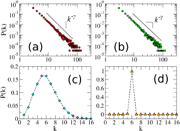
In the following we quantify the entanglement entropies of nodes embedded in different network topologies. First, we explore two homogeneous network substrates: (i) Random Regular Graphs (RRG), in which all the nodes have the same number of contacts ($k_{i}=\langle k\rangle,\forall i$), and (ii) Erdős-Rényi (ER) networks er , for which the probability of finding a node with $k$ neighbors, $P(k)$, follows a Poisson distribution so that most of the nodes have a degree $k$ close to the average $\langle k\rangle$. Besides, we have analyzed networks having a scale-free (SF) pattern for the probability distribution, $P(k)\sim k^{-3}$, constructed by means of a configurational random model (SF-CONF) conf and the Barabási-Albert model (SF-BA) ba (see Figure 1).

III Mutual information

We move to the numerical study and discussion of our results in all those different complex network topologies. To this aim, we collect the entanglement entropies of the $N_{k}$ nodes having connectivity $k$ and define the average entanglement of the degree class $k$ as: $\langle S_{k}\rangle=\sum_{i|k_{i}=k}S_{i}/N_{k}$. One would expect that the larger the connectivity $k$ of a node the more correlated it is with the rest of the network, and thus the larger the value of $\langle S_{k}\rangle$.

Figure 2: (color online) In (a) we show the microscopic picture: a particular node and its boundary (first neighbors) with the rest of the system (blurred). The rest of the panels show the average entropy of nodes with degree $k$, $\langle S_{k}\rangle$ for the following topologies: (b) ER, (c) SF-CONF and (d) SF-BA networks. Each symbol refers to a value of the coupling strength $c$. In particular, we have that $\bullet$,$\blacksquare$,$\blacklozenge$,$\blacktriangle$ correspond to $c=0.2$, $0.4$, $0.6$ and $0.8$ respectively. All the networks have the same average degree $\langle k\rangle=4$. Solid lines represent the theoretical curves calculated using the mean-field formulation. The fitted values for $\kappa$ are $\kappa=3.8,3.5,4.2$ for the ER, SF-BA and SF-CONF respectively. All the results are averaged over 30 realizations of each kind of network.

Figure 3: (color online) Average entropy of nodes with degree $k$, $\langle S_{k}\rangle$, for all the topologies under study: (a) RRG , (b) ER, (c) SF-CONF and (d) SF-BA networks. All the oscillators are coupled with the same strength $c=0.6$. Each symbol represents a different value of the average degree $\langle k\rangle$ of the system. Solid lines represent the theoretical behavior calculated with the mean-field formulation. The fitted values for$\kappa$ for ER $\kappa=2.6,3.8,5.5$, for SF-BA $\kappa=1.8,3.5,5.2$ and SF-CONF $\kappa=2.5,4.2,5.8$. All the results are averaged over 30 realizations of each kind of network.

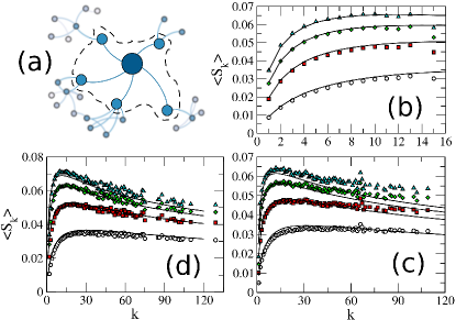
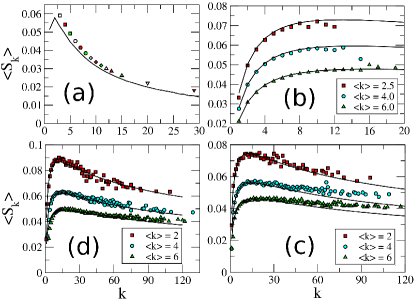
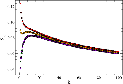
The panels in Figs. 2 and 3 summarize our findings for the behavior of $\langle S_{k}\rangle$. In Fig, 2 we explore ER [panel (b)], SF-CONF [panel (c)] and SF-BA [panel (d)] networks for different values of the coupling $c=0.2,0.4,0.6$ and $0.8$. For ER networks we observe that the value of $\langle S_{k}\rangle$ increases with $k$ although we note that the growing trend seems to saturate for large values of $k$ pointing out that entanglement is bounded. On the other hand for SF networks, displaying a larger heterogeneity for the collection of degrees, the growing trend of $\langle S_{k}\rangle$ only holds for small to moderate connectivities $k$, then $\langle S_{k}\rangle$ reaches a maximum and starts to decrease. Eventually, those nodes with sufficiently large $k$ would drop its entanglement entropy. As a result hubs are not the most entangled nodes, but there is an optimally-correlated class of nodes having moderate connectivity. The plots in Fig. 3 confirm the above results. In these cases, we have fixed $c=0.6$ and changed the mean connectivity of the RRG [panel (a)], ER [panel (b)], SF-CONF [panel (c)] and SF-BA [panel (d)] networks. Notice that in the RRG the mean connectivity and the connectivity are the same (all the nodes have the same connectivity, see Fig. 1). Therefore, considering a net with some $\langle k\rangle$ would provide only one point in the curve $\langle S_{k}\rangle$, so we merge in one plot different networks with different connectivities.

IV Mean-field formulation

In the following we develop a minimal model aimed at capturing the rise-and-fall behavior of $\langle S_{k}\rangle$ in SF networks. The simplest framework to deal with bipartite entanglement is sketched in Fig. 2.(a). Rather than selecting a site $i$ and replacing the interaction with each of its neighbors by a mean value (standard mean field), we consider both $i$ and its neighbors. The mean field approximation enters when replacing the interaction of the neighbors of $i$ with their corresponding neighbors by its mean value. This mean field assumption is equivalent to a renormalization of the frequency of the $k$ neighbors of $i$. In this way, the mean field Hamiltonian for a node $i$ with $k$ neighbors yields:

$$H_{\rm MF}^{k}=\frac{1}{2}(p_{i}^{2}+x_{i}^{2})+\frac{1}{2}\sum_{j=1}^{k}p_{j}^{2}+\nu^{2}_{\kappa}x_{j}^{2}+c(x_{i}-x_{j})^{2}\,,$$ (5)

where the renormalized frequency of the neighbors reads: $\nu^{2}_{\kappa}=1+2c\kappa$, and $\kappa$ is a fitting parameter (see below).

This model is analytically solvable (see Appendix B). Therefore, we can find the entropy of the central node $\langle S_{k}\rangle^{MF}$ analytically as a function of its connectivity $k$ and $\kappa$. In Figs. 2 and 3 we plot with solid lines the curves $\langle S_{k}\rangle^{MF}$ obtained after tuning the single parameter $\kappa$ for each of the curves. Our mean-field approximation agrees fairly good with the numerics. The values of $\kappa$ for the different topologies under study are shown in Table 1. As observed, in the case of Erdős Rényi (ER) networks with average degree $\langle k\rangle=2$ results are missing. This is due to the fact that for average degrees lesser than 2.5 the resulting ER networks are not made by a unique connected component. Importantly, we observe that $\kappa$ only depends on the average degree and on the considered underlying topology as it is independent of the coupling parameter $c$ (see Figs. 2 and 3).

In addition to the quantitative agreement, the analytical estimation $\langle S_{k}\rangle^{MF}$ allows to explain the rise-and-fall of entropy across degree classes.

$\langle k\rangle$ \$c$	RRG	ER	SF-BA	SF-CONF
2 \0.2	–	2.6	1.8	2.5
2 \0.4	–	2.6	1.8	2.5
2 \0.6	–	2.6	1.8	2.5
2 \0.8	–	2.6	1.8	2.5
4 \0.2	3.4	3.8	3.5	4.2
4 \0.4	3.4	3.8	3.5	4.2
4 \0.6	3.4	3.8	3.5	4.2
4 \0.8	3.4	3.8	3.5	4.2
6 \0.2	5.2	5.5	5.2	5.8
6 \0.4	5.2	5.5	5.2	5.8
6 \0.6	5.2	5.5	5.2	5.8
6 \0.8	5.2	5.5	5.2	5.8

Table 1: Fitting parameter $\kappa$ for all the different network topologies with respect to each pair of parameters, namely: average degree $\langle k\rangle$ and coupling $c$.

As shown in the Appendix B, this phenomenon lies in the fact that hubs are almost eigenvectors of the Laplacian and thus normal modes of the Hamiltonian (uncoupled from the rest of the system and therefore not entangled). The progressive localization of the eigenvectors with $k$ balances the growth of the correlations associated to the increase of $k$. It is the competition between these two effects what explains the peak for $\langle S_{k}\rangle$ in SF networks at moderately, rather that maximally, coupled nodes.

Figure 4: (color online) Entropy share by an external (blue) node coupled to an ER graph. In the plot we show (filled dots) the entanglement entropy $\langle S_{k}\rangle$ of the nodes of the ER network as a function of their connectivity. In addition, we show (empty squares) the evolution of the entanglement of the external node as a function of its connectivity, i.e. the number of links launched to the target network.

V Attaching an external node

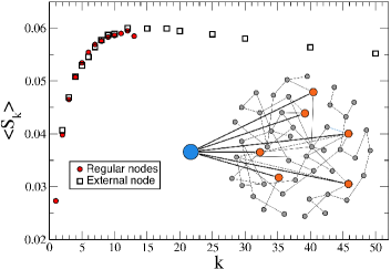
Let us now tackle the problem from a different perspective. Up to this point we have assumed that we have access to any of the nodes and thus computed their corresponding mutual information to characterize the network. Now, we consider the network as an unknown system and aim at recovering the above results by using a single node that can be attached to the network with as many links as desired. If such node/probe could get further information about its own entropy, say by measuring its purity, it could sequentially connect to more and more nodes in a random way so to reproduce a curve $\langle S_{k}\rangle$. We have represented this situation in Fig. 4, for an ER graph, as compared to the situation in which no probe is present. As shown, the external probe realizes, by launching more than $k\simeq 15$ links, that the amount of information it can extract from a the network is bounded and its maximum is reached by means of a moderate number of connections. We note that this individual entropy fairly coincides with the entropy that any internal node of the same connectivity would measure.

Figure 5: (color online) Rise and fall behavior for finite temperature. We plot the expected $S_{k}$ for our mean field description with the values $c=0.6$ and $\kappa=2$, and temperatures $T=0.001$ (green $\blacktriangle$), $0.1$ (purple $\blacksquare$), $0.25$ (orange $\bullet$), $0.3$ (red $\blacklozenge$).

VI Robustness against temperature

We use our mean field approach to explore the effect of temperature on the observed behavior at zero temperature. Instead of assuming the ground state of the network, we take a Gibbs density matrix $\rho=\exp(-H_{\rm net}/T)/Z$ with temperature $T$, $Z={\rm Tr}[\exp(-H_{\rm net}/T)]$ the partition function and we have set $k_{\rm B}=1$. Figure 5 shows the result for $c=0.6$ and fitting parameter $\kappa=2$: the rise and fall behavior survives for $T=0.1$ and starts to disappear only when $T>0.25$. Furthermore, nodes with high connectivity are left almost unaffected by a temperature increase. Indeed, highly connected nodes become almost eigenmodes of the system and their frequency gets renormalized by $k$, meaning that their frequency is very high as compared to temperature. Effectively they do not feel the temperature increase. In contrast, nodes with low connectivity do not feel this renormalization so much, thus leading to the typical increase of entropy due to temperature. In conclusion, the fact that for $T=0.1$ the curve matches the zero temperature one confirm the desired stability for our results and conclusions.

VII Conclusions

The entropy of entanglement of nodes in quantum oscillators networks reveals a novel and non trivial characterization of single node attributes. In particular, the decay of the entanglement for large connectivity nodes is seen as the fingerprint of the localization of some of the Laplacian eigenvectors around hubs which turns them into normal modes of the system. This effect balances the increase of the entanglement with the connectivity, analogously to an area law in regular lattices, thus causing the rise-and-fall of the entanglement entropy across connectivity classes. We further stress that the results presented here survive in presence of a finite, but small temperature.

In addition to their interest for the emerging field of quantum information on networks, our results show an interesting connection with fundamental concepts of quantum gravity in complex spatial connectivities. In fact, the setup used here can be seen as the discretized version of real massive Klein-Gordon fields far from the usual Minkowsky or curved space-time situations, suggested from emergent gravity concepts as intermediate topologies in the transition from a highly connected (high energy) quantum geometric phase of the universe to the low energy, largely homogeneous, actual phase smolin . If the links of the network (related to the quantum gravitational field) are seen as a heat bath for quantum fields ‘living’ on it, the effect of different entropy densities could lead to entropic forces, and therefore to preference of some topological configurations over others. Although the connection between complex space-time topologies and the field of network science has recently attracted attention cosmo , any result coming from this synergy has to be considered preliminary and thought-provoking.

Appendix A Entanglement entropy

Let us start by deriving Eq. (4) in the text. Given $\varrho$, the quantum state of the network, its associated Von Neumann entropy is given by,

$$S=-{\rm Tr}(\varrho\ln\varrho)\;,$$ (6)

where ${\rm Tr}$ accounts for the trace operation. The marginal entropy for the node $i$, $S_{i}$, is obtained by replacing $\varrho$ in (6) by the reduced density matrix,

$$\varrho_{i}={\rm Tr}_{i^{\rm c}}\varrho\;,$$ (7)

where ${\rm Tr}_{i^{\rm c}}$ is the partial trace, i.e., the trace over the complement of $i$ (the rest of the nodes).

In our work, the state of the network considered is the ground state of the Hamiltonian [Eq. (1) in the text]:

$$H_{\rm network}=\frac{1}{2}\Big{(}{\bf p}^{\rm T}{\bf p}+{\bf x}^{\rm T}(\mathbb{I}+2cL){\bf x}\Big{)}\,,$$ (8)

here $\mathbb{I}$ is the $N\times N$ identity matrix, $c$ is the coupling strength between connected oscillators and $L$ the network Laplacian. The operators ${\bf p}^{\rm T}=(p_{1},p_{2},...,p_{N})$ and ${\bf x}^{\rm T}=(x_{1},,x_{2},...,x_{N})$ are the momenta and positions of nodes respectively, satisfying the usual commutation relations: $[{\bf x},{\bf p}^{\rm T}]={\mbox{i}}\hbar\,\mathbb{I}$. We are interested in analyzing the ground state of the system, which is a pure state, thus having $S=0$. On top of that, this state is Gaussian (since the Hamiltonian is quadratic) so that the reduced density matrices $\varrho_{i}$ and $S_{i}$ can be computed by means of the covariance matrix:

$$\sigma=\left(\begin{array}[]{cc}\langle x_{i}^{2}\rangle&\frac{1}{2}\langle x_{i}p_{i}+p_{i}x_{i}\rangle\\ \frac{1}{2}\langle x_{i}p_{i}+p_{i}x_{i}\rangle&\langle p_{i}^{2}\rangle\end{array}\right)\;,$$ (9)

where the averages are calculated via the reduced density matrix, $\varrho_{i}$, as: $\langle x_{i}^{2}\rangle={\rm Tr}(x_{i}^{2}\varrho_{i})$. It was Agarwal Agarwal1971 who derived an explicit formula for the marginal entropies [Eq. (3) in the text]:

$$\!\!\!\!S_{i}=S_{i^{\rm c}}=\Bigl{(}\!\mu_{i}+\frac{1}{2}\Bigr{)}\log\Bigl{(}\!\mu_{i}+\frac{1}{2}\Bigr{)}-\Bigl{(}\!\mu_{i}-\frac{1}{2}\Bigr{)}\log\Bigl{(}\!\mu_{i}-\frac{1}{2}\Bigr{)}\,,$$ (10)

with $\mu_{i}=\sqrt{\langle x_{i}^{2}\rangle\langle p_{i}^{2}\rangle}$.

We are able to find these quadratures by working with normal modes, i.e., those diagonalizing the potential energy matrix $V=\mathbb{I}+2cL$:

$${\bf x}=S\,{\bf Q}\ \textrm{so that}\ S^{\rm T}VS=V_{d},$$ (11)

whose quadratures are those of a set of uncoupled oscillators at their individual ground state:

$$\langle Q_{i}\rangle=\langle P_{i}\rangle = 0$$ (12)

$$\langle Q_{i}Q_{j}\rangle = \delta_{ij}\frac{\hbar}{2\Omega_{j}}$$ (13)

$$\langle P_{i}P_{j}\rangle = \delta_{ij}\frac{\hbar\Omega_{j}}{2}$$ (14)

$$\frac{1}{2}\langle Q_{i}P_{j}+Q_{j}P_{i}\rangle = 0,$$ (15)

with $\Omega_{i}=\sqrt{1+2c\lambda_{i}}$ the eigenfrequencies, and $\lambda_{i}$ the eigenvalues of the Laplacian matrix $L$. The latter relation is obtained from simple inspection of the eigenvalue equation $V{\bf u}=\Omega^{2}{\bf u}=(\mathbb{I}+2cL){\bf u}$, so that $L{\bf u}=\frac{\Omega^{2}-1}{2c}{\bf u}\equiv\lambda{\bf u}$. That is, ${\bf u}$ is an eigenvector of both $V$ and $L$, with $\Omega=\sqrt{1+2c\lambda}$. Then we obtain:

$$\langle x_{i}\rangle =\sum_{j}S_{ij}\langle Q_{j}\rangle=0$$ (16)

$$\langle p_{i}\rangle =\sum_{j}S_{ij}\langle P_{j}\rangle=0$$ (17)

$$\langle p_{i}x_{j}\rangle =\sum_{k,l}S_{ik}S_{jl}\langle P_{k}Q_{l}\rangle=0$$ (18)

$$\langle x_{i}^{2}\rangle =\sum_{j}\big{(}S_{ij}\big{)}^{2}\langle Q_{j}^{2}\rangle=\sum_{j}\big{(}S_{ij}\big{)}^{2}\frac{\hbar}{2\Omega_{j}}$$ (19)

$$\langle p_{i}^{2}\rangle =\sum_{j}\big{(}S_{ij}\big{)}^{2}\langle P_{j}^{2}\rangle=\sum_{j}\big{(}S_{ij}\big{)}^{2}\frac{\hbar\Omega_{j}}{2}.$$ (20)

Finally, we arrive to the expression for the quadratures:

$$\mu_{i}^{2} = \langle x_{i}^{2}\rangle\langle p_{i}^{2}\rangle-\frac{1}{2}\langle x_{i}p_{i}+p_{i}x_{i}\rangle$$ (21)

$$= \langle x_{i}^{2}\rangle\langle p_{i}^{2}\rangle=\frac{1}{4}\sum_{j}\big{(}S_{ij}\big{)}^{2}\big{(}S_{ij^{\prime}}\big{)}^{2}\frac{\Omega_{j}}{\Omega_{j^{\prime}}},$$

as stated in the main text.

Appendix B Entanglement mean field approximation

In this section we sketch the solution for the mean field approximation presented in the main text. The mean-field Hamiltonian for a node surrounded by $k$ neighbors [Cf. Fig. 1a] can be rewritten in matrix form like as:

$$H=\frac{1}{2}\Big{(}{\bf p}^{\rm T}\,{\mathbb{I}}\,{\bf p}+{\bf x}^{\rm T}\,\hat{V}\,{\bf x}\Big{)}$$ (22)

whith the (k+1)-tuples:

$$\bf p=\left(\begin{array}[]{c}p_{0}\\ p_{1}\\ \vdots\\ p_{k}\end{array}\right)\;,\qquad\bf x=\left(\begin{array}[]{c}x_{0}\\ x_{1}\\ \vdots\\ x_{k}\end{array}\right)\,,$$ (23)

note that we have named the 0-node the central one. The then potential reads:

$$\hat{V}=\left(\begin{array}[]{ccccc}1+c\,k&-c&-c&\cdots&-c\\ -c&1+c\,\kappa&0&\cdots&0\\ -c&0&1+c\,\kappa&\cdots&0\\ \vdots&\vdots&&\ddots&\vdots\\ -c&\cdots&\cdots&0&1+c\,\kappa\end{array}\right).$$ (24)

The equilibrium properties of (22), in particular the Von Neumann entropy, is characterized by the eigenvalues and eigenvectors of $\hat{V}$, as explained in the previous section. It turns out that the spectrum of $\hat{V}$ given by (24) can be analytically computed:

• The $(k+1)\times(k+1)$ matrix $\hat{V}$ in (24) has $(k+1)-2$ eigenvectors of the form:

  $$|\lambda_{j}\rangle=\left(\begin{array}[]{c}0\\ \vdots\\ 1_{i}\\ \vdots\\ -1_{j}\\ \vdots\end{array}\right),$$ (25)

  with degenerated eigenvalues

  $$\lambda_{j}=1+c\kappa$$ (26)

  as can be easily checked.

• The other two eigenvectors are of the form,

  $$|\lambda\rangle=\frac{1}{\sqrt{z^{2}+k}}\left(\begin{array}[]{c}z\\ 1\\ \vdots\\ 1\end{array}\right)$$ (27)

  where the eigenvalues and eigenvectors are found from the equations,

  $$(\omega+ck^{2})-kc =\lambda z\;,$$ (28)

  $$-cz+\omega+c\kappa =\lambda\;,$$ (29)

  with eigenvalues

  $$\lambda_{\pm}=\frac{1}{2}\left\{c\left[\kappa\pm\sqrt{\kappa^{2}-2\kappa k+k(k+4)}+k\right]+2\omega\right\}$$ (30)

  and

  $$z_{\pm}=\frac{1}{2}\left[\kappa-k\mp\sqrt{\kappa^{2}-2\kappa k+k(k+4)}\right].$$ (31)

The latter are the only ones entering in the formula for the marginal entropy of the node 0, see (10) and Eq. (3) in main text. Thus, the quadratures can be written as:

$$\langle x_{0}^{2}\rangle =\sum_{i=\pm}\frac{z_{i}^{2}}{z_{i}^{2}+k}\frac{1}{2\sqrt{\lambda_{i}}}\;,$$ (32)

$$\langle p_{0}^{2}\rangle =\sum_{i=\pm}\frac{z_{i}^{2}}{z_{i}^{2}+k}\frac{\sqrt{\lambda_{i}}}{2}\;,$$ (33)

from which the entropy is obtained.

We finally note that $z_{+}\to-k$ for large enough $k$. Therefore in this limit the corresponding eigenvector approaches to $(1,0,...,0)$ with frequency $\omega=\sqrt{\lambda_{+}}\to\sqrt{1+2ck}$. Therefore, in the limit of large connectivity the node is a normal mode and its corresponding marginal entropy approaches to zero.

References

- (1) A.L. Barabási, Nature Phys. 8, 14 (2012).
- (2) R. Albert and A.-L. Barabási, Rev. Mod. Phys. 74, 47 (2002).
- (3) M.E.J. Newman, SIAM Rev. 45, 167 (2003).
- (4) M.E.J. Newman, Networks: An Introduction, Oxford University Press, USA (2010).
- (5) S. Boccaletti, V. Latora, Y. Moreno, M. Chavez and D.-U. Hwang, Phys. Rep. 424, 175 (2006).
- (6) A. Vespignani, Nature Phys. 8, 32 (2012).
- (7) G. Bianconi, EPL 81, 28005 (2008).
- (8) G. Bianconi, Phys. Rev. E 79, 036114 (2009).
- (9) K. Anand and G. Bianconi, Phys. Rev. E 80 045102 (2009).
- (10) S. Johnson, J.J. Torres, J. Marro and M.A. Muñoz, Phys. Rev. Lett. 104, 108702 (2010).
- (11) S.L. Braunstein, S. Ghosh, T. Mansour, S. Severini and R.C. Wilson, Phys. Rev. A 73, 012320 (2006).
- (12) K. Anand, G. Bianconi and S. Severini, Phys. Rev. E 83, 036109 (2011).
- (13) G. Bianconi, P. Pin and M. Marsili, Proc. Nat. Acad. Sci. (USA) 106, 11433 (2009).
- (14) J. Gómez-Gardeñes and V. Latora, Phys. Rev. E 78, 065102 (2008).
- (15) Z. Burda, J. Duda, J.M. Luck and B. Waclaw, Phys. Rev. Lett. 102, 160602 (2009).
- (16) R. Sinatra, J. Gómez-Gardeñes, R. Lambiotte, V. Nicosia and V. Latora, Phys. Rev. E 83, 030103 (2011).
- (17) M. Rosvall and C.T. Bergstrom, Proc. Nat. Acad. Sci. (USA) 104, 7327 (2007).
- (18) M. Rosvall and C.T. Bergstrom, Proc. Nat. Acad. Sci. (USA) 105, 1118 (2008).
- (19) A. Ferraro, A. García-Saez and A. Acín, Phys. Rev. A 76, 052321 (2007).
- (20) S. Garnerone, P. Giorda and P.Zanardi, New. J. Phys. 14 013011 (2012).
- (21) A. Acín, J.I. Cirac and M. Lewenstein, Nature Phys. 3, 256 (2007).
- (22) M. Cuquet and J. Calsamiglia, Phys. Rev. Lett. 103, 240503 (2009).
- (23) M. Cuquet and J. Calsamiglia, Phys. Rev. A 83, 032319 (2011).
- (24) L. Wu and S.Q. Zhu, Phys. Rev. A 84, 052304 (2011).
- (25) S. Perseguers, M. Lewenstein, A. Acín and J.I. Cirac, Nature Phys. 6, 539 (2010).
- (26) O. Muelken and A. Blumen, Phys. Rep. 502, 37 (2011).
- (27) G. M. A. Almeida and A.M.C. Souza, Phys. Rev. A 87, 033804 (2013).
- (28) G.D. Paparo and M.A. Martín-Delgado, Sci. Rep. 2, 444 (2012).
- (29) S. Garnerone, P. Zanardi and D.A. Lidar, Phys. Rev. Lett. 108 230506 (2012).
- (30) S Garnerone, Phys. Rev. A 86, 032342 (2012)
- (31) E. Sánchez-Burillo, J. Duch, J. Gómez-Gardeñes and D. Zueco, Sci. Rep. 2 605 (2012).
- (32) F. Caravelli, A. Hamma, F. Markopoulou and A. Riera, Phys. Rev. D 85, 044046 (2012)
- (33) M. Sade, T. Kalisky, S. Havlin and R. Berkovits, Phys. Rev. E 72 066123 (2005)
- (34) L. Jahnke, J. W. Kantelhardt, R. Berkovits and S. Havlin Phys. Rev. Lett. 101 175702 (2008)
- (35) A. Halu, S. Garnerone, A. Vezzani and G. Bianconi, Phys. Rev. E 87 022104 (2013)
- (36) B. Shapiro, Phys. Rev. Lett. 48 823 (1982)
- (37) P. Van Mieghem, Graph Spectra for Complex Networks, Cambridge University Press, UK (2010).
- (38) A parameter free Hamiltonian would be . Such a model contains the, so called, Goldstone mode as a ground state with a zero momentum state and independent of the topology, hence the inclusion of an on-site potential. The coupling parameter is then needed as comparison between interaction and the on-site frequency..
- (39) G. Agarwal, Phys. Rev. A 3, 828 (1971).
- (40) P. Erdős and A. Rényi, Publ. Math. Inst. Hung. Acad. Sci. 5, 17 (1960).
- (41) M. Molloy and B. Reed, Random Struct. Algorithms 6, 161 (1995).
- (42) A.L. Barbási and R. Albert, Science 286, 509 (1999).
- (43) T. Konopka, F. Markopoulou and L. Smolin, Quantum Graphity, arXiv:hep-th/0611197 (2006).
- (44) D. Krioukov, M. Kitsak, R.S. Sinkovits, D. Rideout, D. Meyer and M. Boguñá, Sci. Rep. 2, 793 (2012).