The neutral pion decay and the chiral anomaly on the lattice

Abstract:

We perform a lattice QCD calculation of the $\pi^{0}\to\gamma\gamma$ transition form factor and the associated decay width. We use a Euclidean time integral of the relevant three-point function to compute the decay amplitude for two-photon final state, which is a non-QCD state. We use the all-to-all quark propagator technique to carry out this integral as well as to include the disconnected quark diagram contributions. We execute the calculation using the overlap fermion formulation, which ensures the exact chiral symmetry on the lattice and produces the chiral anomaly through the Jacobian of the chiral transformation. We examine various sources of systematic effects except for possible discretization effect. Our final results for the form factor and the decay width reproduce the ABJ anomaly in the chiral limit and agree with the experimental measurements at the physical pion mass with a precision of a few percent.

1 Introduction

The pions are supposed to be the Nambu-Goldstone bosons associated with the spontaneous chiral symmetry breaking in QCD. The three pions ($\pi^{+}$, $\pi^{0}$, $\pi^{-}$) form an isospin triplet of flavor SU(2) symmetry. Among the three pions, $\pi^{0}$ is most unstable one, with a lifetime $\sim 10^{-9}$ times shorter than that of the other two. Experiments show that the neutral pion decay is mainly an electromagnetic process, with the bulk of the decay rate going to two photons.

At the leading order of QED the $\pi^{0}\rightarrow\gamma\gamma$ decay width can be expressed as

$$\Gamma_{\pi^{0}\gamma\gamma}=\frac{\pi\alpha_{e}^{2}m_{\pi}^{3}}{4}{\mathcal{F}}^{2}_{\pi^{0}\gamma\gamma}(m_{\pi}^{2},0,0)\;,$$ (1)

where $\alpha_{e}$ is the fine structure constant, $m_{\pi}$ is the neutral pion mass and ${\mathcal{F}}_{\pi^{0}\gamma\gamma}(m_{\pi}^{2},p_{1}^{2},p_{2}^{2})$ is the $\pi^{0}\rightarrow\gamma\gamma$ transition form factor with $p_{1,2}$ the photon momenta. In 1967 Sutherland and Veltman argued that in the chiral limit ${\mathcal{F}}_{\pi^{0}\gamma\gamma}(0,0,0)$ vanishes and the pion can not decay into photons [1, 2]. At the physical pion mass the predicted decay width is $\sim$1000 times smaller than the experimental measurements. Later it was realized that the PCAC relation used in Sutherland and Veltman’s analysis is only valid at the classical level. In quantum field theory, the conservation of the axial current is violated by quantum fluctuations. At the one-loop level, a fermionic triangle diagram contributes an extra anomaly term (ABJ anomaly) to the PCAC relation and makes ${\mathcal{F}}_{\pi^{0}\gamma\gamma}(m_{\pi}^{2},0,0)$ non-zero in the chiral limit [3, 4]

$${\mathcal{F}}_{\pi^{0}\gamma\gamma}^{\rm ABJ}\equiv{\mathcal{F}}_{\pi^{0}\gamma\gamma}(0,0,0)=\frac{N_{c}}{12\pi^{2}F_{0}}\;.$$ (2)

In Eq. (2) $N_{c}$ is the number of QCD colors and $F_{0}$ is the pion decay constant $F_{\pi}$ in the chiral limit. It is proved in perturbation theory that higher-loop diagrams do not contribute to ${\mathcal{F}}_{\pi^{0}\gamma\gamma}(0,0,0)$ [5]. As a consequence, the ABJ anomaly gives a rather precise predication for the $\pi^{0}\rightarrow\gamma\gamma$ decay rate.

In the chiral and on-shell photon limit, the pion decay amplitude is constrained by the ABJ anomaly. Away from these limits some corrections from QCD are expected. The recent PrimEx experiment at JLab has measured the neutral pion decay width to an accuracy of 2.8% [6]. The next stage of this experiment is to achieve a precision of 1.4%. At this level of accuracy the correction due to finite quark mass becomes relevant. In this paper we report a model-independent calculation of the $\pi^{0}\rightarrow\gamma\gamma$ form factor and decay width using lattice QCD. The first motivation of this work is to determine the finite quark mass correction from first principles. Our second motivation comes from the hadronic light-by-light (HLbL) scattering, which is responsible for the second largest theoretical error in the determination of the muon g-2. While the direct QCD calculation of HLbL is very demanding as it involves a four-vector-current correlation function, the $\pi^{0}\rightarrow\gamma\gamma$ form factor can be used to estimate the dominant pion-exchange contribution to the HLbL. Thus our calculation serves as an intermediate step towards the precise determination of HLbL.

2 Chiral anomaly on the lattice

The chiral anomaly is of central importance for the neutral pion decay. When we perform a lattice calculation, a natural question is how the chiral anomaly is achieved on the lattice. The answer depends on the formulation of the fermion action. In the case of Wilson fermion, the chiral symmetry is explicitly violated and the anomaly is recovered by taking the continuum limit of the chiral symmetry breaking term [7]. For the Ginsparg-Wilson fermions, the chiral symmetry is preserved in a modified form [8]. The chiral anomaly is introduced by the Jacobian of the chiral transformation in this case. When the background gauge field is sufficiently smooth, the Jacobian yields the correct chiral anomaly up to discretization effects [9].

In our calculation we use the overlap fermion formulation, which is a realization of the Ginsparg-Wilson fermion on the lattice. At practically used lattice spacings ($\sim$0.1 fm) the gauge field is far from smooth and the chiral anomaly may not be guaranteed. Therefore it is important to check whether the chiral anomaly is correctly reproduced in our calculation.

3 Treatment of non-QCD state

Lattice QCD provides a powerful tool to calculate the matrix elements with hadronic initial/final state. By studying the Euclidean time dependence of the correlation function, we are able to pick up the hadronic state of interest. However, this method does not work for the matrix elements with non-QCD state. Take the photon state as an example. By using the interpolating operator with quantum number $J^{PC}=1^{--}$, we expect to extract vector-meson state rather than the photon state from the correlation function. To address this problem, Ji and Jung proposed an analytic continuation method, which treats the photon as a superposition of a complete set of hadron states with appropriate quantum numbers [10]. In our calculation the key observable is the matrix element $\langle\gamma(p_{1},\lambda_{1})\gamma(p_{2},\lambda_{2})|\pi^{0}(q)\rangle$ with a two-photon final state, for which we apply this technique.

We follow the procedure given in Refs. [11, 12]. Using the LSZ reduction formula, we express the matrix element in terms of the time-ordered correlation function

$$\langle\gamma(p_{1},\lambda_{1})\gamma(p_{2},\lambda_{2})|\pi^{0}(q)\rangle= -\lim_{p^{\prime}_{1,2}\to p_{1,2}}\epsilon^{*}_{\mu}(p_{1},\lambda_{1})\epsilon^{*}_{\nu}(p_{2},\lambda_{2})$$ (3)

$$\times p_{1}^{\prime 2}p_{2}^{\prime 2}\int d^{4}x\;d^{4}y\;e^{ip^{\prime}_{1}x+ip^{\prime}_{2}y}\langle 0|T\big{\{}A^{\mu}(x)A^{\nu}(y)\big{\}}|\pi^{0}(q)\rangle\;.$$

At the leading order of perturbative QED expansion, the photon field in the interaction term $H_{int}=e\int d^{4}x\;A^{\mu}(x)j_{\mu}(x)$ can be contracted with these photon fields existing in Eq. (3). After the Wick contraction we have

$$\langle\gamma(p_{1},\lambda_{1})\gamma(p_{2},\lambda_{2})|\pi^{0}(q)\rangle= -e^{2}\lim_{p^{\prime}_{1,2}\to p_{1,2}}\epsilon^{*}_{\mu}(p_{1},\lambda_{1})\epsilon^{*}_{\nu}(p_{2},\lambda_{2})$$ (4)

$$\times p_{1}^{\prime 2}p_{2}^{\prime 2}\int d^{4}x\;d^{4}y\;d^{4}z\;d^{4}w\;e^{ip^{\prime}_{1}x+ip^{\prime}_{2}y}D^{\mu\rho}(x,z)D^{\nu\sigma}(y,w)\langle\Omega|T\big{\{}j_{\rho}(z)j_{\sigma}(w)\big{\}}|\pi^{0}(q)\rangle\;.$$

In Eq. (4) $j_{\rho}$ and $j_{\sigma}$ are the hadronic components of the electromagnetic vector current. The photon propagator $D^{\mu\rho}(x,z)=-ig^{\mu\rho}\int\frac{d^{4}k}{(2\pi)^{4}}\frac{e^{-ik(x-z)}}{k^{2}+i\epsilon}$ cancels the inverse propagators outside the integral. We then have

$$\langle\gamma(p_{1},\lambda_{1})\gamma(p_{2},\lambda_{2})|\pi^{0}(q)\rangle=-ie^{2}\epsilon^{*}_{\mu}(p_{1},\lambda_{1})\epsilon^{*}_{\nu}(p_{2},\lambda_{2})M_{\mu\nu}(p_{1},p_{2})\;,$$

$$M_{\mu\nu}(p_{1},p_{2})=i\int d^{4}x\;e^{ip_{1}x}\langle\Omega|T\{j_{\mu}(x)j_{\nu}(0)\}|\pi^{0}(q)\rangle\;.$$ (5)

where $M_{\mu\nu}(p_{1},p_{2})$ is a hadronic matrix element. The form factor ${\mathcal{F}}_{\pi^{0}\gamma\gamma}(m_{\pi}^{2},p_{1}^{2},p_{2}^{2})$ is defined in terms of $M_{\mu\nu}(p_{1},p_{2})$ as

$${\mathcal{F}}_{\pi^{0}\gamma\gamma}(m_{\pi}^{2},p_{1}^{2},p_{2}^{2})=M_{\mu\nu}(p_{1},p_{2})/\varepsilon_{\mu\nu\alpha\beta}p_{1}^{\alpha}p_{2}^{\beta}\;,$$ (6)

where the factor $\varepsilon_{\mu\nu\alpha\beta}p_{1}^{\alpha}p_{2}^{\beta}$ is induced by the negative parity of $\pi^{0}$.

By an analytic continuation of (3) from the Minkowski to Euclidean space-time, we write

$$M_{\mu\nu}(p_{1},p_{2})=\lim_{t_{1,2}-t_{\pi}\rightarrow\infty}\frac{1}{\frac{\phi_{\pi,\vec{q}}}{2E_{\pi,\vec{q}}}e^{-E_{\pi,\vec{q}}(t_{2}-t_{\pi})}}\int dt_{1}\;e^{\omega(t_{1}-t_{2})}C_{\mu\nu}(t_{1},t_{2},t_{\pi})\;,$$ (7)

$$C_{\mu\nu}(t_{1},t_{2},t_{\pi})\equiv\int d^{3}\vec{x}\;e^{-i\vec{p}_{1}\cdot\vec{x}}\int d^{3}\vec{z}\;e^{i\vec{q}\cdot\vec{z}}\langle\Omega|T\{j_{\mu}(\vec{x},t_{1})j_{\nu}(\vec{0},t_{2})\pi^{0}(\vec{z},t_{\pi})\}|\Omega\rangle\;,$$ (8)

where $C_{\mu\nu}(t_{1},t_{2},t_{\pi})$ is a correlation function defined in Euclidean space-time and thus can be calculated using lattice QCD. The operator $\int{d^{3}\vec{z}}\;e^{i\vec{q}\cdot\vec{z}}\pi^{0}(\vec{z},t_{\pi})$ produces a neutral pion with a spatial momentum $\vec{q}$. Its amplitude and energy in the ground state are denoted by $\phi_{\pi,\vec{q}}$ and $E_{\pi,\vec{q}}$, respectively. The four-momentum of the first photon $p_{1}=(\omega,\vec{p}_{1})$ is chosen as input, while the momentum of the second photon is given as $p_{2}=(E_{\pi,\vec{q}}-\omega,\vec{q}-\vec{p}_{1})$ by momentum conservation. When the squared momentum $p_{1}^{2}$ or $p_{2}^{2}$ exceeds the hadron production threshold, the photon state mixes with these hadron states and the analytic continuation fails. To avoid this, we restrict the photon momentum in the region $p_{1,2}^{2}<M_{V}^{2}$, where $M_{V}$ is the invariant mass of the lowest energy state in the vector channel. Although $e^{\omega(t_{1}-t_{2})}$ becomes infinitely large when $t_{1}-t_{2}\rightarrow\infty$, a suppression factor $e^{-E_{V}(t_{1}-t_{2})}$ from $C_{\mu\nu}(t_{1},t_{2},t_{\pi})$ makes the integratal (7) convergent.

4 Lattice setup

In this calculation we use 2+1-flavor overlap fermion configurations generated by the JLQCD and TWQCD Collaborations [13, 14]. Using the overlap fermions ensures the exact chiral symmetry at even finite lattice spacings. We use a sequence of ensembles with a lattice spacing of $a=0.11$ fm. The pion mass ranges from 290 to 540 MeV with degenerate up and down quarks. The strange quark mass is fixed to be very close to its estimated physical value. The lattice size is $L^{3}\times T/a^{4}=16^{3}\times 48$. At two smallest pion masses we also use a larger lattice size $L/a=24$ to check the finite-size (FS) effects. The gauge ensembles are generated by fixing the (global) topological charge $Q$, which results in a finite volume effect of $O(1/L^{3}T)$ [15]. We check the significance of this effect by comparing the results with two different values $Q=0,1$.

We use the all-to-all propagator to construct the correlation function. Since the propagator contains the information from any source site to any sink site, we are allowed to calculate $C_{\mu\nu}(t_{1},t_{2},t_{\pi})$ at any time slices of $t_{1}$, $t_{2}$ and $t_{\pi}$. Besides, we are able to compute the disconnected diagrams without extra computer resources. The electromagnetic current $j_{\mu}$ is implemented on the lattice as a local operator with a renormalization factor calculated nonperturbatively in [16].

5 Analysis

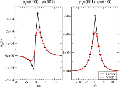
Figure 1: The amplitude $A_{\pi}(\tau)$ as a function of $\tau$ for momentum setups 1 (left) and 2 (right). The black (red) curves indicate the lattice (VMD) amplitudes.

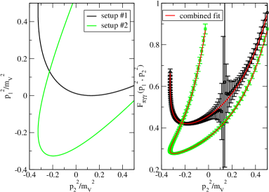
Figure 2: Left: Contour of $(p_{1}^{2},p_{2}^{2})$ rescaled by $1/M_{V}^{2}$ for our momentum setups. Right: $F_{\pi^{0}\gamma\gamma}(m_{\pi}^{2},p_{1}^{2},p_{2}^{2})$ as a function of $p_{2}^{2}/M_{V}^{2}$.

From the large $t_{1,2}-t_{\pi}$ behavior of $C_{\mu\nu}(t_{1},t_{2},t_{\pi})$, it is possible to extract the $\pi^{0}$-ground state. We define the amplitude $A_{\pi}$ as

$$A_{\pi}(\tau)\equiv\lim_{t-t_{\pi}\rightarrow\infty}C_{\mu\nu}(t_{1},t_{2},t_{\pi})/e^{-E_{\pi,\vec{q}}(t-t_{\pi})}\;,$$ (9)

with $\tau=t_{1}-t_{2}$ and $t=\textmd{min}\{t_{1},t_{2}\}$, and obtain $M_{\mu\nu}(p_{1},p_{2})$ by performing an integral

$$\frac{2E_{\pi,\vec{q}}}{\phi_{\pi}}\left(\int_{0}^{\infty}d\tau\;e^{\omega\tau}A_{\pi}(\tau)+\int_{-\infty}^{0}d\tau\;e^{(\omega-E_{\pi,\vec{q}})\tau}A_{\pi}(\tau)\right)\;.$$ (10)

The spatial momenta are assigned as $\vec{p}_{1}=\frac{2\pi}{L}(0,0,0)$, $\vec{q}=\frac{2\pi}{L}(0,0,1)$ (setup 1) and $\vec{p}_{1}=\frac{2\pi}{L}(0,0,1)$, $\vec{q}=\frac{2\pi}{L}(0,0,0)$ (setup 2). The resulting amplitudes $A_{\pi}(\tau)$ for these setups are shown by the black curves in Fig. 2. The amplitude $A_{\pi}^{\rm VMD}(\tau)$, constructed from the vector-meson-dominance (VMD) form factor ${\mathcal{F}}_{\pi^{0}\gamma\gamma}^{\rm VMD}(m_{\pi}^{2},p_{1}^{2},p_{2}^{2})=c_{V}G_{V}(p_{1}^{2})G_{V}(p_{2}^{2})$, with $G_{V}(p^{2})=M_{V}^{2}/(M_{V}^{2}-p^{2})$ the vector meson propagator and $c_{V}$ a constant is also plotted by red curves. We find that $A_{\pi}^{\rm VMD}(\tau)$ give a good approximation to the lattice data at large $|\tau|$ but fails to match them at small $|\tau|$. This is because no information of the vector-meson excited states are contained in ${\mathcal{F}}_{\pi^{0}\gamma\gamma}^{\rm VMD}(m_{\pi}^{2},p_{1}^{2},p_{2}^{2})$. Although the lattice data are truncated due to the finite time extent $T$, we are still able to perform the integral (10) from $-\infty$ to $+\infty$ since the $A_{\pi}(\tau)$ at the large $|\tau|$ is dominated by the lowest vector meson.

When performing the integral (10) we can tune the value of the photon energy $\omega$ continuously. As shown in the left panel of Fig. 2, a pair $(p_{1}^{2},p_{2}^{2})=(\omega^{2}-\vec{p}_{1}^{2},(E_{\pi,\vec{q}}-\omega)^{2}-(\vec{q}-\vec{p}_{1})^{2})$ forms a continuous contour on the $(p_{1}^{2},p_{2}^{2})$ plane for $p_{1,2}^{2}<M_{V}^{2}/2$. Evaluating ${\mathcal{F}}_{\pi^{0}\gamma\gamma}(m_{\pi}^{2},p_{1}^{2},p_{2}^{2})$ along this contour, we obtain the data plotted in the right panel of Fig. 2. We use the fit ansatz ${\mathcal{F}}_{\pi^{0}\gamma\gamma}(m_{\pi}^{2},p_{1}^{2},p_{2}^{2})=$

$$c_{V}G_{V}(p_{1}^{2})G_{V}(p_{2}^{2})+\sum_{m}c_{m}\left((p_{2}^{2})^{m}G_{V}(p_{1}^{2})+(p_{1}^{2})^{m}G_{V}(p_{2}^{2})\right)+\sum_{m,n}c_{m,n}(p_{1}^{2})^{m}(p_{2}^{2})^{n}\;,$$ (11)

which includes the contribution from the lowest vector meson through $G_{V}(p_{1,2}^{2})$ and the contribution from excited states as a polynomial of $p_{1,2}^{2}$. We perform the combined fit of the lattice data to Eq. (11) with four free parameters: $c_{V}$, $c_{0}$, $c_{0,0}$ and $c_{0,1}=c_{1,0}$. The contributions from the higher-order terms are not significant when compared to the statistical error and thus can be neglected. The fitting curves are shown in the right panel of Fig. 2. We find that the single formula (11) describes the data with different momentum setups. Using the resulting fit parameters and extrapolating ${\mathcal{F}}_{\pi^{0}\gamma\gamma}(m_{\pi}^{2},p_{1}^{2},p_{2}^{2})$ to the soft photon limit, we obtain the normalized form factors $F(m_{\pi}^{2},0,0)=(4\pi^{2}F_{\pi}){\mathcal{F}}_{\pi^{0}\gamma\gamma}(m_{\pi}^{2},0,0)$, which are plotted in the uppermost panel of Fig. 3.

$\begin{array}[]{c}\includegraphics[width=200.0pt,angle={0}]{before_correction-crop}\\ \includegraphics[width=200.0pt,angle={0}]{after_correction-crop}\end{array}$

Figure 3: $F(m_{\pi}^{2},0,0)$, $g_{V}$, $g_{V\pi\gamma}$, $F_{\pi}$ and FS corrected $F(m_{\pi}^{2},0,0)$ as a function of $m_{\pi}^{2}$ from top to bottom panels. In each panel, data with $(L/a,Q)=(16,0)$, $(24,0)$ and $(16,1)$ are plotted by the blue, red and green symbols, respectively. The yellow symbols indicate the Particle Data Group (PDG) [17] or PrimEx [6] experimental values for reference. The solid (dashed) curves show the result of the fit to the linear (quadratic) function. The dataset used in the fit is explained in the text.

Using the results of $F(m_{\pi}^{2},0,0)$ we analyze the various systematic effects including FS effects, fixed-topology effects, disconnected-diagram effects, higher-order effects in chiral extrapolation and possible discretization effects in the evaluation of Eq. (7). For more details of the analysis, we refer the readers to our recent publication [18].

Among the various systematic effects, the largest one is the conventional FS effect. As shown in Fig. 3, at $m_{\pi}\approx 290$ MeV we find that $F(m_{\pi}^{2},0,0)$ calculated at $L/a=16$ lattice is 27% less than the one at $L/a=24$. To qualitatively understand this FS effect, we insert the ground state into $\langle j_{\mu}j_{\nu}\pi^{0}\rangle$ and approximate this three-point correlation function with three hadronic matrix elements: $\langle j_{\mu}j_{\nu}\pi^{0}\rangle\rightarrow\langle\Omega|j_{\mu}|V,\varepsilon\rangle\langle V,\varepsilon|j_{\nu}|\pi^{0}\rangle\langle\pi^{0}|\pi^{0}|\Omega\rangle$. These matrix elements are related to the electromagnetic coupling $g_{V}$, the $V\pi\gamma$ coupling $g_{V\pi\gamma}$ and the pion decay constant $F_{\pi}$. In our calculation we do not observe significant FS effect in $M_{V}$ but find 8%, 7% and 9% shifts in $g_{V}$, $g_{V\pi\gamma}$ and $F_{\pi}$, respectively, from $L/a=16$ to 24, as shown in Fig. 3. These FS effects may accumulate in the three-point function. We estimate the FS corrections to $g_{V}$, $g_{V\pi\gamma}$ and $F_{\pi}$ by adding a correction term, $e^{-m_{\pi}L}$, into the linear fit form in the chiral extrapolation of each quantity or using NNLO chiral perturbation theory. We then combine the FS corrections to each quantity as an estimation of the total FS correction to $F(m_{\pi}^{2},0,0)$. As shown in the lowest panel of Fig. 3 the FS corrected $F(m_{\pi}^{2},0,0)$ at $L/a=16$ agrees with those at $L/a=24$.

We use two methods of treating the FS effects: 1. We use the uncorrected $F(m_{\pi}^{2},0,0)$ with $m_{\pi}L>4$ to perform the chiral extrapolation. Namely, we exclude the $L/a=16$ data points at two lowest pion masses. A linear function in $m_{\pi}^{2}$ is used as an fit ansatz. 2. We use the FS corrected data of all ensembles to perform a linear extrapolation. The difference between the results from the two methods is considered as a systematic error.

We quote our results for $F(0,0,0)$ and $\Gamma_{\pi^{0}\gamma\gamma}$ in the isospin symmetric limit as $F(0,0,0)=1.009(22)(29)$ and $\Gamma_{\pi^{0}\gamma\gamma}=7.83(31)(49)$ eV, where the first error is statistical and the second one is systematic. Our results reproduce the predication of the ABJ anomaly $F(0,0,0)=1$ and agree with the PrimEx measurement $\Gamma_{\pi^{0}\gamma\gamma}=7.82(22)$ eV [6]. For future improvements, isospin breaking effects due to the light quark mass difference need to be included.

Numerical simulations are performed on the Hitachi SR16000 at Yukawa Institute of Theoretical Physics and at High Energy Accelerator Research Organization under a support of its Large Scale Simulation Program (No. 11-05). This work is supported in part by the Grant-in-Aid of the Japanese Ministry of Education (No.21674002, 21684013), the Grant-in-Aid for Scientific Research on Innovative Areas (No. 2004: 20105001, 20105002, 20105003, 20105005, 23105710), and SPIRE (Strategic Program for Innovative Research).

References

- [1] D. Sutherland, Nucl.Phys. B2, 433 (1967).
- [2] M. Veltman, Proc. Roy. Soc. A301, 107 (1967).
- [3] S. L. Adler, Phys. Rev. 177, 2426 (1969).
- [4] J. S. Bell and R. Jackiw, Nuovo Cim. A60, 47 (1969).
- [5] S. L. Adler and W. A. Bardeen, Phys. Rev. 182, 1517 (1969).
- [6] PrimEx, I. Larin et al., Phys. Rev. Lett. 106, 162303 (2011), 1009.1681.
- [7] L. H. Karsten and J. Smit, Nucl.Phys. B183, 103 (1981).
- [8] M. Luscher, Phys.Lett. B428, 342 (1998), hep-lat/9802011.
- [9] K. Fujikawa and M. Ishibashi, Nucl.Phys. B587, 419 (2000), hep-lat/0005003.
- [10] X. D. Ji and C. W. Jung, Phys. Rev. Lett. 86, 208 (2001), hep-lat/0101014.
- [11] J. J. Dudek and R. G. Edwards, Phys. Rev. Lett. 97, 172001 (2006), hep-ph/0607140.
- [12] S. D. Cohen, H. W. Lin, J. Dudek, and R. G. Edwards, PoS LATTICE2008, 159 (2008), 0810.5550.
- [13] JLQCD and TWQCD Collaborations, H. Matsufuru et al., PoS LATTICE2008, 077 (2008).
- [14] JLQCD and TWQCD Collaborations, J. Noaki et al., PoS LATTICE2010, 117 (2010).
- [15] S. Aoki, H. Fukaya, S. Hashimoto, and T. Onogi, Phys. Rev. D76, 054508 (2007), 0707.0396.
- [16] J. Noaki et al., Phys. Rev. D81, 034502 (2010), 0907.2751.
- [17] Particle Data Group, K. Nakamura et al., J. Phys. G37, 075021 (2010).
- [18] X. Feng et al., accepted by Phys. Rev. Lett. (2012), 1206.1375.