Random Utility Theory for Social Choice

Abstract

Random utility theory models an agent’s preferences on alternatives by drawing a real-valued score on each alternative (typically independently) from a parameterized distribution, and then ranking the alternatives according to scores. A special case that has received significant attention is the Plackett-Luce model, for which fast inference methods for maximum likelihood estimators are available. This paper develops conditions on general random utility models that enable fast inference within a Bayesian framework through MC-EM, providing concave log-likelihood functions and bounded sets of global maxima solutions. Results on both real-world and simulated data provide support for the scalability of the approach and capability for model selection among general random utility models including Plackett-Luce.

1 Introduction

Problems of learning with rank-based error metrics [Liu11:Learning] and the adoption of learning for the purpose of rank aggregation in social choice [Conitzer05:Common, Conitzer09:Preference, Xia10:Aggregating, Xia11:Maximum, Roos11:How, Procaccia12:Maximum] are gaining in prominence in recent years. In part, this is due to the explosion of socio-economic platforms, where opinions of users need to be aggregated; e.g., judges in crowd-sourcing contests, ranking of movies or user-generated content.

In the problem of social choice, users submit ordinal preferences consisting of partial or total ranks on the alternatives and a single rank order must be selected to be representative of the reports. Since Condorcet [Condorcet1785:Essai], one approach to this problem is to formulate social choice as the problem of estimating a true underlying world state (e.g., a true quality ranking of alternatives), where the individual reports are viewed as noisy data in regard to the true state. In this way, social choice can be framed as a problem of inference.

In particular, Condorcet assumed the existence of a true ranking over alternatives, with a voter’s preference between any pair of alternatives $a,b$ generated to agree with the true ranking with probability $p>1/2$ and disagree otherwise. Condorcet proposed to choose as the outcome of social choice the ranking that maximizes the likelihood of observing the voters’ preferences. Later, Kemeny’s rule was shown to provide the maximum likelihood estimator (MLE) for this model [Young95:Optimal].

But Condorcet’s probabilistic model assumes identical and independent distributions on pairwise comparisons. This ignores the strength in agents’ preferences (the same probability $p$ is adopted for all pairwise comparisons), and allows for cyclic preferences. In addition, computing the winner through the Kemeny rule is $\Theta_{2}^{P}$-complete [Hemaspaandra05:Complexity].

To overcome the first criticism, a more recent literature adopts the random utility model (RUM) from economics [Thurstone27:Law]. Consider $\mathcal{C}=\{c_{1},..,c_{m}\}$ alternatives. In RUM, there is a ground truth utility (or score) associated with each alternative. These are real-valued parameters, denoted by $\vec{\theta}=(\theta_{1},\ldots,\theta_{m})$. Given this, an agent independently samples a random utility ($X_{j}$) for each alternative $c_{j}$ with conditional distribution $\mu_{j}(\cdot|\theta_{j})$.

Usually $\theta_{j}$ is the mean of $\mu_{j}(\cdot|\theta_{j})$. Let $\pi$ denote a permutation of $\{1,\ldots,m\}$, which naturally corresponds to a linear order: $[c_{\pi(1)}\succ c_{\pi(2)}\succ\cdots\succ c_{\pi(m)}]$. Slightly abusing notation, we also use $\pi$ to denote this linear order. Random utility $(X_{1},\ldots,X_{m})$ generates a distribution on preference orders, as

$$\text{Pr}(\pi\ |\ \vec{\theta})=\text{Pr}(X_{\pi(1)}>X_{\pi(2)}>\ldots>X_{\pi(m)})$$ (1)

The generative process is illustrated in Figure 1.

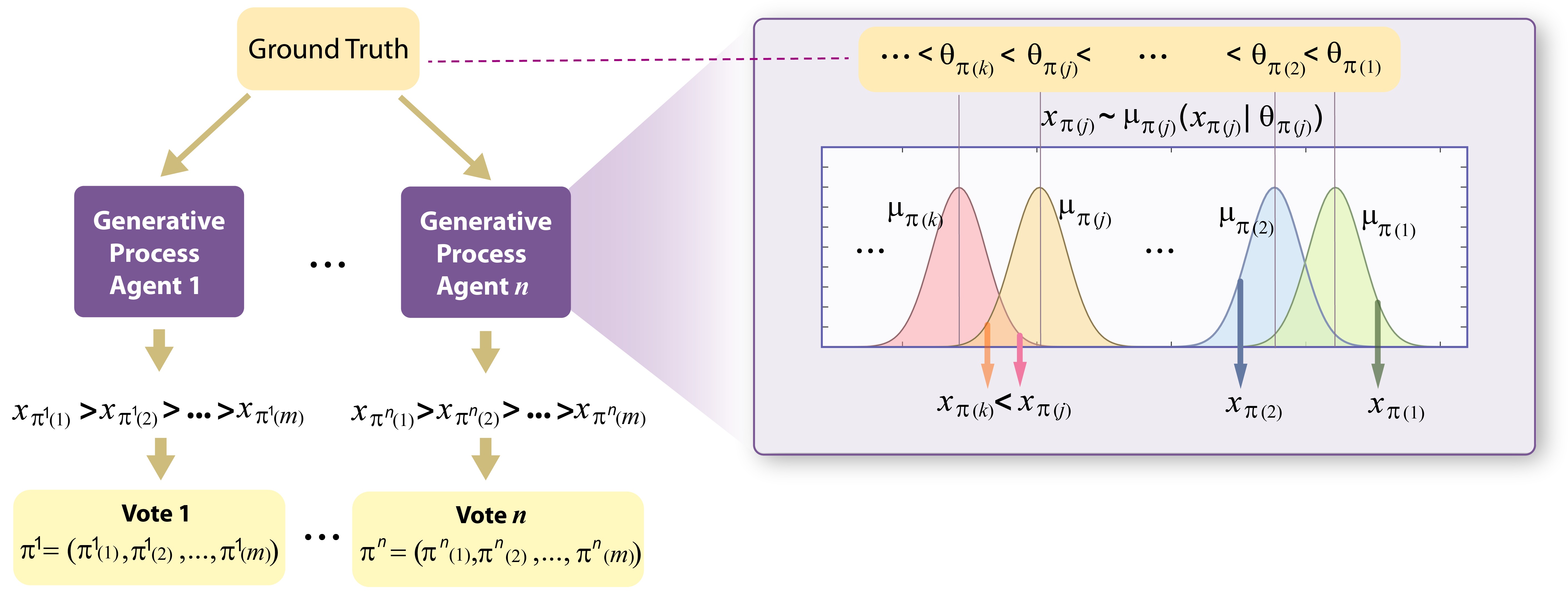
Figure 1: The generative process for RUMs.

Adopting RUMs rules out cyclic preferences, because each agent’s outcome corresponds to an order on real numbers, and it also captures the strength of preference, and thus overcomes the second criticism, by assigning a different parameter ($\theta_{j}$) to each alternative.

A popular RUM is Plackett-Luce (P-L) [Luce59:Individual, Plackett75:Analysis], where the random utility terms are generated according to Gumbel distributions with fixed shape parameter [Block60:Random, Yellott77:Relationship]. For P-L, the likelihood function has a simple analytical solution, making MLE inference tractable. P-L has been extensively applied in econometrics [McFadden74:Conditional, Berry95:Automobile], and more recently in machine learning and information retrieval (see [Liu11:Learning] for an overview). Efficient methods of EM inference [Hunter04:MM, Caron12:Efficient], and more recently expectation propagation [Guiver09:Bayesian], have been developed for P-L and its variants.

In application to social choice, the P-L model has been used to analyze political elections [Gormley09:Grade]. EM algorithm has also been used to learn the Mallows model, which is closely related to the Condorcet’s probabilistic model [Lu11:Learning].

Although P-L overcomes the two difficulties of the Condorcet-Kemeny approach, it is still quite restricted, by assuming that the random utility terms are distributed as Gumbel, with each alternative is characterized by one parameter, which is the mean of its corresponding distribution. In fact, little is known about inference in RUMs beyond P-L. Specifically, we are not aware of either an analytical solution or an efficient algorithm for MLE inference for one of the most natural models proposed by Thurstone [Thurstone27:Law], where each $X_{j}$ is normally distributed.

1.1 Our Contributions

In this paper we focus on RUMs in which the random utilities are independently generated with respect to distributions in the exponential family (EF) [Morris12:Natural]. This extends the P-L model, since the Gumbel distribution with fixed shape parameters belonging to the EF. Our main theoretical contributions are Theorem 1 and Theorem 2, which propose conditions such that the log-likelihood function is concave and the set of global maxima solutions is bounded for the location family, which are RUMs where the shape of each distribution $\mu_{j}$ is fixed and the only latent variables are the locations, i.e., the means of $\mu_{j}$’s. These results hold for existing special cases, such as the P-L model, and many other RUMs, for example the ones where each $\mu_{j}$ is chosen from Normal, Gumbel, Laplace and Cauchy.

We also propose a novel application of MC-EM. We treat the random utilities ($\vec{X}$) as latent variables, and adopt the Expectation Maximization (EM) method to estimate parameters $\vec{\theta}$. The E-step for this problem is not analytically tractable, and for this we adopt a Monte Carlo approximation. We establish through experiments that the Monte-Carlo error in the E-step is controllable and does not affect inference, as long as numerical parameterizations are chosen carefully. In addition, for the E-step we suggest a parallelization over the agents and alternatives and a Rao-Blackwellized method, which further increases the scalability of our method.

We generally assume that the data provides total orders on alternatives from voters, but comment on how to extend the method and theory to the case where the input preferences are partial orders.

We evaluate our approach on synthetic data as well as two real-world datasets, a public election dataset and one involving rank preferences on sushi. The experimental results suggest that the approach is scalable despite providing significantly improved modeling flexibility over existing approaches.

For the two real-world datasets we have studied, we compare RUMs with normal distributions and P-L in terms of four criteria: log-likelihood, predictive log-likelihood, Akaike information criterion (AIC), and Bayesian information criterion (BIC). We observe that when the amount of data is not too small, RUMs with normal distributions fit better than P-L. Specifically, for the log-likelihood, predictive log-likelihood, and AIC criteria, RUMs with normal distributions outperform P-L with 95% confidence in both datasets.

2 RUMs and Exponential Families

In social choice, each agent $i\in\{1,\ldots,n\}$ has a strict preference order on alternatives. This provides the data for an inferential approach to social choice. In particular. let $L(\mathcal{C})$ denote the set of all linear orders on $\mathcal{C}$. Then, a preference-profile, $D$, is a set of $n$ preference orders, one from each agent, so that $D\in L(\mathcal{C})^{n}$.

A voting rule $r$ is a mapping that assigns to each preference-profile a set of winning rankings, $r:L(\mathcal{C})^{n}\mapsto(2^{L(\mathcal{C})}\setminus\emptyset)$. In particular, in the case of ties the set of winning rankings may include more than a singleton ranking. In the maximum likelihood (MLE) approach to social choice, the preference profile is viewed as data, $D=\{\pi^{1},\ldots,\pi^{n}\}$.

Given this, the probability (likelihood) of the data given ground truth $\vec{\theta}$ (and for a particular $\vec{\mu}$) is $\Pr(D\ |\ \vec{\theta})=\prod^{n}_{i=1}\Pr(\pi^{i}\ |\ \vec{\theta}),$ where,

$$\!\!P(\pi|\vec{\theta})\!=\!\!\!\int^{\infty}_{x_{\pi(n)}=-\infty}\int^{\infty}_{x_{\pi(n-1)}=x_{\pi(n)}}\!\!\!..\int^{\infty}_{x_{\pi(1)}=x_{\pi(2)}}\!\!\!\!\!\!\!\!\mu_{\pi(n)}(x_{\pi(n)})..\mu_{\pi(1)}(x_{\pi(1)})dx_{\pi(1)}dx_{\pi(2)}..dx_{\pi(n)}$$ (2)

The MLE approach to social choice selects as the winning ranking that which corresponds to the $\vec{\theta}$ that maximizes $\Pr(D\ |\ \vec{\theta})$. In the case of multiple parameters that maximize the likelihood then the MLE approach returns a set of rankings, one ranking corresponding to each parameterization.

In this paper, we focus on probabilistic models where each $\mu_{j}$ belongs to the exponential family (EF). The density function for each $\mu$ in EF has the following format:

$$\text{Pr}(X=x) =\mu(x)=e^{\eta(\theta)T(x)-A(\theta)+B(x)},$$ (3)

where $\eta(\cdot)$ and $A(\cdot)$ are functions of $\theta$, $B(\cdot)$ is a function of $x$, and $T(x)$ denotes the sufficient statistics for $x$, which could be multidimensional.

Example 1 (Plackett-Luce as an RUM [Block60:Random]).

In the RUM, let $\mu_{j}$’s be Gumbel distributions. That is, for alternative $j\in\{1,\ldots,m\}$ we have $\mu_{j}(x_{j}|\theta_{j})=e^{-(x_{j}-\theta_{j})}e^{-e^{-(x_{j}-\theta_{j})}}$. Then, we have: $\text{Pr}(\pi\ |\ \vec{\lambda})=\text{Pr}(x_{\pi(1)}>x_{\pi(2)}>..>x_{\pi(m)})=\prod^{m}_{j=1}{\lambda_{\pi(j)}\over\sum^{m}_{j^{\prime}=j}\lambda_{\pi(j^{\prime})}}$ , where $\eta({\theta_{j}})=\lambda_{j}=e^{\theta_{j}}$, $T(x_{j})=-e^{-x_{j}}$, $B(x_{j})=-x_{j}$ and $A(\theta_{j})=-\theta_{j}$.This gives us the Plackett-Luce model.

3 Global Optimality and Log-Concavity

In this section, we provide a condition on distributions that guarantees that the likelihood function (2) is log-concave in parameters $\vec{\theta}$. We also provide a condition under which the set of MLE solutions is bounded when any one latent parameter is fixed. Together, this guarantees the convergence of our MC-EM approach to a global mode with an accurate enough E-step. We focus on the location family, which is a subset of RUMs where the shapes of all $\mu_{j}$’s are fixed, and the only parameters are the means of the distributions. For the location family, we can write $X_{j}=\theta_{j}+\zeta_{j}$, where $X_{j}\sim\mu_{j}(\cdot|\theta_{j})$ and $\zeta_{j}=X_{j}-\theta_{j}$ is a random variable whose mean is $0$ and models an agent’s subjective noise. The random variables $\zeta_{j}$’s do not need to be identically distributed for all alternatives $j$; e.g., they can be normal with different fixed variances.

We focus on computing solutions ($\vec{\theta}$) to maximize the log-likelihood function,

$$l(\vec{\theta};D)=\sum^{n}_{i=1}\log\Pr(\pi^{i}\ |\ {\vec{\theta}})$$ (4)

Theorem 1.

For the location family, if for every $j\leq m$ the probability density function for $\zeta_{j}$ is log-concave, then $l(\vec{\theta};D)$ is concave.

Proof sketch: The theorem is proved by applying the following lemma, which is Theorem 9 in [Prekopa80:Logarithmic].

Lemma 1.

Suppose $g_{1}(\vec{\theta},\vec{\zeta}),...,g_{R}(\vec{\theta},\vec{\zeta})$ are concave functions in $\mathbb{R}^{2m}$ where $\vec{\theta}$ is the vector of $m$ parameters and $\vec{\zeta}$ is a vector of $m$ real numbers that are generated according to a distribution whose pdf is logarithmic concave in $\mathbb{R}^{m}$. Then the following function is log-concave in $\mathbb{R}^{m}$.

$$L_{i}(\vec{\theta},G)=\Pr(g_{1}(\vec{\theta},\vec{\zeta})\geq 0,...,g_{R}(\vec{\theta},\vec{\zeta})\geq 0),\ \ \vec{\theta}\in\mathbb{R}^{m}$$ (5)

To apply Lemma 1, we define a set $G^{i}$ of function $g^{i}$’s that is equivalent to an order $\pi^{i}$ in the sense of inequalities implied by RUM for $\pi^{i}$ and $G^{i}$ (the joint probability in (5) for $G^{i}$ to be the same as the probity of $\pi^{i}$ in RUM with parameters $\vec{\theta}$). Suppose $g^{i}_{r}(\vec{\theta},\vec{\zeta})=\theta_{\pi^{i}(r)}+\zeta^{i}_{\pi^{i}(r)}-\theta_{\pi^{i}{(r+1)}}-\zeta^{i}_{{\pi^{i}({r+1})}}$ for $r=1,..,m-1$.

Then considering that the length of order $\pi^{i}$ is $R+1$, we have:

$$L_{i}(\vec{\theta},\pi^{i})=L_{i}(\vec{\theta},G^{i})=\Pr(g^{i}_{1}(\vec{\theta},\vec{\zeta})\geq 0,...,g^{i}_{R}(\vec{\theta},\vec{\zeta})\geq 0),\ \ \vec{\theta}\in\mathbb{R}^{m}$$ (6)

This is because $g^{i}_{r}(\vec{\theta},\vec{\zeta})\geq 0$ is equivalent to that in $\pi^{i}$ alternative $\pi^{i}(r)$ is preferred to alternative $\pi^{i}(r+1)$ in the RUM sense.

To see how this extends to the case where preferences are specified as partial orders, we consider in particular an interpretation where an agent’s report for the ranking of $m_{i}$ alternatives implies that all other alternatives are worse for the agent, in some undefined order. Given this, define $g^{i}_{r}(\vec{\theta},\vec{\zeta})=\theta_{\pi^{i}(r)}+\zeta^{i}_{\pi^{i}(r)}-\theta_{\pi^{i}{(r+1)}}-\zeta^{i}_{{\pi^{i}({r+1})}}$ for $r=1,..,m_{i}-1$ and $g^{i}_{r}(\vec{\theta},\vec{\zeta})=\theta_{\pi^{i}(m_{i})}+\zeta^{i}_{\pi^{i}(m_{i})}-\theta_{\pi^{i}{(r+1)}}-\zeta^{i}_{{\pi^{i}({r+1})}}$ for $r=m_{i},..,m-1$. Considering that $g^{i}_{r}(\cdot)$s are linear (hence, concave) and using log concavity of the distributions of $\vec{\zeta^{i}}=(\zeta^{i}_{1},\zeta^{i}_{2},..,\zeta^{i}_{m})$’s, we can apply Lemma 1 and prove log-concavity of the likelihood function. $\Box$

It is not hard to verify that pdfs for normal and Gumbel are log-concave under reasonable conditions for their parameters, made explicit in the following corollary.

Corollary 1.

For the location family where each $\zeta_{j}$ is a normal distribution with mean zero and with fixed variance, or Gumbel distribution with mean zeros and fixed shape parameter, $l(\vec{\theta};D)$ is concave. Specifically, the log-likelihood function for P-L is concave.

The concavity of log-likelihood of P-L has been proved [Ford57:Solution] using a different technique. Using Fact 3.5. in [Proschan89:Log], the set of global maxima solutions to the likelihood function, denoted by $S_{D}$, is convex since the likelihood function is log-concave. However, we also need that $S_{D}$ is bounded, and would further like that it provides one unique order as the estimation for the ground truth.

For P-L, Ford, Jr. [Ford57:Solution] proposed the following necessary and sufficient condition for the set of global maxima solutions to be bounded (more precisely, unique) when $\sum_{j=1}^{m}e^{\theta_{j}}=1$.

Condition 1.

Given the data $D$, in every partition of the alternatives $\mathcal{C}$ into two nonempty subsets $\mathcal{C}_{1}\cup\mathcal{C}_{2}$, there exists $c_{1}\in\mathcal{C}_{1}$ and $c_{2}\in\mathcal{C}_{2}$ such that there is at least one ranking in $D$ where $c_{1}\succ c_{2}$.

We next show that Condition 1 is also a necessary and sufficient condition for the set of global maxima solutions $S_{D}$ to be bounded in location families, when we set one of the values $\theta_{j}$ to be $0$ (w.l.o.g., let $\theta_{1}=0$). If we do not bound any parameter, then $S_{D}$ is unbounded, because for any $\vec{\theta}$, any $D$, and any number $s\in\mathbb{R}$, $l(\vec{\theta};D)=l(\vec{\theta}+s;D)$.

Theorem 2.

Suppose we fix $\theta_{1}=0$. Then, the set $S_{D}$ of global maxima solutions to $l(\theta;D)$ is bounded if and only if the data $D$ satisfies Condition 1.

Proof sketch:

If Condition 1 does not hold, then $S_{D}$ is unbounded because the parameters for all alternatives in $C_{1}$ can be increased simultaneously to improve the log-likelihood. For sufficiency, we first present the following lemma.

Lemma 2.

If alternative $j$ is preferred to alternative $j^{\prime}$ in at least in one ranking then the difference of their mean parameters $\theta_{j^{\prime}}-\theta_{j}$ is bounded from above ($\exists Q\ where\ \theta_{j^{\prime}}-\theta_{j}<Q$) for all the $\vec{\theta}$ that maximize the likelihood function.

Proof.

Suppose that $j\succ j^{\prime}$ in rank $i$, then for any $\vec{\theta}\in\mathbb{R}^{m}$:

$$L_{i}(\vec{\theta},\pi^{i})=L_{i}(\vec{\theta},G^{i})=\Pr(g_{1}(\vec{\theta},\vec{\zeta})\geq 0,...,g_{R}(\vec{\theta},\vec{\zeta})\geq 0)$$

$$\leq \Pr(g_{\pi^{i}(r)}(\vec{\theta},\vec{\zeta})\geq 0,g_{\pi^{i}(r+1)}(\vec{\theta},\vec{\zeta})\geq 0,\ldots,g_{\pi^{i}(r^{\prime})}(\vec{\theta},\vec{\zeta})\geq 0)\leq\Pr(\zeta_{j}-\zeta_{j^{\prime}}\geq\theta_{j^{\prime}}-\theta_{j}),$$ (7)

where $j=\pi^{i}(r)$ and $j^{\prime}=\pi^{i}(r^{\prime})$.

Let $K=l(\vec{0};D)$. Since the log-likelihood is always smaller than $0$, it follows that for any $\vec{\theta}\in S_{D}$ and any $i\leq n$, $L_{i}(\vec{\theta};\pi^{i})\geq K$.

Hence, $\Pr(\zeta_{j}-\zeta_{j^{\prime}}\geq\theta_{j^{\prime}}-\theta_{j})\geq K$.

Therefore, there exists $K^{\prime}$ such that $\theta_{j^{\prime}}-\theta_{j}<K^{\prime}$, where $K^{\prime}$ depends on the fixed $\zeta_{j^{\prime}}$ and $\zeta_{j}$.

Now consider a directed graph $G_{D}$, where the nodes are the alternatives, and there is an edge between $c_{j}$ to $c_{j^{\prime}}$ if in at least one ranking $c_{j}\succ c_{j^{\prime}}$. By Condition 1, for any pair $j\neq j^{\prime}$, there is a path from $c_{j}$ to $c_{j^{\prime}}$ (and conversely, a path from $c_{j^{\prime}}$ to $c_{j}$). To see this, consider building a path between $j$ and $j^{\prime}$ by starting from a partition with ${\mathcal{C}}_{1}=\{j\}$ and following an edge from $j$ to $j_{1}$ in the graph where $j_{1}$ is an alternatives in ${\mathcal{C}}_{2}$ for which there must be such an edge, by Condition 1. Consider the partition with ${\mathcal{C}}_{1}=\{j,j_{1}\}$, and repeat until an edge can be followed to vertex $j^{\prime}\in{\mathcal{C}}_{2}$. It follows from Lemma 2 that for any $\vec{\theta}\in S_{D}$ we have $|\theta_{j}-\theta_{j^{\prime}}|<Qm$, using the telescopic sum of bounded values of the difference of mean parameters along the edges of the path, since the length of the path is no more than $m$ (and tracing the path from $j$ to $j^{\prime}$ and $j^{\prime}$ to $j$), meaning that $S_{D}$ is bounded. $\Box$

Now that we have the log concavity and bounded property, we need to declare conditions under which the bounded convex space of estimated parameters corresponds to a unique order. The next theorem provides a necessary and sufficient condition for all global maxima to correspond to the same order on alternatives. Suppose that we order the alternatives based on estimated $\theta$’s (meaning that $c_{j}$ is ranked higher than $c_{j^{\prime}}$ iff $\theta_{j}>\theta_{j^{\prime}}$).

Theorem 3.

The order over parameters is strict and is the same across all $\vec{\theta}\in S_{D}$ if, for all $\vec{\theta}\in S_{D}$ and all alternatives $j\neq j^{\prime}$, $\theta_{j}\neq\theta_{j^{\prime}}$.

Proof.

Suppose for the sake of contradiction there exist two maxima, $\vec{\theta},\vec{\theta}^{*}\in S_{D}$ and a pair of alternatives $j\neq j^{\prime}$ such that $\theta_{j}>\theta_{j^{\prime}}$ and $\theta^{*}_{j^{\prime}}>\theta_{j}^{*}$. Then, there exists an $\alpha<1$ such that the $j$th and $j^{\prime}$th components of $\alpha\vec{\theta}+(1-\alpha)\vec{\theta}^{*}$ are equal, which contradicts the assumption.

Hence, if there is never a tie in the scores in any $\vec{\theta}\in S_{D}$, then any vector in $S_{D}$ will reveal the unique order.

4 Monte Carlo EM for Parameter Estimation

In this section, we propose an MC-EM algorithm for MLE inference for RUMs where every $\mu_{j}$ belongs to the EF.

The EM algorithm determines the MLE parameters $\vec{\theta}$ iteratively, and proceeds as follows. In each iteration $t+1$, given parameters $\vec{\theta}^{t}$ from the previous iteration, the algorithm is composed of an E-step and an M-step. For the E-step, for any given $\vec{\theta}=(\theta_{1},\ldots,\theta_{m})$, we compute the conditional expectation of the complete-data log-likelihood (latent variables $\vec{x}$ and data $D$), where the latent variables $\vec{x}$ are distributed according to data $D$ and parameters $\vec{\theta}^{t}$ from the last iteration.

For the M-step, we optimize $\vec{\theta}$ to maximize the expected log-likelihood computed in the E-step, and use it as the input $\vec{\theta}^{t+1}$ for the next iteration:

$$\mbox{E-Step :}\ \ \ Q(\vec{\theta},\vec{\theta}^{t})=E_{\vec{X}}\left\{\log\prod_{i=1}^{n}\Pr(\vec{x}^{i},\pi^{i}\ |\ \vec{\theta})\ |\ D,\vec{\theta}^{t}\right\}$$

$$\mbox{M-step :}\ \ \ \vec{\theta}^{t+1}\in\arg\max_{\vec{\theta}}Q(\vec{\theta},\vec{\theta}^{t})$$

4.1 Monte Carlo E-step by Gibbs sampler

The E-step can be simplified using (3) as follows:

$$E_{\vec{X}}\{\log\prod_{i=1}^{n}\Pr(\vec{x}^{i},\pi^{i}\ |\ \vec{\theta})\ |\ {D,\vec{\theta}^{t}}\}=E_{\vec{X}}\{\log\prod_{i=1}^{n}\Pr(\vec{x}^{i}|\ \vec{\theta})\Pr(\pi^{i}|\vec{x}^{i})\ |\ {D,\vec{\theta}^{t}}\}$$

$$=\sum_{i=1}^{n}\sum_{j=1}^{m}E_{X^{i}_{j}}\{\log\mu_{j}(x^{i}_{j}|\theta_{j})\ |\ \pi^{i},\vec{\theta}^{t}\}=\sum_{i=1}^{n}\sum_{j=1}^{m}(\eta(\theta_{j})E_{X^{i}_{j}}\{T(x^{i}_{j})\ |\ \pi^{i},\vec{\theta}^{t}\}-A(\theta_{j})+W,$$

where $W=E_{X^{i}_{j}}\{B(x^{i}_{j})\ |\ \pi^{i},\vec{\theta}^{t}\}$ only depends on $\vec{\theta}_{t}$ and $D$ (not on $\vec{\theta}$), which means that it can be treated as a constant in the M-step. Hence, in the E-step we only need to compute $S^{i,t+1}_{j}=E_{X_{j}^{i}}\{T(x^{i}_{j})\ |\ \pi^{i},\vec{\theta}^{t}\}$ where $T(x^{i}_{j})$ is the sufficient statistic for the parameter $\theta_{j}$ in the model. We are not aware of an analytical solution for $E_{X^{i}_{j}}\{T(x^{i}_{j})\ |\ \pi^{i},\vec{\theta}^{t}\}$. However, we can use a Monte Carlo approximation, which involves sampling $\vec{x}^{i}$ from the distribution $\Pr(\vec{x}^{i}\ |\ \pi^{i},\vec{\theta^{t}})$ using a Gibbs sampler, and then approximates $S^{i,t+1}_{j}$ by ${1\over N}\sum^{N}_{k=1}T(x^{i,k}_{j})$ where $N$ is the number of samples in the Gibbs sampler.

In each step of our Gibbs sampler for voter $i$, we randomly choose a position $j$ in $\pi^{i}$ and sample $x_{\pi^{i}(j)}^{i}$ according to a TruncatedEF distribution $\Pr(\cdot|\ x_{\pi^{i}(-j)},\vec{\theta^{t}},\pi^{i})$, where $\ x_{\pi^{i}(-j)}=(\ x_{\pi^{i}(1)},\ldots,\ x_{\pi^{i}(j-1)},\ x_{\pi^{i}(j+1)},\ldots,\ x_{\pi^{i}(m)})$. The TruncatedEF is obtained by truncating the tails of $\mu_{\pi^{i}(j)}(\cdot|\theta^{t}_{\pi^{i}(j)})$ at $x_{\pi^{i}(j-1)}$ and $x_{\pi^{i}(j+1)}$, respectively. For example, a truncated normal distribution is illustrated in Figure 2.

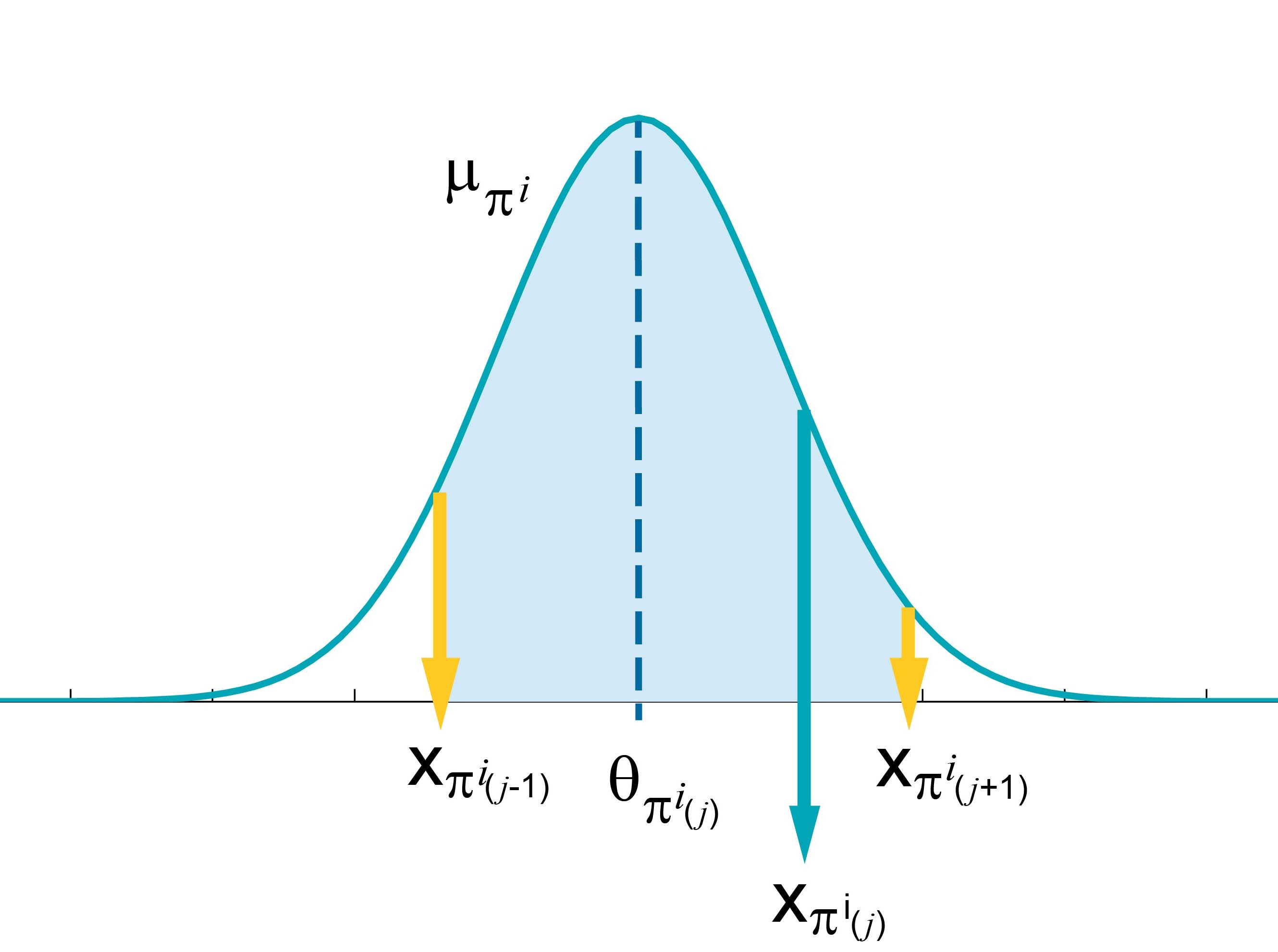
Figure 2: A truncated normal distribution.

Rao-Blackwellized: To further improve the Gibbs sampler, we use Rao-Blackwellized [Brooks11:Handbook] estimation using $E\{T(x^{i,k}_{j})\ |\ x^{i,k}_{-j},\pi^{i},\vec{\theta}^{t}\}$ instead of the sample $x^{i,k}_{j}$, where $x^{i,k}_{-j}$ is all of $\vec{x}^{i,k}$ except for $x^{i,k}_{j}$. Finally, we estimate $E\{T(x^{i,k}_{j})\ |\ x^{i,k}_{-j},\pi^{i},\vec{\theta}^{t}\}$ in each step of the Gibbs sampler using $M$ samples as $S_{j}^{i,t+1}\simeq{1\over N}\sum^{N}_{k=1}E\{T(x^{i,k}_{j})\ |\ x^{k}_{-j},\pi^{i},\vec{\theta}^{t}\}\simeq{1\over NM}\sum^{N}_{k=1}\sum^{M}_{l=1}T(x^{i^{l},k}_{j}),$ where $x^{i^{l},k}_{j}\sim\Pr(x^{i^{l},k}_{j}\ |\ x^{i,k}_{-j},\pi^{i},\vec{\theta})$. Rao-Blackwellization reduces the variance of the estimator because of conditioning and expectation in $E\{T(x^{i,k}_{j})\ |\ x^{i,k}_{-j},\pi^{i},\vec{\theta}^{t}\}$.