Towards Scalable Parallel-in-Time Turbulent Flow Simulations

Abstract

We present a reformulation of unsteady turbulent flow simulations. The initial condition is relaxed and information is allowed to propagate both forward and backward in time. Simulations of chaotic dynamical systems with this reformulation can be proven to be well-conditioned time domain boundary value problems. The reformulation can enable scalable parallel-in-time simulation of turbulent flows.

I Need for space-time parallelism

The use of computational fluid dynamics (CFD) in science and engineering can be categorized into Analysis and Design. A CFD Analysis performs a simulation on a set of manually picked parameter values. The flow field is then inspected to gain understanding of the flow physics. Scientific and engineering decisions are then made based on understanding of the flow field. Analysis based on high fidelity turbulent flow simulations, particular Large Eddy Simulations, is a rapidly growing practice in complex engineering applications Sagaut (2001) Pitsch (2006).

CFD based Design goes beyond just performing individual simulations, towards sensitivity analysis, optimization, control, uncertainty quantification and data based inference. Design is enabled by Analysis capabilities, but often requires more rapid turnaround. For example, an engineer designer or an optimization software needs to perform a series of simulations, modifying the geometry based on previous simulation results. Each simulation must complete within at most a few hours in an industrial design environment. Most current practices of design use steady state CFD solvers, employing RANS (Reynolds Averaged Navier-Stokes) models for turbulent flows. Design using high fidelity, unsteady turbulent flow simulations has been investigated in academiaMarsden et al. (2007). Despite their great potential, high fidelity design is infeasible in an industrial setting because each simulation typically takes days to weeks.

Figure 1: Exponential increase of high performance computing power, primarily sustained by increased parallelism in the past decade. Data originate from top500.org. GFLOPS, TFLOPS, PFLOPS and EFLOPS represent $10^{9}$, $10^{12}$, $10^{15}$ and $10^{18}$ FLoating point Operations Per Second, respectively.

The inability of performing high fidelity turbulent flow simulations in short turnaround time is a barrier to the game-changing technology of high fidelity CFD-based design. Nevertheless, development in High Performance Computing (HPC), as shown in Figure 1, promises to delivery in about ten years computing hardware a thousand times faster than those available today. This will be achieved through extreme scale parallelization of light weight, communication constrained cores Ruelle (1997). A 2008 study developed a straw man extreme scale system that could deliver $10^{18}$ FLOPS by combining about 166 million cores Kogge et al. (2008) Amarasinghe et al. (2009). CFD simulations running on a million cores can be as common in a decade as those running on a thousand cores today.

Will the projected thousand-fold increase in the number of computing cores lead to a thousand-fold decrease in turnaround time of high fidelity turbulent flow simulations? If the answer is yes, then the same LES that takes a week to complete on today’s systems would only take about 10 minutes in 2022. High fidelity CFD-based design in an industrial setting would then be a reality.

Figure 2: Typical LES in complex geometryMoin (2002) suffers from decreased parallel efficiency when the number of gridpoints per core is less than 10,000. The upward triangles, circles, downward triangles and squares represent meshes of 2M, 1M, 216k and 64k grid points, respectively.

The answer to this question hinges on development of more efficient, scalable and resilient parallel simulation paradigm. Current unsteady flow solvers are typically parallel only in space. Each core handles the flow field in a spatial subdomain. All cores advance simultaneously in time, and data is transferred at subdomain boundaries at each time step. This current simulation paradigm can achieve good parallel scaling when the number of grid points per core is large. However, Figure 2 shows that parallel efficiency quickly deteriorates as the number of grid points per core decreases below a few thousand. This limit is due to limited inter-core data transfer rate, a bottleneck expected to remain or worsen in the next generation HPC hardware. Therefore, it would be inefficient to run a simulation with a few million grid points on a million next-generation computing cores. We need not only more powerful computing hardware but also a next-generation simulation paradigm in order to dramatically reduce the turnaround time of unsteady turbulent flow simulations.

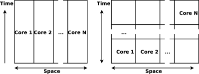
A key component of this enabling, next-generation simulation paradigm can likely be space-time parallel simulations. These simulations subdivide the 4-dimensional space-time computational domain. Each computing core handles a contiguous subdomain of the simulation space-time. Compared to subdivision only in the 3-dimensional space, space-time parallel simulations can achieve significantly higher level of concurrency, and reduce the ratio of inter-core communication to floating point operations. Each core computes the solution over a fraction of the entire simulation time window (Fig 3), reducing the simulation turnaround time.

Figure 3: Illustration of spatial parallelism (left) and space-time parallelism (right).

Space-time parallel simulations can significantly reduce the ratio of inter-core data transfer to floating point operations. This ratio can be estimated from the fraction of grid points lying on subdomain interfaces. The fraction of interfacial grid points in a spatially parallel simulation is estimated to be $\sim 6\left(M/N\right)^{-\frac{1}{3}}$, where $M$ is the total number of grid points assumed to be uniformly distributed in a cubical domain, and $N$ is the number of computing cores. The fraction of space-time grid points in a space-time parallel simulation is estimated to be $\sim 8\left(M\,T/N\right)^{-\frac{1}{4}}$, where $T$ is the total number of time steps. Table 1 shows that typical space-time parallel simulations on a million cores have significantly smaller ratio of inter-core data transfer to floating point operations than equivalent spatially parallel simulations.

$M$	$T$	$m_{so}$	$m_{st}$	$\tilde{m}_{so}$
$10^{6}$	$10^{5}$	$1$	$10^{5}$	$2.4\times 10^{3}$
$10^{7}$	$2\times 10^{5}$	$10$	$2\times 10^{6}$	$2.2\times 10^{4}$
$10^{8}$	$5\times 10^{5}$	$100$	$5\times 10^{7}$	$2.5\times 10^{5}$
$10^{9}$	$10^{6}$	$1000$	$10^{9}$	$2.4\times 10^{6}$

Table 1: For typical simulations of $M$ grid points and $T$ time steps running on $N=10^{6}$ cores, this table estimates the grid points per core of a spatially parallel simulation $m_{so}=M/N$, the space-time grid points per core of a space-time parallel simulation $m_{st}=M\,T/N$, and the equivalent grid points per core of a spatially parallel simulation with the same fraction of interfacial grid points as the space-time parallel simulation $6\tilde{m}_{so}^{-\frac{1}{3}}=8m_{st}^{-\frac{1}{4}}$. Space-time parallel simulations have significantly more effective grid points per core, which can lead to increased parallel efficiency.

If a space-time parallel simulation achieves the same parallel efficiency of a spatially parallel simulation for the same fraction of interfacial grid points, Table 1 and Fig 2 suggest that a typical million-grid-point turbulent flow simulation can run efficiently on a million cores with good parallel efficiency.

By reducing the ratio of inter-core communication to floating point operations, space-time parallel simulations has the potential of achieving high parallel efficiency, even for relatively small turbulent flow simulations on extreme scale parallel machines. Combined with next generation computing hardware, this could lead to typical simulation turnaround time of minutes. Space-time parallelism could enable high fidelity CFD-based design, including sensitivity analysis, optimization, control, uncertainty quantification and data-based inference.

II Barrier to efficient time parallelism

Time domain decomposition methods have a long history Nievergelt (1964). Popular methods include the multiple shooting method, time-parallel and space-time multigrid method, and the Parareal method.

Figure 4: Illustration of the Parareal algorithm, extracted from referenceReynolds-Barredo et al. (2012). $G$ and $F$ are the coarse and fine solvers, respectively.

As exemplified in Fig. 4, most time domain parallel methods divides the simulation time interval into small time chunks. They start with an initial estimate obtained by a coarse solver. Iterations are then performed over the entire solution history, aiming to converge to the solution of the initial value problem. In particular, the Parareal method has been demonstrated to converge for large scale turbulent plasma simulationsSamaddar, Newman, and Sánchez (2010); Reynolds-Barredo et al. (2012).

However, many time parallel methods suffer from a common scalability barrier in the presence of chaotic dynamics. The number of required iterations increases as the length of the time domain increases. As demonstrated for both the Lorenz attractorGander and Hairer (2008) and a turbulent plasma simulationReynolds-Barredo et al. (2012), the number of iterations for reaching a given tolerance is often proportional to the length of the time domain. Because the the number of operations per iteration is also proportional to the length of the time domain, the overall computation cost of most classical algorithms scales with the square of the time domain length. It is worth noting that recent developments have demonstrated a sub-quadratic cost scaling with time domain length via processor reuseBerry et al. (2012).

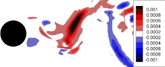
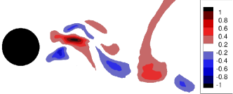
This poor scalability is related to the characteristic sensitivity of chaos. A small perturbation to a chaotic dynamical system, like the turbulent flow shown in Fig 5, can cause a large change in the state of the system at a later time.

(a) $t=2$

(b) $t=22$

(c) $t=62$

Figure 5: Spanwise velocity difference between two unsteady flow solutions at $t=2,22$ and $62$. A $10^{-5}$ magnitude perturbation at $t=0$ is the only difference between the two solutions. The growing magnitude of difference shows the ill-conditioning of a chaotic initial value problem. $Re_{D}=500$; periodic spanwise extent of $4D$ is used.

Figure 6: Error in 9 Parareal iterations of the Lorenz attractorGander and Hairer (2008) shows increasingly delayed convergence of later time chunks. Horizontal axis represent time chunks; each time chunk has length of 0.1.

Figure 7: Error in 12 Parareal iterations of a turbulent plasma simulation shows increasingly delayed convergence of later time chunks. Figure is extracted from referenceReynolds-Barredo et al. (2012). Horizontal axis represent time chunks. The solid red line represents the first iteration; the yellow dashed line at the lower right corner represents the 12th iteration.

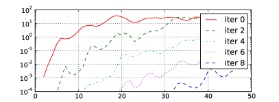
This sensitivity causes a significant barrier to fast convergence of time domain parallel methods. In the Parareal method, for example, a small difference between the coarse and fine solvers in the early time chunks can cause a large difference in the initial estimate and the converged solution. A small correction made in the earlier time chunks can result in a large update in later time chunks. As a result, the later time chunks can only converge after the earlier time chunks converge (Figs 6 and 7). The number of iterations required to converge the entire solution below a certain tolerance therefore increases as the length of the time domain increases.

The cause of this poor scalability, the sensitivity of chaos, can be quantified by the Lyapunov exponent. Consider two otherwise identical simulations with an infinitesimal difference in their initial condition. If the simulated system is chaotic, then the difference between these two simulations would grow as $\exp\lambda t$. This $\lambda$ is the maximal Lyapunov exponent, often just called as the Lyapunov exponent. Mathematically, for a dynamical system with an evolution function $\Phi^{t}(u)$,

$$\lambda=\lim_{t\rightarrow\infty}\lim_{\epsilon\rightarrow 0}\frac{1}{t}\log\frac{\|\Phi^{t}(u+\epsilon v)-\Phi^{t}(u)\|}{\|\epsilon v\|}$$

almost surely for any $v$ and $u$ on the attractor Strogatz (2001).

By describing how much a small perturbation changes the solution at a later time, the Lyapunov exponent $\lambda$ determines the convergence behavior of time domain parallel methods. A small error of magnitude $\epsilon$ at $t=0$ in a Parareal coarse solver can cause an error of size $\sim\epsilon\>e^{\lambda t}$ at a later time $t$. A small update of size $\epsilon$ at an earlier time $t_{1}$ can require an update of size $\sim\epsilon\>e^{\lambda(t_{2}-t_{1})}$ at a later time $t_{1}$. It is no surprise that a larger Lyapunov exponent $\lambda$ poses a greater challenge to time parallel methods like Parareal.

The influence of the Lyapunov exponent $\lambda$ on the convergence of Parareal is particularly significant in chaotic dynamical systems that have multiple time scales. The maximal Lyapunov exponent, with a unit of time^-1, is often inversely proportional to the smallest time scale. Consequently, time domain parallel methods are particularly challenged by chaotic multiscale simulations in which very small time scales are resolved.

Figure 8: A solution of the multiscale coupled Lorenz system (1) with $c=1/4$. The thick, red line indicates the slow variable $z_{s}$. The thin, blue line indicates the fast variable $z_{f}$.

Figure 9: Error in 9 Parareal iterations of the coupled Lorenz system (1) for $c=1/2$ (upper) and $c=1/4$ (lower). We observe slower convergence when a wider range of chaotic timescales are present. The horizontal axes represent time; each time chunk has length of 0.1. The coarse solver is forward Euler of step size $0.004\times c$; the fine solver is fifth order Runge Kutta with adaptive time stepping.

A simple example of such chaotic systems with multiple time scales is the coupled Lorenz system

$$\dot{x}_{s} =\sigma(y_{s}-x_{s}), c\,\dot{x}_{f} =\sigma(y_{f}-x_{f})$$ (1)

$$\dot{y}_{s} =x_{s}(r-z_{s})-y_{s}, c\,\dot{y}_{f} =x_{f}(r-z_{f})-y_{f}$$

$$\dot{z}_{s} =x_{s}y_{s}-\beta(z_{s}+z_{f}), c\,\dot{z}_{f} =x_{f}y_{f}-\beta(z_{s}+z_{f})$$

Fig. 8 shows that the coefficient $c<1$ determines the time scale of the fast dynamics, whereas the slower dynamics has a time scale of about 1. When $c$ decreases, the maximal Lyapunov exponent $\lambda$ increases. Figure 9 shows that Parareal converges proportionally slower for smaller $c$.

These pieces of evidence suggest that time domain parallel methods such as Parareal can suffer from lack of scalability in simulating chaotic multiscale systems, e.g., turbulent flows. The length of the time domain in a turbulent flow simulation is often multiples of the slowest time scale, so that converged statistics can be obtained. The finest resolved time scale that determines the maximal Lyapunov exponent can be orders of magnitude smaller than the time domain length. Consequently, the required number of time domain parallel iterations can be large. Increasing the time domain length or the resolved time scales would further increase the required number of iterations.

III Reformulating turbulent flow simulation

Time domain parallel methods, such as Parareal, scale poorly in simulation of chaotic, multiscale dynamical systems, e.g. turbulent flows. This poor scalability is because the initial value problem of a chaotic dynamical system is ill-conditioned. A perturbation of magnitude $\epsilon$ at the beginning of the simulation can cause a difference of $\epsilon\>\exp\lambda t$ at time $t$ later, where $\lambda$ is the maximal Lyapunov exponent. The condition number of the initial value problem can be estimated to be

$$\kappa\sim\exp\lambda T\sim\exp\frac{T}{\tau}\;,$$

where $T$ is the time domain length and $\tau$ is the smallest resolved chaotic time scale. This condition number can be astronomically large for multiscale simulations such as DNS and LES of turbulent flows. Efficient time domain parallelism can only be achieved through reformulating turbulent flow simulation into a well-conditioned problem.

We reformulate turbulent flow simulation into a well-conditioned problem by relaxing the initial condition. Not strictly enforcing an initial condition is justified under the following two assumptions:

1. Interest in statistics: all quantities of interest in the simulation are statistics of the flow field in quasi-equilibrium steady state. These include the mean, variance, correlation, high order moments and distributions of the flow field.

2. Ergodicity: starting from any initial condition, the flow will reach the same quasi-equilibrium steady state after initial transient. All statistics of the flow field are independent of the initial condition after reaching the quasi-equilibrium steady state.

Under these assumptions, satisfying a particular initial condition is not important to computing the quantities of interest. Instead of trying to find the flow solution that satisfies both the governing equation and the initial condition, we aim to find a flow solution satisfying only the governing equation. For example, we can formulate the problem as finding the solution of the governing equation that is closest (in $L^{2}$ sense) to a reference solution, which can come from a coarse solver or from solution at a different parameter value.

Note that we do not address dynamic measures such as time domain correlations and power spectra. Further analysis is required to assess whether these dynamic measures are captured by the present method.

Relaxing the initial condition annihilates the ill-conditioning in simulating chaotic dynamical systems, making time parallelization efficient and scalable. If the initial condition were fixed, a small perturbation near the beginning of the simulation would cause a large change in the solution later on. If the initial condition were relaxed, a small perturbation near the beginning of the simulation could be accommodated by a small change in the initial condition, with little effect on the the solution after the perturbation.

Figure 10: A geometric illustration of the response of a chaotic dynamical system to an impulse perturbation. The black arrow represents an unperturbed trajectory running along the $z$-axis. The red arrows represent the perturbation. The magenta dashed line represents the perturbed trajectory with fixed initial condition. The blue line represents a perturbed trajectory with relaxed initial condition.

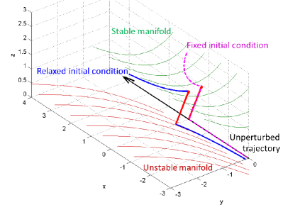
The following geometric analysis demonstrates the stability of a chaotic dynamical system with relaxed initial condition. The phase space around a trajectory can be decomposed into a stable manifold and an unstable manifold. Consider an arbitrary impulse perturbation to the system as shown in Fig 10. Because the perturbation can contain a component along the unstable manifold, the perturbed trajectory would exponentially diverge from the unperturbed trajectory if the initial condition were fixed. However, If the initial condition is relaxed, the perturbation along the unstable manifold can be annihilated by slightly adjusting the initial condition, as shown in Fig 10. This small adjustment in the initial condition makes it sufficient to only consider the decaying effect of the perturbation along the stable manifold. The effect of the perturbation along the unstable manifold is reflected by the small trajectory change before the perturbation.

Stability of the trajectory with a relaxed initial condition is achieved by splitting a perturbation into stable and unstable components, and propagating their effects forward and backward in time, respectively. This stability property is formally known as the Shadowing Lemma Pilyugin (1999). Consider a dynamical system governed by

$$\frac{du}{dt}=\mathcal{R}(u)\;,$$

where $\mathcal{R}$ is a nonlinear spatial operator. The shadowing lemma states that For any $\delta>0$ there exists $\epsilon>0$, such that for every $u_{r}$ that satisfies $\|\partial u_{r}/\partial\tau-\mathcal{R}(u_{r})\|<\epsilon\,,\;0\leq t\leq T\,,$ there exists a true solution $u$ and a time transformation $t(\tau)$, such that $\|u(\tau)-u_{r}(\tau)\|<\delta$, $|1-dt/d\tau|<\delta$, and $\partial u/\partial t-\mathcal{R}(u)=0\,,\;0\leq\tau\leq T$.

(a) Solutions of initial value problems

(b) Solutions of the reformulated system

Figure 11: Comparison between solutions of initial value problems of the Lorenz system (left, showing extreme sensitivity to $\rho$) and the reformulated system (2) (right, showing smooth dependence on $\rho$). Note that the solutions of the reformulated system at different values of $\rho$ “shadow” each other. The difference in the physical time $t$ and the shadowing time $\tau$ is the effect of nonzero time dilation $\eta(\tau)$.

The shadowing lemma theorizes the trajectory stability of chaotic dynamical systems with relaxed initial conditions. This paper develops the following least squares formulation designed to take advantage of this stability numerically

$$\begin{split}u,\eta&=\operatornamewithlimits{argmin}\frac{1}{2}\int_{0}^{T}\Big{(}\|u(\tau)-u_{r}(\tau)\|^{2}+\eta(\tau)^{2}\Big{)}d\tau\\ &\mbox{s.t.}\quad(1+\eta)\frac{\partial u}{\partial\tau}=\mathcal{R}(u)\;,\quad 0\leq\tau\leq T\end{split}$$ (2)

This least squares problem finds a solution $u(\tau)$ satisfying the differential equation

$$\frac{\partial u(\tau(t))}{\partial t}=\mathcal{R}(u)$$

with a time transformation $\tau$ satisfying $d\tau/dt=1+\eta(\tau)$. Here the scalar function of time $\eta(\tau)$ is part of the solution to the least squares problem. The solution $u(\tau),\eta(\tau)$ minimizes a combination of two metrics, (a) the distance between $u(\tau)$ and a reference solution $u_{r}(\tau)$, and (b) the deviation from unity of the time transformation, represented by $\eta(\tau)$.

The least squares problem (2) has a unique and stable solution when the reference solution $u_{r}$ is close to the actual solution $u$, so that $u-u_{r}$ can be described by the corresponding linearized least squares problem. With a convex, positive definite objective function and a linear constraint, this problem has a unique and stable solution.

The constraint least squares problem (2) can be simplified by forming its Lagrange function

$$\begin{split}\Lambda=\int_{0}^{T}&\bigg{(}\frac{\langle u-u_{r},u-u_{r}\rangle+\eta^{2}}{2}+\Big{\langle}w,\frac{\partial u}{\partial t}-\mathcal{R}(u)\Big{\rangle}\bigg{)}\,dt\end{split}$$ (3)

where $w$ is the Lagrange multiplier. Variation of the Lagrange function can be transformed through integration by parts

$$\begin{split}\delta\Lambda=&\int_{0}^{T}\delta\eta\Big{(}\eta+\Big{\langle}w,\frac{\partial u}{\partial\tau}\Big{\rangle}\Big{)}+\langle\delta u,u-u_{r}\rangle+\Big{\langle}w,\frac{\partial\delta u}{\partial t}-\mathcal{L}\delta u\Big{\rangle}\,dt\\ =&\int_{0}^{T}\Big{\langle}\delta u\;,\;u-u_{r}-\frac{\partial w}{\partial t}-\mathcal{L}^{*}w\Big{\rangle}\,dt+\int_{0}^{T}\delta\eta\;\Big{(}\eta+\Big{\langle}w\;,\;\frac{\partial u}{\partial\tau}\Big{\rangle}\Big{)}\,dt+\langle\delta u,w\rangle\bigg{|}_{0}^{T}\end{split}$$ (4)

where $\mathcal{L}$ is the linearized operator

$$\mathcal{L}=\left.\frac{\delta\mathcal{R}(u)}{\delta u}\right|_{u_{r}}\;,$$ (5)

$\mathcal{L}^{*}$ is the adjoint operator of $\mathcal{L}$. The solution of the constraint least squares problem (2) satisfies the first order optimality condition $\delta\Lambda=0$ for all $\delta u$ and $\delta\eta$. Therefore, Equation (4) leads to

$$u=u_{r}+\frac{\partial w}{\partial t}+\mathcal{L}^{*}w\;,\quad\eta=-\Big{\langle}w\;,\;\frac{\partial u}{\partial\tau}\Big{\rangle}$$ (6)

and the boundary condition $w(\tau=0)=w(\tau=T)=0$.

Substituting these equalities back into the constraint in (2), we obtain the following second order boundary value problem in time:

$$\begin{split}&\frac{\partial}{\partial t}\left(\frac{\partial w}{\partial t}+\mathcal{L}^{*}w+u_{r}\right)-\mathcal{R}\left(\frac{\partial w}{\partial t}+\mathcal{L}^{*}w+u_{r}\right)=0\\ &w\big{|}_{\tau=0}=w\big{|}_{\tau=T}=0\;,\end{split}$$ (7)

where the transformed time derivative is

$$\frac{\partial}{\partial t}=(1+\eta)\,\frac{\partial}{\partial\tau}\;.$$ (8)

Our reformulation of chaotic simulation produces a least squares system (2), whose solution $u$ satisfies the governing equation, and has relaxed initial condition. This solution can be found by first solving the Lagrange multiplier $w$ through Equation (7), a second order boundary value problem in time, then computing $u$ from Equation (6). As illustrated in Figure 11, this reformulated problem does not suffer from ill-conditioning found in initial value problems of chaos, therefore overcomes a fundamental barrier to efficient time-parallelism. The reformulated boundary value problem in time (7) is well-conditioned and suitable for time domain parallel solution methods. These properties are demonstrated mathematically in Section IV and Appendix A, and through examples in Sections V and VI.

IV Solving the reformulated system

Solving the reformulated problem involves two steps: 1. solving a nonlinear boundary-value-problem in time (7) for the Lagrange multiplier $w$, and 2. evaluating Equation (6) for the solution $u$. Performing the second step in space-time parallel is relatively straightforward. This section introduces our iterative algorithm for the first step based on Newton’s method.

1. Decompose the 4D spatial-temporal computational domain into subdomains.

2. Start at iteration number $k=1$ with an initial guess $u^{(0)}$ distributed among computing cores.

3. Compute the residual $du^{(k-1)}/dt-\mathcal{R}(u^{(k-1)})$ in each subdomain. Terminate if the magnitude of the residual meets the convergence criteria.

4. Solve a linearized version of Equation (7) for $w^{(k)}$ using a space-time parallel iterative solver (detailed follows in the rest of this section).

5. Compute the time dilation factor $\eta$ and transformed time $dt=d\tau\,\exp\,(-\eta(\tau))$.

6. Compute the updated solution $u^{(k)}$ by parallel evaluation of Equation (6) with $u_{r}=u^{(k-1)}$ and $w=w^{(k)}$.

7. Update to transformed time by letting $\tau=t$; continue to Step 3 with $k=k+1$.

Note that the update in Step 5 avoids degeneracy when $\eta\leq-1$, and is first order consistent with $dt=d\tau/(1+\eta(\tau))$ implied by the definition of $\eta$. Numerically, this step is involves updating each physical time step size $\Delta t_{i}$ from the corresponding shadowing time step size $\Delta\tau_{i}$, while keeping the number of time steps fixed.

The only step that requires detailed further explanation is Step 4. All other steps can be evaluated in space-time parallel with minimal communication across domain boundaries. Solving Equation (7) for $w$ using Newton’s method requires a linear approximation to the equation. Ignoring second order terms by assuming both $u-u_{r}$ and $\eta$ are small, Equation (7) becomes

$$\begin{split}-&\frac{\partial^{2}w}{\partial\tau^{2}}-\left(\frac{\partial}{\partial\tau}\mathcal{L}^{*}-\mathcal{L}\frac{\partial}{\partial\tau}\right)w+\big{(}\mathcal{L}\mathcal{L}^{*}+\mathcal{P}\big{)}w=f_{\tau}\\ &w\big{|}_{\tau=0}=w\big{|}_{\tau=T}=0\;,\end{split}$$ (9)

where $\mathcal{P}$ is a symmetric positive semi-definite spatial operator

$$\mathcal{P}w=\left\langle w\,,\;\frac{\partial u_{r}}{\partial t}\right\rangle\frac{\partial u_{r}}{\partial t}\;.$$ (10)

and

$$f_{\tau}=\frac{\partial u_{r}}{\partial\tau}-\mathcal{R}(u_{r})$$ (11)

It can be shown that the system (9) is a symmetric positive definite system with good condition number (see Appendix A). It also has a energy minimization form, allowing a standard finite element discretization. Appendix B details the discretization and the numerics of solving Equation (9).

We implemented both a direct solver and an iterative solver for the symmetric boundary value problem (9). The computation time of both methods is analyzed in Appendix B. The total cost of a direct parallel solution method (cyclic reduction) is estimated to be 10 times that of solving a linear initial value problem of the same size using implicit time stepping and Gauss elimination in each time step. If a parallel iterative solution method (multigrid-in-time Brandt (1981)) is used, the total computation cost of solving Equation (9) with $n_{iter}$ total smoothing iterations is about 6 times that of solving a linear initial value problem of the same size, with $n_{iter}$ iterations performed in solving each implicit time step. Our naive implementation of multigrid-in-time requires an $n_{iter}$ ranging from 100 to 1000 for the Lorenz system and the Kuramoto-Sivashinsky equation. This number could be reduced through more research into iterative solution algorithm specifically for Equation (9). When the operator $\mathcal{L}$ is a large scale spatial operator, we envision that the multigrid-in-time method can be extended to a space-time multigrid method.

V Validation on the Lorenz System

The algorithm described in Section IV is applied to the Lorenz system. Both the solution $u(t)$ and the Lagrange multiplier $w(t)$ in this case are in the Euclidean space $R^{3}$. The three components of the solution are denoted as $u(t)=(x,y,z)$ by convention. The governing equation is

$$\dot{u}=\mathcal{R}(u)=\Big{(}s(y-x),\;x(r-z)-y,\;xy-bz\Big{)}\;,$$ (12)

where $s=10$, $r=35$ (the Rayleigh number) and $b=8/3$ are three parameters of the system.

Figure 12: Solution of the Lorenz system at $s,r,b=10,{\bf 35},8/3$ with the algorithm of Section IV. The initial guess $u^{(0)}(t),t\in[0,100]$ is a solution of the system at $s,r,b=10,{\bf 25},8/3$. The horizontal axis indicates the iteration number $k$. The dot-dash line with open triangles indicates the norm of the residual $f_{\tau}^{(k)}$. The red, solid line with filled circles represents the time averaged $z$ of the solution $u^{(k)}$. The horizontal dashed line indicates the mean $z$ computed from an independent initial value solution at $r={\bf 35}$.

The initial guess $u^{(0)}$ used in Section IV’s algorithm is a numerical solution of the system at a different Rayleigh number $r=25$. The initial guess has 10,001 time steps uniformly distributed in a time domain of length 100. Appendix B discusses the details of the numerics.

Figure 13: The black trajectory is a phase space plot of the initial guess $u^{(0)}$, a solution of the Lorenz system at $s,r,b=10,{\bf 25},8/3$. The red trajectory plots the converged solution $u^{(10)}$, a least squares solution of the Lorenz system at $s,r,b=10,{\bf 35},8/3$.

Figure 14: The blue, dashed line represents $z(\tau)$ of the initial guess, a solution of the system at $r=25$. The red, solid line represents $z(t)$ of the converged solution at $r=35$.

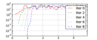
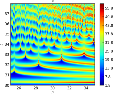
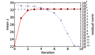
As a general rule in Newton’s method for solving nonlinear systems, the algorithm described in Section IV is expected to converge only when the initial guess is sufficiently close to the solution. In fact, we rarely observe convergence to a physical solution if one starts from an arbitrary constant initial guess. However, we do observe convergence when the initial guess is obtained from a solver with a much large time step size, or when the initial guess is a qualitatively similar solution at a different parameter value. The example shown in Figures 12, 13 and 14 has a challenging initial guess at a very different parameter value ($\rho=25$ versus $35$.) The final solution has an averaged magnitude of over $50\%$ large than the initial guess.

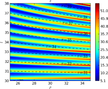
Figure 12 shows that the Newton’s iterations described in Section IV converges to machine precision within 9 iterations. Less iterations are required when the initial guess is closer to the final solution. The phase space plots in Figure 13 shows that the converged trajectory lies on the attractor of the Lorenz system at $r=35$, and is significantly different from the initial guess trajectory. Figure 14 shows that the converged trajectory closely tracks the initial guess trajectory on a transformed time scale. The statistical quantity (mean $z$) of the converged solution matches that computed from a conventional time integration.

Figure 15: Speed up of the multigrid-in-time solver of the linearized system (9) using up to 128 cores. 4096 time steps are allocated per core with uniform time step size of 0.01. The same convergence criterion is used for all cases.

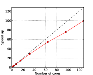
Because the reformulated system do not suffer from the ill-conditioning of the initial value problem, parallelization in time domain does not encounter the same problem as Parareal method for solving initial value problems. Figure 15 shows that our algorithm is scalable up to a time domains of length over 5000. In comparison, Parareal would take many more iterations to converge on longer time domains. Converging on a time domain of length 5000 would require over 500 Parareal iterations based on estimates from Figure 6.

VI Validation on the KS Equation

The algorithm described in Section IV is applied to the Kuramoto-Sivashinsky equation. Both the solution $u(x,t)$ and the Lagrange multiplier $w(x,t)$ in this case are functions in the spatial domain of $x\in[0,100]$. They also both satisfy the boundary conditions

$$u\Big{|}_{x=0,100}=\frac{\partial u}{\partial x}\bigg{|}_{x=0,100}=0$$

The governing equation is defined by

$$\frac{\partial u}{\partial t}=\mathcal{R}(u)=-(u+c)\frac{\partial u}{\partial x}-\frac{\partial^{2}u}{\partial x^{2}}-\frac{\partial^{4}u}{\partial x^{4}}\;,$$ (13)

Figure 16: Initial value solution of the Kuramoto-Sivashinsky equation (13) for $c=-1$ (left) and $c=-0.1$ (right). Finite difference discretization on 128 uniform spatial gridpoints is used. The initial condition in both cases use i.i.d. uniform $[-\frac{1}{2},\frac{1}{2}]$ random numbers.

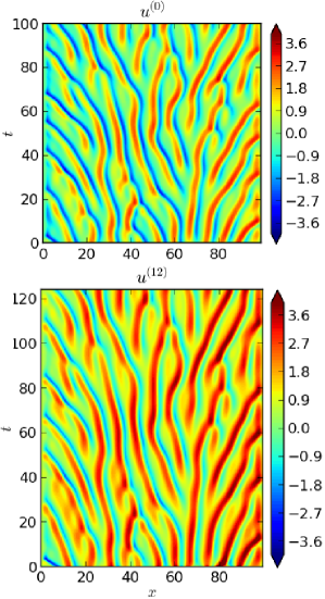
where the parameter $c$ is introduced to control the behavior of the system. Figure 16 shows that solutions of this initial boundary value problem at $c=-0.1$ and $c=-1$ reach different chaotic quasi-equilibrium after starting from similar initial conditions. The mean of the solution at equilibrium is higher in the $c=-1$ case than in the $c=-0.1$ case.

Figure 17: Solution of the Kuramoto-Sivashinsky (KS) equation (13) at $c=-1$ with the algorithm of Section IV. The initial guess $u^{(0)}(x,t),x\in[0,100],t\in[0,50]$ is a solution of the KS equation at $c=-0.1$. The horizontal axis indicates the iteration number $k$. The dot-dash line with open triangles indicates the norm of the residual $f_{\tau}^{(k)}$. The red, solid line with filled circles represents the solution $u^{(k)}(x,t)$ averaged over $x$ and $t$. The horizontal dashed line indicates the averaged $u(x,t)$ computed from an independent initial value problem at $c=-1$.

Section IV’s algorithm is tested for the Kuramoto-Sivashinsky equation at $c=-1$. The initial guess $u^{(0)}$ is a numerical solution of the Kuramoto-Sivashinsky equation at $c=-0.1$. This initial guess has 401 time steps uniformly distributed in a time domain of length 100. Appendix B discusses the details of the numerics.

Figure 18: The initial guess $u^{(0)}$ and the converged solution $u^{(12)}$ in Section IV’s algorithm applied to the Kuramoto-Sivashinsky equation (13) at $c=-1$.

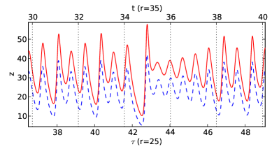
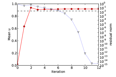
The Newton’s iteration converges even though the initial guess has an advection velocity $c$ that is 10 times lower than the solution. Figure 17 shows that the algorithm of Section IV converges on the Kuramoto-Sivashinsky equation to machine precision within about 10 iterations. The statistical quantity (mean $u$) of the converged solution is close to that computed from a time integration. The small discrepancy between them may be caused by the difference between the infinite time statistical average and the finite time average over the time domain length of about 120. Figure 18 shows that the converged solution shadows the initial condition on a stretched time scale.

VII Conclusion

We used the ergodic hypothesis to relax the initial condition in simulating chaotic, unsteady dynamical systems. The system with relaxed initial condition do not suffer from ill-conditioning encountered in fixed-initial condition problems. Consequently, efficient parallel-in-time simulation can be performed without scalability problems from which time parallelization of initial value problem suffers. The relaxed-initial-condition system is formulated into a least squares problem, whose solution can be obtained through a second order boundary value problem in time. We solve this boundary value problem using an iterative solution algorithm based on Newton’s method. All steps in the algorithm can be efficiently performed in time-parallel.

This methodology is demonstrated on simulations of the Lorenz system and the Kuramoto-Sivashinsky equation. The iterative algorithm converges in both cases to machine precision solutions within 10 iterations. The statistical quantities of the converged solutions with relaxed initial conditions match those computed from traditional time integration methods. Time parallel scalability of this method is demonstrated on the Lorenz attractor.

In summary, the primary advantages of this methodology are

1. Scalable time-parallelism. The reformulation can enable a new class of time-parallel and space-time-parallel computational simulation codes that effectively use next generation exascale computers.

2. Well-conditioning. The proposed formulation can be proved to have low condition numbers, making many simulated-based computational methods, e.g., optimization, uncertainty quantification and inference easier to apply.

The associated disadvantages of this methodology are mainly

1. Increased number of floating point operations. The total number of floating point operations is estimated to be 6 to 10 times that of solving an initial value problem of the same size using implicit time stepping. The ratio can potentially be higer if a larger number of Newton iterations or linear solver iterations are required.

2. Requiring a initial guess. We observe that the initial guess must be qualitatively similar to a physical solution in order for the Newton’s method to converge.

3. Requiring research and developement of new solvers. Research is need to investigate iterative linear solvers that are efficient for the large scale linear system involved in this methodology. Existing solvers based on initial value problems have to be rewritten to solve the reformulated system.

VIII Acknowledgments

The authors thank financial support from NASA Award NNX12AJ75A through Dr. Harold Atkins, AFOSR STTR contract FA9550-12-C-0065 through Dr. Fariba Farhoo, and a subcontract of DOE’s Stanford PSAAP to MIT. The coauthors were supported by the ANSYS fellowship at MIT Aerospace Computing and Design Lab and the NASA graduate summer internship at Langley during the work.

Appendix A Well conditioned

The linearized equation (9) also has a weak form

$${\mathfrak{a}}(\delta w,w)+{\mathfrak{l}}(\delta w)=0$$ (14)

and an energy minimization form, which is the Lagrangian dual of the linearized least squares (2),

$$w=\operatornamewithlimits{argmin}_{w|_{0,T}=0}\left(\frac{{\mathfrak{a}}(w,w)}{2}+{\mathfrak{l}}(w)\right)\;,$$ (15)

The symmetric, positive definite and well-conditioned bilinear form $\mathfrak{a}$ is

$${\mathfrak{a}}(w,v)=\int_{0}^{T}\left\langle\frac{\partial w}{\partial\tau}+\mathcal{L}^{*}w,\frac{\partial v}{\partial\tau}+\mathcal{L}^{*}v\right\rangle+\left\langle w,\mathcal{P}v\right\rangle\,d\tau$$ (16)

and linear functional $\mathfrak{l}$ is

$${\mathfrak{l}}(w)=\int_{0}^{T}\big{\langle}w,f_{\tau}\big{\rangle}\,d\tau\;.$$ (17)

The derivation and properties of the weak and energy forms are detailed in Appendix A. These forms of Equation (9) makes it possible to achieve provable convergence of iterative solution techniques.

By taking the inner product of a test function $v$ with both sides of Equation (9), integrating over the time domain $[0,T]$, and using integration by parts, we obtain

$$\int_{0}^{T}\left\langle\frac{\partial w}{\partial\tau}+\mathcal{L}^{*}w,\frac{\partial v}{\partial\tau}+\mathcal{L}^{*}v\right\rangle+\left\langle w,\mathcal{P}v\right\rangle-\big{\langle}v,f_{\tau}\big{\rangle}\,d\tau=0\;,$$ (18)

which is the weak from (14). We decompose the solution $w$ into the adjoint Lyapunov eigenvectors in order to show that the symmetric bilinear form $\mathfrak{a}(u,v)$ as in Equation (16) is positive definite and well-conditioned. The Lyapunov decomposition for an $n$-dimensional dynamical systems (including discretized PDEs) is

$$w(t)=\sum_{i=1}^{n}w_{i}(t)\phi_{i}(t)\;,\quad\mbox{where}\quad\frac{\partial\phi_{i}}{\partial t}+\mathcal{L}^{*}\phi_{i}=\lambda_{i}\phi_{i}$$ (19)

Each $w_{i}$ is a real valued function of $t$, and $\phi_{i}(t)$ is the corresponding adjoint Lyapunov eigenvectors. By convention, the Lyapunov exponents are sorted such that $\lambda_{i}\geq\lambda_{i+1}$. Combining the Lyapunov eigenvector decomposition (19) results in

$$\frac{\partial w}{\partial\tau}+\mathcal{L}^{*}w=\sum_{i=1}^{n}\left(\frac{dw_{i}}{d\tau}+\lambda_{i}w_{i}\right)\phi_{i}$$

By substituting this equality and Equations (10) into the bilinear form and using the positive semi-definiteness of $\mathcal{P}$, we obtain

$$\begin{split}&\mathfrak{a}(w,w)\geq\\ &\int_{0}^{T}\sum_{i,j=1}^{n}\Big{(}\frac{dw_{i}}{d\tau}+\lambda_{i}w_{i}\Big{)}\Big{(}\frac{dw_{j}}{d\tau}+\lambda_{j}w_{j}\Big{)}\langle\phi_{i},\phi_{j}\rangle\,d\tau\end{split}$$ (20)

The eigenvalues of the matrix $\Big{(}\langle\phi_{i},\phi_{j}\rangle\Big{)}_{i,j=1,\ldots,n}$ are bounded away from both zero and infinity for uniformly hyperbolic dynamical systems, i.e., there exists $0<c\leq C<\infty$ such that

$$\begin{split}c\sum_{i=1}^{n}x_{i}^{2}<\sum_{i,j=1}^{n}x_{i}\,x_{j}\langle\phi_{i},\phi_{j}\rangle<C\sum_{i=1}^{n}x_{i}^{2}\end{split}$$ (21)

for any $x_{1},\ldots,x_{n}$. By applying these bounds to $\langle w,w\rangle$ and to Equation (20), we obtain

$$\begin{split}\mathfrak{a}(w,w)&>c\sum_{i=1}^{n}\int_{0}^{T}\left(\frac{dw_{i}}{d\tau}+\lambda_{i}w_{i}\right)^{2}\,d\tau\\ \langle w,w\rangle&<C\sum_{i=1}^{n}\int_{0}^{T}w_{i}^{2}\,d\tau\end{split}$$ (22)

Most high dimensional, ergodic chaotic systems of practical interest are often assumed to be quasi-hyperbolic, whose global properties are not affected by their non-hyperbolic nature. Therefore we conjecture that (22) also holds for these quasi-hyperbolic systems when $T$ is sufficiently large. Because of the boundary conditions $w(0)=w(T)=0$,

$$\begin{split}&\int_{0}^{T}\left(\frac{dw_{i}}{d\tau}+\lambda_{i}w_{i}\right)^{2}\,d\tau\\ =&\int_{0}^{T}\left(\frac{dw_{i}}{d\tau}\right)^{2}d\tau+\lambda_{i}\underbrace{\int_{0}^{T}w_{i}\frac{dw_{i}}{d\tau}\,d\tau}_{=0}+\lambda_{i}^{2}\underbrace{\int_{0}^{T}w_{i}^{2}\,d\tau}_{\geq 0}\\ \geq&\int_{0}^{T}\left(\frac{dw_{i}}{d\tau}\right)^{2}d\tau\end{split}$$ (23)

Also because of the boundary conditions, each $w_{i}(t)$ admits a Fourier sine series

$$w_{i}(t)=\sum_{m=1}^{\infty}\hat{w}_{im}\sin\frac{m\pi t}{T}\,,=\sum_{m=1}^{\infty}\hat{w}_{im}\,\frac{m\pi}{T}\cos\frac{m\pi t}{T}\;.$$ (24)

thus,

$$\frac{dw_{i}}{d\tau}=\sum_{m=1}^{\infty}\hat{w}_{im}\,\frac{m\pi}{T}\cos\frac{m\pi t}{T}\;.$$ (25)

The Parseval identity applies to both orthogonal series, leading to the Poincare inequality

$$\begin{split}&\int_{0}^{T}\left(\frac{dw_{i}}{d\tau}\right)^{2}d\tau=\frac{T}{2}\sum_{m=1}^{\infty}\hat{w}_{im}^{2}\underbrace{\left(\frac{m\pi}{T}\right)^{2}}_{\geq\left(\pi/T\right)^{2}}\\ \geq&\left(\frac{\pi}{T}\right)^{2}\frac{T}{2}\sum_{m=1}^{\infty}\hat{w}_{im}^{2}=\left(\frac{\pi}{T}\right)^{2}\int_{0}^{T}w_{i}^{2}\,d\tau\end{split}$$ (26)

By combining this inequality with the inequalities (22) and (23), we obtain

$$\frac{\mathfrak{a}(w,w)}{\langle w,w\rangle}>\left(\frac{\pi}{T}\right)^{2}\frac{c}{C}$$ (27)

This inequality leads to our conclusion that the symmetric bilinear form $\mathfrak{a}(w,v)$ is positive definite. Equation (9) is well-conditioned because if the weak form (14) holds and $\mathfrak{a}(w,w)=\mathfrak{l}(w)$, then

$$\|\mathfrak{l}\|\|w\|\geq\mathfrak{l}(w)=\mathfrak{a}(w,w)>\left(\frac{\pi}{T}\right)^{2}\frac{c}{C}\|w\|^{2}\;,$$ (28)

therefore,

$$\frac{\|w\|}{\|\mathfrak{l}\|}<\left(\frac{\pi}{T}\right)^{2}\frac{C}{c}\;.$$ (29)

This inequality bounds the magnitude of the solution by the magnitude of the perturbation. It also bounds the magnitude of the solution error by the magnitude of the residual. This condition number bound is $C/c$ times that of the Poisson equation in a 1D domain $[0,T]$.

Appendix B Discretization and numerical solution

Equation (15) can be solved using the Ritz method, which is equivalent to applying Galerkin projection on (9). The time domain $[0,T]$ is discretized into $n$ intervals by $0=\tau_{0}<\tau_{1}<\ldots<\tau_{n}=T$. Both the trial function $w$ and the test function $v$ are continuous function that is piecewise linear (i.e., linear within each interval $\tau_{i-1}\leq\tau\leq\tau_{i}$). The operators $\mathcal{L}^{*}$ and $\mathcal{P}$ are approximated as piecewise constant. Denote $w_{i}=w(\tau=\tau_{i}),i=0,\ldots,n$, $\mathcal{L}^{*}_{i}=\mathcal{L}^{*}(\tau_{i-1}<\tau<\tau_{i})$ and $\mathcal{P}_{i}=\mathcal{P}(\tau_{i-1}<\tau<\tau_{i})$, Equation (16) can be written as

$${\mathfrak{a}}(w,v)=\Big{(}v_{1}^{T}\,v_{2}^{T}\,\ldots\,v_{n-1}^{T}\Big{)}\left(\begin{array}[]{cccc}A_{1}&B_{2}&&\\ B_{2}^{T}&A_{2}&\ddots&\\ &\ddots&\ddots&B_{n-1}\\ &&B_{n-1}&A_{n-1}\end{array}\right)\left(\begin{array}[]{c}w_{1}\\ w_{2}\\ \vdots\\ w_{n-1}\end{array}\right)$$

where

$$A_{i}=\frac{I}{\Delta t_{i+1}}+\frac{I}{\Delta t_{i}}+\mathcal{L}_{i}+\mathcal{L}^{*}_{i}-\mathcal{L}_{i+1}-\mathcal{L}^{*}_{i+1}+\frac{\Delta t_{i}}{3}\Big{(}\mathcal{L}_{i}\mathcal{L}^{*}_{i}+\mathcal{P}_{i}\Big{)}+\frac{\Delta t_{i+1}}{3}\Big{(}\mathcal{L}_{i+1}\mathcal{L}^{*}_{i+1}+\mathcal{P}_{i+1}\Big{)}$$

$$B_{i}=-\frac{I}{\Delta t_{i}}+\mathcal{L}^{*}_{i}+\mathcal{L}_{i}+\frac{\Delta t_{i}}{6}\Big{(}\mathcal{L}_{i}\mathcal{L}^{*}_{i}+\mathcal{P}_{i}\Big{)}$$

Therefore, Equation (9) can be solved through a symmetric, positive definite, block-tridiagonal system

$$\left(\begin{array}[]{cccc}A_{1}&B_{2}&&\\ B_{2}^{T}&A_{2}&\ddots&\\ &\ddots&\ddots&B_{n-1}\\ &&B_{n-1}&A_{n-1}\end{array}\right)\left(\begin{array}[]{c}w_{1}\\ w_{2}\\ \vdots\\ w_{n-1}\end{array}\right)=\left(\begin{array}[]{c}l_{1}\\ l_{2}\\ \vdots\\ l_{n-1}\end{array}\right)$$ (30)

This system (30) can be solved in parallel using either direct or iterative method. The estimated computational runtime of a drect and an iterative parallel method are listed below. Here $N$ is the number of domain decompositions in the time domain. $M$ is the spatial degree of freedom, i.e., the size of the blocks $A_{i}$ and $B_{i}$ in (30).

1. Parallel cyclic reduction is efficient when the $M$ is small and the spatial operator $\mathcal{L}$ is dense. Its estimated computation time is Seal, Perumalla, and Hirshman (2013)

   $$(C_{in}+6\,C_{mm})M^{3}\left(\frac{n}{N}+\log N\right)+2\beta M^{2}\left(\log\frac{n}{N}+2\log n\right)\;,$$

   where $C_{in}$, $C_{mm}$ are the amortized time per floating point operation for matrix inversion and matrix-matrix multiplication, respectively. $\beta$ is the average time to transmit one floating point number between any two processing elements across the network.

   In particular, when a single processor is used, i.e., $N=1$, the computation time is about a factor of 10 higher than solving a $M$-dimensional linear initial value problem with $N$ time steps using implicit time stepping, where the linear system in each time step is solved using Gauss elimination.

2. V-cycle parallel multigrid is efficient when $M$ is large and the spatial operator $\mathcal{L}$ is sparse. Assume that the matrix representation of $\mathcal{L}$ has on average $n_{nz}$ nonzero entries per row. A multigrid cycle containing $n_{s}$ pre- and post-smoothing Jacobi-like iterations has an estimated computation time of

   $$6\,C_{mv}Mn_{nz}n_{s}\frac{n}{N}+2\beta Mn_{s}\log\frac{n}{N}\;,$$

   where $C_{mv}$ is the amortized time per floating point operation for sparse matrix-vector multiplication. $\beta$ is the average time to transmit one floating point number between any two processing elements across the network.

   In particular, when a single processor is used, i.e., $N=1$, the computation time of $n_{cyc}$ multigrid cycles is similar to that of solving a $M$-dimensional linear initial value problem with $N$ time steps using implicit time stepping, where the linear system in each time step is solved using iterative method involving $6\,n_{cyc}\,n_{mv}$ Jacobi-like iterations.

References

- Sagaut (2001) P. Sagaut, “Large eddy simulation for incompressible flows. an introduction,” Measurement Science and Technology 12, 1745 (2001).
- Pitsch (2006) H. Pitsch, “Large-eddy simulation of turbulent combustion,” Annual Review of Fluid Mechanics 38, 453–482 (2006).
- Marsden et al. (2007) A. L. Marsden, M. Wang, Dennis, Jr, and P. Moin, “Trailing-edge noise reduction using derivative-free optimization and large-eddy simulation,” Journal of Fluid Mechanics 572, 13–36 (2007).
- Ruelle (1997) D. Ruelle, “Differentiation of SRB states,” Communications in Mathematical Physics 187, 227–241 (1997).
- Kogge et al. (2008) P. Kogge, K. Bergman, S. Borkar, D. Campbell, W. Carson, W. Dally, M. Denneau, P. Franzon, W. Harrod, K. Hill, et al., “Exascale computing study: Technology challenges in achieving exascale systems,” (2008).
- Amarasinghe et al. (2009) S. Amarasinghe, D. Campbell, W. Carlson, A. Chien, W. Dally, E. Elnohazy, M. Hall, R. Harrison, W. Harrod, K. Hill, et al., “Exascale software study: Software challenges in extreme scale systems,” DARPA IPTO, Air Force Research Labs, Tech. Rep (2009).
- Moin (2002) P. Moin, “Advances in large eddy simulation methodology for complex flows,” International journal of heat and fluid flow 23, 710–720 (2002).
- Nievergelt (1964) J. Nievergelt, “Parallel methods for integrating ordinary differential equations,” Communications of the ACM 7, 731–733 (1964).
- Reynolds-Barredo et al. (2012) J. Reynolds-Barredo, D. Newman, R. Sanchez, D. Samaddar, L. Berry, and W. Elwasif, “Mechanisms for the convergence of time-parallelized, parareal turbulent plasma simulations,” Journal of Computational Physics (2012).
- Samaddar, Newman, and Sánchez (2010) D. Samaddar, D. E. Newman, and R. Sánchez, “Parallelization in time of numerical simulations of fully-developed plasma turbulence using the parareal algorithm,” J. Comput. Phys. 229, 6558–6573 (2010).
- Gander and Hairer (2008) M. Gander and E. Hairer, “Nonlinear convergence analysis for the parareal algorithm,” Domain decomposition methods in science and engineering XVII , 45–56 (2008).
- Berry et al. (2012) L. Berry, W. Elwasif, J. Reynolds-Barredo, D. Samaddar, R. Sanchez, and D. Newman, “Event-based parareal: A data-flow based implementation of parareal,” Journal of Computational Physics 231, 5945 – 5954 (2012).
- Strogatz (2001) S. Strogatz, Nonlinear Dynamics And Chaos: With Applications To Physics, Biology, Chemistry, And Engineering (Studies in Nonlinearity), 1st ed., Studies in nonlinearity (Westview Press, 2001).
- Pilyugin (1999) S. Pilyugin, Shadowing in dynamical systems, Vol. 1706 (Springer, 1999).
- Brandt (1981) A. Brandt, “Multigrid solvers on parallel computers,” Elliptic problem solvers.(A 83-14076 03-59) New York, Academic Press, 1981, , 39–83 (1981).
- Seal, Perumalla, and Hirshman (2013) S. K. Seal, K. S. Perumalla, and S. P. Hirshman, “Revisiting parallel cyclic reduction and parallel prefix-based algorithms for block tridiagonal systems of equations,” Journal of Parallel and Distributed Computing 73, 273 – 280 (2013).