Singularities in the single lepton energy spectrum for precise measuring mass and spin of
Dark Matter particles at the $e^{+}e^{-}$ Linear Collider

Abstract

We consider models in which stability of Dark Matter particles $D$ is ensured by the conservation of the new quantum number, called D-parity here. Our models contain also charged $D$-odd particle $D^{\pm}$.

Here I propose the method for precision measuring masses and spin of $D$-particles via the study of energy distribution of single lepton ($e$ or $\mu$) in the process $\mbox{$e^{+}e^{-}\,$}\to D^{+}D^{-}\to DDW^{+}W^{-}$ with the observable states dijet + lepton ($\mu$ or $e$) + nothing. To determine precisely masses of $D$ and $D^{\pm}$, it is sufficient to measure the singular points in the lepton energy distributions (upper edge and kinks or peak). After this, even a rough measuring of corresponding cross section allows to determine the spin of $D$ particles.

This approach is free from the difficulties of a well-known methods of measuring the masses via the edges of the energy distribution of dijets, representing $W$, which obliged by inaccuracies in measuring the energies of individual jets.

95.30.Cq, 95.35.+d, 14.80.Ec, 14.80.Nb

I Introduction

We consider a wide class of models, in which Dark Matter (DM) consists of particles $D$ similar to those in SM, with the following properties (the examples are: MSSM where $D$ is the lightest neutralino with spin $1/2$ MSSMdark , and inert doublet model IDM inert where $D$ is the Higgs-like neutral).

• DM particle $D$ with mass $M_{D}$ has new conserved discrete quantum number. I call it D-parity. All known particles are $D$-even, while the DM particle is $D$-odd (for MSSM $D$-parity means $R$-parity).

• In addition to the neutral DM particle $D$, another $D$-odd particles exist, a charged $D^{\pm}$ and (sometimes) a neutral $D^{A}$, with the same spin $s_{D}=0\mbox{ or }1/2$ as $D$ and with masses $M_{\pm},\,M_{A}>M_{D}$. (In MSSM $D^{\pm}$ is the lightest chargino, $D^{A}$ is the second neutralino, in the IDM $D^{\pm}$ is similar to the charged Higgs of 2HDM, $D^{A}$ is similar to the CP odd scalar $A$ of 2HDM.) The D-parity conservation ensures stability of the lightest $D$-odd particle $D$.

• $D$-particles interact with the SM particles only via the Higgs boson $DDh$, $D^{+}D^{-}h$ and via the covariant derivative in the kinetic term of the Lagrangian – gauge interactions with the standard electroweak gauge couplings $g$, $g^{\prime}$ and $e$ (for coupling to $Z$ – with possible reducing mixing factor):

$$D^{+}D^{-}\gamma,\;\;D^{+}D^{-}Z,\;\;D^{+}DW^{-},\;\;D^{+}D^{A}W^{-},\;\;D^{A}DZ.$$ (1)

A possible value of mass $M_{D}$ is limited by stability of D-particles during the age of the Universe Dolle:2009fn ; PDG . We will have in mind interval

$$4~{}\mbox{GeV}\lesssim M_{D}\lesssim 80~{}\mbox{GeV}\,.$$ (2)

The non-observation of processes $e^{+}e^{-}\to D^{+}D^{-}$ and $e^{+}e^{-}\to DD^{A}$ at LEP gives $M_{+}>90$ GeV and limitation for $M_{A}$, dependent on $M_{D}$ Lundstrom:2008ai . We assume below that mass difference $M_{+}-M_{D}$ is not small, e.g. $>10$ GeV.

Experiments at the Linear $e^{+}e^{-}$ Collider (LC), e.g. ILC/ CLIC, at $\sqrt{s}=2E>200$ GeV allow to detect carefully the DM particle candidate and to measure accurately its mass and spin. In these tasks LC have many advantages as compared with LHC.

Discovery. The neutral and stable $D$ can be produced and detected via process with production $D^{\pm}$ or $D^{A}$ and subsequent decay $D^{\pm}\to DW^{\pm}$, $D^{A}\to DZ$ (with either on shell or off shell gauge bosons $W$ and $Z$) , etc. To discover DM particle, one needs to specify such processes with clear signature. As it is known (see e.g. TESLA ), the LC provides excellent signature for such processes, see sect. III, VI, VII – note word nothing in (7), (17). Such signature is absent at LHC. Moreover, the cross section of process $\mbox{$e^{+}e^{-}\,$}\to D^{+}D^{-}$ is a large fraction of the total cross section of $e^{+}e^{-}\,$annihilation. At LHC the cross section of $D^{+}D^{-}$ production constitutes a small fraction of the total hadron cross section with large background +… Even the separation of $q\bar{q}\to D^{+}D^{-}$ process at LHC is a difficult task.

Masses. The next problem is to determine two masses – the ”parental” (for example, $M_{+}$) and the ”dark” $M_{D}$. For this aim, it is necessary to find in the kinematical characteristics of observed particles at least 2 well separated points, measurable with good precision, to have two equations for determination of $M_{+}$ and $M_{D}$. Well known approach WILC is to measure edges in the energy distributions of dijets, representing $W$ from decay $D^{\pm}\to DW^{\pm}$, sect. IV. (For LHC similar approach corresponds to the study of edges in the distribution of $M_{T}$ for dijets kinemLHC ). However, the individual jet energies and, correspondingly, effective mass of the individual dijet cannot be measured with high precision. One can hope only to measure with satisfactory precision the upper bound of energy distribution of $W$ in dijet mode $E^{L,+}_{W}$ (9), (11), the lower bound is smeared by uncertainty in the measuring of energy of an individual jet. Therefore, such method cannot pretend for high accuracy in the measuring of masses.

The lepton energy is measurable with higher accuracy. However, in the lepton mode of $W$ decay uncertainties, introduced momenta of two invisible particles $D$ and $\nu$, make distribution of leptons more model dependent than that for $W$. Nevertheless, we show in sect. V that the energy distribution of leptons has singular points which positions are kinematically determined, and – therefore – model independent. Measuring positions of these singularities will allow to determine masses $M_{D}$ and $M_{+}$ with good precision.

Such simple opportunity is absent at LHC. Instead, at LHC one can try to measure the distribution of a single lepton in transverse momentum. At best, it will allow to measure one quantity (for example $p_{\bot}^{max}$), which cannot give enough information about two masses $M_{D}$ and $M_{+}$.

Spin. The cross section of process $\mbox{$e^{+}e^{-}\,$}\to D^{+}D^{-}$ depends on $M_{+}$ and $s_{D}$ only, with strong dependence on $s_{D}$ and weak dependence on detail of model. Therefore, after measuring of $M_{+}$ even rough measuring of cross section allows to select value of spin $s_{D}$ in model independent way. This is not possible at LHC, where production mechanism is model dependent. Here spin is either input parameter of model, or special measurements of more complex processes and distributions are necessary.

II Main process $\boldsymbol{e^{+}e^{-}\to D^{+}D^{-}}$

The energies, $\gamma$-factors and velocities of $D^{\pm}$ are

$$E_{\pm}=E=\sqrt{s}/2,\quad\gamma_{+}=E/M_{+},\quad\beta_{+}=\sqrt{1-M_{+}^{2}/E^{2}}.$$ (3)

Neglecting terms $\propto(1/4-\sin^{2}\theta_{W})$, the cross section of process is a sum of model independent QED term (photon exchange) and $Z$ exchange term ( upper line – for $s_{D}=1/2$, lower line – for $s_{D}=0$):

$$\begin{array}[]{c}\!\!\sigma(e^{+}e^{-}\!\!\to\!\!D^{+}D^{-})\!=\!\sigma_{0}\left\{\!\!\begin{array}[]{l}\!\!\beta_{+}\!\left[\dfrac{{3\!-\!\beta_{+}^{2}}}{{2}}+r_{Z}\beta_{+}^{2}\right]\!,\\[8.53581pt] \!\!\beta_{+}^{3}\!\left[\dfrac{{1}}{{4}}+r_{Z}\cos^{2}(2\theta_{W})\!\right]\!\!.\end{array}\right.\\[5.69054pt] r_{Z}=\dfrac{{\mu_{M}}}{{\left(2\sin(2\theta_{W})\right)^{4}(1-M_{Z}^{2}/s)^{2}}}=\dfrac{{0.124\mu_{M}}}{{(1-M_{Z}^{2}/s)^{2}}}\,.\end{array}$$ (4)

Here $\mu_{M}\leqslant 1$ is model dependent mixing factor, and

$$\sigma_{0}\equiv\sigma(e^{+}e^{-}\to\gamma\to\mu^{+}\mu^{-})=4\pi\alpha^{2}/3s\,.$$ (5)

In Fig. 1 and Table 1 we present these cross sections at $\mu_{M}=1$.

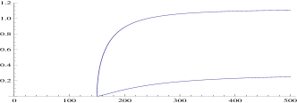
Figure 1: The $\sigma(e^{+}e^{-}\to D^{+}D^{-})/\sigma_{0}$ dependence on $E$ at
$M_{+}=150$ GeV, upper curve – $s_{D}=1/2$, lower curve – $s_{D}=0$.

Table 1: The cross section $\sigma(\mbox{$e^{+}e^{-}\,$}\to D^{+}D^{-})$ for different spins

$E$, GeV	100	250	250	250
$M_{+}$, GeV	80	80	150	200
${s_{D}=0}:$ $\sigma/\sigma_{0}$	0.066	0.245	0.162	0.062
${s_{D}=1/2}:$ $\sigma/\sigma_{0}$	0.84	1.107	1.02	0.82

Total cross section of the $e^{+}e^{-}$ annihilation at ILC for$\sqrt{s}>200$ GeV is $\sim 10\;\sigma_{0}$. The cross section (4) is $\sim\sigma_{0}$. Therefore, the the number of events of considered process is a significant fraction of all the events for $e^{+}e^{-}$ annihilation.

III $\boldsymbol{M_{A}>M_{+}}$, signature

After the production, particles $D^{\pm}$ decay fast to $DW^{\pm}$

$$\mbox{$e^{+}e^{-}\,$}\to D^{+}D^{-}\to DDW^{+}W^{-}\,$$ (6)

with either on shell (real) or off shell $W^{\pm}$, the latter is $q\bar{q}$ pair (dijet) or $\ell\nu$, having the same quantum numbers as $W$ but effective mass $M^{*}<M_{W}$. In both these cases the probability of this decay equals 1. The observable states are decay products of $W$ with large missing transverse energy  $/{E}_{T}$ carried away by the neutral and stable $D$-particle + nothing, the missing mass of particles escaping observation $M(/{E}_{T})$ is large. Therefore, the signatures of the process in the modes, suitable for observation, is

$$\boxed{\mbox{\begin{minipage}{160.43727pt} \centerline{\hbox{A) 2 dijets or}} \centerline{\hbox{B) 1 dijet plus $e$ or $\mu$}} \centerline{\hbox{with large \ $/{E}_{T}$ and large $M(/{E}_{T})$ + {\large\it nothing},}} total energy of each dijet or lepton less \ than $E$. \end{minipage} }}$$ (7)

At $M^{*}>5$ GeV, the branching ratios (BR) for different channels of $W$ decay are practically the same for on shell states PDG and off shell states. In particular, the fraction of events with 2 dijets from hadronic decays of both $W$’s    is $0.676^{2}\approx 0.45$. The fraction of events with 1 dijet from $q\bar{q}$ decay of $W^{\mp}$ plus $\ell=\mu,\,e$ from lepton decay of $W^{\pm}$ is $2\cdot 0.676\cdot 2\cdot(1+0.17)\cdot 0.108\approx 0.33$ (here 0.17 is a fraction of $\mu$ or $e$ from the decay of $\tau$).

At $M^{*}<5$ GeV the BR’s for $e\nu$ and $\mu\nu$ modes increase while dijet degenerates into set of few particles.

IV $\boldsymbol{W}$ energy distribution, $\boldsymbol{M_{A}>M_{+}}$

Let us denote by $M^{*}$ the effective mass of $q\bar{q}$ or $\ell\nu$ pair. At $M_{+}-M_{D}>M_{W}$ we have $M^{*}=M_{W}$ (on shell $W$), at$M_{+}-M_{D}>M_{W}$ possible values of $M^{*}$ are within interval $(0,\,M_{+}-M_{D})$ (off shell $W$). At each value of $M^{*}$ in the rest frame of $D^{\pm}$ we have 2-particle decay

$$\begin{array}[]{c}\!E_{W*}^{r}\!=\!\dfrac{{M_{+}^{2}+M^{*2}-M_{D}^{2}}}{{2M_{+}}},\quad p^{r}_{W*}\!=\!\dfrac{{\Delta(M_{+}^{2},M^{*2},M_{D}^{2})}}{{2M_{+}}},\\[5.69054pt] \Delta(s_{1},s_{2},s_{3})^{2}=s_{1}^{2}+s_{2}^{2}+s_{3}^{2}-2s_{1}s_{2}-2s_{1}s_{3}-2s_{2}s_{3}.\end{array}$$ (8)

Denoting by $\theta$ the $W^{+}$ escape angle in $D^{+}$ rest frame with respect to the direction of $D^{+}$ motion in the Lab system and using $c\equiv\cos\theta$, we find the energy of  $W^{+}$  in the Lab system as $E_{W}^{L}=\gamma_{+}(E_{W*}^{r}+c\beta_{+}p_{W*}^{r})$. Therefore, at given $M^{*}$ the energy $E^{L}_{W}$ of $\ell\nu$ pair or dijet from $W$ decay lies within the interval $\gamma_{+}(E_{W*}^{r}\pm\beta_{+}p_{W*}^{r})$.

At ${M_{+}-M_{D}>M_{W}}$ we deals with on shell $W$, and this equation describes kinematical edges of $W$ energy:

$$E^{L,\pm}_{W,on}\!=\!\gamma_{+}(E_{W}^{r}(M_{W})\!\pm\!\beta_{+}p^{r}_{W}(M_{W})).$$ (9)

At ${M_{+}-M_{D}<M_{W}}$ similar edges are different for each value of $M^{*}$. In particular, at the highest value $M^{*}=M_{+}-M_{D}$ we have $p_{W}^{r}=0$, and interval, similar to (9) reduces to a point, where entire $W$ energy distribution has maximum (peak)

$$E^{L}_{W,p}\equiv E^{L,\pm}_{W}|_{(M^{*}=M_{+}-M_{D})}=E\left(1-\dfrac{{M_{D}}}{{M_{+}}}\right).$$ (10)

Absolute upper and lower bounds on the energy distribution of the muons are achieved at $M^{*}=0$, they are

$$E^{L,\pm}_{W,off}=E\,\dfrac{{1\pm\beta_{+}}}{{2}}\left(1-\dfrac{{M_{D}^{2}}}{{M_{+}^{2}}}\right)\;.$$ (11)

V Single lepton energy distribution in $\boldsymbol{\mbox{$e^{+}e^{-}\,$}\to D^{+}D^{-}\to DDW^{+}W^{-}\to DDq\bar{q}\,\ell\nu}$

The lepton energy ${\varepsilon}$ is measurable with high accuracy. Therefore it is useful to study the energy distribution $d\sigma_{0}^{\mu}({\varepsilon}|M_{+},\,M_{D})/d{\varepsilon}$ for the events with signature (7B) more attentively. We find that this distribution has singular points which positions are model independent. We consider, for   definiteness, $\ell=\mu^{-}$, neglect the muon mass and limit ourself in this section to the case $M_{A}>M_{+}$.

a) If ${M_{+}-M_{D}>M_{W}}$, the muon energy and momentum in the rest frame of $W$ are $M_{W}/2$. In the Lab system for $W$ with some energy $E_{W}^{L}$ the $\gamma$-factor and the velocity of $W$ are$\gamma_{WL}=E_{W}^{L}/M_{W}$ and $\beta_{WL}\equiv\sqrt{1-\gamma_{WL}^{-2}}$. Just as above, denoting by $\theta_{1}$ the escape angle of $\mu$ relative to the direction of the $W$ in the Lab system and $c_{1}=\cos\theta_{1}$, we find that in the Lab system the muon energy ${\varepsilon}=\gamma_{WL}\left(1+c_{1}\beta_{WL}\right)(M_{W}/2)$. Therefore

$${\varepsilon}^{+}(E^{L}_{W})\geqslant{\varepsilon}\geqslant{\varepsilon}^{-}(E^{L}_{W})\equiv M_{W}^{2}/\left(4{\varepsilon}^{+}(E^{L}_{W})\right),$$

where ${\varepsilon}^{+}(E^{L}_{W})=E_{W}^{L}\dfrac{{1+\beta_{WL}}}{{2}}=\dfrac{{E_{W}^{L}+\sqrt{(E_{W}^{L})^{2}-M_{W}^{2}}}}{{2}}$.

The interval, corresponding to energy $E_{1W}^{L}<E_{W}^{L}$, is located entirely within the interval, correspondent to energy $E_{W}^{L}$. Therefore, all muon energies lie within the interval determined by the highest value of $W$ energy:

$$\begin{array}[]{c}{\varepsilon}^{+}\geqslant{\varepsilon}\geqslant{\varepsilon}^{-}\equiv\dfrac{{M_{W}^{2}}}{{4{\varepsilon}^{+}}},\;\;where\\[5.69054pt] {\varepsilon}^{+}\equiv{\varepsilon}^{+}(E^{L,+}_{W,on})=\dfrac{{E^{L,+}_{W,on}+\sqrt{(E^{L,+}_{W,on})^{2}-M_{W}^{2}}}}{{2}}\,.\end{array}$$ (12)

Contributions of $W$ with intermediate energies are summarized in the entire distribution of muons in the energy, and it increases monotonically from the outer limits to kinks at energies ${\varepsilon}^{\pm}_{k}$, corresponding to the lowest energy $E^{L,-}_{W,on}$ of the $W$ boson:

$${\varepsilon}^{\pm}_{k}\equiv{\varepsilon}^{+}(E^{L,-}_{W,on})=\dfrac{{E^{L,-}_{W,on}\pm\sqrt{(E^{L,-}_{W,on})^{2}-M_{W}^{2}}}}{{2}}\,.$$ (13)

Between these kinks $d^{2}N/d{\varepsilon}^{2}\approx 0$. The energy distribution of muons for the case of matrix element, independent on $\theta_{1}$, is shown in Fig. 2 – up. Calculations for separate models (where angular dependence exists) demonstrate variation in details of shape of these curves but the position of kinks is fixed GKr .

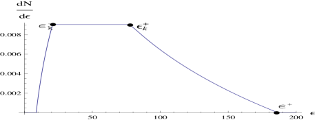
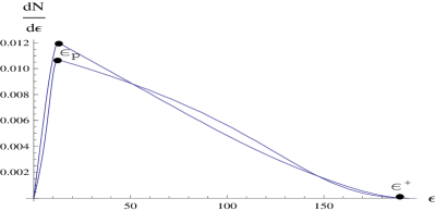
Figure 2: The normalized distributions $dN/d\epsilon\equiv(1/\sigma)d\sigma/d\epsilon$ for $M_{+}=150$ GeV (on shell $W$) – upper plot, for $M_{+}=120$ GeV (off shell $W$) – lower plot, $E=250$ GeV. At lower plot upper peak – for $s_{D}=0$, lower peak – for $s_{D}=1/2$.

b) If ${M_{+}-M_{D}<M_{W}}$, the $D^{\pm}$ decays to $(D+W^{*})$ where $W^{*}$ is off shell $W$ with effective mass $M^{*}\leqslant M_{+}-M_{D}$. The calculations, similar to above, for each $M^{*}$ shows  that the muon energies are within the interval, appearing at $M^{*}=0$:

$$\left\{{\varepsilon}^{-}=0;\;{\varepsilon}^{+}=E\,\dfrac{{1+\beta_{+}}}{{2}}\left(1-\dfrac{{M_{D}^{2}}}{{M_{+}^{2}}}\right)\equiv E^{L,+}_{W,off}\,\right\}.$$ (14)

Similarly to the preceding discussion, the increase of $M^{*}$ shifts the interval boundaries inside. Therefore, the muon energy distribution increases monotonically from outer bounds up to the maximum (peak) at $M^{*}=M_{+}-M_{D}$ (cf. (10)):

$${\varepsilon}_{p}=E\dfrac{{1+\beta_{+}}}{{2}}\left(1-\dfrac{{M_{D}}}{{M_{+}}}\right).$$ (15)

To get an idea about the shape of the peak, one should use the distribution of $W^{*}$’s (dijets or $\ell\nu$ pairs) over the effective masses $M^{*}$. It is given by the spin dependent factor $R_{s_{D}}p^{*}dM^{*2}$:

$$\begin{array}[]{c}R_{0}=\dfrac{{p^{*2}}}{{(M_{W}^{2}-M^{*2})^{2}}}\,,\\ \!\!\!\!R_{1/2}\!=\!\dfrac{{(M_{+}^{2}\!+\!M_{D}^{2}\!-\!M^{*2})(2M_{W}^{2}\!+\!M_{+}^{2}\!+\!M_{D}^{2})\!-\!4M_{+}^{2}M_{D}^{2}}}{{(M_{W}^{2}-M^{*2})^{2}M_{W}^{2}}}.\end{array}$$ (16)

The density of muon states in energy $dN/d{\varepsilon}$ is calculated by convolution of kinematically defined distribution with distribution (16). Neglecting the dependence of the matrix element of the angle, we obtain result in form of Fig. 2-down. One can see that the discussed peak is sharp enough for both values of spin $s_{D}=0$ and $1/2$.

Characteristic values for singular point (kink and peak) energies in these distributions (together with similar points for energy distributions of $W$ (dijets)) are given in the table 2 .

Table 2: The singular point energies of lepton and $q\bar{q}$ dijet in
$\mbox{$e^{+}e^{-}\,$}\to D^{+}D^{-}\to DDq\bar{q}\ell\nu$ (in GeV) at $M_{D}=50$ GeV.

$E$	$M_{+}$	${\varepsilon}^{+}$	${\varepsilon}^{+}_{k}$	${\varepsilon}_{p}$	$E^{L}_{Wp}$	$E^{L,+}_{W}$
250	150	186.3	77.8	-	-	195.4
250	200	184.9	46.3	-	-	193.6
250	80	148.3	-	91.3	93.75	148.3
100	80	78	-	30	37.5	78

The cascade $\boldsymbol{D^{+}\to DW^{+}\to D\tau^{+}\nu\to D\mu^{+}\nu\nu\nu}$ modifies spectra under discussion. The energy distribution of $\tau$, produced in the decay $W\to\tau\nu$, is the same as that for $\mu$ or $e$, discussed above (with accuracy $M_{\tau}/M_{W}$ or $M_{\tau}/M^{*}$). After its production, $\tau$ decays to $\mu\nu\nu$ in 17 % cases (the same for decay to $e\nu\nu$). These muons are added to the above discussed.

In the $\tau$ rest frame the energy of muon $E_{\mu}^{\tau}=y\,M_{\tau}/2$ with $y\leqslant 1$. The energy spectrum of muons is $dN/dy=2(3-2y)y^{2}$ (see textbooks). This spectrum and distributions, obtained above, are converted into the energy distribution of these muons in the Lab system. Two features of this contribution are clear on the qualitative level

A) This contribution is shifted strong to the soft part of energy spectrum.

B) This contribution has no singular points with jump of derivative in ${\varepsilon}$.

The resulted muon energy distribution is similar to that without $\tau$ contribution, Fig. 2. This contribution does not change the upper end point of the energy distribution of the muons ${\varepsilon}^{+}$ (12), (14). Numerical examples GKr show that the discussed correction shifts positions of kinks or peak in the muon energy distributions by less than 1 GeV, i.e. negligibly.

VI Case $\boldsymbol{M_{+}>M_{A}}$

For the main process $\mbox{$e^{+}e^{-}\,$}\to D^{+}D^{-}$ at $M_{+}>M_{A}$ one more decay become also possible, $\boldsymbol{D^{\pm}\to D^{A}W^{\pm}\to DZW^{\pm}}$. Total probability of decays $D^{+}$ to $D^{A}W^{+}$ and $DW^{+}$ equals 1. The decay $D^{\pm}\to D^{A}W^{\pm}$ is described by the same equation as $D^{\pm}\to DW^{\pm}$, but with another kinematical factors since $M_{A}>M_{D}$. The probability of this new decay is lower than that without $D^{A}$ due to smaller final phase space volume, i.e. $B=BR(D^{+}\to D^{A}W^{+})<0.5$.

In the same manner as above, particle $D^{A}$ decays fast to $DZ$ and we deals with cascades

$e^{+}e^{-}\to D^{+}D^{-}\to DW^{+}D^{A}W^{-}\to DDW^{+}W^{-}Z$, etc.

Now signature of processes $e^{+}e^{-}\to D^{+}D^{-}$ in the modes, suitable for observation, contains both (7) and

$$\boxed{\mbox{\begin{minipage}{177.78578pt} 3 or 4 dijets, or less dijets plus 1 to 5 leptons with large $/{E}_{T}$ and large $M(/{E}_{T})$ + {\large\it nothing}. \end{minipage} }}$$ (17)

Note that 20% of final states of $Z$ decay are invisible ($\nu\bar{\nu}$ final states). We denote these states as $Z_{n}$.

Let us consider in more detail final states with signature (7B) (observed state: 1 dijet $+\mu^{-}$ +nothing). This state can be obtained from two group of channels with different mechanism of cascades $D^{-}\to D\mu^{-}+\ldots$   and all possible channels for decay $D^{+}$:
1) Channels where $D^{-}$ decays to $DW^{-}\to D\mu^{-}\nu$. The energy distribution of $\mu^{-}$ in these channels reproduces that, obtained for the case $M_{A}>M_{+}$ (Sect. V), that is$(1-B)d\sigma_{0}^{\mu}({\varepsilon}|M_{+},\,M_{D})/d{\varepsilon}$. Here $d\sigma_{0}^{\mu}({\varepsilon}|M_{+},\,M_{D})/d{\varepsilon}$ is energy distribution obtained for the case $M_{A}>M_{+}$, we have written explicitly the arguments indicating mass of the initial and final $D$-particles.
2) Channels where $D^{-}$ decays to $D^{A}W^{-}\to DZ_{n}\mu^{-}\nu$. Since couplings $D^{-}DW^{-}$ and $D^{-}D^{A}W^{-}$ differ by phase factor only, the energy distribution of $\mu^{-}$ in these channels is described by the same dependence $d\sigma_{0}$ but with the change $M_{D}\to M_{A}$, the corresponding contribution to the entire energy distribution is $0.2Bd\sigma_{0}^{\mu}({\varepsilon}|M_{+},\,M_{A})/d{\varepsilon}$. For brevity we will write $d\sigma_{0}^{\mu}({\varepsilon}|M_{+},\,M_{D})\to d\sigma^{\mu}_{W}$ and $d\sigma_{0}^{\mu}({\varepsilon}|M_{+},\,M_{A})\to d\sigma^{\mu}_{WZn}$. The resulting energy distribution is

$$d\sigma_{tot}^{\mu}/d{\varepsilon}=(1-B)d\sigma_{W}^{\mu}/d{\varepsilon}+0.2Bd\sigma_{WZn}^{\mu}/d{\varepsilon}\,.$$ (18)

The shape of distribution $d\sigma_{WZn}^{\mu}/d{\varepsilon}$ is similar to that for $d\sigma_{W}^{\mu}/d{\varepsilon}$ (Sect. V) but with another positions of kinks and (or) peak. Since $M_{A}>M_{D}$, these new kinks and (or) peak are situated below similar positions for $d\sigma_{W}^{\mu}/d{\varepsilon}$. Since this contribution is much smaller than the main contribution $d\sigma_{W}^{\mu}/d{\varepsilon}$ (with overall ratio $0.2B/(1-B)$ at $B<0.5$), it results in only weak change of entire energy distribution as compare with distributions in Sect. V. The opportunity to extract from the data new singularities, related to $d\sigma_{WZn}^{\mu}/d{\varepsilon}$, demands separate study.

VII Discovery, measuring of masses and spin

Discovery. The observation of events with signature (7), (17) will be a clear signal of candidates for DM particles. The process with signature (17) can take place only simultaneously with processes $\mbox{$e^{+}e^{-}\,$}\to DDZ$ with signature (20).

Masses $\boldsymbol{M_{+}}$ and $\boldsymbol{M_{D}}$ can be determined from singular points of the energy distribution of the leptons in the final state $q{\bar{q}}\ell$ + nothing by summing contributions from $e$ and $\mu$. With anticipated annual luminosity integral $\cal L$ for the ILC project WILC ${\cal L}\sigma_{0}\sim 10^{5}$ the 1-year number of events of this type will be $\sim(1\div 3)\cdot 10^{4}$, depending on masses and spin $s_{D}$.

M1) If $D^{A}$ particle is absent or at $M_{+}<M_{A}$, the results of Sect. V describe the energy distributions completely. The shape of energy distribution of leptons (with one peak or two kinks) allows to determine what case is realized,$M_{+}-M_{D}>M_{W}$ or $M_{+}-M_{D}<M_{W}$. At $M_{+}-M_{D}>M_{W}$ the position of upper edge of the muon energy ${\varepsilon}^{+}$ (12) and one kink, e.g. ${\varepsilon}^{+}_{k}$ (13) give us two equations necessary for determination of $M_{D}$ and $M_{+}$. At $M_{+}-M_{D}<M_{W}$ two similar equations are given by the position of upper end point of the muon energy ${\varepsilon}^{+}$ (14) and peak ${\varepsilon}_{p}$ (15).

The singular points of dijet energy distribution can be also used for measuring on masses.

At $M_{+}-M_{D}>M_{W}$ the upper edges of dijet energy distribution $E^{L}_{W}$ and muon energy distribution ${\varepsilon}^{+}$ contains identical information, since $E^{L,+}_{W}\!\!=\!\!{\varepsilon}^{+}\!\!+\!M_{W}^{2}/4{\varepsilon}^{+}$ (cf. (9), (12)). In this case results of measuring $E^{L,+}_{W}$ and ${\varepsilon}^{+}$ supplement each other.

At $M_{+}-M_{D}<M_{W}$ we have $E^{L,+}_{W}={\varepsilon}^{+}$ at $M_{+}-M_{D}<M_{W}$ (cf. (11), (14)). In this case measuring of $E^{L,+}_{W}$ meet additional difficulties since this upper edge is given by values of $M^{*}$, close to 0, when dijet is degenerated into 2-3 pions. The position of peak in the dijet energy distribution $E^{L}_{Wp}$ looks useful since ${\varepsilon}_{p}/E^{L}_{Wp}=(1+\beta_{+})/2$ (cf. (10), (15)). However position of this peak in the dijet distribution is smeared by an uncertainty in the measurement of the energy of individual jets.

M2) For the case $M_{+}>M_{A}$ the entire energy distribution of muons in the observed state $\mu$ +1 dijet + nothing was described in Sect. VI. As it was mention there, taking into account a new decay channel $D^{-}\to D^{A}W^{-}\to DZ_{n}\mu^{-}\nu$ changes the position of the main singularities in the muon energy spectrum only a little. Therefore the above mentioned procedure for finding $M_{+}$ and $M_{D}$ can be used in this case as well.

Note that in the case $M_{A}\approx M_{D}$ distributions $d\sigma_{WZn}^{\mu}/d{\varepsilon}$ and $d\sigma_{W}^{\mu}/d{\varepsilon}$ are close to each other, and discussed procedure describes ”degenerated” quantity $M_{A}\approx M_{D}$. In the opposite degenerate case $M_{+}\approx M_{A}$ quantity $B\ll 1$, and influence of intermediate $D_{A}$ state on the result is negligible.

M3) At $M_{A}+M_{D}<2E$ the process

$$e^{+}e^{-}\to Z\to DD^{A}\to DDZ$$ (19)

becomes possible with clear signature

$$\boxed{\mbox{\begin{minipage}{177.78578pt} The dilepton (\mbox{$e^{+}e^{-}\,$}\ or $\mu^{+}\mu^{-}$ \ pair) or quark dijet with large \ $/{E}_{T}$ and large $M(/{E}_{T})$ + {\large\it nothing}. The effective mass of this dilepton or dijet is either $M_{Z}$ or lower than $M_{Z}$. \end{minipage} }}$$ (20)

The cross section of this process is also $\sim\sigma_{0}$ but it is smaller than that for production $D^{+}D^{-}$ (4) with smaller BR for lepton mode. Moreover, the value of this cross section is highly model dependent. With annual luminosity (5), the 1-year number of events of this type will be $\lesssim(3\div 15)\cdot 10^{2}$ (depending on masses, spin $s_{D}$ and details of the model) Gin10 .

The calculations similar to those for $W$ energy distribution for process (6) allow to obtain kinematical edges of the energy distribution of dilepton for each value of its effective masses like (9)-(11). Measuring these edges gives two equations for finding $M_{A}$ and $M_{D}$. (If $M_{A}-M_{D}<M_{Z}$, this procedure must be performed separately for each value of the effective mass of dilepton.) Gin10 , WILC , kinemLHC .

Spin of $\boldsymbol{D}$-particles $\boldsymbol{s_{D}}$. The cross section of the process $e^{+}e^{-}\to D^{+}D^{-}$ is obtained by summation over all processes with signature (7), (17) taking into account the known BR’s for $W$ decay.

When masses $M_{+}$ become known, the cross section of the process $e^{+}e^{-}\to D^{+}D^{-}$ is calculated easily for each value of spin (4). The main part of the $\sigma(e^{+}e^{-}\to D^{+}D^{-})$ is given by model independent QED contribution of photon exchange, whereas the model dependent contribution of $Z$ exchange at $\sqrt{s}>200$ GeV contributes less than 30%. For identical masses $\sigma(S_{D}=1/2)>4\sigma(s_{D}=0)$ (cf. table 1 and Fig. 1 for examples). This strong difference in the cross sections for different $s_{D}$ allows to determine spin of $D$ particle even at low accuracy in the measuring of cross section.

The similar procedure for the process $\mbox{$e^{+}e^{-}\,$}\to DD^{A}$ cannot be developed in the model independent way due to the strong model dependence of cross section.

VIII Background

$\boldsymbol{BW1}$. The process $\boldsymbol{\mbox{$e^{+}e^{-}\,$}\to W^{+}W^{-}}$ gives the same final state as our process (7). However, many of its features are not permitted in signature (7).
(a) Energy of each dijet equals $E$.
(b) For the dijet+dijet observable state the observed   $/{E}_{T}$ is low (in an ideal case  $/{E}_{T}=0$).
(c) For the dijet +lepton state the missing mass $M(/{E}_{T})$ is low (in an ideal case $M(/{E}_{T})=0$.
These differences allow to exclude process $BW1$ from the analysis with a good confidence by application of suitable cuts.

$\boldsymbol{BW2}$. $\boldsymbol{\mbox{$e^{+}e^{-}\,$}\to DD^{A}\to DD^{+}W^{-}\to DDW^{+}W^{-}}$ at $\boldsymbol{M_{A}>M_{+}}$. If $\sigma(\mbox{$e^{+}e^{-}\,$}\to DD^{A})$ is not small at given $\sqrt{s}$, this fact will be seen via observation of the process $\mbox{$e^{+}e^{-}\,$}\to DDZ$ (20). The cross section $\sigma(BW2)<\sigma(\mbox{$e^{+}e^{-}\,$}\to DDZ)$, i.e. it is much less than $\sigma(\mbox{$e^{+}e^{-}\,$}\to D^{+}D^{-}\to DDW^{+}W^{-})$. Its contribution may be reduced additionally by application of cuts taking into account the following points.
(a) In the process $BW2$ all recorded particles move in one hemisphere in contrast with process (7), where they move in two opposite hemispheres.
(b) In the process $BW2$ total energies of lepton and jet are typically very different in contrast to the process $\mbox{$e^{+}e^{-}\,$}\to W^{+}W^{-}\to DDW^{+}W^{-}$ where these energies are close to each other.

$\boldsymbol{BW3}$. In the SM processes with observed state, satisfying criterion (7), large $/{E}_{T}$ is carried away by additional neutrinos. The corresponding cross section is at least one electroweak coupling constant squared $g^{2}/4\pi$ or $g^{\prime 2}/4\pi$ smaller than $\sigma_{0}$, with $g^{2}/4\pi\sim g^{\prime 2}/4\pi\sim\alpha$. Therefore, the cross sections for these background processes are by about one or two orders of magnitude smaller than the cross section of the process under discussion.

We discuss also briefly background processes for $\boldsymbol{e^{+}e^{-}\to DD^{A}\to DD\ell^{+}\ell^{-}}$. These processes are subdivided into 3 groups.

BZ1. $\mbox{$e^{+}e^{-}\,$}\to ZZ_{n}$. At first sight, this process can mimic the process $\mbox{$e^{+}e^{-}\,$}\to DDZ$. However, the lepton or quark pairs in the process BZ1 have the same energy $E$ as the colliding electrons. Therefore the criterion (20) excludes such events from the analysis.

The cross section $\sigma(\mbox{$e^{+}e^{-}\,$}\to ZZ_{n})\sim 0.2\cdot 3r_{Z}\sigma_{0}\ln(s/M_{Z}^{2})$. The variants of this process with off shell $Z$, giving another effective mass of observed dijet or dilepton and, respectively, another values of their energy, has cross section which is smaller by factor $\sim\alpha$.

BZ2. Processes with independent production of separate:
(BZ2.1) $\mbox{$e^{+}e^{-}\,$}\to DDZ\to DD\tau^{+}\tau^{-}\to DD\,\ell_{1}^{+}\ell_{2}^{-}+\nu^{\prime}s$,
(BZ2.2) $\mbox{$e^{+}e^{-}\,$}\to DD^{A}\to DDW^{+}W^{-}\to DD\ell_{1}\bar{\ell}_{2}\nu\bar{\nu}$,
(BZ2.3) $\mbox{$e^{+}e^{-}\,$}\to D^{+}D^{-}\to DDWW\to DD\ell_{1}\bar{\ell}_{2}\nu\bar{\nu}$,
(BZ2.4) $\mbox{$e^{+}e^{-}\,$}\to W^{+}W^{-}\to\ell_{1}\bar{\ell}_{2}\nu\bar{\nu}$.
In these processes $e^{+}e^{-}\,$, $\mu^{+}\mu^{-}$, $e^{-}\mu^{+}$ and $e^{+}\mu^{-}$ pairs are produced with identical probability and identical distributions. Hence,

$$\begin{array}[]{c}\mbox{\it the subtraction from the $\mbox{$e^{+}e^{-}\,$}$ and $\mu^{+}\mu^{-}$ data }\\ \mbox{\it the measured distributions of \ $e^{-}\mu^{+}$ and \ $e^{+}\mu^{-}$}\end{array}$$ (21)

eliminates contribution of these processes from the energy distributions under interest. This procedure does not implement substantial inaccuracies since cross sections of these processes after suitable cuts will be small enough.

The cross sections of processes (BZ2.1), (BZ2.2) are small in comparison with that for $e^{+}e^{-}\to DD\mu^{+}\mu^{-}$. In the process (BZ2.3) leptons are flying in the opposite hemisphere, in contrast to the process under study $\mbox{$e^{+}e^{-}\,$}\to DDZ\to DD\mu^{+}\mu^{-}$, where the leptons are flying in the same hemisphere The cross section of the process (BZ2.4) is basically large. The application of cuts $E_{\ell\bar{\ell}}<E$, $M_{\ell\bar{\ell}}\leqslant M_{Z}$ leaves less than $(M_{Z}^{2}/s)^{2}\ln(s/M_{Z}^{2})$ part of the cross section. The obtained quantity becomes smaller than that for the signal.

BZ3. In the SM processes with observed state (20), the large $/{E}_{T}$ is carried away by additional neutrino(s). The magnitude of corresponding cross sections are at least by one electroweak coupling constant squared $g^{2}/4\pi$ or $g^{\prime 2}/4\pi$ less than $\sigma_{0}$, with $g^{2}/4\pi\sim g^{\prime 2}/4\pi\sim\alpha$. Therefore, the cross sections of these processes are at least one order of magnitude smaller than the cross section for the signal process.

Some limitation.

In the real analysis, the energy spectra under discussion will be smeared due to initial state radiation and beamstrahlung.

This work was supported in part by grants RFBR 11-02-00242, NSh-3802.2012.2, Program of Dept. of Phys. Sc. RAS and SB RAS ”Studies of Higgs boson and exotic particles at LHC” and Polish Ministry of Science and Higher Education Grant N N202 230337. I am thankful A.E. Bondar, A.G. Grozin, I.P. Ivanov, D.Yu. Ivanov, D.I. Kazakov, J. Kalinowski, K.A. Kanishev, P.A. Krachkov and V.G. Serbo for discussions.

References

- (1) For example, D. Hooper. hep-ph/0901.4090; M. Maniatis. hep-ph/0906.0777; D.I. Kazakov, hep-ph/1010.5419; J. Ellis. hep-ph/1011.0077.
- (2) N. G. Deshpande, E. Ma, Phys. Rev. D 18 (1978) 2574; R. Barbieri, L. J. Hall, V. S. Rychkov, Phys. Rev. D 74 (2006) 015007, hep-ph/0603188; Ginzburg I.F., Kanishev K.A., Krawczyk M., Sokołowska D. Phys. Rev. D 82 (2010) 123533; hep-ph/1009.4593
- (3) E. M. Dolle and S. Su, Phys. Rev. D 80 (2009) 055012 [arXiv:0906.1609 [hep-ph]]; E. Dolle, X. Miao, S. Su and B. Thomas, Phys. Rev. D 81, 035003 (2010) [arXiv:0909.3094 [hep-ph]]; L. Lopez Honorez, E. Nezri, J. F. Oliver and M. H. G. Tytgat, JCAP 0702 (2007) 028 [arXiv:hep-ph/0612275]; C. Arina, F. S. Ling and M. H. G. Tytgat, E. Nezri, M. H. G. Tytgat and G. Vertongen, JCAP 0904 (2009) 014 [arXiv:0901.2556 [hep-ph]]; S. Andreas, T. Hambye and M. H. G. Tytgat, JCAP 0810 (2008) 034 [arXiv:0808.0255 [hep-ph]]; L. L. Honorez and C. E. Yaguna, arXiv:1003.3125
- (4) Particle Data Group. Journ. of Phys. G 37 #7A (2010) 075021.
- (5) E. Lundstrom, M. Gustafsson and J. Edsjo, Phys. Rev. D 79 (2009) 035013 [arXiv:0810.3924 [hep-ph]].
- (6) R.D. Heuer et al. TESLA Technical Design Report, DESY 2001-011, TESLA Report 2001-23, TESLA FEL 2001-05 (2001).
- (7) Asano M., Fujii K., Hundi R. S., Itoh H., Matsumoto S., Okada N., Saito T., Suehara T., Takubo Y., Yamamoto H. Phys. Rev. D 84, 115003 (2011), arXiv:1007.2636; 1106.1932 [hep-ph];
- (8) See e.g. A.J. Barr, K. Road. J.Phys. G37 123001 (2010), arXiv:1004.2732 [hep-ph] K. Agashe, D. Kim, M. Toharia, D.G.E. Walker. Phys. Rev. D 82, 015007 (2010) arXiv:1003.0899 [hep-ph]
- (9) I.F. Ginzburg, P.A. Krachkov, in preparation
- (10) I.F. Ginzburg, arXiv:1010.5579 [hep-ph]