Advances in mean-field dynamo theories

Abstract

We give a short introduction to the subject and review advances in understanding the basic ingredients of the mean-field dynamo theory. The discussion includes the recent analytic and numerical work in developments for the mean electromotive force of the turbulent flows and magnetic field, the nonlinear effects of the magnetic helicity, the non-local generation effects in the dynamo. We give an example of the mean-field solar dynamo model that incorporates the fairly complete expressions for the mean-electromotive force, the subsurface shear layer and the conservation of the total helicity. The model is used to shed light on the issues in the solar dynamo and on the future development of this field of research.

Is dynamo in tachocline or in convection zone?
That is the question!
Whether ’tis nobler in the mind to fit
Parameters of model to reproduce the observations
Or to take the theory and direct simulations
And try to answer basic questions:
Why magnetic field is generated?
And why it drifts equatorward in course of solar cycle?
’tis a consummation devotely to be wished! take-off Shakespeare

1 Introduction

The mean-field magnetohydrodynamic presents one of the most powerful tools for exploring the nature of the large-scale magnetic activity in cosmic bodies (Moffatt 1978; Parker 1979; Krause & Rädler 1980). It is widely believed that magnetic field generation there is governed by interplay between turbulent motions of electrically conductive fluids and global rotation. The dynamo theory studies the evolution of the magnetic field which is govern by the induction equation:

$$\frac{\partial\mathbf{B}}{\partial t}=\nabla\times\left(\mathbf{U\times B}-\eta\nabla\times\mathbf{B}\right),$$

where $\mathbf{B}$ is the magnetic field induction vector, $\mathbf{U}$ is the velocity field of the plasma and $\eta$ is the molecular magnetic diffusivity.

2 The mean electromotive force

The aim of this section is to briefly outline the basic equations and methods of the mean-field magnetohydrodynamic (MHD). The general framework of the mean-field MHD can be introduced as follows. In the turbulent media, it is feasible to decompose the fields on the mean and fluctuated parts, e.g., $\mathbf{B}=\overline{\mathbf{B}}+\mathbf{b},\,\mathbf{U}=\mathbf{\overline{\mathbf{U}}}+\mathbf{u}$. Hereafter, everywhere, we use the small letters for the fluctuating part of the fields and capital letters with a bar above for the mean fields. Let’s define the typical spatial, $L,\ell$ , and temporal, $T,\tau_{c}$, variation scales for the mean and the fluctuated parts of the fields. It is a typical situation for the astrophysical system when the flows and magnetic fields are strongly turbulent, i.e., the Strouhal number $St={\displaystyle\frac{u\tau_{c}}{\ell}\sim 1}$ and the Reynolds number $R_{e}={\displaystyle\frac{u\ell}{\nu}}\gg 1$, where $\nu$ is the molecular viscosity. Assuming the validity of the Reynolds rules (Monin & Yaglom 1975) and averaging the induction equation over the ensemble of the fluctuating fields we get the mean-field dynamo equation:

$$\frac{\partial\overline{\mathbf{B}}}{\partial t}=\nabla\times\left(\mathbf{\overline{U}\times}\overline{\mathbf{B}}+\boldsymbol{\mathcal{E}}\right),\,\,\,\boldsymbol{\mathcal{E}}\mathbf{=}\overline{\mathbf{u}\times\mathbf{b}}$$ (1)

There are two contributions here. In a perfectly conducting fluid, when the magnetic Reynolds number $R_{m}={\displaystyle\frac{u\ell}{\eta}}\gg 1$, the magnetic flux is frozen into fluid. Then, the first term can be interpreted as the defection, stretching and compression (or expansion) of the magnetic field by mean flow, because of $\mathbf{\nabla\times\left(\overline{U}\times\overline{\mathbf{B}}\right)}=-\left(\overline{\mathbf{U}}\cdot\nabla\right)\mathbf{\overline{B}}+\left(\mathbf{\overline{B}}\cdot\nabla\right)\mathbf{\overline{U}}-\overline{\mathbf{B}}\left(\nabla\cdot\overline{\mathbf{U}}\right)$. The effect of the turbulence is represented by the mean electromotive force $\boldsymbol{\mathcal{E}}\mathbf{=}\overline{\mathbf{u}\times\mathbf{b}}$. It is possible to analyze the general structure of the $\boldsymbol{\mathcal{E}}$ using the assumption about the scale separation in the turbulence $L,T\gg\ell,\tau_{c}$ and the transformation symmetry properties of the basic physical quantities (Rädler 1969; Krause & Rädler 1980; Brandenburg et al. 2012):

$$\boldsymbol{\mathcal{E}}=\left(\hat{\mathbf{\alpha}}+\hat{\mathbf{\gamma}}\right)\circ\overline{\mathbf{B}}-\hat{\eta}\circ\left(\nabla\times\overline{\mathbf{B}}\right)+\hat{\kappa}\circ\left(\boldsymbol{\nabla}\overline{\mathbf{B}}\right)+o\left(\frac{\ell}{L}\right),$$ (2)

where $\left(\boldsymbol{\nabla}\overline{\mathbf{B}}\right)_{\{i,j\}}=\frac{1}{2}\left(\nabla_{i}\overline{B}_{j}+\nabla_{j}\overline{B}_{i}\right)$, the kinetic coefficients $\hat{\mathbf{\alpha}},\hat{\mathbf{\gamma}},\hat{\eta},\hat{\kappa}$ are tensors and the symbol $\circ$ marks the tensor product.

The kinetic coefficients may depend on the global factors, which determine the large-scale properties of the astrophysical system, for example, the global rotation angular velocity $\boldsymbol{\Omega}$, the large-scale vorticity $\mathbf{W}=\boldsymbol{\nabla}\times\overline{\mathbf{U}}$, the stratification parameters like $\boldsymbol{\nabla}\overline{\rho}$, $\boldsymbol{\nabla}\overline{\mathbf{u}^{2}}$, and the global constraints, like, magnetic helicity conservation. For the simplest case when $\hat{\alpha}\sim\alpha_{0}\delta_{ij}$, $\hat{\eta}\sim\eta_{T}\delta_{ij}$ and $\hat{\gamma}\sim-\varepsilon_{ijn}\overline{V}_{n}^{(p)}$ and $\hat{\kappa}$ is neglected we get(Krause & Rädler 1980):

$$\mathcal{E}_{i}=\alpha_{0}B_{i}+\left(\mathbf{\overline{V}}^{(p)}\times\overline{\mathbf{B}}\right)-\eta_{T}\left(\nabla\times\overline{\mathbf{B}}\right),$$ (3)

where $\alpha_{0}$ is the magnitude of the $\alpha$ effect, $\overline{\mathbf{V}}^{(p)}$ is the turbulent pumping velocity and $\eta_{T}$ is the isotropic turbulent diffusivity.

To calculate the kinetic coefficients we use the equations which govern the evolution of the fluctuating magnetic and velocity fields. For example, taking into account the effects of the global rotation and shear for the incompressible turbulent flows, we get the equations as follows (see, e.g., Rädler et al. 2003; Brandenburg & Subramanian 2005)

$$\frac{\partial\mathbf{b}}{\partial t} = \nabla\times\left(\mathbf{u}\times\mathbf{\overline{B}}+\mathbf{\overline{U}}\times\mathbf{b}\right)+\eta\nabla^{2}\mathbf{b}+\mathfrak{G},$$ (4)

$$\frac{\partial u_{i}}{\partial t}+2\left(\mathbf{\Omega}\times\mathbf{u}\right)_{i} = -\nabla_{i}\left(p+\frac{\left(\mathbf{b\cdot}\overline{\mathbf{U}}\right)}{\mu}\right)+\nu\Delta u_{i}$$

$$+ \frac{1}{\mu}\nabla_{j}\left(\overline{B}_{j}b_{i}+\overline{B}_{i}b_{j}\right)-\nabla_{j}\left(\overline{U}_{j}u_{i}+\overline{U}_{i}u_{j}\right)+f_{i}+\mathfrak{F}_{i},$$

where $\mathfrak{G},\mathfrak{F}$ stand for the nonlinear contributions of fluctuating fields, $p$ is the fluctuating pressure, $\mathbf{\Omega}$ is the angular velocity responsible for the Coriolis force, $\mathbf{f}$ is the random force driving the turbulence.

Using Eqs(4,2), $\boldsymbol{\mathcal{E}}$ can be calculated analytically by different ways. The first-order smoothing, also known as the second order correlation approximation (SOCA) uses the condition $\min\left(Rm,St\right)\ll 1$ and neglect the nonlinear contributions in Eqs(4,2) (Moffatt 1978; Krause & Rädler 1980). The $\tau$-approximations was introduced to take into account the nonlinear effects of the second order correlations. It is claimed to be valid for $Rm,Re\gg 1$ and for the developed turbulence in equilibrium state. In this case we solve the equations for the second order correlations and replace the third-order correlations of the fluctuating parameters, with the second order relaxation terms (see details in Kleeorin et al. 1996; Blackman & Field 2002; Rädler et al. 2003; Brandenburg & Subramanian 2005). This approximation is based on questionable assumptions ( Rädler & Rheinhardt 2007), e.g., it is assumed that the second-order correlations do not vary significantly on the time scale of $\tau_{c}$. This assumption is consistent with scale separation between the mean and fluctuating quantities in the mean-field magnetohydrodynamic. The reader can find a comprehensive discussion of the $\tau$ -approximation in the above cited papers.

The path integral approach use the ideas from the stochastic calculus (Dittrich et al. 1984; Zel’dovich et al. 1984). This approach is valid for the case $Re\gg 1$, $Rm\ll 1$. The reader can find the relevant examples in papers by Kleeorin & Rogachevskii (1999) and by Rogachevskii et al. (2011). The every analytic al method calculation of $\boldsymbol{\mathcal{E}}$ has to use the assumptions about the background turbulence which would exist in the absence of the large-scale magnetic fields and flows (e.g., global rotation and shear). For the numerical solution it is equivalent to definition of the stochastic driving force $\mathbf{f}$. Despite the Eqs(4,2) is widely applied to the dynamo in the Sun and the late-type stars, these equations describe the forced isothermal turbulence rather than turbulent convection. The latter also can be treated analytically using the $\tau$-approximation (Kleeorin & Rogachevskii 2003).

The mean-electromotive force can be estimated by the direct numerical solution (DNS) of the equations like Eqs(4,2) (e.g., Brandenburg 2001; Käpylä & Brandenburg 2007; Brandenburg et al. 2008a; Livermore et al. 2010; Tobias et al. 2011) or the similar ones for the turbulent convection by the so-called “impose-field” method (e.g., Ossendrijver et al. 2001, 2002) or the so-called “test-field” method (Schrinner et al. 2005; Käpylä et al. 2008, 2009; Rheinhardt & Brandenburg 2010; Schrinner 2011; Schrinner et al. 2012). The global simulations of the geo- and stellar dynamos also can be used to extract the mean-field dynamo coefficients from simulations (see the above cited papers and Racine et al. 2011; Brown et al. 2011).

3 Mean-field phenomena in the solar magnetic activity

There is a wide range of the magnetic activity phenomena which are observed on the Sun and the others astrophysical systems. Here, I restrict myself with consideration to the solar magnetic activity. The observation of the solar magnetic fields shows that for the spatial scales the basic assumption behind the Eqs(1,2) is not fulfilled (see, e.g., the review by Sami Solanki in this volume). The given theory is not able to capture self-consistently and simultaneously the origin of the large-scale sunspots butterfly diagrams and the emergence of the separate sunspots. Though the both phenomena can be analyzed separately using the mean-field MHD framework, see, e.g., the application of the theory to the sunspot decay problem(Rüdiger & Kitchatinov 2000). It is known that the large-scale temporal-spatial (e.g., time-latitude) patterns, such as the sunspots butterfly diagrams, can be detected for the much smaller scales phenomena, like ephemere regions(Makarov & Makarova 1996; Harvey 2000; Makarov et al. 2004). Therefore, even the scale-separation assumption is not valid for the solar conditions we can consider the large-scale organization of the magnetic activity phenomena as a manifestation of the large-scale magnetic fields generated somewhere in the deep convection zone. This idea is commonly adopted in the mean-field dynamo theory.

The dynamo theory isolates of the details of processes, which are responsible for the emergence of the magnetic activity features at the surface, and studies the evolution of the large-scale magnetic field govern by the dynamo equations Eqs(1,2). It is suggested that the toroidal part of the large-scale field forms sunspots and organize the magnetic phenomena inside the Sun. The large-scale poloidal field goes out of the Sun and governs the solar corona. Thus, the key questions for the theory are the origin of the large-scale magnetic activity spatial-temporal patterns, the phase relation between activity of the poloidal and toroidal components, what defines the solar cycle period and magnitude etc. Another portion of the problems which could be studied using the same framework is related to the statistical properties of the large-scale spatial organization of the small-scale magnetic fields and motions in the solar convection zone with the operating dynamo (see, e.g, Parnell et al. 2009; Stenflo & Kosovichev 2012 and review by Jan Stenflo in this proceedings).

The basic idea for the solar dynamo action was developed by Parker (1955). He suggested that the poloidal field of the Sun is stretched to the toroidal component by the differential rotation ($\Omega$ effect) and the cyclonic motions ($\alpha$ effect) return the part of the toroidal magnetic field energy back to the poloidal component. This is the so-called $\alpha\Omega$ scenario. While the turbulent diffusion is not presented in the title, it is equally important (Parker 1979). The mean electromotive force given by Eq(3) fits to this scenario. The $\Omega$ effect can be well understood because the helioseismology provide the data about the distribution of the rotation inside the convection zone and beneath. The big uncertainty is about how the poloidal field of the Sun is generated. There is an ongoing debate about a number of problems connected with the $\alpha$ effect and $\alpha\Omega$ dynamos (see, e.g., Rüdiger & Hollerbach 2004; Brandenburg & Subramanian 2005). For instance, the period of the solar activity cycle poses a problem. Namely, for mixing-length estimates of the turbulent magnetic diffusivity in the convection zone and dynamo action distributed over the whole convection zone, the obtained cycle periods are generally much shorter than the observed 22 yr period of the activity cycle. For thin-layer dynamos, the situation becomes even worse.

The expression for the mean electromotive force $\boldsymbol{\mathcal{E}}$ contains a number of dynamo effects that may complement the $\alpha$ effect or may be an alternative to it. These effects are due to a large-scale current, global rotation and (or) the large-scale shear flow. The given dynamo effects are usually associated with the $\boldsymbol{\Omega}\times\mathbf{\overline{J}}$ effect (Rädler 1969) and the shear-current effect $\overline{\mathbf{W}}\times\mathbf{\overline{J}}$ where, $\overline{\mathbf{W}}=\boldsymbol{\nabla}\times\overline{\mathbf{U}}$ (Rogachevskii & Kleeorin 2003). In fact, these effects contribute to the antisymmetric parts of $\hat{\eta}$ in the $\boldsymbol{\mathcal{E}}$ given by Eq(2). The reader can find the explicit expressions for them in (Rädler et al. 2003; Rogachevskii & Kleeorin 2003; Pipin 2008). Pipin & Seehafer (2009) and Pipin & Kosovichev (2011a) found that the inclusion of the additional turbulent induction effects increases the period of the dynamo and brings the large-scale toroidal field closer to the equator, thus improving the agreement of the models with the observations. Also, in the models the large-scale current dynamo effect produces less overlapping cycles than dynamo models with $\alpha$ effect alone. The symmetric part of $\hat{\kappa}$ (see, Eq. 2) contribute to the anisotropic turbulent diffusivity (see, e.g., Kichatinov et al. 1994; Rädler et al. 2003; Pipin 2008). It is rather important for the dynamo wave propagation inside the convection zone (Kitchatinov 2002; Kichatinov 2003).

The DNS dynamo experiments support the existence of the dynamo effects induced by the large-scale current and global rotation (Schrinner et al. 2005; Käpylä et al. 2008). It was found that we have to account the complete expression of the $\boldsymbol{\mathcal{E}}$ ( see, Eq. 2) to reproduce the simulations of the global dynamo action (Schrinner et al. 2005; Schrinner 2011; Morin et al. 2011) and evolution of the large-scale fields in the convective rotating turbulent flows (Käpylä et al. 2009; Brandenburg et al. 2012)). The aim of the DNS is to simulate the dynamo action in the cosmic bodies and we are still on the way to reproduce the basic properties of the large-scale dynamo for the Sun. It was shown that the mean-field MHD framework is useful for the analysis of the results obtained in simulations (see, also, Racine et al. 2011).

4 The magnetic helicity issue

The properties of the symmetry transformation of the $\boldsymbol{\mathcal{E}}$ suggest (Krause & Rädler 1980) that the $\alpha$ effect is pseudoscalar (lacks the mirror symmetry) which is related to the kinetic helicity of the small-scale flows, i.e., ${\displaystyle\alpha_{0}=-\frac{\tau_{c}}{3}\overline{\mathbf{u}\cdot\boldsymbol{\nabla\times}\mathbf{u}}}$. Pouquet et al. (1975) showed that the $\alpha$ effect is produced not only by kinetic helicity but also by the current helicity, and it is ${\displaystyle\alpha_{0}=-\frac{\tau_{c}}{3}\left(\overline{\mathbf{u}\cdot\boldsymbol{\nabla\times}\mathbf{u}}-\frac{\mathbf{\overline{b\cdot\boldsymbol{\nabla\times b}}}}{2\mu\overline{\rho}}\right)}$. The latter effect can be interpreted as resistance of magnetic fields against to twist by helical motions. It leads to the concept of the catastrophic quenching of the $\alpha$ effect by the generated large-scale magnetic field. It was found that ${\displaystyle\alpha_{0}\left(\overline{B}\right)=\frac{\alpha_{0}\left(0\right)}{1+R_{m}\left(\overline{B}/\overline{B}_{eq}\right)^{2}}}$ (Kleeorin & Rogachevskii 1999). In case of $R_{m}\gg 1$, the $\alpha$ effect is quickly saturated for the large-scale magnetic field strength that is much below the equipartition value ${\displaystyle\overline{B}_{eq}\sim\sqrt{\overline{\rho}\mu_{0}\overline{u^{2}}}}$. The result was confirmed by the DNS(Ossendrijver et al. 2001). The catastrophic quenching (CQ) is related to the dynamical quenching of the $\alpha$ effect. It is based on conservation of the magnetic helicity, $\chi=\overline{\mathbf{a\cdot}\mathbf{b}}$ ($\mathbf{a}$ is fluctuating part of the vector potential) and the relation between the current and magnetic helicities $h_{\mathcal{C}}=\mathbf{\overline{b\cdot\boldsymbol{\nabla\times b}}\sim\chi}/\ell^{2}$, which is valid for the isotropic turbulence(Moffatt 1978). The evolution equation for $\chi$ can be obtained from equations that governs $\mathbf{a}$ and $\mathbf{b}$, it reads as follows (Kleeorin & Rogachevskii 1999; Subramanian & Brandenburg 2004):

$$\frac{\partial\overline{\chi}}{\partial t} = -2\left(\boldsymbol{\mathcal{E}}\cdot\overline{\boldmath{B}}\right)-\frac{\overline{\chi}}{R_{m}\tau_{c}}-\boldsymbol{\nabla}\cdot\boldsymbol{\boldsymbol{\mathcal{F}}}^{\chi}-\eta\overline{\mathbf{B}}\cdot\mathbf{\overline{J}},$$ (6)

where we introduce the helicity fluxes $\boldsymbol{\boldsymbol{\mathcal{F}}}^{\chi}=\mathbf{\overline{a\times u}}\times\mathbf{B}-\mathbf{\overline{a\times(u\times b)}}$. The helicity fluxes are capable to alleviate the catastrophic quenching (CQ). The first example was given for the galactic dynamo model (Kleeorin et al. 2000). The calculations and the DNS shows the existence of the of the several kind of the helicity fluxes. Part of them have the turbulent origin, e.g., the fluxes due to the anisotropy of the turbulent flows (Kleeorin & Rogachevskii 1999), the fluxes due to the large-scale shear (Vishniac & Cho 2001) and the diffusive fluxes (Mitra et al. 2010). Another kind of the helicity fluxes, which are not mentioned in the Eq.(6), are related to the large-scale flows, e.g., meridional circulation and outflows due to the solar wind (Mitra et al. 2011). Generally, it was found that the diffusive fluxes, which are $\sim\eta_{\chi}\boldsymbol{\nabla}\chi$, where $\eta_{\chi}$ is the turbulent diffusivity of the magnetic helicity, work robustly in the mean-field dynamo models but it requires $\eta_{\chi}>\eta_{T}$ to reach $\left|\overline{B}\right|\geq 0.1\overline{B}_{eq}$.

Another possibility to alleviate the catastrophic quenching is related with the non-local formulation of the mean-electromotive force(Brandenburg & Sokoloff 2002; Brandenburg et al. 2008b). Kitchatinov & Olemskoy (2011) found that the nonlocal $\alpha$ effect and the diamagnetic pumping can alleviate the catastrophic quenching. The results by Brandenburg & Käpylä (2007) show that the result can depend on the model design. Nonlocal formulation of the mean-field MHD concept suggests a possibility to solve the problem related to the dynamo period in the mean-field models. Rheinhardt & Brandenburg (2012) showed that corrections for nonlocal effect in the mean-electromotive force can be taken into account with the partial equation like $\left(1+\tau_{c}\partial_{t}+\ell^{2}\Delta\right)\boldsymbol{\mathcal{E}}_{i}=\boldsymbol{\mathcal{E}}_{i}^{(0)}$, where$\boldsymbol{\mathcal{E}}_{i}^{(0)}$ is the local version of the mean-electromotive force given by Eq.(2).

We have to notice, the solar dynamo is an open system, where the large-scale magnetic fields escape from the dynamo region to the outer atmosphere. For the vacuum boundary conditions, which are widely used in the solar dynamo models, the magnetic field escapes freely from the solar convection zone, and nothing prevents the magnetic helicity accompanying the large-scale magnetic field to escape the dynamo region. Thus, the magnetic helicity conservation should not pose an issue for the solar type dynamos. Recently, Hubbard & Brandenburg (2012) revisited the CQ concept and showed that for the shearing dynamos the Eq.(6) produces the nonphysical fluxes of the magnetic helicity over the spatial scales. Hubbard & Brandenburg (2012) suggested to cure the situation starting from the global conservation law for the magnetic helicity,

$$\frac{d}{dt}\int\left\{\overline{\mathbf{a\cdot}\mathbf{b}}+\overline{\mathbf{A}}\cdot\overline{\mathbf{B}}\right\}dV=-\eta\int\left\{\overline{\mathbf{B}}\cdot\mathbf{\overline{J}}+\overline{\mathbf{b\cdot j}}\right\}dV-\int\boldsymbol{\nabla\cdot}\boldsymbol{\boldsymbol{\mathcal{F}}}^{\chi}dV$$ (7)

where integration is done over the volume that comprises the ensemble of the small-scale fields. We assume that $\boldsymbol{\boldsymbol{\mathcal{F}}}^{\chi}$ is the diffusive flux of the total helicity which is resulted from the turbulent motions. Ignoring the effect of the meridional circulation we write the local version of the Eq.(7) as follows (Hubbard & Brandenburg 2012):

$$\partial_{t}\overline{\mathbf{a\cdot}\mathbf{b}}=-\partial_{t}\left(\overline{\mathbf{A}}\cdot\overline{\mathbf{B}}\right)-\frac{\overline{\chi}}{R_{m}\tau_{c}}-\eta\overline{\mathbf{B}}\cdot\mathbf{\overline{J}}-\boldsymbol{\nabla\cdot}\boldsymbol{\boldsymbol{\mathcal{F}}}^{\chi}.$$ (8)

Note, that the large-scale helicity is govern by:

$$\partial_{t}\left(\overline{\mathbf{A}}\cdot\overline{\mathbf{B}}\right) = 2\boldsymbol{\mathcal{E}}\cdot\overline{\mathbf{B}}+\boldsymbol{\nabla}\cdot\left(\left(\boldsymbol{\mathcal{E}}\times\overline{\mathbf{A}}\right)-\mathbf{\overline{A}}\times\left(\overline{\mathbf{U}}\times\overline{\mathbf{B}}\right)\right).$$ (9)

Therefore, Eqs.(6) and (8) differ by the second part of Eq.(9). Hubbard & Brandenburg (2012) found that the $\boldsymbol{\nabla}\cdot\left(\boldsymbol{\mathcal{E}}\times\overline{\mathbf{A}}\right)$ cures the problem the nonphysical fluxes of the magnetic helicity in shearing systems. Another term $\boldsymbol{\nabla}\cdot\left(\mathbf{\overline{A}}\times\left(\overline{\mathbf{U}}\times\overline{\mathbf{B}}\right)\right)$ contains the transport of the large-scale magnetic helicity by the large-scale flow. It was found that the dynamos with the dynamical quenching govern by the Eq.(8) does not suffer from the catastrophic quenching issue.

5 The dynamo shaped by the subsurface shear layer

Most of the solar dynamo models suggest that the toroidal magnetic field that emerges on the surface and forms sunspots is generated near the bottom of the convection zone, in the tachocline or just beneath it in a convection overshoot layer, (see, e.g., Ruediger & Brandenburg 1995; Bonanno et al. 2002; Rempel 2006; Guerrero & de Gouveia Dal Pino 2008, 2009). However, an attention was drawn to a number of theoretical and observational problems concerning the deep-seated dynamo models (Brandenburg 2005, 2006). We proposed (see Pipin & Kosovichev 2011c, b) a solar dynamo model distributed in the bulk of the convection zone with toroidal magnetic-field flux concentrated in a near-surface layer. In this section I would like to illustrate the theoretical profiles for the principal parts of the mean-electromotive force for the linear and nonlinear case in the mean-field large-scale dynamo and compare them with the results of the DNS.

We study the mean-field dynamo equation Eq.(2) for the axisymmetric magnetic field $\overline{\boldmath{B}}=\boldmath{e}_{\phi}B+\nabla\times\left(A\boldmath{e}_{\phi}/\left(r\sin\theta\right)\right),$ where $\theta$ is the polar angle. The expression for the mean electromotive force $\boldsymbol{\mathcal{E}}$ is given by Pipin (2008):

$$\mathcal{E}_{i}=\left(\alpha_{ij}+\gamma_{ij}^{(\Lambda)}\right)\overline{B}_{j}-\eta_{ijk}\nabla_{j}\overline{B}_{k}.$$ (10)

The tensor $\alpha_{ij}$ represents the $\alpha$-effect. It includes hydrodynamic and magnetic helicity contributions,

$$\alpha_{ij} = C_{\alpha}\sin^{2}\theta\alpha_{ij}^{(H)}+\alpha_{ij}^{(M)},$$ (11)

$$\alpha_{ij}^{(H)} = \delta_{ij}\left\{3\eta_{T}\left(f_{10}^{(a)}\left(\boldmath{e}\cdot\boldsymbol{\Lambda}^{(\rho)}\right)+f_{11}^{(a)}\left(\boldmath{e}\cdot\boldsymbol{\Lambda}^{(u)}\right)\right)\right\}+$$

$$+ e_{i}e_{j}\left\{3\eta_{T}\left(f_{5}^{(a)}\left(\boldmath{e}\cdot\boldsymbol{\Lambda}^{(\rho)}\right)+f_{4}^{(a)}\left(\boldmath{e}\cdot\boldsymbol{\Lambda}^{(u)}\right)\right)\right\}+$$

$$3\eta_{T}\left\{\left(e_{i}\Lambda_{j}^{(\rho)}+e_{j}\Lambda_{i}^{(\rho)}\right)f_{6}^{(a)}+\left(e_{i}\Lambda_{j}^{(u)}+e_{j}\Lambda_{i}^{(u)}\right)f_{8}^{(a)}\right\},$$

where the hydrodynamic part of the $\alpha$-effect is defined by $\alpha_{ij}^{(H)}$, $\mathbf{\Lambda}^{(\rho)}=\boldsymbol{\nabla}\log\overline{\rho}$ quantifies the density stratification, $\mathbf{\Lambda}^{(u)}=C_{v}\boldsymbol{\nabla}\log\left(\eta_{T}^{(0)}\right)$ quantifies the turbulent diffusivity variation, and $\boldmath{e}=\boldsymbol{\Omega}/\left|\boldsymbol{\Omega}\right|$ is a unit vector along the axis of rotation. The turbulent pumping, $\gamma_{ij}^{(\Lambda)}$, depends on mean density and turbulent diffusivity stratification, and on the Coriolis number $\Omega^{*}=2\tau_{c}\Omega_{0}$ where $\tau_{c}$ is the typical convective turnover time and $\Omega_{0}$ is the global angular velocity. We introduce the parameter $C_{v}$ for the $\mathbf{\Lambda}^{(u)}$ to take into account the results from the DNS (Ossendrijver et al. 2001; Käpylä et al. 2009) which show that the $\alpha$ effect is saturated to the bottom of the convection zone. We will show the profiles below. Following the results of Pipin (2008), $\gamma_{ij}^{(\Lambda)}$ is expressed as follows:

$$\gamma_{ij}^{(\Lambda)} = 3\eta_{T}\left\{f_{3}^{(a)}\Lambda_{n}^{(\rho)}+f_{1}^{(a)}\left(\boldmath{e}\cdot\boldsymbol{\Lambda}^{(\rho)}\right)e_{n}\right\}\varepsilon_{inj}-3\eta_{T}f_{1}^{(a)}e_{j}\varepsilon_{inm}e_{n}\Lambda_{m}^{(\rho)},$$

$$- 3\eta_{T}\left(\varepsilon-1\right)\left\{f_{2}^{(a)}\Lambda_{n}^{(u)}+f_{1}^{(a)}\left(\boldmath{e}\cdot\boldsymbol{\Lambda}^{(u)}\right)e_{n}\right\}\varepsilon_{inj}.$$

The effect of turbulent diffusivity, which is anisotropic due to the Coriolis force, is given by:

$$\eta_{ijk}=3\eta_{T}\left\{\left(2f_{1}^{(a)}-f_{2}^{(d)}\right)\varepsilon_{ijk}-2f_{1}^{(a)}e_{i}e_{n}\varepsilon_{njk}+\varepsilon C_{\omega}f_{4}^{(d)}e_{j}\delta_{ik}\right\}.$$ (14)

The functions $f_{\{1-11\}}^{(a,d)}$in Eqs(11,5,14) depend on the Coriolis number. They can be found in Pipin (2008) (see also, Pipin & Kosovichev 2011b; Pipin & Sokoloff 2011). In the model, the parameter $\varepsilon={\displaystyle\frac{\overline{\boldmath{b}^{2}}}{\mu_{0}\overline{\rho}\overline{\boldmath{u}^{2}}}}$, which measures the ratio between magnetic and kinetic energies of the fluctuations in the background turbulence, is assumed to be equal to 1. In our models we use the solar convection zone model computed by Stix (2002). The mixing-length is defined as $\ell=\alpha_{{\rm MLT}}\left|\Lambda^{(p)}\right|^{-1}$, where $\Lambda{}^{(p)}=\boldsymbol{\nabla}\log\overline{p}\,$ quantifies the pressure variation, and $\alpha_{{\rm MLT}}=2$. The turbulent diffusivity is parameterized in the form, $\eta_{T}=C_{\eta}\eta_{T}^{(0)}$, where $\eta_{T}^{(0)}={\displaystyle\frac{u^{\prime 2}\tau_{c}}{3f\left(r\right)}}$ is the characteristic mixing-length turbulent diffusivity, $\ell$ is the typical correlation length of the turbulence, $C_{\eta}$ is a constant to control the efficiency of large-scale magnetic field dragging by the turbulent flow. Also, we modify the mixing-length turbulent diffusivity by factor $f_{s}(r)=1+\exp\left(100\left(r_{ov}-r\right)\right)$, $r_{ov}=0.72R_{\odot}$ to get the saturation of the turbulent parameters to the bottom of the convection zone. The latter is suggested by the DNS. The results do not change very much if we apply $\mathbf{\Lambda}^{(u)}=C_{v}\boldsymbol{\nabla}\log\left(\eta_{T}^{(0)}\right)$ with $C_{v}\leq 0.5$. For the greater $C_{v}$ we get the steady non-oscillating dynamo concentrated to the bottom of the convection zone. I would like to stress that the purpose to introduce the additional parameters like $C_{v}=0.5$ and $f_{s}(r)$ is to get the distribution of the $\alpha$ effect closer to the result obtained in the DNS. The bottom of the integration domain is $r_{b}=0.71R_{\odot}$ and the top of the integration domain is $r_{e}=0.99R_{\odot}$. The choice of parameters in the dynamo is justified by our previous studies (Pipin & Seehafer 2009; Pipin & Kosovichev 2011a), where it was shown that solar-types dynamos can be obtained for $C_{\alpha}/C_{\omega}>2$. In those papers we find the approximate threshold to be $C_{\alpha}\approx 0.03$ for a given diffusivity dilution factor of $C_{\eta}=0.1$. Figure 1 shows the radial profiles for the principal components of the mean electromotive force, which are essential for our model. They are in the qualitative agreement with the results of the DNS obtained by Ossendrijver et al. (2001) and Käpylä et al. (2009).

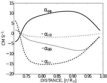
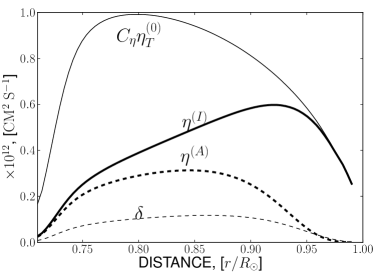
Figure 1: Left, the profiles of the $\alpha$ effects components for the $\theta=45^{\circ}$. Right, the profiles of the background turbulent diffusivity $C_{\eta}\eta_{T}$, the isotropic, $\eta^{(I)}$, and anisotropic, $\eta^{(A)}$, parts of the magnetic diffusivity and $\Omega\times J$ effect (also known as $\delta$ effect (Rädler 1969; Stix 1976).

The contribution of small-scale magnetic helicity $\overline{\chi}=\overline{\boldmath{a\cdot}\boldmath{b}}$ to the $\alpha$-effect is defined as

$$\alpha_{ij}^{(M)}=2f_{2}^{(a)}\delta_{ij}\frac{\overline{\chi}\tau_{c}}{\mu_{0}\overline{\rho}\ell^{2}}-2f_{1}^{(a)}e_{i}e_{j}\frac{\overline{\chi}\tau_{c}}{\mu_{0}\overline{\rho}\ell^{2}}.$$ (15)

The nonlinear feedback of the large-scale magnetic field to the $\alpha$-effect is described by a dynamical quenching due to the constraint of magnetic helicity conservation given by Eq.(8). For the illustration purpose we use the realistic value for the magnetic Reynolds number $R_{m}=10^{6}$. We matched the potential field outside and the perfect conductivity at the bottom boundary with the standard boundary conditions. For the magnetic helicity the number of the possibilities can be used (Guerrero et al. 2010; Mitra et al. 2010). We employ $\nabla_{r}\left(\bar{\chi}+\overline{\mathbf{A}}\cdot\overline{\mathbf{B}}\right)=0$ at the top of the domain and $\bar{\chi}=0$ at the bottom of the convection zone to show that for the $\alpha$-quenching formalism which is based on the Eq.(8), the boundary conditions determine the dynamics of the dynamo wave at the near surface layer. To evolve the Eq.(8) we have to define the large-scale vector potential for each time-step. For the axisymmetric large-scale magnetic fields where the vector-potential is

$$\overline{\mathbf{A}}=\mathbf{e}_{\phi}P+\mathbf{r}T=\frac{R^{2}\mathbf{e}_{\phi}}{r\sin\theta}A+r\mathbf{e}_{r}T.$$ (16)

The toroidal part of the vector potential is governed by the dynamo equations. The poloidal part of the vector potential can be restored from equation $\boldsymbol{\nabla}\times\left(\mathbf{r}T\right)=\mathbf{e}_{\phi}B$.

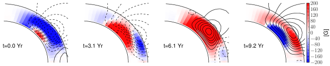
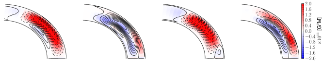
Figure 2: Snapshots of the magnetic field and helicity evolution inside the North segment of the convection zone. Top panel panel shows the field lines of the poloidal component of the mean magnetic field and the toroidal magnetic field (varies $\pm 700$G) by gray scale density plot. The bottom panel shows the large-scale (density plot) and small-scale magnetic helicity (contours) distributions.

Figure 2 shows the snapshots of the magnetic field and magnetic helicity (large- and small-scale) evolution in the North segment of the solar convection zone. The Figure shows the drift of the dynamo waves which are related to the large-scale toroidal and poloidal fields towards the equator and towards the pole, respectively. The distributions of the large- and small-scale magnetic helicities show one to one correspondence in sign. This is in agreement with Eq.(8). It is seen that the negative sign of the magnetic helicity follows to the dynamo wave of the toroidal magnetic field. This can be related to the so-called “current helicity hemisperic rule” which is suggested by the observations (Seehafer 1990; Zhang et al. 2010). The origin of the helicity rule has been extensively studied in the dynamo theory (Fisher et al. 1999; Choudhuri et al. 2004; Kuzanyan et al. 2006; Sokoloff et al. 2006; Pevtsov & Longcope 2007; Pipin & Kosovichev 2011b; Zhang et al. 2012).

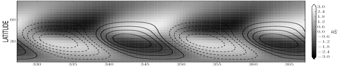
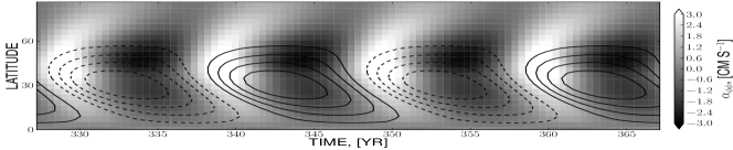
Figure 3: Top, the time - latitude variations of the toroidal field near the surface, $r=0.95R_{\odot}$, (contours $\pm 300$G) and the radial magnetic field at the surface (density plot). Bottom, the same for the the toroidal field and the $\alpha$ effect ($\alpha_{\phi\phi}$ component)(density plot).

The time-latitude diagrams for the dynamo model are shown in Figure 3. The results are in qualitative agreement with observations. We show the dynamical $\alpha$ effect as well. The model shows that with the given boundary conditions the $\alpha$ effect increases and has positive maximum at the growing phase of the cycle and it decreases, having the negative minimum at the decaying phase of the cycle. The variations of the radial profiles for the $\alpha$ effect and the small-scale-magnetic helicity are shown in Figure 4. The saddle in the the $\alpha$ effect profile is resulted from the given boundary conditions and distribution of the large-scale magnetic field near the top of the solar convection zone. The latter is determined by the dynamo boundary conditions and by the subsurface shear layer. It was found that the saddle disappears in case of $\nabla_{r}\bar{\chi}=0$ at the top. The highly non-uniform radial distribution of the $\alpha$ effect (at least for the near-equatorial latitudes) was found in the global LES (large-scale eddy) simulation of the dynamo action in the recent paper by Racine et al. (2011).

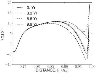
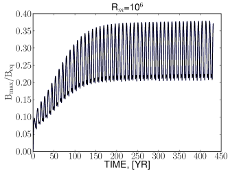
Figure 4: Left panel shows variations of the $\alpha$ effect ($\alpha_{\phi\phi}$ component) profiles with the cycle at colatitude $\theta=45^{\circ}$, the kinetic part of the $\alpha$ effect is shown by the solid line. Right panel shows the ratio of the maximum of the toroidal field strength and the equipartition value with time. .

The results obtained with the given dynamo model can be summarized as follows. In the model the dynamo wave propagates through the convection zone and shaped by the subsurface shear layer. The model incorporates the fairly complete expressions for the mean-electromotive force, including the anisotropic turbulent pumping and magnetic diffusivity, the turbulent generation of the poloidal and the toroidal fields due to $\alpha^{2}$ and $\Omega\times J$ effects and the dynamical $\alpha$ quenching due to magnetic helicity.We demonstrate that the conservation of the total helicity given in the form of Eq.(8) alleviates the catastrophic quenching (see Figure 4) for the solar type dynamos that operates on the base of the $\alpha\Omega$ mechanism. The further development can be related to the nonlocal framework for the mean-electromotive force.

6 Conclusions

Summarizing the main topics of this review, which I also consider as a principal advances in the mean-field dynamo theory, I conclude as follows. Firstly, the knowledge of the mean-field coefficients is decisive in order to analyze and model dynamo action in a variety astrophysical bodies. It was found that agreement between the direct numerical simulation and mean-field models is good only if a large number of mean-field coefficients are involved, which contribute to $\alpha$, $\gamma$, $\eta$, $\kappa$ (see, Eq.2). One obvious reason for this is that the spatial scale-separation is not valid for many astrophysical cases. Secondly, the issues related to the catastrophic quenching of the dynamo can be alleviated by different ways. However, the approach, which is based on conservation of the total helicity, see Eq.(8), suggests just a more than the way around the catastrophic quenching issue. It was proved that the magnetic helicity conservation does not pose an issue for the solar type dynamos. The new formalism can be used to study the origin of the different kind of anomalies in solar magnetic activity, which are observed and related to evolution of the large-scale toroidal field, the surface distribution of the magnetic helicity at different phase of the solar cycle etc. These points have not been discussed in this review and remain an open field for the future work.

Acknowledgments I thank for the support the RFBR grants 12-02-00170-a, 10-02-00148-a and 10-02-00960, the support of the Integration Project of SB RAS N 34, and support of the state contracts 02.740.11.0576, 16.518.11.7065 of the Ministry of Education and Science of Russian Federation.

References

- Blackman & Field (2002) Blackman, E. G., & Field, G. B. 2002, Physical Review Letters, 89, 265007
- Bonanno et al. (2002) Bonanno, A., Elstner, D., Rüdiger, G., & Belvedere, G. 2002, A&A, 390, 673
- Brandenburg (2001) Brandenburg, A. 2001, ApJ, 550, 824
- Brandenburg (2005) —. 2005, ApJ, 625, 539
- Brandenburg (2006) Brandenburg, A. 2006, in Astronomical Society of the Pacific Conference Series, Vol. 354, Solar MHD Theory and Observations: A High Spatial Resolution Perspective, ed. J. Leibacher, R. F. Stein, & H. Uitenbroek, 121–+
- Brandenburg & Käpylä (2007) Brandenburg, A., & Käpylä, P. J. 2007, New Journal of Physics, 9, 305
- Brandenburg et al. (2012) Brandenburg, A., Rädler, K.-H., & Kemel, K. 2012, A&A, 539, A35
- Brandenburg et al. (2008a) Brandenburg, A., Rädler, K.-H., Rheinhardt, M., & Käpylä, P. J. 2008a, ApJ, 676, 740
- Brandenburg et al. (2008b) Brandenburg, A., Rädler, K.-H., & Schrinner, M. 2008b, A&A, 482, 739
- Brandenburg & Sokoloff (2002) Brandenburg, A., & Sokoloff, D. 2002, Geophys. Astrophys. Fluid Dyn., 96, 319
- Brandenburg & Subramanian (2005) Brandenburg, A., & Subramanian, K. 2005, Phys. Rep., 417, 1
- Brown et al. (2011) Brown, B. P., Browning, M. K., Brun, A. S., Miesch, M. S., & Toomre, J. 2011, in Astronomical Society of the Pacific Conference Series, Vol. 448, 16th Cambridge Workshop on Cool Stars, Stellar Systems, and the Sun, ed. C. Johns-Krull, M. K. Browning, & A. A. West, 277
- Choudhuri et al. (2004) Choudhuri, A. R., Chatterjee, P., & Nandy, D. 2004, ApJ, 615, L57
- Dittrich et al. (1984) Dittrich, P., Molchanov, S. A., Sokolov, D. D., & Ruzmaikin, A. A. 1984, Astronomische Nachrichten, 305, 119
- Fisher et al. (1999) Fisher, G. H., Longcope, D. W., Linton, M. G., Fan, Y., & Pevtsov, A. A. 1999, in Astronomical Society of the Pacific Conference Series, Vol. 178, Stellar Dynamos: Nonlinearity and Chaotic Flows, ed. M. Nunez & A. Ferriz-Mas, 35
- Guerrero et al. (2010) Guerrero, G., Chatterjee, P., & Brandenburg, A. 2010, MNRAS, 409, 1619
- Guerrero & de Gouveia Dal Pino (2008) Guerrero, G., & de Gouveia Dal Pino, E. M. 2008, A&A, 485, 267
- Guerrero & de Gouveia Dal Pino (2009) Guerrero, G., & de Gouveia Dal Pino, E. M. 2009, in Revista Mexicana de Astronomia y Astrofisica Conference Series, Vol. 36, Revista Mexicana de Astronomia y Astrofisica Conference Series, 252
- Harvey (2000) Harvey, K. 2000, Solar Active Regions: Ephemeral, ed. P. Murdin
- Hubbard & Brandenburg (2012) Hubbard, A., & Brandenburg, A. 2012, ApJ, 748, 51
- Käpylä & Brandenburg (2007) Käpylä, P. J., & Brandenburg, A. 2007, Astronomische Nachrichten, 328, 1006
- Käpylä et al. (2008) Käpylä, P. J., Korpi, M. J., & Brandenburg, A. 2008, A&A, 491, 353
- Käpylä et al. (2009) —. 2009, A&A, 500, 633
- Kichatinov (2003) Kichatinov, L. L. 2003, R. Erdelyi et al(eds.), Turbulence, Waves and Instabilities in the Solar Plasma, Kluwer, 81
- Kichatinov et al. (1994) Kichatinov, L. L., Pipin, V., & Rüdiger, G. 1994, Astron. Nachr., 315, 157
- Kitchatinov (2002) Kitchatinov, L. L. 2002, A&A, 394, 1135
- Kitchatinov & Olemskoy (2011) Kitchatinov, L. L., & Olemskoy, S. V. 2011, Astronomy Letters, 37, 286
- Kleeorin et al. (1996) Kleeorin, N., Mond, M., & Rogachevskii, I. 1996, A&A, 307, 293
- Kleeorin et al. (2000) Kleeorin, N., Moss, D., Rogachevskii, I., & Sokoloff, D. 2000, A&A, 361, L5
- Kleeorin & Rogachevskii (1999) Kleeorin, N., & Rogachevskii, I. 1999, Phys. Rev.E, 59, 6724
- Kleeorin & Rogachevskii (2003) Kleeorin, N., & Rogachevskii, I. 2003, Phys. Rev. E, 67, 026321
- Krause & Rädler (1980) Krause, F., & Rädler, K.-H. 1980, Mean-Field Magnetohydrodynamics and Dynamo Theory (Berlin: Akademie-Verlag), 271
- Kuzanyan et al. (2006) Kuzanyan, K. M., Pipin, V. V., & Seehafer, N. 2006, Sol.Phys., 233, 185
- Livermore et al. (2010) Livermore, P. W., Hughes, D. W., & Tobias, S. M. 2010, Physics of Fluids, 22, 037101
- Makarov & Makarova (1996) Makarov, V. I., & Makarova, V. V. 1996, Sol. Phys., 163, 267
- Makarov et al. (2004) Makarov, V. I., Tlatov, A. G., & Callebaut, D. K. 2004, in IAU Symposium, Vol. 223, Multi-Wavelength Investigations of Solar Activity, ed. A. V. Stepanov, E. E. Benevolenskaya, & A. G. Kosovichev, 49–56
- Mitra et al. (2010) Mitra, D., Candelaresi, S., Chatterjee, P., Tavakol, R., & Brandenburg, A. 2010, Astronomische Nachrichten, 331, 130
- Mitra et al. (2011) Mitra, D., Moss, D., Tavakol, R., & Brandenburg, A. 2011, A&A, 526, A138+
- Moffatt (1978) Moffatt, H. K. 1978, Magnetic Field Generation in Electrically Conducting Fluids (Cambridge, England: Cambridge University Press)
- Monin & Yaglom (1975) Monin, A. S., & Yaglom, A. M. 1975, Statistical fluid mechanics: Mechanics of turbulence. Volume 2 /revised and enlarged edition/ (MIT)
- Morin et al. (2011) Morin, J., Dormy, E., Schrinner, M., & Donati, J.-F. 2011, MNRAS, 418, L133
- Ossendrijver et al. (2001) Ossendrijver, M., Stix, M., & Brandenburg, A. 2001, A&A, 376, 713
- Ossendrijver et al. (2002) Ossendrijver, M., Stix, M., Brandenburg, A., & Rüdiger, G. 2002, A&A, 394, 735
- Parker (1955) Parker, E. 1955, Astrophys. J., 122, 293
- Parker (1979) Parker, E. N. 1979, Cosmical magnetic fields: Their origin and their activity (Oxford: Clarendon Press)
- Parnell et al. (2009) Parnell, C. E., DeForest, C. E., Hagenaar, H. J., Johnston, B. A., Lamb, D. A., & Welsch, B. T. 2009, ApJ, 698, 75
- Pevtsov & Longcope (2007) Pevtsov, A. A., & Longcope, D. W. 2007, in Astronomical Society of the Pacific Conference Series, Vol. 369, New Solar Physics with Solar-B Mission, ed. K. Shibata, S. Nagata, & T. Sakurai, 99
- Pipin (2008) Pipin, V. V. 2008, Geophysical and Astrophysical Fluid Dynamics, 102, 21
- Pipin & Kosovichev (2011a) Pipin, V. V., & Kosovichev, A. G. 2011a, ApJ, 738, 104
- Pipin & Kosovichev (2011b) —. 2011b, ApJ, 741, 1
- Pipin & Kosovichev (2011c) —. 2011c, ApJL, 727, L45
- Pipin & Seehafer (2009) Pipin, V. V., & Seehafer, N. 2009, A&A, 493, 819
- Pipin & Sokoloff (2011) Pipin, V. V., & Sokoloff, D. D. 2011, Physica Scripta, 84, 065903
- Pouquet et al. (1975) Pouquet, A., Frisch, U., & Léorat, J. 1975, J. Fluid Mech., 68, 769
- Racine et al. (2011) Racine, É., Charbonneau, P., Ghizaru, M., Bouchat, A., & Smolarkiewicz, P. K. 2011, ApJ, 735, 46
- Rädler et al. (2003) Rädler, K., Kleeorin, N., & Rogachevskii, I. 2003, Geophysical and Astrophysical Fluid Dynamics, 97, 249
- Rädler (1969) Rädler, K.-H. 1969, Monats. Dt. Akad. Wiss., 11, 194
- Rädler et al. (2003) Rädler, K.-H., Kleeorin, N., & Rogachevskii, I. 2003, Geophys. Astrophys. Fluid Dyn., 97, 249
- Rädler & Rheinhardt (2007) Rädler, K.-H., & Rheinhardt, M. 2007, Geophysical and Astrophysical Fluid Dynamics, 101, 117
- Rempel (2006) Rempel, M. 2006, ApJ, 647, 662
- Rheinhardt & Brandenburg (2010) Rheinhardt, M., & Brandenburg, A. 2010, A&A, 520, A28
- Rheinhardt & Brandenburg (2012) —. 2012, Astronomische Nachrichten, 333, 71
- Rogachevskii & Kleeorin (2003) Rogachevskii, I., & Kleeorin, N. 2003, Phys. Rev.E, 68, 1
- Rogachevskii et al. (2011) Rogachevskii, I., Kleeorin, N., Käpylä, P. J., & Brandenburg, A. 2011, Phys. Rev. E, 84, 056314
- Rüdiger & Hollerbach (2004) Rüdiger, G., & Hollerbach, R. 2004, The Magnetic Universe (Wiley-Vch Verlag)
- Rüdiger & Kitchatinov (2000) Rüdiger, G., & Kitchatinov, L. L. 2000, Astronomische Nachrichten, 321, 75
- Ruediger & Brandenburg (1995) Ruediger, G., & Brandenburg, A. 1995, A&A, 296, 557
- Schrinner (2011) Schrinner, M. 2011, A&A, 533, A108
- Schrinner et al. (2012) Schrinner, M., Petitdemange, L., & Dormy, E. 2012, ApJ, 752, 121
- Schrinner et al. (2005) Schrinner, M., Rädler, K.-H., Schmitt, D., Rheinhardt, M., & Christensen, U. 2005, Astronomische Nachrichten, 326, 245
- Seehafer (1990) Seehafer, N. 1990, Sol. Phys., 125, 219
- Sokoloff et al. (2006) Sokoloff, D., Bao, S. D., Kleeorin, N., Kuzanyan, K., Moss, D., Rogachevskii, I., Tomin, D., & Zhang, H. 2006, Astron. Nachr., 327, 876
- Stenflo & Kosovichev (2012) Stenflo, J. O., & Kosovichev, A. G. 2012, ApJ, 745, 129
- Stix (1976) Stix, M. 1976, Astron. Astrophys., 47, 243
- Stix (2002) Stix, M. 2002, The sun: an introduction, 2nd edn. (Berlin : Springer), 521
- Subramanian & Brandenburg (2004) Subramanian, K., & Brandenburg, A. 2004, Phys. Rev. Lett., 93, 205001
- Tobias et al. (2011) Tobias, S. M., Dagon, K., & Marston, J. B. 2011, ApJ, 727, 127
- Vishniac & Cho (2001) Vishniac, E. T., & Cho, J. 2001, Astrophys. J., 550, 752
- Zel’dovich et al. (1984) Zel’dovich, Y. B., Ruzmaikin, A. A., Molchanov, S. A., & Sokolov, D. D. 1984, Journal of Fluid Mechanics, 144, 1
- Zhang et al. (2012) Zhang, H., Moss, D., Kleeorin, N., Kuzanyan, K., Rogachevskii, I., Sokoloff, D., Gao, Y., & Xu, H. 2012, ApJ, 751, 47
- Zhang et al. (2010) Zhang, H., Sakurai, T., Pevtsov, A., Gao, Y., Xu, H., Sokoloff, D. D., & Kuzanyan, K. 2010, MNRAS, 402, L30