Resonances for activity waves in spherical mean field dynamos

Abstract

We study activity waves of the kind that determine cyclic magnetic activity of various stars, including the Sun, as a more general physical rather than a purely astronomical problem. We try to identify resonances which are expected to occur when a mean-field dynamo excites waves of quasi-stationary magnetic field in two distinct spherical layers. We isolate some features that can be associated with resonances in the profiles of energy or frequency plotted versus a dynamo governing parameter. Rather unexpectedly however the resonances in spherical dynamos take a much less spectacular form than resonances in many more familiar branches of physics. In particular, we find that the magnitudes of resonant phenomena are much smaller than seem detectable by astronomical observations, and plausibly any related effects in laboratory dynamo experiments (which of course are not in gravitating spheres!) are also small. We discuss specific features relevant to resonant phenomena in spherical dynamos, and find parametric resonance to be the most pronounced type of resonance phenomena. Resonance conditions for these dynamo wave resonances are rather different from those for more conventional branches of physics. We suggest that the relative insignificance of the phenomenon in this case is because the phenomena of excitation and propagation of the activity waves are not well-separated from each other and this, together with the nonlinear nature of more-or-less realistic dynamos, suppress the resonances and makes them much less pronounced than resonant effects, for example in optics,.

I Introduction

The well known solar activity cycle is associated with propagation of a wave of quasistationary magnetic field somewhere within the solar convective envelope. This wave is believed to be excited and supported by electromagnetic induction effects driven by the joint action of differential rotation and mirror-asymmetric flows. This is known as dynamo action, e.g. S04 . Correspondingly, the wave is known as a dynamo wave. More specifically, there are at least two, more or less independent, dynamo waves, one propagating equatorwards in each solar hemisphere.

For quite a long time, solar activity waves provided the unique example of dynamo wave propagation, and so the phenomenon was not investigated in a wider context. Even such a limited statement of the problem provides a quite rich range of instructive physical phenomena. From time to time the dynamo engine ”misfires”, and solar Grand Minima, including the Maunder Minimum in the XVIIth - early XVIIIth centuries, occur (see for review e.g. SY03 ). At the end of the Maunder Minimum, the dynamo wave propagated in one solar hemisphere only, and a so-called ”mixed-parity” magnetic configuration appeared SNR94 . Analysis of XVIIIth century sunspot data A08 gives a hint Ietal10 that from time to time magnetic field becomes concentrated near to the solar equator, rather than in two propagating belts in middle latitudes, and a configuration of quadrupole-like (instead of the usual dipole-like) symmetry then appears.

Recently the variety of physical phenomenon associated with dynamo wave propagation has enlarged substantially. The first attempts to isolate dynamo wave propagation from stellar activity data were undertaken in BH07 ; K10 , and generation of oscillating magnetic field, probably indicating dynamo wave propagation, was obtained in the VKS dynamo experiment Metal07 . This opens new perspectives in the topic, in particular the opportunity to study dynamo waves as a physical, rather than a purely astronomical, phenomenon.

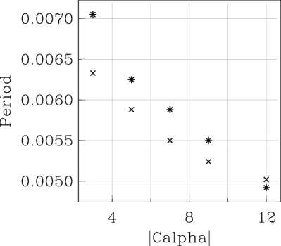
Figure 1: Periods of oscillation in energy when dynamo action occurs in a single layer. Crosses: $C^{I}_{\alpha}=0$, $C^{II}_{\alpha}$ varies; asterisks: $C^{II}_{\alpha}=0$, $C^{I}_{\alpha}$ varies .

This change of viewpoint in the investigation of dynamo waves has attracted attention to these problems, which had previously remained underinvestigated. In particular, it was stressed DG12 that resonance, which is a prominent and sometimes spectacular phenomenon in the conventional theory of various oscillations and wave propagations, must also play an important role in dynamo wave propagation. We share their view that the topic was not adequately addressed in previous studies, and only a few papers (including KS93 ; Moss96 ) have addressed the topic. The point is that the natural statement of the problem relevant to astronomical contexts did not focus attention on this issue.

Here we present our findings associated with the problem of resonance phenomena in dynamo wave propagation. Our general conclusion can be formulated as follows. Resonances in dynamo systems do occur, and sometimes they can be isolated in the solutions of the governing equations (e.g. KS93 ; Moss96 ). However in general dynamo wave propagation as a physical phenomenon differs quite substantially from, say, the propagation of acoustic or electromagnetic waves. The point is that conventional wave propagation can be easily separated from the wave excitation, whereas dynamo wave propagation is usually intimately associated with dynamo wave excitation. As a result, solutions of the dynamo equations usually fail to separate in any explicit way resonant phenomena from the more general phenomena of dynamo wave excitation.

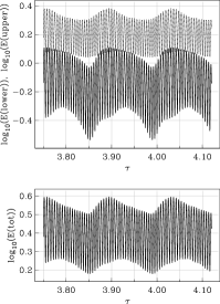
Figure 2: Time variations of magnetic energy for $C_{\alpha}^{I}=6,C_{\alpha}^{II}=-5$. Upper panel - toroidal field energy in lower (solid curve) and upper (broken) layers separately, lower panel - total magnetic energy.

We illustrate the problem by numerical investigation of a dynamo model in which dynamo waves are excited in two adjacent spherical shells with different distributions of dynamo governing parameters. The magnetic field is continuous across the boundary between the two domains. A related model was discussed previously in MS07 ; MSL11 in a more specifically astronomical context.

II The dynamo model

We consider a standard mean field dynamo equation ($\alpha^{2}\omega$-dynamo)

$${\frac{\partial{\bf B}}{\partial t}}={\rm curl}\,({\bf V\times B}+\alpha{\bf B}-\eta\,{\rm curl}\,{\bf B}),$$ (1)

where $\eta$ is the turbulent diffusivity and $\alpha$ represents the usual isotropic alpha-effect (for details of the model see MS07 ; the codes used there are in turn based on that of MB00 ). In Eq. (1) $\bf V$ is the velocity from the (differential) rotation and we only look for axisymmetric solutions. A simple algebraic $\alpha$-quenching (in which $\alpha$ is reduced by a factor $1+(B/B_{0})^{2}$, where $B_{0}$ is a field strength at which dynamo saturation is expected) is used to suppress dynamo action as the magnetic field grows.

Figure 3: The case $C_{\alpha}^{II}=-5$, $C_{\omega}^{I}=C_{\omega}^{II}=10^{5}$. Top panel: toroidal field energies in the lower and upper layers (asterisks and crosses respectively). The lower panel shows the total energy and the middle panel shows the variation of the period of oscillation of the energy. In each panel, quantities are plotted as a function of $C_{\alpha}^{I}$.

We solve the equation in spherical geometry for two adjacent dynamo active layers, the ’deep’ layer I with $0.7\leq r\leq 0.85$ and the ’shallow’ layer II with $0.85\leq r\leq 1$ ($r$ is the fractional radius). We consider a very simple rotation profile with rotation velocity linear in $r$, and $\alpha$-profiles in each layer are proportional to $\cos\theta$ where $\theta$ is the polar angle, so that $\theta=90^{\circ}$ is the equator. $C^{I}_{\alpha}$ and $C^{II}_{\alpha}$ are dimensionless amplitudes of $\alpha$ in layers I and II correspondingly, and $C^{I}_{\omega}$ and $C^{II}_{\omega}$ are dimensionless amplitudes of the differential rotation. We take $C^{I}_{\omega}=C^{II}_{\omega}$ in the examples discussed below. $\alpha$ is continuous across the interface at $r=0.85$. All solutions discussed have odd (”dipole-like”) parity.

Our investigation is focussed on the more physical aspects of the problem, but it would be straightforward to rescale the results for particular celestial bodies, or to take a more realistic rotation curve.

III Looking for resonance in dynamo solutions

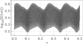
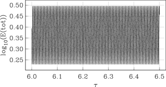
Figure 4: Extracts from the time series of total energy for solutions outside of the resonant domain (upper panel, $C^{I}_{\alpha}=6.5$), and inside this domain (lower panel, $C^{I}_{\alpha}=4.5$).

III.1 Background

We obtained solutions for our model for various governing parameters. We first determined the periods when dynamo action occurs in one layer only, i.e. either $C_{\alpha}^{I}$ or $C_{\alpha}^{II}$ is zero. Note that the magnetic field does penetrate the passive layer, although its strength is substantially reduced there. Here we either take $C_{\alpha}^{I}>0$ so that with $C_{\alpha}^{II}=0$ we obtain poleward migration, or $C_{\alpha}^{II}<0$ so that with $C_{\alpha}^{I}=0$ there is equatorward migration. The variations of period with $|C_{\alpha}^{I,II}|$ for these cases are shown in Fig. 1.

More generally, the model includes two interacting dynamo regions, which are physically separate but adjacent, which possess specific individual eigenfrequencies, so quite naturally the resulting time-series for the total magnetic energy and magnetic energy for the upper and lower layer can be more complicated than just a harmonic oscillation; see Fig. 2 where the result for a typical solution ($C_{\alpha}^{I}=6,C_{\alpha}^{II}=-5$) is shown.

III.2 Resonant solutions

We then set $C_{\alpha}^{II}=-5$ and allowed $C_{\alpha}^{I}$ to vary, and plotted the period of the total energy (defined by a mean over $O(1000)$ oscillations) The variations of toroidal field energies in the upper and lower layers, the (common) period and the total magnetic energy are shown in Fig. 3 as a function of $C_{\alpha}^{I}$. We see a feature, in the form of a local peak of period, in the region $C^{I}_{\alpha}=5\pm 1$. A related feature appears in the plots of all three quantities (although it is maybe less pronounced in the lower panel). Examination of Fig. 2 shows that this feature does not correspond to $C_{\alpha}^{I}$ values for which the periods of the layers, taken individually, are equal. For $C_{\alpha}^{II}=-5$, periods are approximately equal when $C_{\alpha}^{I}\approx 7$.

We show in Fig. 4 short samples of the time series of the total energy for solutions outside of the resonant domain ($C_{\alpha}^{I}=6.5$, upper panel), and inside the domaon ($C_{\alpha}^{I}=4.5$, lower panel).

III.3 Resonance with a subcritical dynamo layer

Figure 5: The case $C_{\alpha}^{I}=-5$, $C_{\omega}^{I}=C_{\omega}^{II}=10^{5}$, with thin lower layer, $0.7\leq r\leq 0.775$. Top panel: toroidal field energies in the lower and upper layers (asterisks and crosses respectively). The lower panel shows the total energy and the middle panel shows the variation of period.

We recognize that the resonant behaviour was not very well pronounced in the previous results and thus try to explore and explain this situation. We do not doubt that resonance in its purely mathematical sense occurs in dynamo solutions. More specifically, if the governing equations for a kinematic dynamo problem have a degenerate eigenvalue $\Gamma_{n}=\gamma_{n}+i\omega_{n}$ ($\gamma_{n}>0$), then it is more than plausible that the corresponding set of eigenvectors becomes insufficient to provide a basis, and the desired solution, apart from terms proportional to $\exp(\gamma_{n}+i\omega_{n})t$, may contain resonant terms proportional to $t\exp(\gamma_{n}+i\omega_{n})t$. The point however is that the exponential growth of the solution as $\exp\gamma_{n}t$ or $t\exp\gamma_{n}t$ occurs just at the initial stage of the dynamo wave excitation and is a matter of more or less purely theoretical interest. A more practical issue is the amplitude of the steady-state oscillation obtained after the exponential growth is somehow saturated – here by the term $1+(B/B_{0})^{2}$. The saturation reduces the growth rate $\gamma_{n}$ to zero, and this is a much stronger effect than the additional power-low growth due to the resonance. The exceptional situation discussed by, say, KS93 ; Moss96 ) addresses the cases where excitation of a particular solution without a resonance does not occur, and it is the existence of a resonance that allows this solution to develop. In contrast, resonances in acoustic or electromagnetic wave propagation occur when a wave can marginally propagate and does not grow ($\gamma=0$), and the resonance is clearly recognisable as a growing (and then saturated) solution.

In another investigation, the lower layer was made much thinner $(0.7\leq r\leq 0.775)$, so a dynamo in this layer alone is subcritical (i.e. with $C_{\alpha}^{I}=\;\raise 1.29167pt\hbox{$<$\kern-7.5pt\raise-4.73611pt\hbox{$\sim$ }}\;\hskip-2.0pt10,C_{\alpha}^{II}=0$, dynamo action does not occur) and the upper layer correspondingly thicker, $0.775\leq r\leq 1.0$. We keep $C_{\alpha}^{II}=-5$, $C_{\omega}^{I}=C_{\omega}^{II}=10^{5}$. There is again a (smaller) feature attributable to a resonance near $C_{\alpha}^{I}=4.25$. See Fig. 5.

We conclude from Fig. 5 that the resonance here is of a similar nature to that in the previous case.

III.4 Parametric resonance

Now we seek the other kind of resonance, i.e. a parametric resonance in the dynamo wave driven by harmonic variations of the dynamo governing parameters. Our preliminary expectations here are twofold. From one hand, the resonances recognized in KS93 ; Moss96 for galactic dynamos are parametric. On the other hand, the parametric resonance suggested in MPS02 to explain some details in the magnetic activity of stellar binary systems does not seem very spectacular.

We imposed a modulation $\alpha=\alpha_{0}(1+f\cos\omega_{P}t)$ in the region I, with $500\leq\omega_{P}\leq 1500$, $f=0.2$, keeping $C_{\alpha}^{II}=-5$. We started from the unperturbed model which has $C_{\alpha}^{I}=7.5$ (i.e. outside of the resonant region discussed in Sect. III.2). The corresponding period is $P(E)=0.00539$, so $\omega(E)=1166$. Results are shown in Fig. 6, where resonant peaks are clearly recognizable.

The feature at $\omega_{P}\approx 1150$ is quite expected, as it satisfies the standard resonance condition $\omega_{P}\approx\omega(E)=2\omega(B)$ (where $\omega(B)$ is the frequency of the magnetic field oscillations). The features near $\omega_{p}\approx 700$ and $\omega_{p}\approx 900$ have to be associated with rather unusual excitation conditions. Note that these resonant solutions do not settle to a completely steady (maybe modulated) oscillation, even when run for about 2000 oscillations. In the two anomalous cases the period is not quite stable, but the averaging process seems robust, in that averages over different temporal sub-ranges give the same values. Note that the energy in the upper and lower regions separately (top panel in Fig. 6) is the toroidal field energy only, whereas the ”total energy” includes also the poloidal. Over long enough time intervals the average period in region II is slightly longer than that of the total energy (see middle panel of Fig. 6).

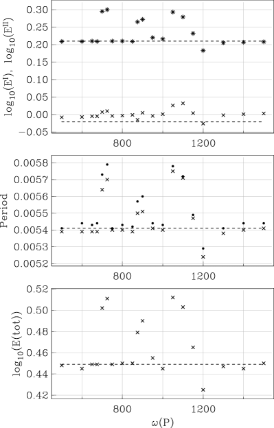
Figure 6: Parametric resonance: notation as in Fig. 3. The middle panel now includes the periods of oscillations in the upper layer II (shown by small solid circles). The dashed horizontal lines are values for the unperturbed model. The period of the total energy is plotted by solid dots in the middle panel. In each panel, quantities are plotted a functions of $\omega({\rm P})$.

In general, parametric resonance effects seem to be much clearer and more pronounced than the resonances analysed in previous models (Sects. III.2 and III.3). However the peaks in energy profiles for parametric resonances are quite broad.

IV Discussion

The concept of resonance belongs to the basic concepts of contemporary physics, and it looks a priori implausible that it should not be applicable to dynamo wave propagation. We have verified this natural expectation in the framework of activity waves generated by dynamo waves, in a quite traditional model of a two-layer mean-field spherical mean-field dynamo of the type conventionally considered as a model for periodic stellar magnetic activity.

Indeed, we found features in the profiles for energies or periods (frequencies) plotted versus a dynamo governing parameter which can be identified with a resonance. However, it looks noteworthy that the details resemble more discontinuities in the profiles of the behaviour of period and energy as $C_{\alpha}^{I}$ varies, rather than the conventional resonant peaks shown in physics textbooks. It is even difficult to claim that the resonance makes dynamo excitation more efficient and enhances, say, the total magnetic energy. The lower panel in Fig. 5 is instructive in this respect: the interaction here appears as a fall in total energy, rather than an increase. Of course, resonances are far from being the only effects that determine the relevant behaviour in, say, optics, and there are many cases where other effects make recognition of resonance peaks problematic. The point however is that it is not difficult to provide examples of pronounced resonant peaks in optics. When presenting our results, we have of course chosen the more pronounced examples of resonances for dynamo waves, admittedly from a rather small sample.

Correspondingly, we cannot suggest that the sort of resonances discussed here will leave observable signatures. Our intention is to draw attention to novel behaviour. Our results are not so marked as those in DG12 , arguably because a linear problem was considered there. The inclusion of a nonlinear saturation mechanism reduces these effects.

The parametric resonances present in the spherical dynamo models investigated here (Sect. III.4) are much clearer than the other resonance features (Sects. III.2 and III.3). Perhaps, this is a consequence of controlling by varying the frequency $\omega_{P}$, which governs the parametric excitation but, leaves unchanged the ”nominal” parameters of the dynamo model for the vanishing modulation amplitude $f=0$.

Our numerical experiment illuminate the unusual excitation conditions for parametric resonances. Perhaps, it can be said that the Mathieu equation is not a fully adequate model for parametric resonance in spherical dynamos. Isolation of the resonance condition here appears an attractive topic for dynamo theory, but it is however obviously beyond the scope of this paper. The transition time required for the dynamo system to achieve a resonant type solution can be long and a qualitative explanation in terms of an appropriate model equation also looks desirable.

We note also the existence of a quasi-resonant phenomenon in a case where one of the dynamo layers is passive, i.e. with the chosen parameters the lower layer taken in solution does not support dynamo action.

Perhaps the basic differences between resonant phenomena for dynamo waves and those in more conventional branches of physics can be summarized as follows. It is difficult to separate dynamo wave propagation from dynamo wave excitation, while such processes are well separated in many other branches of physics. Correspondingly, eigenvalues of the linear (kinematic) dynamo problems take complex values. Coincidence of two complex quantities is a more severe requirement rather than equality of two real valued quantities. Dynamo self-excitation is in practice saturated by some back-reaction of the dynamo generated magnetic field on the hydrodynamics. This saturation determines the resulting magnetic energy and affects the periods of dynamo waves. The corresponding effects specific to dynamo action are more important than any potential resonant behaviour. In additional, the two layers of dynamo action are separated hydrodynamically but magnetic field penetrates from one activity layer to the other, even if the dynamo action in one layer remains subcritical. Thus the very concept of the frequency of dynamo waves in one activity layer taken alone is not fully applicable.

In general, it seems that the situation under discussion reflects the every-day wisdom that small problems (here resonances) can only spoil your life in the absence of larger ones (in this case other uncertainties associated with mean field dynamos are much larger).

- (1) Stix, M., 2004, The Sun: An Introduction, B., Springer
- (2) Soon, W.W.-H., Yaskell, S.H., 2003, The Maunder Minimum: The Variable Sun-Earth Connection, Singapore, World Sci.
- (3) Sokoloff, D., Nesme-Ribes, E., 1994, Astron. Astrophys., 288, 293
- (4) Arlt, R., 2008, Solar Phys., 247, 399
- (5) Illarionov, E., Sokoloff, D., Arlt, R., Khlystova, A., 2011, Astronomische Nachrichten, 332, 590
- (6) Berdyugina, S.V., Henry, G.W., 2007, Astrophys. J., 659, L157
- (7) Katsova, M.M., Livshits, M.A., Soon, W., Baliunas, S.L., Sokoloff, D.D., 2010, New Astron., 15, 274
- (8) Monchaux, R., Berhanu, M., Bourgoin, M., Moulin, M., Odier, Ph., Pinton, J.-F., Volk, R., Fauve, S., Mordant, N., Petrelis, F., Chiffaudel, A., Daviaud, F., Dubrulle, B., Gasquet, C., Marié, L., Ravelet, F., 2007, PRL, 98, 044502
- (9) Gilman, P.A., Dikpati, M., 2011, Astrophys. J., 738, 108
- (10) Kuzanyan, K.M., Sokoloff, D.D., 1993, Astrophys. Sp. Sci., 208, 245
- (11) Moss, D., 1996, Astron. Astrophys., 308, 381
- (12) Moss, D., Sokoloff, D., 2007, Mon. Not. Roy. Astron. Soc., 377, 1597
- (13) Moss, D., Sokoloff, D.. Lanza, A. F., 2011, Astron. Astrophys., 531, A43
- (14) Moss, D., Brooke, J., 2000, Mon. Not. Roy. Astron. Soc., 315, 521
- (15) Moss, D., Piskunov, N., Sokoloff, D., 2002. Astron. Astrophys., 396, 885